

Estimation of Fractal Dimensions and Classification of Plant Disease with Complex Backgrounds

 , , , ,
  ,
,
Abstract
1. Introduction
- -
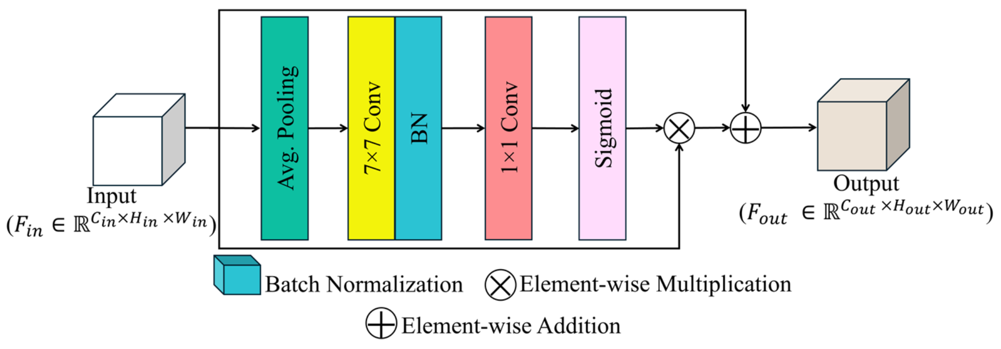
- We propose a residual convolution attention (RCA) block that enhances feature maps by focusing on disease-affected leaf regions, while suppressing irrelevant background noise. It applies attention weights to emphasize important disease-related features and uses residual connections to retain the original information.
- -
- Complex backgrounds in plant leaf disease images increase inter-class similarities and amplify intra-class differences. To address this issue, a residual concatenated block (RCB) is proposed to use parallel convolution to capture fine and coarse features, thereby increasing the inter-class differences. Additionally, batch normalization within the RCB module can help normalize the feature distributions by minimizing the internal covariant shift and reducing the variation within the same class. This module combines original input features and trained ones with a residual connection containing crucial information regarding the disease region.
- -
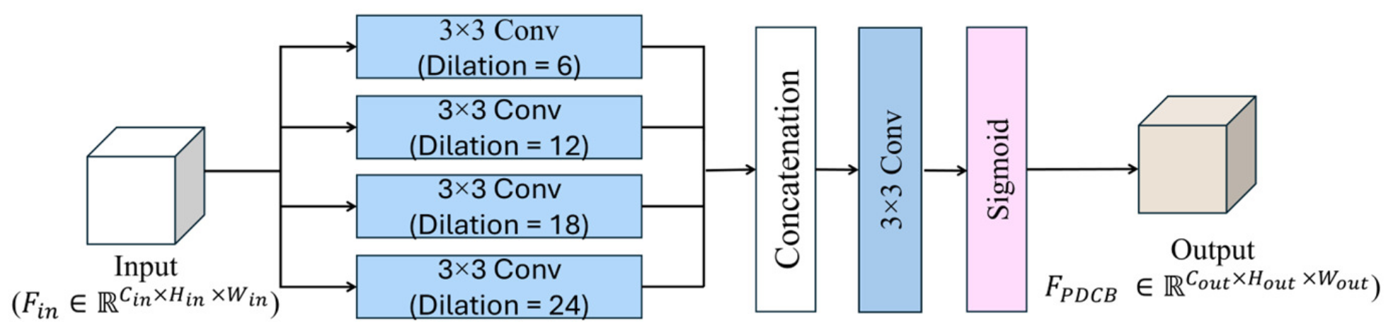
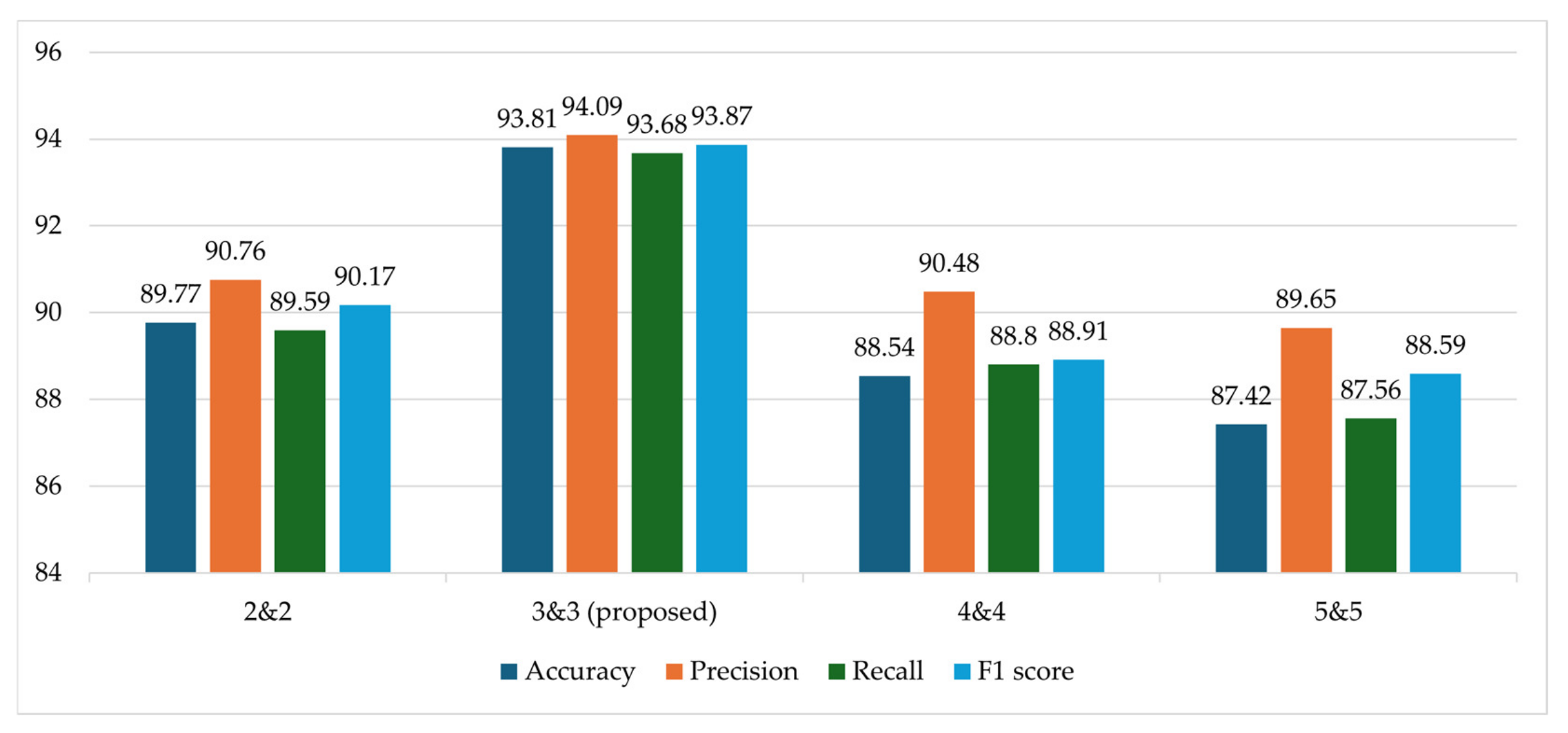
- The analyzed dataset contained various interfering elements in the background, such as leaves, branches, or soil. Therefore, a parallel dilated convolution block (PDCB) with four parallel convolutional layers, each with different dilation rates, is proposed to expand the receptive field without increasing the kernel size, acquiring features at multiple scales. This enables each layer to capture a wider context from the image, which is useful for identifying leaf patterns in infected areas from a complex background.
- -
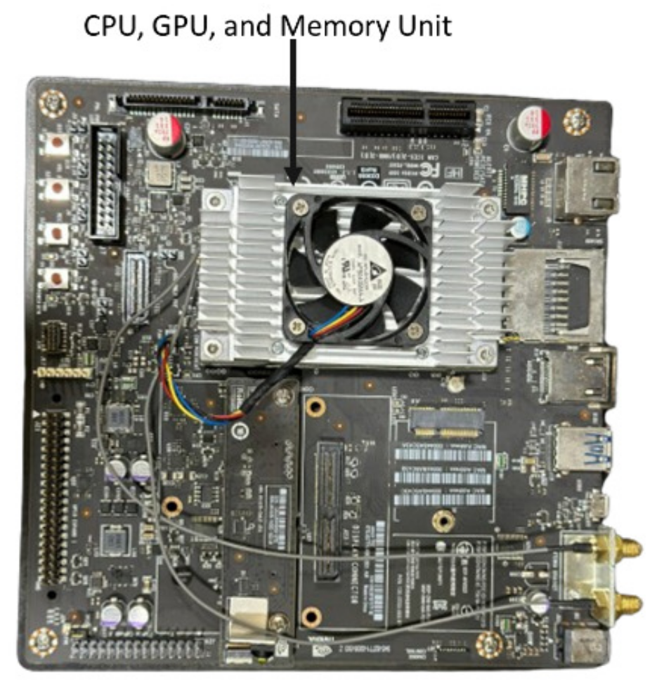
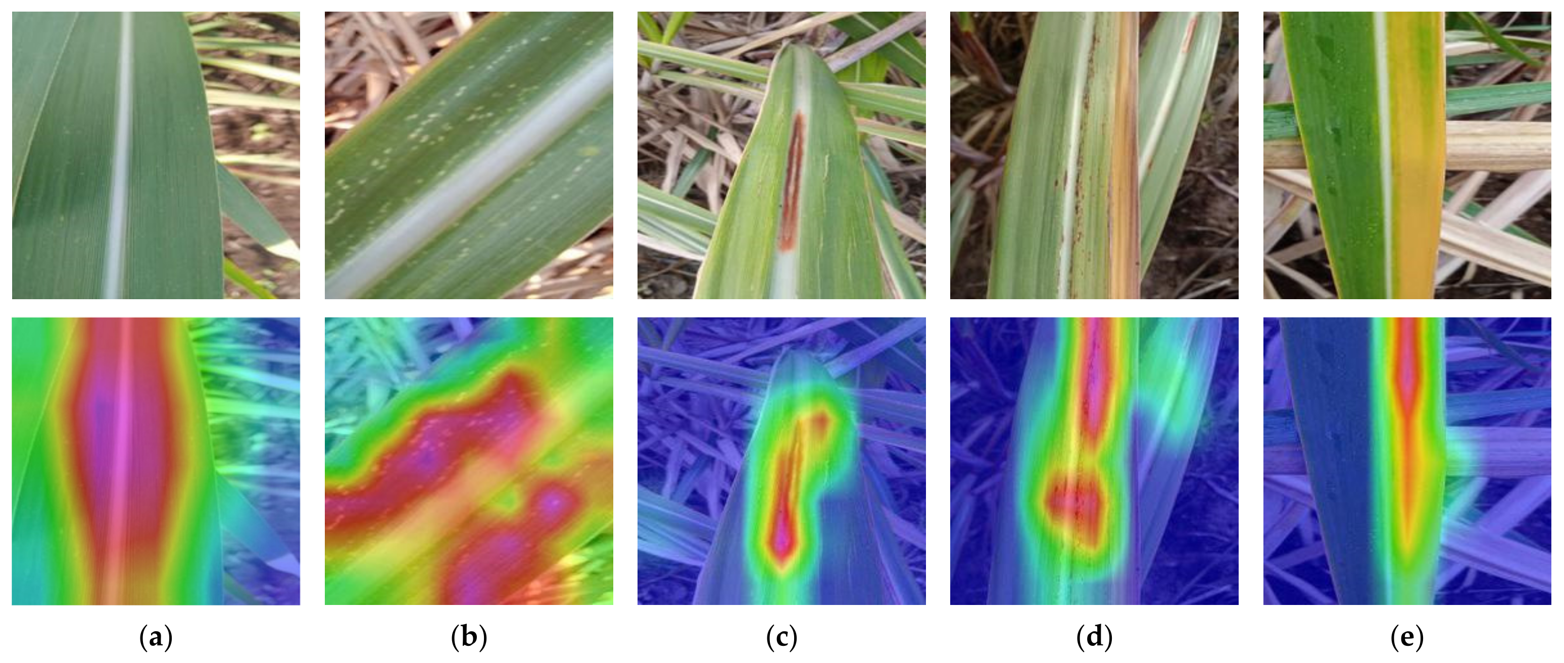
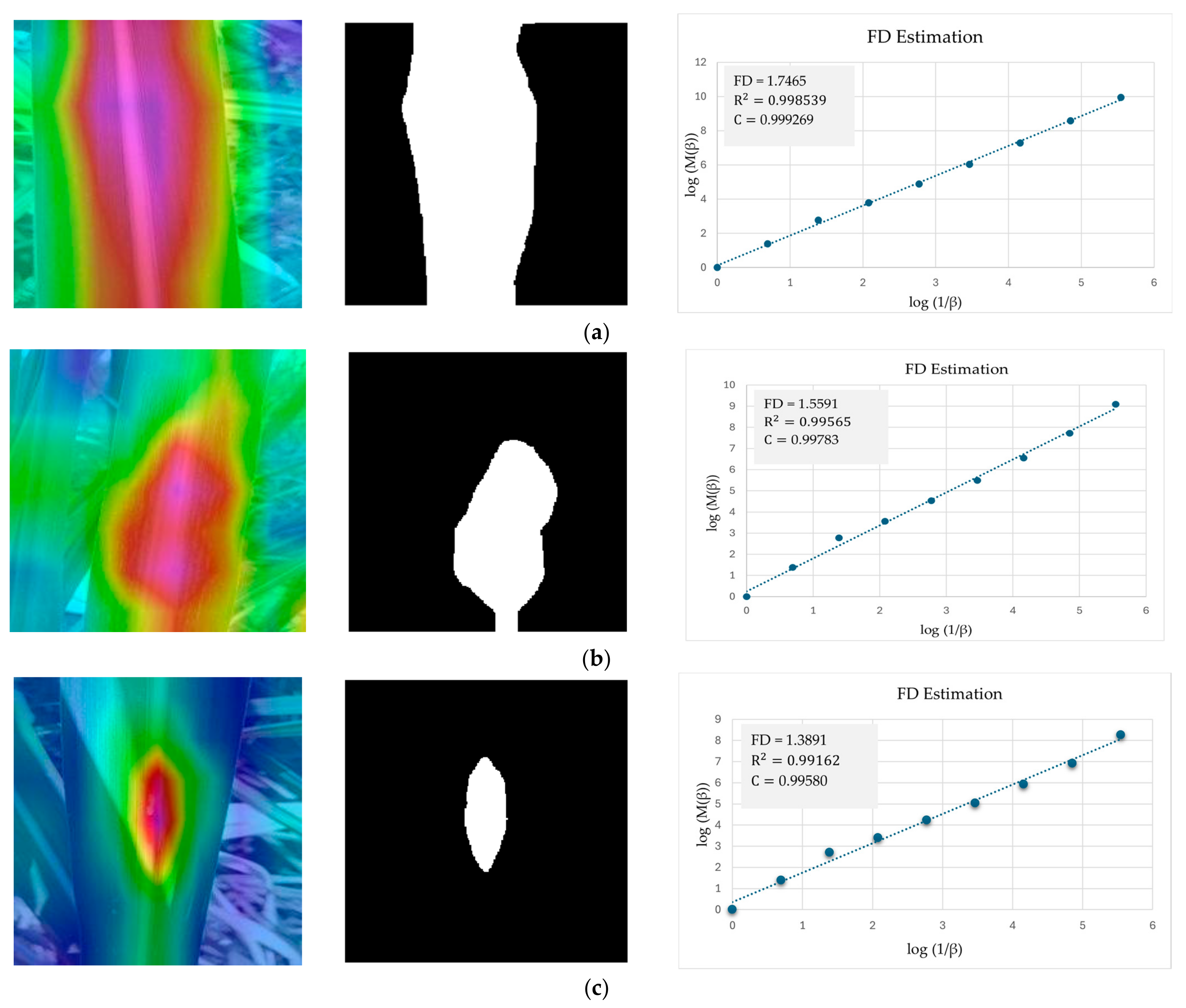
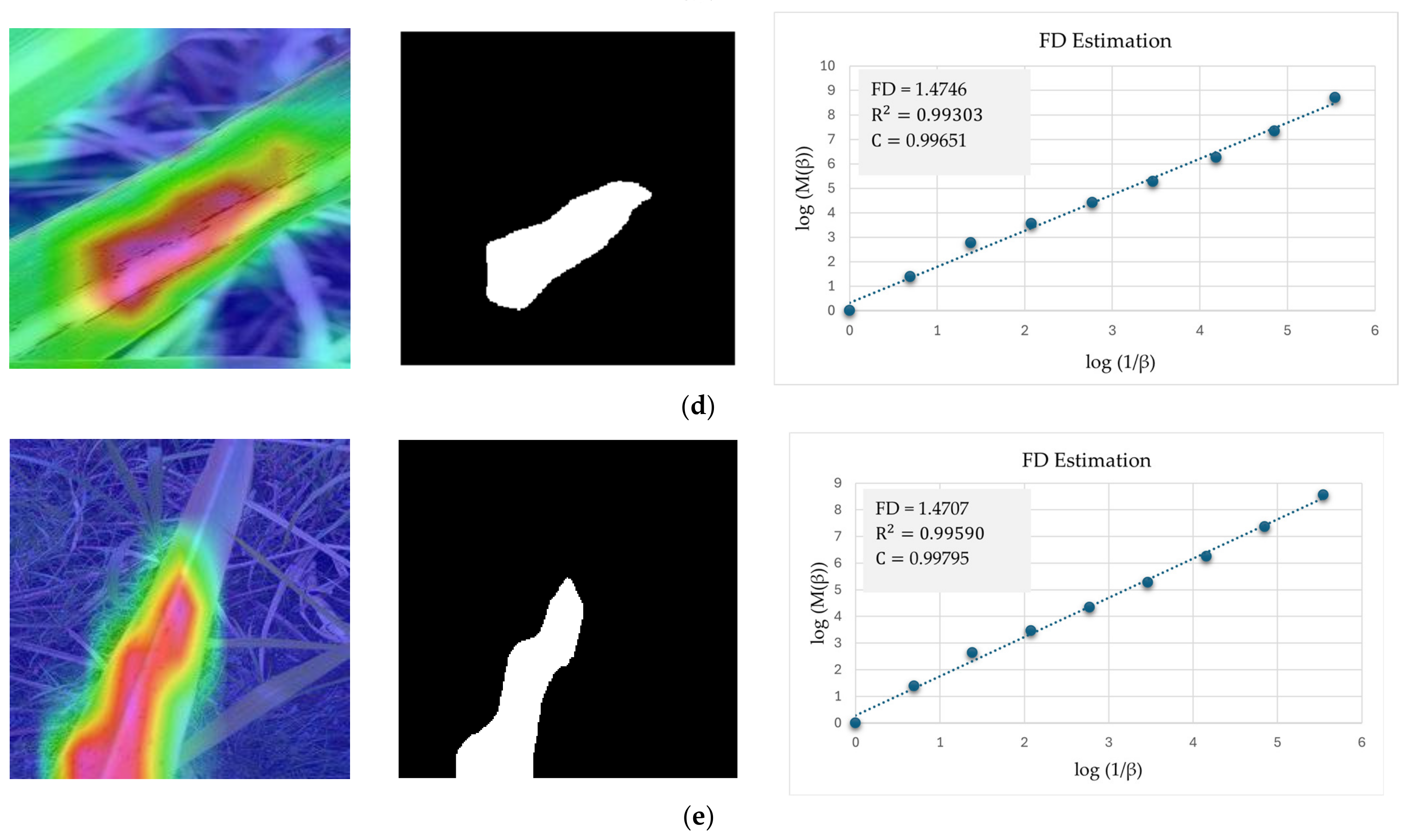
- We introduce the fractal dimension estimation to analyze the complexity and irregularity of class activation maps from the cases of healthy plants and their disease classes, confirming that our model can extract important features for the correct classification of plant disease. In addition, we confirm that our method can be operated on an embedded system for farming robots or mobile devices at fast processing speed (78.7 frames per second). Furthermore, our model and code are made publicly available on GitHub [10] for a fair comparison.
2. Related Work
2.1. Disease Classification of Images with Simple Background
2.1.1. ML-Based Methods
2.1.2. DL-Based Methods
2.2. Disease Classification of Images with Complex Background
3. Proposed Method
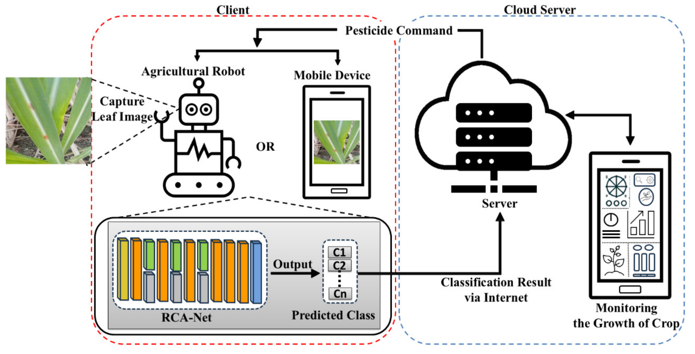
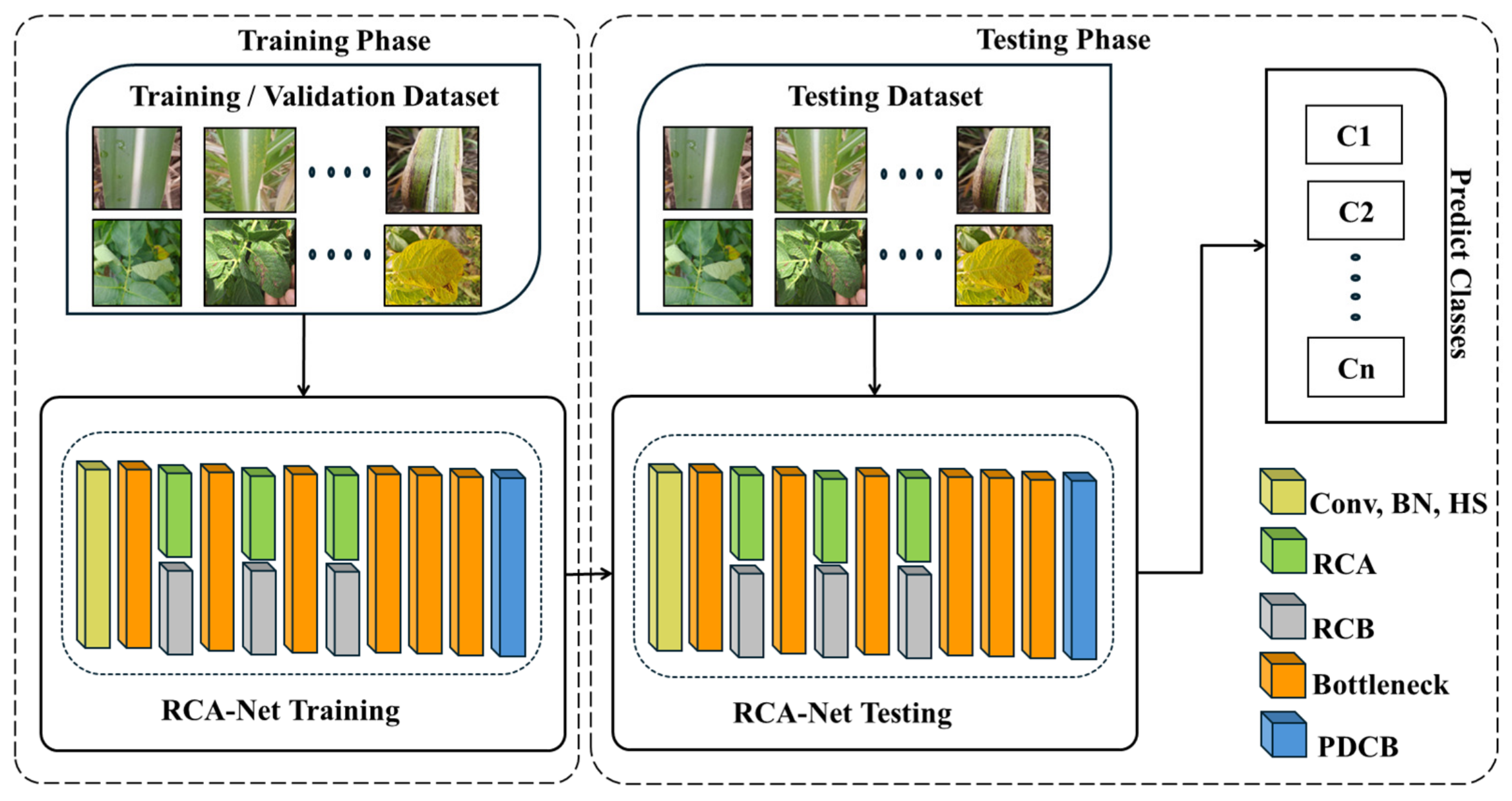
3.1. Workflow Overview of the Proposed Method
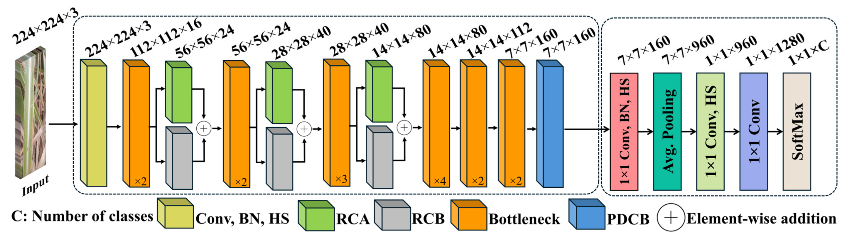
3.2. Structure of RCA-Net
3.2.1. RCA
3.2.2. RCB
3.2.3. PDCB
4. Experimental Results and Analysis
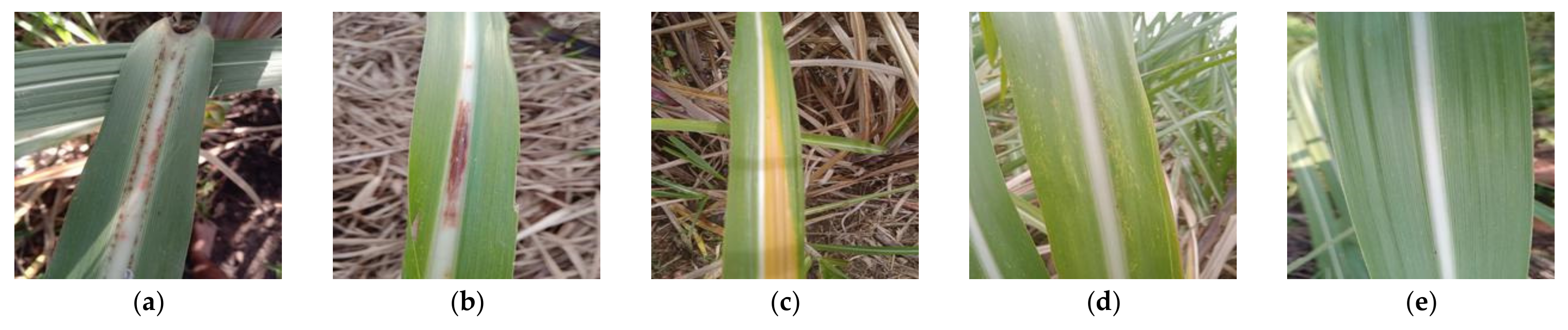
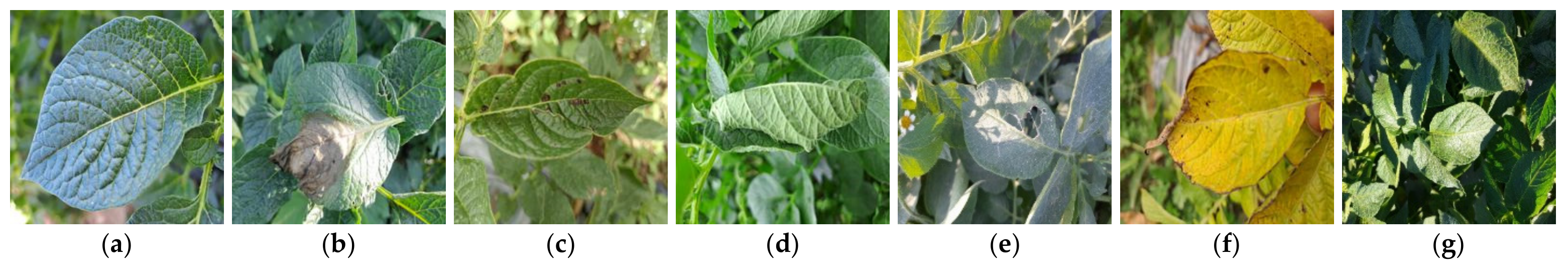
4.1. Experimental Dataset and Setup
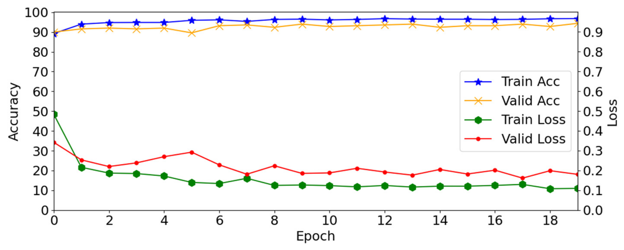
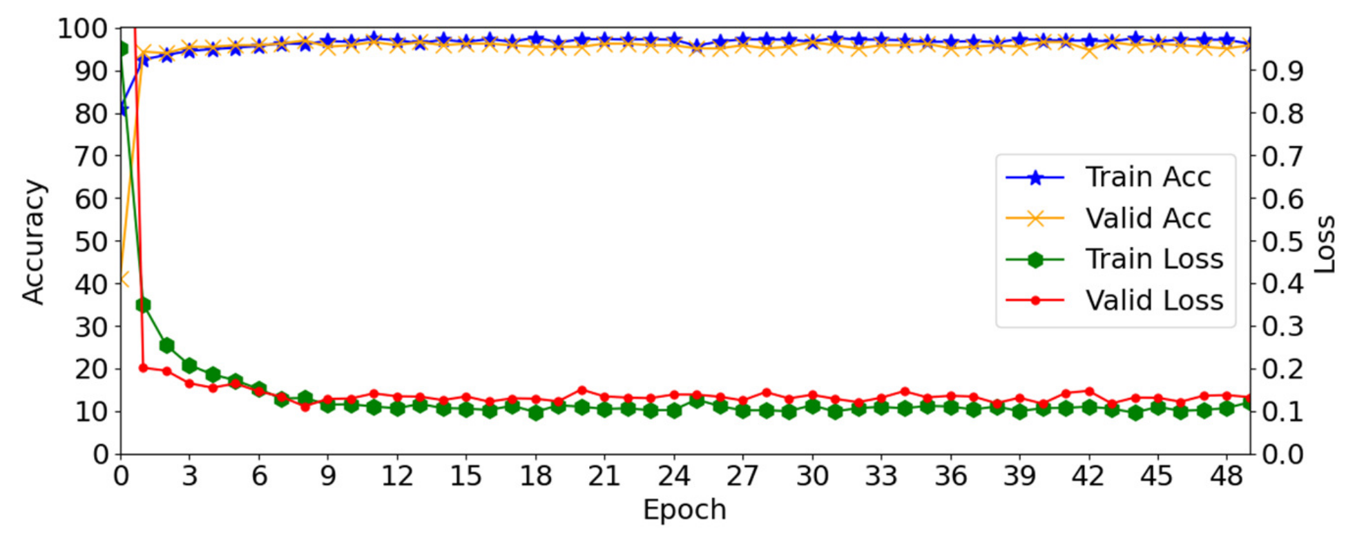
4.2. Training of the Proposed Method
4.3. Testing of Proposed Method
4.3.1. Evaluation Metrics
| Algorithm 1: FD estimation pseudo-code [46] |
| Input: Img: Binarized grad-cam activated image from the output of RCA-Net |
| Output: Fractal dimension (FD) |
| 1: Fix the box to maximum dimensions nearest to the power of 2 = 2^[log(max(size(Img)))/log2] |
| 2: Adjust the size by padding of the Img if its dimensions are less than if size(Img) < size(): padding(Img) = end |
| 3: Initialize the number of boxes b = zeros (1, + 1) |
| 4: Calculate the number of boxes M() until the last pixel of diseased region b( + 1) = sum(Img(:)) |
| 5: Decrease the size of the box by dividing by 2 and again calculate M() while |
| 6: Perform calculation of log(M( for each value of |
| 7: Fit a straight line to [(log(M()] using least square regression: FD = slope of fitted line |
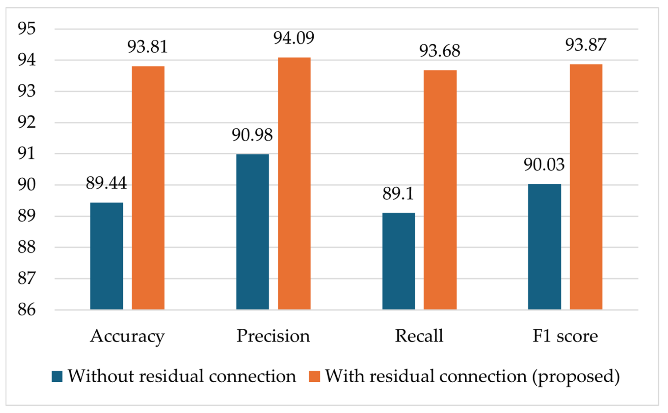
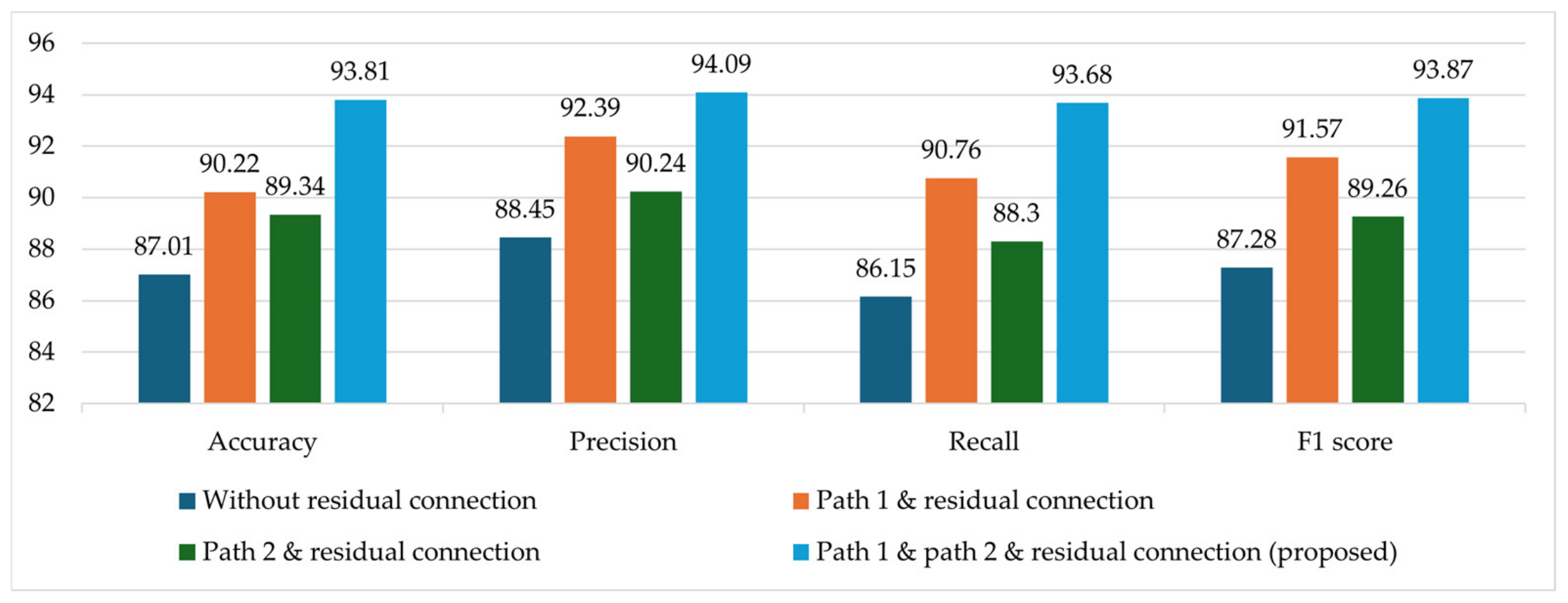
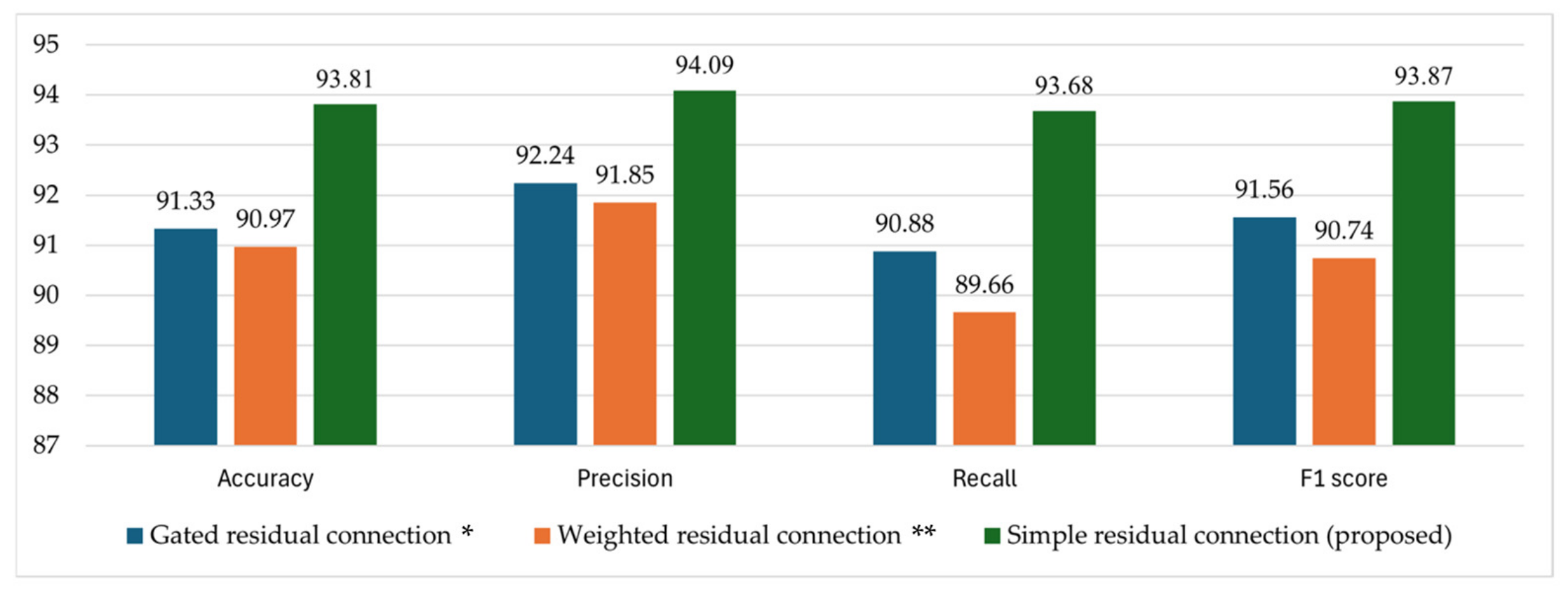
4.3.2. Ablation Studies
4.3.3. Comparison of the RCA-Net with SOTA Models
4.3.4. Comparisons of Processing Time and Model Complexity
5. Discussions
5.1. Confusion Matrix
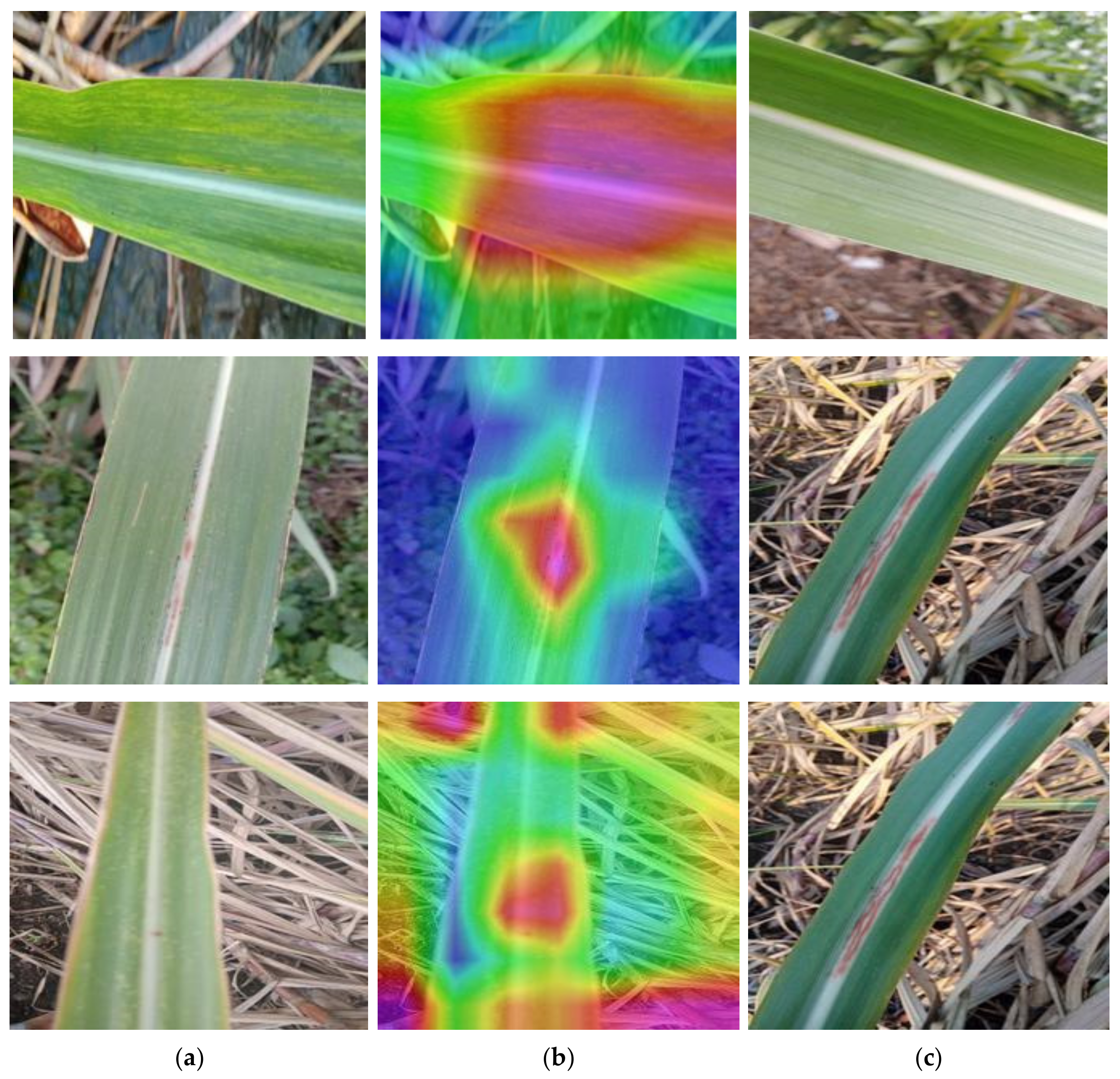
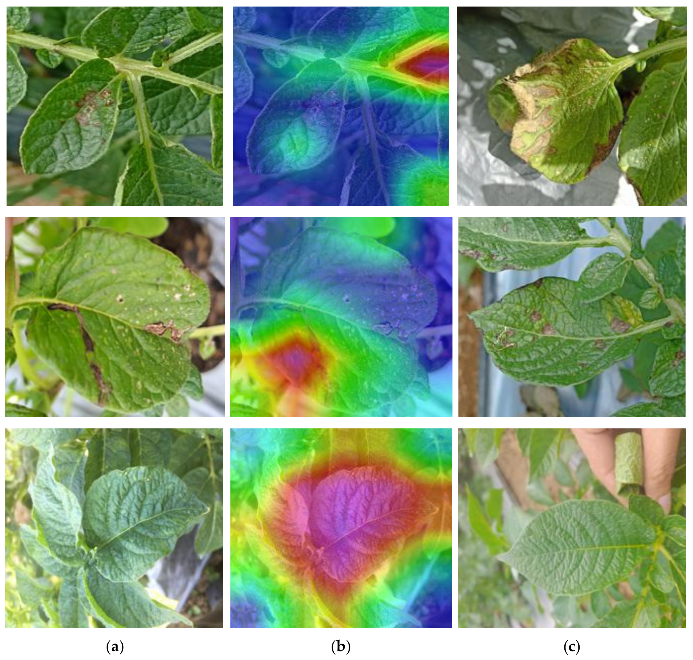
5.2. Grad-CAM
5.3. Evaluating RCA-Net’s Performance by FD Estimation
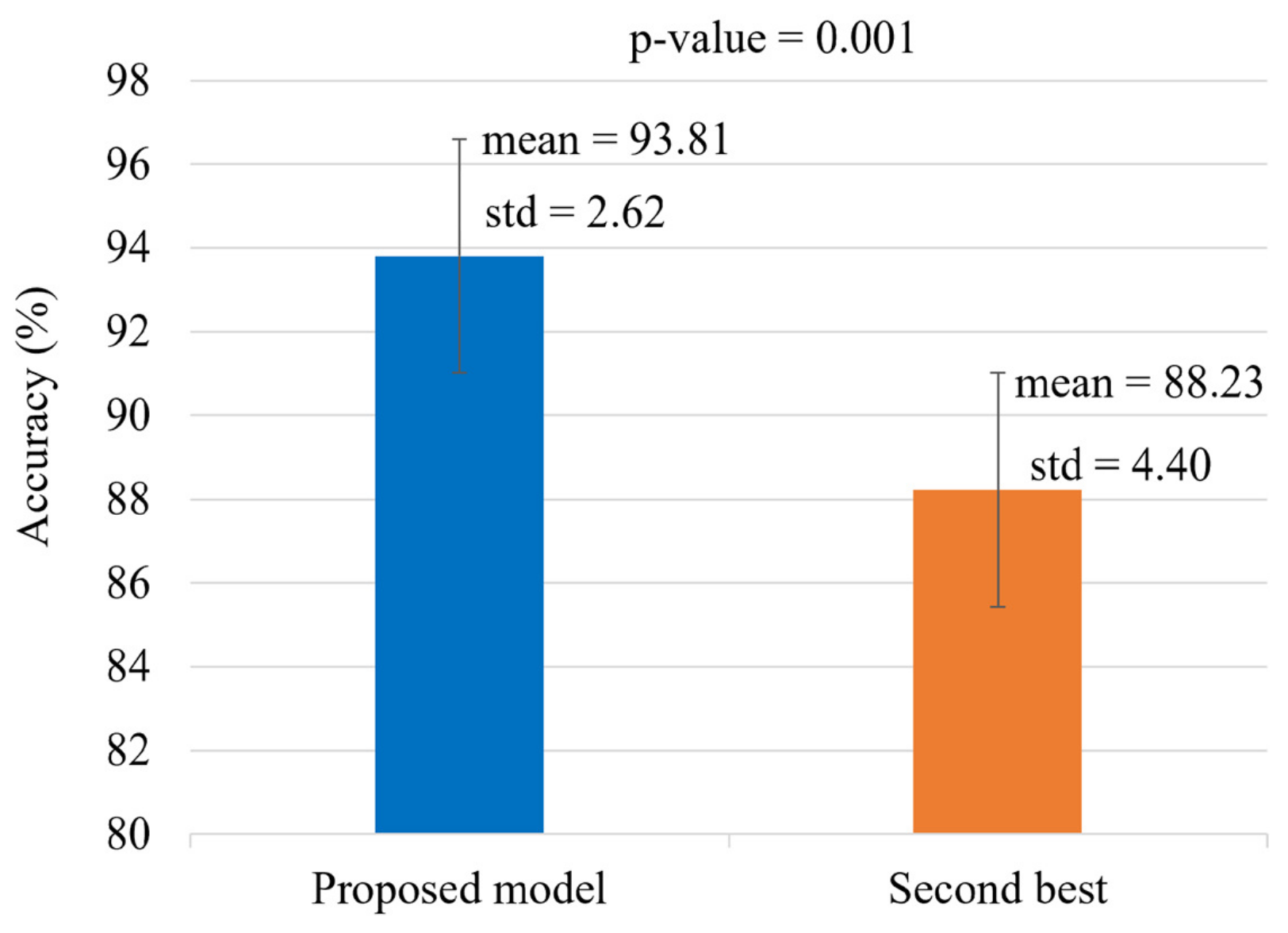
5.4. Statistical Analysis
6. Conclusions
Author Contributions
Funding
Data Availability Statement
Conflicts of Interest
References
- Tian, H.; Wang, T.; Liu, Y.; Qiao, X.; Li, Y. Computer vision technology in agricultural automation—A review. Inf. Process. Agric. 2020, 7, 1–19. [Google Scholar] [CrossRef]
- Sharma, A.; Jain, A.; Gupta, P.; Chowdary, V. Machine learning applications for precision agriculture: A comprehensive review. IEEE Access 2020, 9, 4843–4873. [Google Scholar] [CrossRef]
- Iqbal, Z.; Khan, M.A.; Sharif, M.; Shah, J.H.; ur Rehman, M.H.; Javed, K. An automated detection and classification of citrus plant diseases using image processing techniques: A review. Comput. Electron. Agric. 2018, 153, 12–32. [Google Scholar] [CrossRef]
- Ampatzidis, Y.; De Bellis, L.; Luvisi, A. iPathology: Robotic applications and management of plants and plant diseases. Sustainability 2017, 9, 1010. [Google Scholar] [CrossRef]
- Cruz, A.; Ampatzidis, Y.; Pierro, R.; Materazzi, A.; Panattoni, A.; De Bellis, L.; Luvisi, A. Detection of grapevine yellows symptoms in Vitis vinifera L. with artificial intelligence. Comput. Electron. Agric. 2019, 157, 63–76. [Google Scholar] [CrossRef]
- Shirahatti, J.; Patil, R.; Akulwar, P. A survey paper on plant disease identification using machine learning approach. In Proceedings of the 3rd International Conference on Communication and Electronics Systems (ICCES), Coimbatore, India, 15–16 October 2018. [Google Scholar]
- Mohyuddin, G.; Khan, M.A.; Haseeb, A.; Mahpara, S.; Waseem, M.; Saleh, A.M. Evaluation of Machine Learning approaches for precision Farming in Smart Agriculture System-A comprehensive Review. IEEE Access 2024, 12, 60155–60184. [Google Scholar] [CrossRef]
- Delfani, P.; Thuraga, V.; Banerjee, B.; Chawade, A. Integrative approaches in modern agriculture: IoT, ML and AI for disease forecasting amidst climate change. Precis. Agric. 2024, 25, 2589–2613. [Google Scholar] [CrossRef]
- Naseer, A.; Shmoon, M.; Shakeel, T.; Ur Rehman, S.; Ahmad, A.; Gruhn, V. A Systematic Literature Review of the IoT in Agriculture-Global Adoption, Innovations, Security Privacy Challenges. IEEE Access 2024, 12, 60986–61021. [Google Scholar] [CrossRef]
- RCA-Net. Available online: https://github.com/mhamza92/RCA-Net (accessed on 15 April 2025).
- Narla, V.L.; Suresh, G. Multiple feature-based tomato plant leaf disease classification using SVM classifier. In Machine Learning, Image Processing, Network Security, and Data Sciences; Doriya, R., Soni, B., Shukla, A., Gao, X.-Z., Eds.; Lecture Notes in Electrical Engineering; Springer Nature: Singapore, 2023; Volume 946, pp. 443–455. [Google Scholar] [CrossRef]
- Applalanaidu, M.V.; Kumaravelan, G. A review of machine learning approaches in plant leaf disease detection and classification. In Proceedings of the 3rd International Conference on Intelligent Communication Technologies and Virtual Mobile Networks (ICICV), Tirunelveli, India, 4–5 February 2021. [Google Scholar] [CrossRef]
- Hossain, E.; Hossain, M.F.; Rahaman, M.A. A color and texture based approach for the detection and classification of plant leaf disease using KNN classifier. In Proceedings of the International Conference on Electrical, Computer and Communication Engineering (ECCE), Cox’sBazar, Bangladesh, 7–9 February 2019; IEEE: Piscataway, NJ, USA, 2019. [Google Scholar] [CrossRef]
- Mokhtar, U.; El Bendary, N.; Hassenian, A.E.; Emary, E.; Mahmoud, M.A.; Hefny, H.; Tolba, M.F. SVM-based detection of tomato leaves diseases. In Proceedings of the 7th IEEE International Conference Intelligent Systems IS, Warsaw, Poland, 24–26 September 2014. [Google Scholar] [CrossRef]
- Bhagat, M.; Kumar, D. Efficient feature selection using BoWs and SURF method for leaf disease identification. Multimed. Tools Appl. 2023, 82, 28187–28211. [Google Scholar] [CrossRef]
- Pantazi, X.E.; Moshou, D.; Tamouridou, A.A. Automated leaf disease detection in different crop species through image features analysis and One Class Classifiers. Comput. Electron. Agric. 2019, 156, 96–104. [Google Scholar] [CrossRef]
- Pandey, A.; Jain, K. An intelligent system for crop identification and classification from UAV images using conjugated dense convolutional neural network. Comput. Electron. Agric. 2022, 192, 106543. [Google Scholar] [CrossRef]
- Paymode, A.S.; Malode, V.B. Transfer learning for multi-crop leaf disease image classification using convolutional neural network VGG. Artif. Intell. Agric. 2022, 6, 23–33. [Google Scholar] [CrossRef]
- Agarwal, M.; Abhishek, S.; Siddhartha, A.; Amit, S.; Suneet, G. ToLeD: Tomato leaf disease detection using convolution neural network. Procedia Comput. Sci. 2020, 167, 293–301. [Google Scholar] [CrossRef]
- Atila, Ü.; Uçar, M.; Akyol, K.; Uçar, E. Plant leaf disease classification using EfficientNet deep learning model. Ecol. Inform. 2021, 61, 101182. [Google Scholar] [CrossRef]
- Hughes, D.; Salathé, M. An open access repository of images on plant health to enable the development of mobile disease diagnostics. arXiv 2016, arXiv:1511.08060. [Google Scholar]
- Esgario, J.G.; Krohling, R.A.; Ventura, J.A. Deep learning for classification and severity estimation of coffee leaf biotic stress. Comput. Electron. Agric. 2020, 169, 105162. [Google Scholar] [CrossRef]
- Nag, A.; Chanda, P.R.; Nandi, S. Mobile app-based tomato disease identification with fine-tuned convolutional neural networks. Comput. Electr. Eng. 2023, 112, 108995. [Google Scholar] [CrossRef]
- Zhao, Y.; Li, Y.; Wu, N.; Xu, X. Neural network based on convolution and self-attention fusion mechanism for plant leaves disease recognition. Crop Prot. 2024, 180, 106637. [Google Scholar] [CrossRef]
- Liu, J.; Wang, X. Plant diseases and pests detection based on deep learning: A review. Plant Methods 2021, 17, 1–18. [Google Scholar] [CrossRef]
- Madhavan, M.V.; Thanh, D.N.H.; Khamparia, A.; Pande, S.; Malik, R.; Gupta, D. Recognition and classification of pomegranate leaves diseases by image processing and machine learning techniques. Comput. Mater. Contin. 2021, 66, 2939–2955. [Google Scholar] [CrossRef]
- Zhao, Y.; Zhang, Z.; Wu, N.; Zhang, Z.; Xu, X. MAFDE-DN4: Improved Few-shot plant disease classification method based on Deep Nearest Neighbor Neural Network. Comput. Electron. Agric. 2024, 226, 109373. [Google Scholar] [CrossRef]
- Ding, J.; Zhang, C.; Cheng, X.; Yue, Y.; Fan, G.; Wu, Y.; Zhang, Y. Method for classifying apple leaf diseases based on dual attention and multi-scale feature extraction. Agriculture 2023, 13, 940. [Google Scholar] [CrossRef]
- Wang, P.; Xiong, Y.; Zhang, H. Maize leaf disease recognition based on improved MSRCR and OSCRNet. Crop Prot. 2024, 183, 106757. [Google Scholar] [CrossRef]
- Wang, X.; Wang, Y.; Zhao, J.; Niu, J. ECA-ConvNext: A rice leaf disease identification model based on ConvNext. In Proceedings of the IEEE/CVF Conference on Computer Vision and Pattern Recognition, Vancouver, BC, Canada, 17–24 June 2023. [Google Scholar] [CrossRef]
- Daphal, S.D.; Koli, S.M. Enhancing sugarcane disease classification with ensemble deep learning: A comparative study with transfer learning techniques. Heliyon 2023, 9, e18261. [Google Scholar] [CrossRef] [PubMed]
- Xu, Y.; Shi, Z.; Xie, X.; Chen, Z.; Xie, Z. Residual channel attention fusion network for road extraction based on remote sensing images and GPS trajectories. IEEE J. Sel. Top. Appl. Earth Obs. Remote Sens. 2024, 17, 8358–8369. [Google Scholar] [CrossRef]
- Wang, F.; Jiang, M.; Qian, C.; Yang, S.; Li, C.; Zhang, H.; Wang, X.; Tang, X. Residual attention network for image classification. In Proceedings of the IEEE/CVF Conference on Computer Vision and Pattern Recognition (CVPR), Honolulu, HI, USA, 21–26 July 2017; pp. 3156–3164. [Google Scholar] [CrossRef]
- Howard, A.; Sandler, M.; Chu, G.; Chen, L.C.; Chen, B.; Tan, M.; Wang, W.; Zhu, Y.; Pang, R.; Vasudevan, V.; et al. Searching for mobilenetv3. In Proceedings of the IEEE/CVF International Conference on Computer Vision (ICCV), Seoul, Republic of Korea, 17 October–2 November 2019. [Google Scholar] [CrossRef]
- MobilenetV3. Available online: https://github.com/xiaolai-sqlai/mobilenetv3.git (accessed on 10 January 2024).
- Hu, J.; Shen, L.; Sun, G. Squeeze-and-excitation networks. In Proceedings of the IEEE Conference on Computer Vision and Pattern Recognition (CVPR), Salt Lake City, UT, USA, 18–23 June 2018. [Google Scholar] [CrossRef]
- Life, S.; Szegedy, C. Batch normalization: Accelerating deep network training by reducing internal covariate shift. In Proceedings of the International Conference of Machine Learning (ICML), Lille, France, 6–11 July 2015. [Google Scholar] [CrossRef]
- Yu, F.; Koltun, V. Multi-scale context aggregation by dilated convolutions. In Proceedings of the International Conference on Learning Representation (ICLR), San Juan, Puerto Rico, 2–4 May 2016. [Google Scholar] [CrossRef]
- Daphal, S.D.; Koli, S.M. Sugarcane leaf disease dataset. Mendeley Data 2022, 1. [Google Scholar] [CrossRef]
- Shabrina, N.H.; Indarti, S.; Maharani, R.; Kristiyanti, D.A.; Prastomo, N. A novel dataset of potato leaf disease in uncontrolled environment. Data Brief 2024, 52, 109955. [Google Scholar] [CrossRef]
- NVIDIA GeForce GTX 1070. Available online: https://www.nvidia.com/en-us/geforce/10-series/ (accessed on 12 December 2023).
- Paszke, A.; Gross, S.; Massa, F.; Lerer, A.; Bradbury, J.; Chanan, G.; Killeen, T.; Lin, Z.; Gimelshein, N.; Antiga, L.; et al. PyTorch: An imperative style, high-performance deep learning library. In Proceedings of the Conference of Advances in Neural Information Processing Systems 32 (NeurIPS), Vancouver, BC, Canada, 8–14 December 2019. [Google Scholar] [CrossRef]
- Pham, T.D.; Lee, Y.W.; Park, C.; Park, K.R. Deep Learning-Based Detection of Fake Multinational Banknotes in a Cross-Dataset Environment Utilizing Smartphone Cameras for Assisting Visually Impaired Individuals. Mathematics 2022, 10, 1616. [Google Scholar] [CrossRef]
- Sokolova, M.; Lapalme, G. A systematic analysis of performance measures for classification tasks. Inf. Process. Manag. 2009, 45, 427–437. [Google Scholar] [CrossRef]
- Akram, R.; Hong, J.S.; Kim, S.G.; Sultan, H.; Usman, M.; Gondal, H.A.H.; Tariq, M.H.; Ullah, N.; Park, K.R. Crop and weed segmentation and fractal dimension estimation using small training data in heterogeneous data environment. Fractal Fract. 2024, 8, 285. [Google Scholar] [CrossRef]
- Sultan, H.; Ullah, N.; Hong, J.S.; Kim, S.G.; Lee, D.C.; Jung, S.Y.; Park, K.R. Estimation of fractal dimension and segmentation of brain tumor with parallel features aggregation network. Fractal Fract. 2024, 8, 357. [Google Scholar] [CrossRef]
- Kim, S.G.; Hong, J.S.; Kim, J.S.; Park, K.R. Estimation of fractal dimension and detection of fake finger-vein images for finger-vein recognition. Fractal Fract. 2024, 8, 646. [Google Scholar] [CrossRef]
- Chen, Y.; Wang, Y.; Li, X. Fractal dimensions derived from spatial allometric scaling of urban form. Chaos Solitons Fractals 2019, 126, 122–134. [Google Scholar] [CrossRef]
- Wu, J.; Jin, X.; Mi, S.; Tang, J. An Effective Method to Compute the Box-counting Dimension Based on the Mathematical Definition and Intervals. Results Eng. 2020, 6, 100106. [Google Scholar] [CrossRef]
- Wu, J.; Xie, D.; Yi, S.; Yin, S.; Hu, D.; Li, Y.; Wang, Y. Fractal Study of the Development Law of Mining Cracks. Fractal Fract. 2023, 7, 696. [Google Scholar] [CrossRef]
- Cheng, J.; Chen, Q.; Huang, X. An algorithm for crack detection, segmentation, and fractal dimension estimation in low-light environments by fusing fft and convolutional neural network. Fractal Fract. 2023, 7, 820. [Google Scholar] [CrossRef]
- Savarese, P.H.; Mazza, L.O.; Figueiredo, D.R. Learning identity mappings with residual gates. arXiv 2016, arXiv:1611.01260. [Google Scholar] [CrossRef]
- Shen, F.; Gan, R.; Zeng, G. Weighted residuals for very deep networks. In Proceedings of the 3rd International Conference of System and Informatics (ICSAI), Shanghai, China, 19–21 November 2016. [Google Scholar] [CrossRef]
- Yao, J.; Wang, D.; Hu, H.; Xing, W.; Wang, L. ADCNN: Towards learning adaptive dilation for convolutional neural networks. Pattern Recognit. 2022, 123, 108369. [Google Scholar] [CrossRef]
- Paul, S.G.; Biswas, A.A.; Saha, A.; Zulfikar, M.S.; Ritu, N.A.; Zahan, I.; Rahman, M.; Islam, M.A. A real-time application-based convolutional neural network approach for tomato leaf disease classification. Array 2023, 19, 100313. [Google Scholar] [CrossRef]
- Paul, H.; Udayangani, H.; Umesha, K.; Lankasena, N.; Liyanage, C.; Thambugala, K. Maize leaf disease detection using convolutional neural network: A mobile application based on pre-trained VGG16 architecture. N. Z. J. Crop Hortic. Sci. 2025, 53, 367–383. [Google Scholar] [CrossRef]
- Zhang, R.; Zhu, Y.; Ge, Z.; Mu, H.; Qi, D.; Ni, H. Transfer learning for leaf small dataset using improved ResNet50 network with mixed activation functions. Forests 2022, 13, 2072. [Google Scholar] [CrossRef]
- Sutaji, D.; Yıldız, O. LEMOXINET: Lite ensemble MobileNetV2 and Xception models to predict plant disease. Ecol. Inform. 2022, 70, 101698. [Google Scholar] [CrossRef]
- Srivastava, M.; Meena, J. Plant leaf disease detection and classification using modified transfer learning models. Multimed. Tools Appl. 2024, 83, 38411–38441. [Google Scholar] [CrossRef]
- Adnan, F.; Awan, M.J.; Mahmoud, A.; Nobanee, H.; Yasin, A.; Zain, A.M. EfficientNetB3-adaptive augmented deep learning (AADL) for multi-class plant disease classification. IEEE Access 2023, 11, 85426–85440. [Google Scholar] [CrossRef]
- Bi, C.; Xu, S.; Hu, N.; Zhang, S.; Zhu, Z.; Yu, H. Identification method of corn leaf disease based on improved Mobilenetv3 model. Agronomy 2023, 13, 300. [Google Scholar] [CrossRef]
- Li, H.; Qi, M.; Du, B.; Li, Q.; Gao, H.; Yu, J.; Bi, C.; Yu, H.; Liang Ye, G.; Tang, Y. Maize disease classification system design based on improved ConvNeXt. Sustainability 2023, 15, 14858. [Google Scholar] [CrossRef]
- Ji, Z.; Bao, S.; Chen, M.; Wei, L. ICS-ResNet: A Lightweight Network for Maize Leaf Disease Classification. Agronomy 2024, 14, 1587. [Google Scholar] [CrossRef]
- Zhou, H.; Chen, J.; Niu, X.; Dai, Z.; Qin, L.; Ma, L.; Li, J.; Su, Y.; Wu, Q. Identification of leaf diseases in field crops based on improved ShuffleNetV2. Front. Plant Sci. 2024, 15, 1342123. [Google Scholar] [CrossRef]
- NVIDIA Jetson TX2 Module. Available online: https://developer.nvidia.com/embedded/jetson-tx2 (accessed on 10 May 2024).
- Confusion Matrix. Available online: https://en.wikipedia.org/wiki/Confusion_matrix (accessed on 5 January 2024).
- Selvaraju, R.R.; Cogswell, M.; Das, A.; Vedantam, R.; Parikh, D.; Batra, D. Grad-cam: Visual explanations from deep networks via gradient-based localization. In Proceedings of the IEEE International Conference on Computer Vision (ICCV), Seoul, Republic of Korea, 27 October–2 November 2019. [Google Scholar] [CrossRef]
- Student’s T-Test. Available online: http://en.wikipedia.org/wiki/Students%27s_t-test (accessed on 16 June 2024).
- Cohen, J. A power primer. Psychol. Bull. 1992, 112, 155–159. [Google Scholar] [CrossRef]


| Categories | Method | Dataset | Strengths | Limitations | |
|---|---|---|---|---|---|
| Disease classification of images with simple background | ML-based | GLCM texture features and KNN-based classification [12] | - Arkansas plant disease dataset - Reddit-plant leaf disease dataset | - High accuracy - Texture features can be extracted effectively | KNN cannot easily adapt to various changes in a new and untrained pattern |
| BoWs and SVM classifier are used along with the SURF technique for feature extraction [14] | Tomato, potato, and pepper dataset | Feature reduction makes the model robust | Both the SVM and SURF techniques increase computational complexity | ||
| LBP feature extractor and one-class SVM [15] | Vine leaf dataset | - One class classifier reduces the complexity and cost of obtaining labeled data - It learns dynamically from newly added images and expands its recognition ability | The conflict resolution algorithm impacts the model’s interpretability and transparency | ||
| GLCM and SVM-based detection of tomato leaves disease [13] | Self-collected tomato leaves dataset | - GLCM enhances the ability to differentiate between the classes - SVM with different classes offers robustness and flexibility | Appropriate kernel selection is time-consuming | ||
| DL-based | CNN-based VGG-16 for MCLD [17] | - PlantVillage dataset - Self-collected dataset | Performance improved by the hyper-parameter tuning of the VGG-16 network | Additional preprocessing is required | |
| Customized CNN architecture for tomato leaf disease classification [18] | PlantVillage dataset | - Shallow networks and less time required for training - A small number of trainable parameters | - Model trained by 1000 epochs increases the chance of overfitting - Only compared with three pre-trained models | ||
| EfficientNet, VGG-16, ResNet-50 and Inception V3 [19] | PlantVillage dataset | High accuracy was achieved by fine-tuning the hyper-parameters | Computationally complex | ||
| CAST-Net [23] | PlantVillage dataset | An increased receptive field and self-attention mechanism help to increase efficiency | Additional post-processing is required | ||
| ResNet-50, MobileNetV2, VGG-16, etc. [21] | Arabica coffee leaves dataset | Data augmentation increases accuracy and makes the system robust | Only one type of dataset is used | ||
| Disease classification of images with complex background | ML-based | K-means algorithm and multi-class SVM classifier [26] | Pomegranate leaves dataset | - ROI extraction helps the system to extract the important features - Multi-class SVM captures the complexities of leaf patterns more easily | Multi-class SVM requires a long training time |
| DL-based | MAFDE-DNA4 + few shots learning [27] | PlantVillage, FGVC8 and minimageNet dataset | Few-shots learning along with meta-attention mechanism achieved promising results in a complex background. | Requires high-quality labeled images. | |
| MSRCR + OSCRNet [29] | - Maize dataset from 2018 AI challenger crop disease detection competition. - Self collected | - Multi-scale Retinex color restoration. - Self-calibration convolutional residual network | Additional noise was introduced due to color restoration technique. | ||
| ECA-ConvNeXt [30] | Rice leaf disease image sample dataset | The performance is enhanced by the addition of ECA in the ConvNeXt architecture | Increased computational complexity | ||
| Ensemble model [31] | Sugarcane leaf disease dataset | - Better performance even on small datasets - Low amount of time required for the training | Computationally expensive and has a chance of overfitting | ||
| Proposed method (RCA-Net) | - Sugarcane leaf disease dataset - Uncontrolled environment potato leaf dataset | - Robust and computationally effective for disease classification with actual field images - Higher accuracy than SOTA methods | Exhibits low accuracy for images with severely complex backgrounds | ||
| Block | Layer Type | Input | Output | Number of Filters | Stride Info |
|---|---|---|---|---|---|
| Input | Input | 224 × 224 × 3 | - | - | - |
| Conv. Layer_1 | 3 × 3 Conv, BN, HS | 224 × 224 × 3 | 112 × 112 × 16 | 16 | 2 |
| Stage 1 | Bottleneck × 2 | 112 × 112 × 16 | 56 × 56 × 24 | 16, 24 | 1, 2 |
| RCA_1 | 56 × 56 × 24 | 56 × 56 × 24 | 24 | 1 | |
| RCB_1 | 56 × 56 × 24 | 56 × 56 × 24 | 24 | 1 | |
| Addition_1 | 56 × 56 × 24 | 56 × 56 × 24 | 24 | - | |
| Stage 2 | Bottleneck × 2 | 56 × 56 × 24 | 28 × 28 × 40 | 24, 40 | 1, 2 |
| RCA_2 | 28 × 28 × 40 | 28 × 28 × 40 | 40 | 1 | |
| RCB_2 | 28 × 28 × 40 | 28 × 28 × 40 | 40 | 1 | |
| Addition_2 | 28 × 28 × 40 | 28 × 28 × 40 | 40 | - | |
| Stage 3 | Bottleneck × 3 | 28 × 28 × 40 | 14 × 14 × 80 | 40, 40, 80 | 1, 1, 2 |
| RCA_3 | 14 × 14 × 80 | 14 × 14 × 80 | 80 | 1 | |
| RCB_3 | 14 × 14 × 80 | 14 × 14 × 80 | 80 | 1 | |
| Addition_3 | 14 × 14 × 80 | 14 × 14 × 80 | 80 | - | |
| Stage 4 | Bottleneck × 4 | 14 × 14 × 80 | 14 × 14 × 112 | 80, 80, 80, 112 | 1 |
| Stage 5 | Bottleneck × 2 | 14 × 14 × 112 | 7 × 7 × 160 | 112, 160 | 1, 2 |
| Stage 6 | Bottleneck × 2 | 7 × 7 × 160 | 7 × 7 × 160 | 160 | 1 |
| PDCB | 7 × 7 × 160 | 7 × 7 × 160 | 160 | 1 | |
| Conv. Layer_2 | 1 × 1 Conv, BN, HS | 7 × 7 × 160 | 7 × 7 × 960 | 960 | 1 |
| pooling | Avg. pooling | 7 × 7 × 960 | 1 × 1 × 960 | - | 1 |
| FC1 | 1 × 1 Conv, HS | 1 × 1 × 960 | 1 × 1 × 1280 | 1280 | 1 |
| FC2 | 1 × 1 Conv | 1 × 1 × 1280 | 1 × 1 × C | C | - |
| Output | SoftMax | 1 × 1 × C | C | - | - |
| Dataset Name | Classes Name | Number of Images | Total Number of Images | |
|---|---|---|---|---|
| SCLD | Disease | Rust | 514 | 2569 |
| Red Rot | 519 | |||
| Yellow | 505 | |||
| Mosaic | 511 | |||
| Healthy | 520 | |||
| UPLD | Disease | Virus | 532 | 3076 |
| Phytophthora | 347 | |||
| Fungi | 748 | |||
| Bacteria | 569 | |||
| Pest | 611 | |||
| Nematode | 68 | |||
| Healthy | 201 | |||
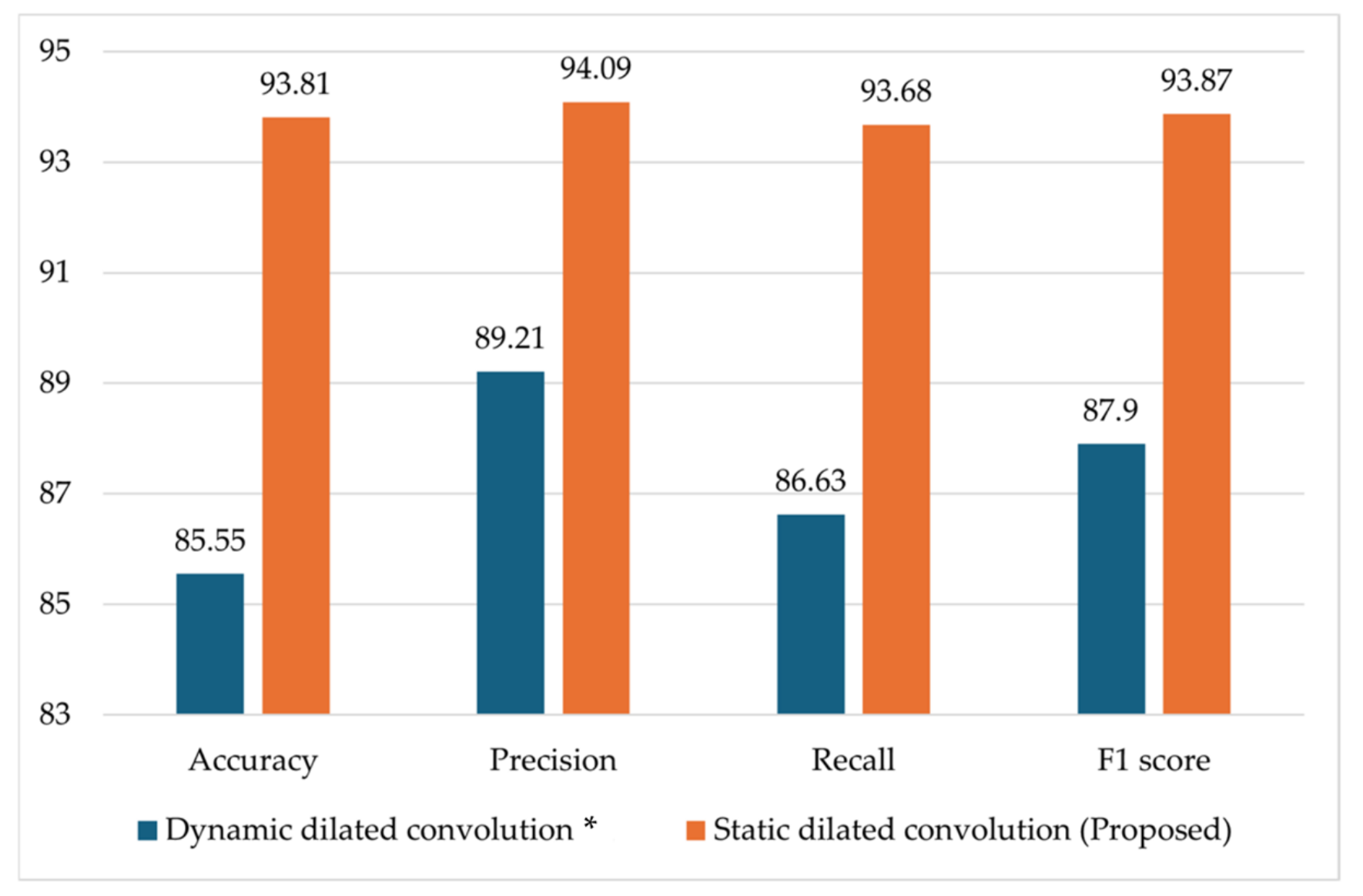
| RCA | RCB | PDCB | Accuracy | Precision | Recall | F1 Score |
|---|---|---|---|---|---|---|
| 84.52 | 87.93 | 84.52 | 86.03 | |||
| ✓ | 88.33 | 88.04 | 86.77 | 87.07 | ||
| ✓ | 87.78 | 88.9 | 86.89 | 88.45 | ||
| ✓ | 86.84 | 87.01 | 86.32 | 86.88 | ||
| ✓ | ✓ | 91.10 | 92.02 | 90.80 | 91.4 | |
| ✓ | ✓ | ✓ | 93.81 | 94.09 | 93.68 | 93.87 |
| Model | SCLD | UPLD | ||||||
|---|---|---|---|---|---|---|---|---|
| Accuracy | Precision | Recall | F1 Score | Accuracy | Precision | Recall | F1 Score | |
| VGG-19 [55] | 70.83 | 58.83 | 57.70 | 58.25 | 75.94 | 74.51 | 75.85 | 75.17 |
| VGG-16 [56] | 64.67 | 70.33 | 64.66 | 67.18 | 59.81 | 60.5 | 59.81 | 60.16 |
| ResNet-50 [57] | 80.64 | 81.21 | 83.60 | 82.38 | 68.17 | 70.06 | 68.17 | 69.10 |
| XceptionNet [58] | 79.17 | 84.36 | 78.79 | 81.47 | 64.45 | 63.13 | 64.14 | 63.63 |
| MobileNetV2 [59] | 81.65 | 85.24 | 80.08 | 82.83 | 76.15 | 71.9 | 76.99 | 74.36 |
| EfficientNet-B3 [60] | 76.91 | 79.74 | 78.01 | 78.85 | 72.35 | 73.78 | 72.35 | 73.08 |
| MobileNetV3-Large [61] | 84.52 | 87.93 | 84.52 | 86.03 | 72.03 | 73.16 | 72.03 | 72.57 |
| ConvNeXt-Tiny [62] | 85.80 | 89.07 | 85.96 | 87.45 | 59.72 | 63.65 | 60.16 | 61.86 |
| DenseNet121 [23] | 79.28 | 84.92 | 79.13 | 81.88 | 59.16 | 60.58 | 59.16 | 59.88 |
| ResNet-101 [63] | 77.12 | 83.57 | 77.17 | 80.78 | 65.21 | 68.92 | 65.26 | 67.04 |
| ShuffleNetV2 [64] | 88.23 | 89.73 | 87.94 | 88.50 | 64.48 | 66.27 | 64.29 | 65.26 |
| ECA-ConvNeXt [30] | 82.34 | 86.46 | 83.12 | 83.77 | 62.78 | 66.13 | 62.52 | 64.28 |
| Ensemble Net [31] | 86.53 | 87.00 | 88.00 | 87.50 | - | - | - | - |
| RCA-Net (proposed) | 93.81 | 94.09 | 93.68 | 93.87 | 78.14 | 75.39 | 78.01 | 76.91 |
| Model | Accuracy | Precision | Recall | F1 Score |
|---|---|---|---|---|
| VGG-19 [55] | 73.97 | 74.71 | 73.80 | 73.24 |
| VGG-16 [56] | 56.27 | 56.97 | 56.27 | 56.57 |
| ResNet-50 [57] | 66.24 | 66.59 | 66.29 | 66.49 |
| XceptionNet [58] | 62.85 | 61.66 | 62.35 | 61.93 |
| MobileNetV2 [59] | 74.03 | 72.88 | 74.79 | 73.82 |
| EfficientNet-B3 [60] | 72.35 | 73.78 | 72.35 | 72.99 |
| MobileNetV3-Large [61] | 70.42 | 70.92 | 70.42 | 70.79 |
| ConvNeXt-Tiny [62] | 65.89 | 68.72 | 65.01 | 66.84 |
| DenseNet121 [23] | 58.52 | 58.52 | 58.52 | 58.52 |
| ResNet-101 [63] | 68.42 | 70.10 | 67.68 | 69.84 |
| ShuffleNetV2 [64] | 69.12 | 68.67 | 68.03 | 68.35 |
| ECA-ConvNeXt [30] | 60.63 | 62.97 | 60.02 | 61.75 |
| RCA-Net (Proposed) | 74.59 | 67.72 | 73.14 | 70.32 |
| Model | Param (M) | FLOPs (G) | Memory Usage (MB) | Inference Time (ms) | |
|---|---|---|---|---|---|
| Desktop | Jetson TX2 | ||||
| VGG-19 [55] | 139.59 | 19.63 | 532.50 | 11.20 | 112.68 |
| VGG-16 [56] | 134.28 | 15.46 | 512.24 | 10.46 | 80.38 |
| ResNet-50 [57] | 23.52 | 4.13 | 89.72 | 8.02 | 26.62 |
| XceptionNet [58] | 22.85 | 8.34 | 88 | 10.14 | 44.28 |
| MobileNetV2 [59] | 2.23 | 0.32 | 8.51 | 7.11 | 11.26 |
| EfficientNet-B3 [60] | 10.70 | 1.01 | 40.83 | 8.21 | 41.1 |
| MobileNetV3-Large [61] | 4.21 | 0.23 | 16.05 | 7.15 | 12.63 |
| ConvNeXt-Tiny [62] | 28.57 | 4.46 | 109.03 | 10.27 | 53.44 |
| DenseNet121 [23] | 6.95 | 2.89 | 30.8 | 8.64 | 31.71 |
| ResNet-101 [63] | 42.51 | 7.86 | 162.16 | 10.20 | 43.17 |
| ShuffleNetV2 [64] | 1.25 | 0.15 | 4.80 | 7.67 | 9.61 |
| ECA-ConvNeXt [30] | 87.51 | 15.35 | 333.99 | 12.78 | 135.96 |
| RCA-Net (proposed) | 5.91 | 0.41 | 22.55 | 7.26 | 12.70 |
| Results | Healthy | Mosaic | Red Rot | Rust | Yellow |
|---|---|---|---|---|---|
| FD | 1.7465 | 1.5591 | 1.3891 | 1.4746 | 1.4707 |
| R2 | 0.998539 | 0.99565 | 0.99162 | 0.99303 | 0.99590 |
| C | 0.999269 | 0.99783 | 0.99580 | 0.99651 | 0.99795 |
Disclaimer/Publisher’s Note: The statements, opinions and data contained in all publications are solely those of the individual author(s) and contributor(s) and not of MDPI and/or the editor(s). MDPI and/or the editor(s) disclaim responsibility for any injury to people or property resulting from any ideas, methods, instructions or products referred to in the content. |
© 2025 by the authors. Licensee MDPI, Basel, Switzerland. This article is an open access article distributed under the terms and conditions of the Creative Commons Attribution (CC BY) license (https://creativecommons.org/licenses/by/4.0/).
Share and Cite
Tariq, M.H.; Sultan, H.; Akram, R.; Kim, S.G.; Kim, J.S.; Usman, M.; Gondal, H.A.H.; Seo, J.; Lee, Y.H.; Park, K.R. Estimation of Fractal Dimensions and Classification of Plant Disease with Complex Backgrounds. Fractal Fract. 2025, 9, 315. https://doi.org/10.3390/fractalfract9050315
Tariq MH, Sultan H, Akram R, Kim SG, Kim JS, Usman M, Gondal HAH, Seo J, Lee YH, Park KR. Estimation of Fractal Dimensions and Classification of Plant Disease with Complex Backgrounds. Fractal and Fractional. 2025; 9(5):315. https://doi.org/10.3390/fractalfract9050315
Chicago/Turabian StyleTariq, Muhammad Hamza, Haseeb Sultan, Rehan Akram, Seung Gu Kim, Jung Soo Kim, Muhammad Usman, Hafiz Ali Hamza Gondal, Juwon Seo, Yong Ho Lee, and Kang Ryoung Park. 2025. "Estimation of Fractal Dimensions and Classification of Plant Disease with Complex Backgrounds" Fractal and Fractional 9, no. 5: 315. https://doi.org/10.3390/fractalfract9050315
APA StyleTariq, M. H., Sultan, H., Akram, R., Kim, S. G., Kim, J. S., Usman, M., Gondal, H. A. H., Seo, J., Lee, Y. H., & Park, K. R. (2025). Estimation of Fractal Dimensions and Classification of Plant Disease with Complex Backgrounds. Fractal and Fractional, 9(5), 315. https://doi.org/10.3390/fractalfract9050315