
A High-Order Fractional Parallel Scheme for Efficient Eigenvalue Computation


Abstract
1. Introduction
- Local convergence depends on an appropriate initial guess.
- Performance deteriorates when eigenvalues are closely spaced.
- Convergence slows or stalls when the derivative of the iterative function approaches zero.
- Sequential computation is inefficient for large-scale problems.
- Fractional-order methods incorporate historical information, enhancing convergence speed and accuracy.
- Modern high-performance architectures reduce computation time.
- Improved numerical stability for complex eigenvalue problems.
- Higher precision without sacrificing efficiency.
- Faster convergence with fewer iterations, reducing computational costs.
- The Caputo derivative of a constant is zero, preserving the classical interpretation of steady-state solutions. In contrast, the Grünwald–Letnikov (GL) derivative yields nonzero values, complicating model interpretation.
- Unlike the GL definition, the Caputo derivative requires only integer-order initial conditions. This allows empirically observed values to be directly incorporated without introducing additional fractional history terms.
- Caputo operators improve the stability and convergence of higher-order iterative solvers by ensuring more consistent kernel behavior. Due to these advantages, the Caputo derivative is almost universally preferred in dynamical models and is particularly well suited for parallel fractional framework schemes.
2. Development and Analysis of the Caputo-Type Fractional Schemes
2.1. Convergence Analysis
2.2. Some Special Cases of the Proposed Fractional Schemes Are Considered
3. Parallel Computing Scheme Construction and Theoretical Convergence
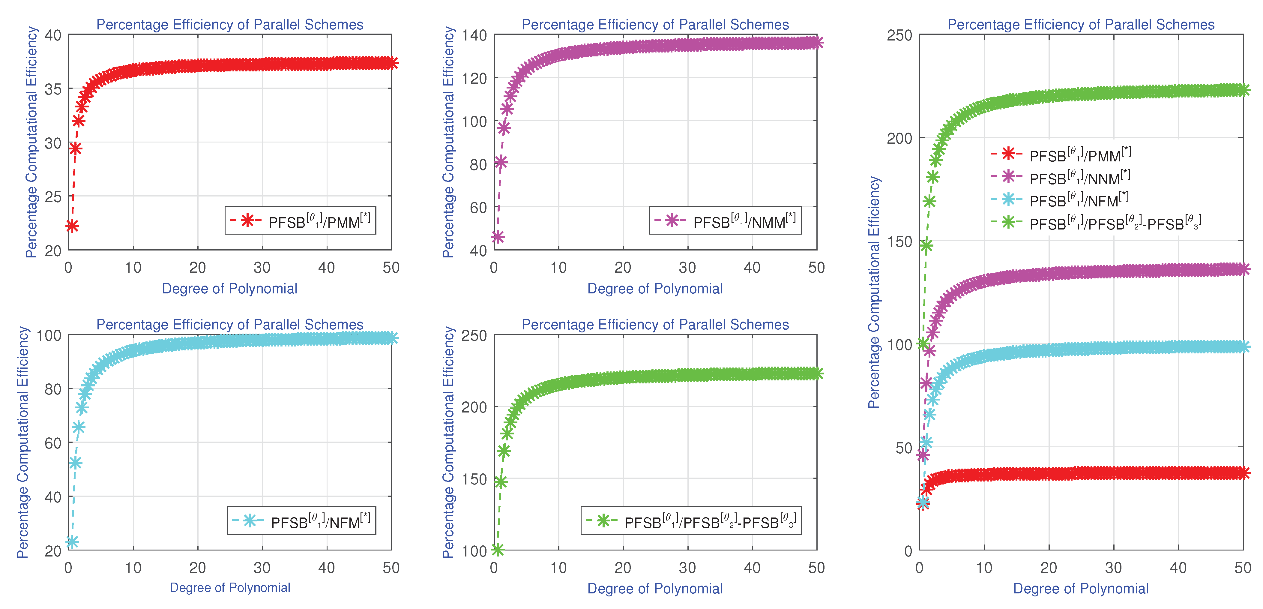
4. Computational Efficiency and Numerical Results
- represents the number of additions and subtractions.
- is the number of multiplications.
- denotes the number of divisions required for a polynomial of degree n.
- Wang–Wu’s parallel scheme () [31] is as follows:
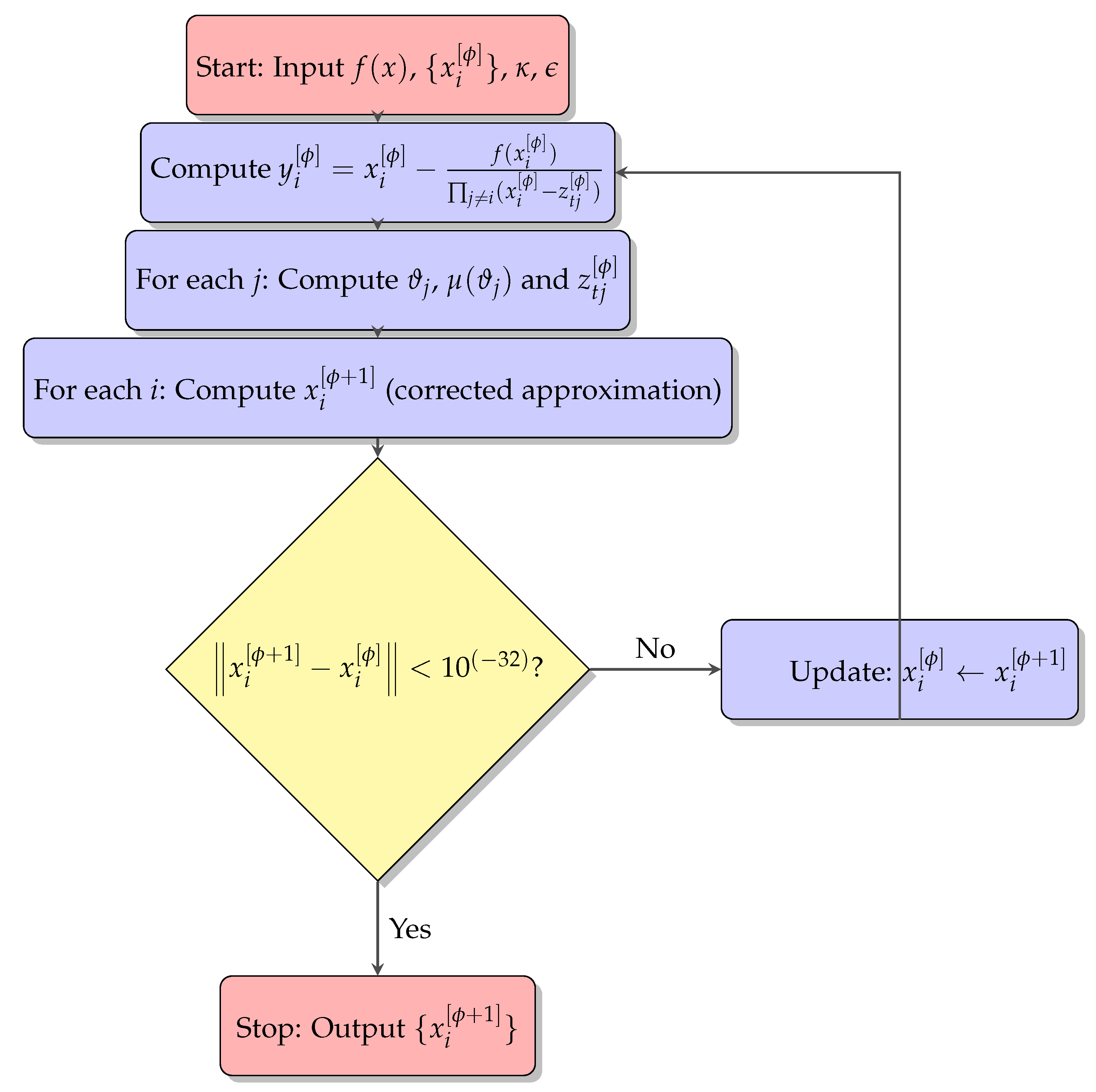
| Algorithm 1: Fractional order parallel scheme for finding all eigenvalues simultaneously. |
|
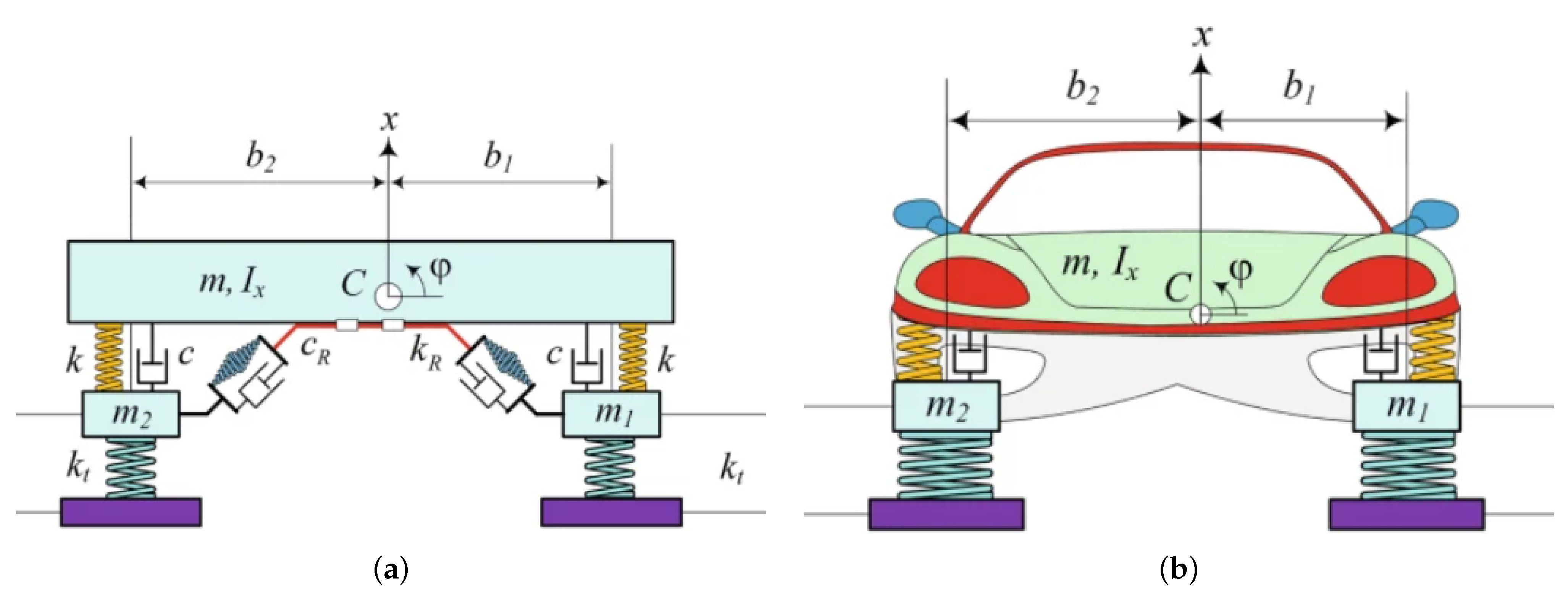
4.1. Mechanical Engineering Model for Automotive Suspension [33]
4.1.1. Model Assumptions
- The system is linear.
- The suspension consists of multiple springs and dampers, each representing a distinct suspension component.
4.1.2. Governing Equations
- is the displacement vector of the masses.
- is the mass matrix.
- is the damping matrix.
- is the stiffness matrix.
- is the external force vector.
4.1.3. Case 1: Two-Degree-of-Freedom (2DOF) System
4.1.4. Analysis of Eigenvalues
- Real eigenvalues: Real eigenvalues indicate stable oscillatory behavior at specific frequencies.
- Complex eigenvalues: The presence of complex eigenvalues suggests damped oscillations, where disturbances gradually decay over time.
4.1.5. Physical Behavioral Interpretation of the Two-Degree-of-Freedom System
- Stable modes: The natural frequencies determine the preferred oscillation modes of the suspension system when disturbed. These modes are crucial for ensuring stability in vehicle dynamics during operation.
- Damping effects: The presence of complex eigenvalues signifies that disturbances will decay over time, leading to a gradual return to equilibrium. This effect is essential for ride comfort, preventing excessive oscillations caused by road irregularities.
- High-frequency response: The highest natural frequency (10.0 Hz) may correspond to the first mode of vibration of the suspension system. This mode is particularly critical for maintaining control and stability at high speeds or during rapid maneuvers.
4.1.6. Case 2: Four-Degree-of-Freedom (4DOF) System
System Parameters
Masses
- kg (car body);
- kg (front-left wheel assembly);
- kg (front-right wheel assembly);
- kg (rear wheel assembly).
Spring Constants
- 80,000 N/m (spring between car body and front axle);
- 60,000 N/m (spring between front axle and ground);
- 60,000 N/m (spring between rear axle and ground).
Damping Coefficients
- 4000 Ns/m (damper between car body and front axle);
- 3000 Ns/m (damper between front axle and ground);
- 3000 Ns/m (damper between rear axle and ground).
Governing Equations
Mass Matrix
Damping Matrix
Stiffness Matrix
4.1.7. Analysis of Eigenvalues for a Four-Degree-of-Freedom Mechanical System
- Stable modes: Real eigenvalues indicate stable modes of oscillation. The frequencies determine how the system naturally oscillates when subjected to disturbances.
- Damped oscillations: Complex eigenvalues signify oscillations that decay over time, representing the damping characteristics of the suspension system. This is crucial for maintaining comfort and ride quality in vehicles.
4.1.8. Physical Interpretation of Eigenvalues in a Four-Degree-of-Freedom System
- Stable modes: The real eigenvalues correspond to natural frequencies ranging from Hz to Hz, where the system exhibits stable oscillations. These modes are critical for ensuring vehicle stability under various loading conditions, particularly when driving over uneven surfaces.
- Damping effects: The presence of complex eigenvalues indicates that the suspension system gradually dissipates energy in response to disturbances, ensuring a smooth return to equilibrium. This characteristic is essential for preventing excessive oscillations that could compromise passenger comfort and vehicle handling.
- Frequency range: The identified natural frequencies define the range of vibrations the suspension system will experience. High-frequency responses (e.g., Hz) correspond to rapid load changes, such as those encountered during cornering or sudden braking.
4.2. Aeroelasticity and Flutter Analysis: Detailed Model and Solution Behavior [35]
4.2.1. Flutter Model Overview
4.2.2. Equations of Motion
- —vertical displacement of the airfoil (bending);
- —angular displacement (torsion);
- m and —mass and moment of inertia of the structure;
- and —damping coefficients;
- and —stiffness coefficients;
- —aerodynamic lift force;
- —aerodynamic pitching moment.
4.2.3. Aerodynamic Forces
- kg—mass per unit length of the wing;
- kg·m2—moment of inertia of the wing;
- Ns/m—damping coefficient for bending;
- Ns·m/rad—damping coefficient for torsion;
- N/m—bending stiffness;
- Nm/rad—torsional stiffness.
- kg/m3—air density;
- m2—wing surface area.
4.2.4. Coupled System and Eigenvalue Problem
4.2.5. Solution Behavior and Physical Interpretation
- Stable regime (below flutter speed): For , the system remains stable. The real parts of all eigenvalues are negative, indicating that oscillations decay over time due to damping. The system naturally returns to equilibrium after disturbances, ensuring structural stability.
- Flutter point (at critical speed): At , the system reaches a marginally stable state. The real part of one pair of eigenvalues approaches zero, meaning that the damping effect vanishes. Oscillations neither grow nor decay, marking the flutter onset speed. Beyond this point, the wing loses its ability to return to a stable state once disturbed.
- Unstable regime (above flutter speed): For , the real part of at least one pair of eigenvalues becomes positive, leading to exponentially growing oscillations. This marks the onset of the flutter regime, where both bending and torsional oscillations increase uncontrollably, potentially causing structural failure unless corrective action, such as reducing airspeed, is taken.
4.3. Limitations of Fractional-Order Parallel Schemes for Eigenvalue Problems
- The techniques can perform worse on matrices with clustered or closely spaced eigenvalues, resulting in slower convergence or instability.
- Optimal convergence and higher accuracy require reasonable initial approximations, which are difficult to produce for nonsymmetric or ill-conditioned matrices.
- The inclusion of fractional-order terms increases computing time, especially for sparse or nontrivially large matrix problems.
- Optimal initialization using fractal analysis is problem-specific and does not provide generic automation.
- Implementation and visualization may require significant computational power and expertise.
5. Conclusions
Author Contributions
Funding
Data Availability Statement
Conflicts of Interest
Notations
| CPU-time | Computational time seconds |
| Max-It | Maximum iterations |
| Max-Err | Maximum error |
| Per-Convergence | Percentage convergence |
| Existing parallel methods | |
| Residual error | |
| Newly developed methods |
Appendix A
Appendix A.1
- Consider the Taylor expansion of around as
- Factoring out , we obtainwhere
- Around , the Caputo-type derivative of is given by
- These expansions are used to analyze the convergence of the methods.
Appendix A.2
Appendix B

| Ran-Test | ||||
|---|---|---|---|---|
| 1 | ||||
| 2 | ||||
| 3 | ||||
| 5 |
| Ran-Test | ||||||||
|---|---|---|---|---|---|---|---|---|
| 1 | ||||||||
| 2 | ||||||||
| 3 | ||||||||
| 5 |
| Ran-Test | ||||
|---|---|---|---|---|
| 1 | ||||
| 2 | ||||
| 3 | ||||
| ⋮ |
References
- Guglielmi, N.; De Marinis, A.; Savostianov, A.; Tudisco, F. Contractivity of neural ODEs: An eigenvalue optimization problem. Math. Comput. 2025. [Google Scholar]
- Meng, F.; Wang, Z.; Zhang, M. Pissa: Principal singular values and singular vectors adaptation of large language models. Adv. Neural Inf. Process. Syst. 2024, 37, 121038–121072. [Google Scholar]
- Ciftci, H.; Hall, R.L.; Saad, N. Construction of exact solutions to eigenvalue problems by the asymptotic iteration method. J. Phys. A Math. Gen. 2005, 38, 1147. [Google Scholar]
- Zhang, Y.; Chen, C.; Ding, T.; Li, Z.; Sun, R.; Luo, Z. Why transformers need adam: A hessian perspective. Adv. Neural Inf. Process. Syst. 2024, 37, 131786–131823. [Google Scholar]
- Ramond, P. The Abel–Ruffini theorem: Complex but not complicated. Am. Math. Mon. 2022, 129, 231–245. [Google Scholar]
- Gidiotis, A.; Tsoumakas, G. A divide-and-conquer approach to the summarization of long documents. IEEE/ACM Trans. Audio Speech Lang. Process. 2020, 28, 3029–3040. [Google Scholar] [CrossRef]
- Goldstine, H.H.; Murray, F.J.; Von Neumann, J. The Jacobi method for real symmetric matrices. J. ACM (JACM) 1959, 6, 59–96. [Google Scholar]
- Fokkema, D.R.; Sleijpen, G.L.; Van der Vorst, H.A. Jacobi–Davidson style QR and QZ algorithms for the reduction of matrix pencils. SIAM J. Sci. Comput. 1998, 20, 94–125. [Google Scholar]
- Lu, Z.; Niu, Y.; Liu, W. Efficient block algorithms for parallel sparse triangular solve. In Proceedings of the 49th International Conference on Parallel Processing, Edmonton, AB, Canada, 17–20 August 2020; pp. 1–11. [Google Scholar]
- Zhang, Z.; Wang, H.; Han, S.; Dally, W.J. Sparch: Efficient architecture for sparse matrix multiplication. In Proceedings of the 2020 IEEE International Symposium on High Performance Computer Architecture (HPCA), San Diego, CA, USA, 22–26 February 2020; pp. 261–274. [Google Scholar]
- Bašić, J.; Blagojevixcx, B.; Baxsxixcx, M.; Sikora, M. Parallelism and Iterative bi-Lanczos Solvers. In Proceedings of the 2021 6th International Conference on Smart and Sustainable Technologies (SpliTech), Split & Bol, Croatia, 8–11 September 2021; pp. 1–6. [Google Scholar]
- Wu, G.; Wei, Y. A Power–Arnoldi algorithm for computing PageRank. Numer. Linear Algebra Appl. 2007, 14, 521–546. [Google Scholar]
- Nourein, A.W. An improvement on Nourein’s method for the simultaneous determination of the zeroes of a polynomial (an algorithm). J. Comput. Appl. Math. 1977, 3, 109–112. [Google Scholar]
- Falcão, M.I.; Miranda, F.; Severino, R.; Soares, M.J. Weierstrass method for quaternionic polynomial root-finding. Math. Methods Appl. Sci. 2018, 41, 423–437. [Google Scholar]
- Kipouros, T.; Jaeggi, D.; Dawes, B.; Parks, G.; Savill, M.A.; Clarkson, P.J. Insight into high-quality aerodynamic design spaces through multi-objective optimization. CMES Comput. Model. Eng. Sci. 2008, 37, 1–23. [Google Scholar]
- Landman, D.; Simpson, J.; Vicroy, D.; Parker, P. Response surface methods for efficient complex aircraft configuration aerodynamic characterization. J. Aircraf. 2007, 44, 1189–1195. [Google Scholar]
- Liu, Y. Bibliometric Analysis of Weather Radar Research from 1945 to 2024: Formations. Develop. Trends Sens. 2024, 24, 3531. [Google Scholar]
- Jajarmi, A.; Baleanu, D. A new iterative method for the numerical solution of high-order non-linear fractional boundary value problems. Front. Phys. 2020, 8, 220. [Google Scholar]
- Sazaklioglu, A.U. An iterative numerical method for an inverse source problem for a multidimensional nonlinear parabolic equation. Appl. Numer. Math. 2024, 198, 428–447. [Google Scholar]
- Akgül, A.; Cordero, A.; Torregrosa, J.R. A fractional Newton method with 2αth-order of convergence and its stability. Appl. Math. Lett. 2019, 98, 344–351. [Google Scholar]
- Batiha, B. Innovative Solutions for the Kadomtsev–Petviashvili Equation via the New Iterative Method. Math. Prob. Eng. 2024, 2024, 5541845. [Google Scholar]
- Weierstrass, K. Neuer Beweis des Satzes, dass jede ganze rationale Function einer Verän derlichen dargestellt werden kann als ein Product aus linearen Functionen derselben Verän derlichen. Sitzungsberichte KöNiglich Preuss. Akad. Der Wiss. Berl. 1981, 2, 1085–1101. [Google Scholar]
- Nedzhibov, G.H. Inverse Weierstrass–Durand–Kerner Iterative Method. Int. J. Appl. Math. 2013, 28, 1258–1264. [Google Scholar]
- Nourein, A.W.M. An improvement on two iteration methods for simultaneous determinationof the zeros of a polynomial. Int. J. Comput. Math. 1977, 6, 241–252. [Google Scholar]
- Zhang, X.; Peng, H.; Hu, G. A high order iteration formula for the simultaneous inclusion of polynomial zeros. Appl. Math. Comput. 2006, 179, 545–552. [Google Scholar]
- Petkovic, M. Iterative Methods for Simultaneous Inclusion of Polynomial Zeros; Springer: Berlin/Heidelberg, Germany, 2006; Volume 1387. [Google Scholar]
- Zein, A. A general family of fifth-order iterative methods for solving nonlinear equations. Eur. J. Pure Appl. Math. 2023, 16, 2323–2347. [Google Scholar]
- Halilu, A.S.; Waziri, M.Y. A transformed double step length method for solving large-scale systems of nonlinear equations. J. Numer. Math. Stochastics 2021, 9, 20–23. [Google Scholar]
- Rafiq, N.; Akram, S.; Shams, M.; Mir, N.A. Computer geometries for finding all real zeros of polynomial equations simultaneously. Comput. Mater. Contin. 2021, 69, 2636–2651. [Google Scholar]
- Petković, M.S.; Petković, L.D.; Džunić, J. On an efficient simultaneous method for finding polynomial zeros. Appl. Math. Lett. 2014, 28, 60–65. [Google Scholar]
- Wang, D.R.; Wu, Y.J. Some modifications of the parallel Halley iteration method and their convergence. Computing 1987, 38, 75–87. [Google Scholar]
- Petković, M.S.; Rančić, L.; Milošević, M. The improved Farmer–Loizou method for finding polynomial zeros. Int. J. Comput. Math. 2012, 89, 499–509. [Google Scholar]
- Gillespie, T. Fundamentals of Vehicle Dynamics; SAE: Warrendale, PA, USA, 2000. [Google Scholar]
- Reimpell, J.; Stoll, H.; Betzler, J. The Automotive Chassis: Engineering Principles; Elsevier: Amsterdam, The Netherlands, 2001. [Google Scholar]
- Prohl, M.A. A general method for calculating critical speeds of flexible rotors. J. Appl. Mech. 1945, 12, A142–A148. [Google Scholar]
- Shams, M.; Carpentieri, B. On highly efficient fractional numerical method for solving nonlinear engineering models. Mathematics 2023, 11, 4914. [Google Scholar] [CrossRef]


| Scheme | ||||||
|---|---|---|---|---|---|---|
| 22.0 | 29.0 | 27.0 | 11.0 | 13.0 | 16.0 | |
| × | 18.0 | 26.0 | 26.0 | 15.0 | 16.0 | 15.0 |
| % Efficiency | 47.12 | 36.34 | 29.33 | 68.89 | 56.41 | 68.99 |
| % Memory Usage | 68.65 | 53.98 | 63.04 | 25.67 | 31.98 | 28.32 |
| Property | Description | |
|---|---|---|
| Matrix Size | (mass, damping, and stiffness matrices) | |
| Polynomial Degree | 4 (due to transformation) | |
| Sparsity | M: | Sparse (only diagonal entries are nonzero) |
| C: | Sparse (few nonzeros) | |
| K: | Sparse (few nonzeros, mostly diagonal and few off-diagonal | |
| Symmetry | Yes | |
| Condition Number | Well conditioned | |
| Eigenvalue Type | Complex |
| Parameter | Range | Effect on Algorithm | Selection Guidance |
|---|---|---|---|
| Controls memory effect and nonlocality. Moderate values improve the convergence region and stability. | Choose for faster convergence. Lower values increase memory and smoothness, influencing stability. | ||
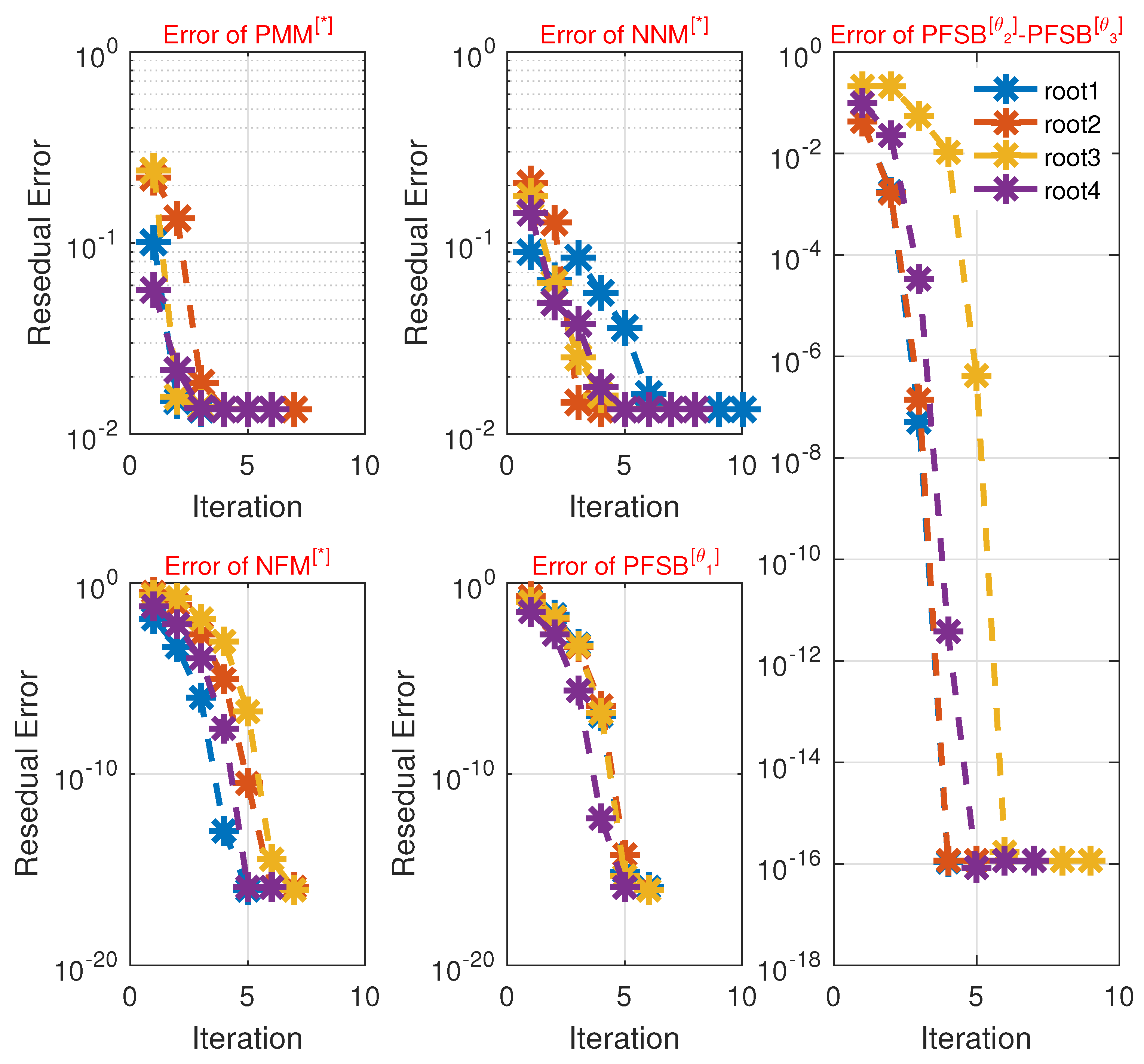
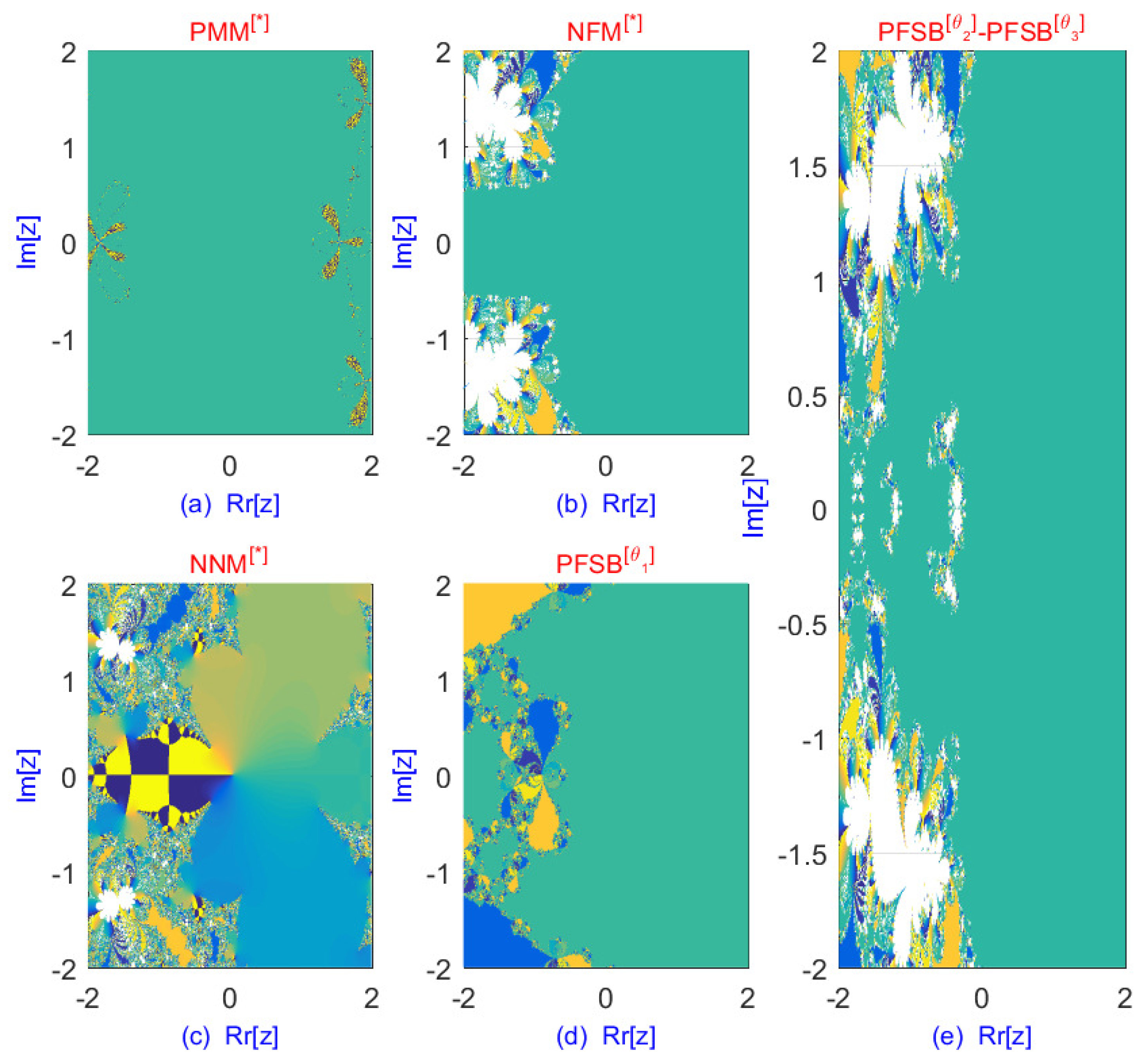
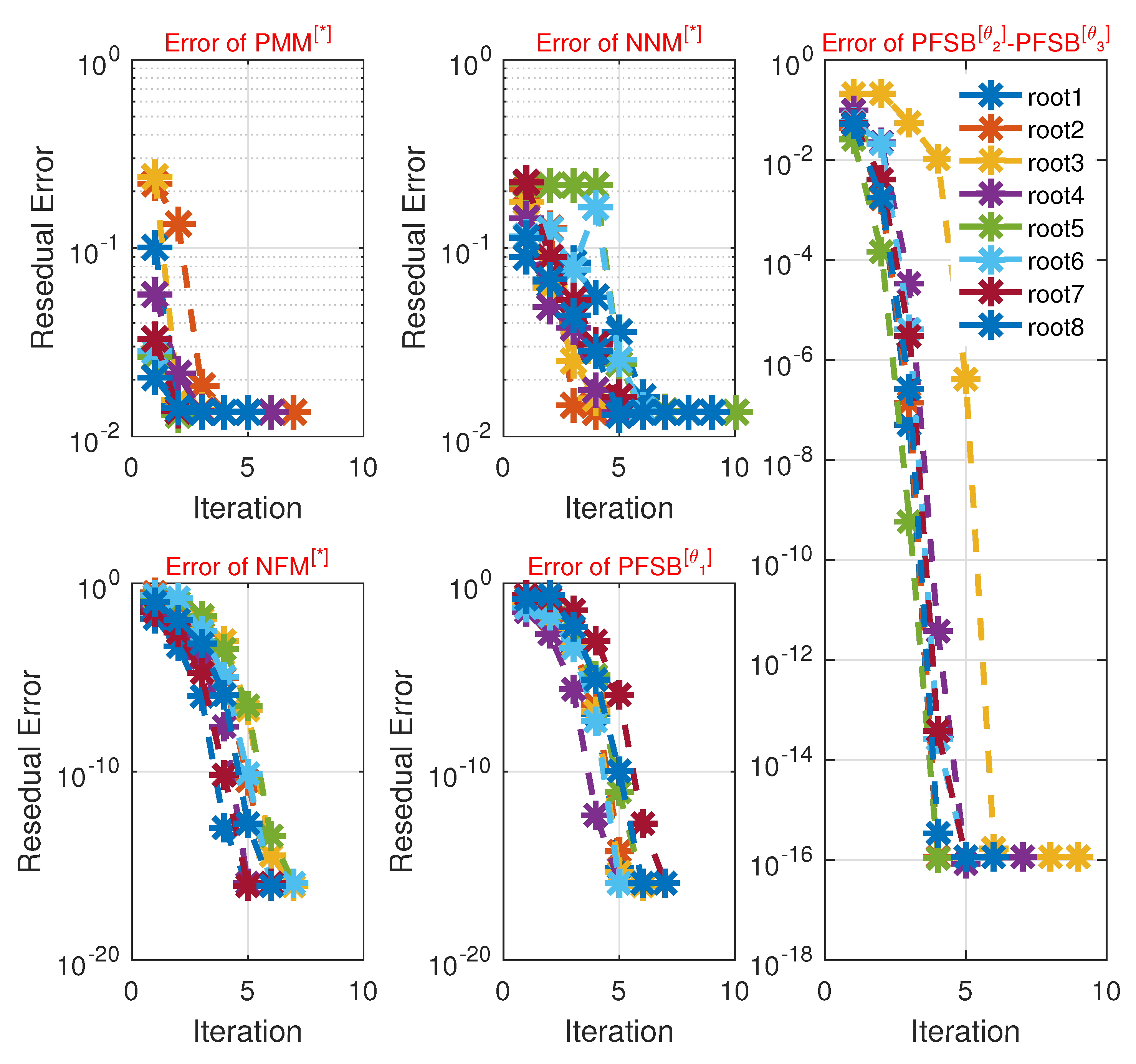
| Figure 4, Figure 5 and Figure 6 illustrate the technique’s enhanced convergence for when compared to existing techniques. | For general problems, we use . For ill-conditioned or stiff eigenvalue problems, we used for improved robustness. |
| Scheme | ||||||
|---|---|---|---|---|---|---|
| Iterations | 27 | 28 | 29 | 29 | 21 | 23 |
| Per-Convergence | 45.346% | 36.465% | 65.51% | 75.01% | 65.768% | 77.453% |
| Method | ||||
|---|---|---|---|---|
| Scheme | ||||||
|---|---|---|---|---|---|---|
| C-Time (s) | 4.5464 | 5.4364 | 3.5465 | 1.2354 | 1.3435 | 1.6343 |
| Memory Usage (%) | 47.876 | 28.123 | 21.002 | 12.432 | 16.657 | 17.456 |
| Scheme | Max-Err | Max-It | Per-Divergence | |
|---|---|---|---|---|
| 22 | 42.0 | 66.1232% | ||
| 21 | 47.0 | 63.3453% | ||
| 20 | 56.0 | 34.4564% | ||
| 16 | 21.0 | 29.4334% | ||
| 11 | 26.0 | 23.5346% | ||
| 8 | 33.0 | 13.3435% |
| Scheme | |||||
|---|---|---|---|---|---|
| CPU−time | |||||
| Max-Err |
| Property | Description | |
|---|---|---|
| Matrix Size | (mass, damping, and stiffness matrices) | |
| Polynomial Degree | 8 (due to transformation) | |
| Sparsity | M: | Sparse (mass matrix is diagonal) |
| C: | Sparse (damping matrices are banded) | |
| K: | Sparse (stiffness matrices are banded) | |
| Symmetry | Yes | |
| Condition Number | ∼; moderately ill-conditioned | |
| Eigenvalue Type | Real and complex conjugate pairs (due to damping) | |
| Scheme | ||||||
|---|---|---|---|---|---|---|
| Iterations | 26 | 27 | 30 | 28 | 20 | 21 |
| Percentage Convergence | 37.546% | 26.654% | 45.771% | 65.432% | 55.004% | 67.987% |
| Method | ||||
|---|---|---|---|---|
| Scheme | ||||||
|---|---|---|---|---|---|---|
| C-Time (s) | 5.7776 | 6.8865 | 6.7555 | 2.3646 | 3.6453 | 2.2436 |
| Memory Usage (%) | 77.436% | 68.998% | 51.565% | 48.002% | 47.070% | 39.986% |
| Scheme | Max-Err | Max-It | Per-Divergence (%) | |
|---|---|---|---|---|
| 22 | 44.0 | 58.1232 | ||
| 21 | 48.0 | 55.7777 | ||
| 20 | 46.0 | 47.9860 | ||
| 16 | 26.0 | 48.2265 | ||
| 11 | 36.0 | 33.0005 | ||
| 8 | 35.0 | 23.1164 |
| Scheme | |||||
|---|---|---|---|---|---|
| CPU−time | |||||
| Max-Err |
| Property | Description | |
|---|---|---|
| Matrix Size | ||
| Polynomial Degree | 4 (due to transformation) | |
| Sparsity | M: | Sparse (only diagonal entries are nonzero) |
| C: | Sparse (few nonzeros) | |
| K: | Sparse (few nonzeros, mostly diagonal and few off-diagonal | |
| Symmetry | Yes | |
| Condition Number | Well conditioned | |
| Eigenvalue Type | Complex |
| Parameter | Range | Effect on Algorithm | Selection Guidance |
|---|---|---|---|
| Controls memory effect and nonlocality. Moderate values improve the convergence region and stability. | Choose for faster convergence. Lower values increase memory and smoothness, influencing stability. | ||
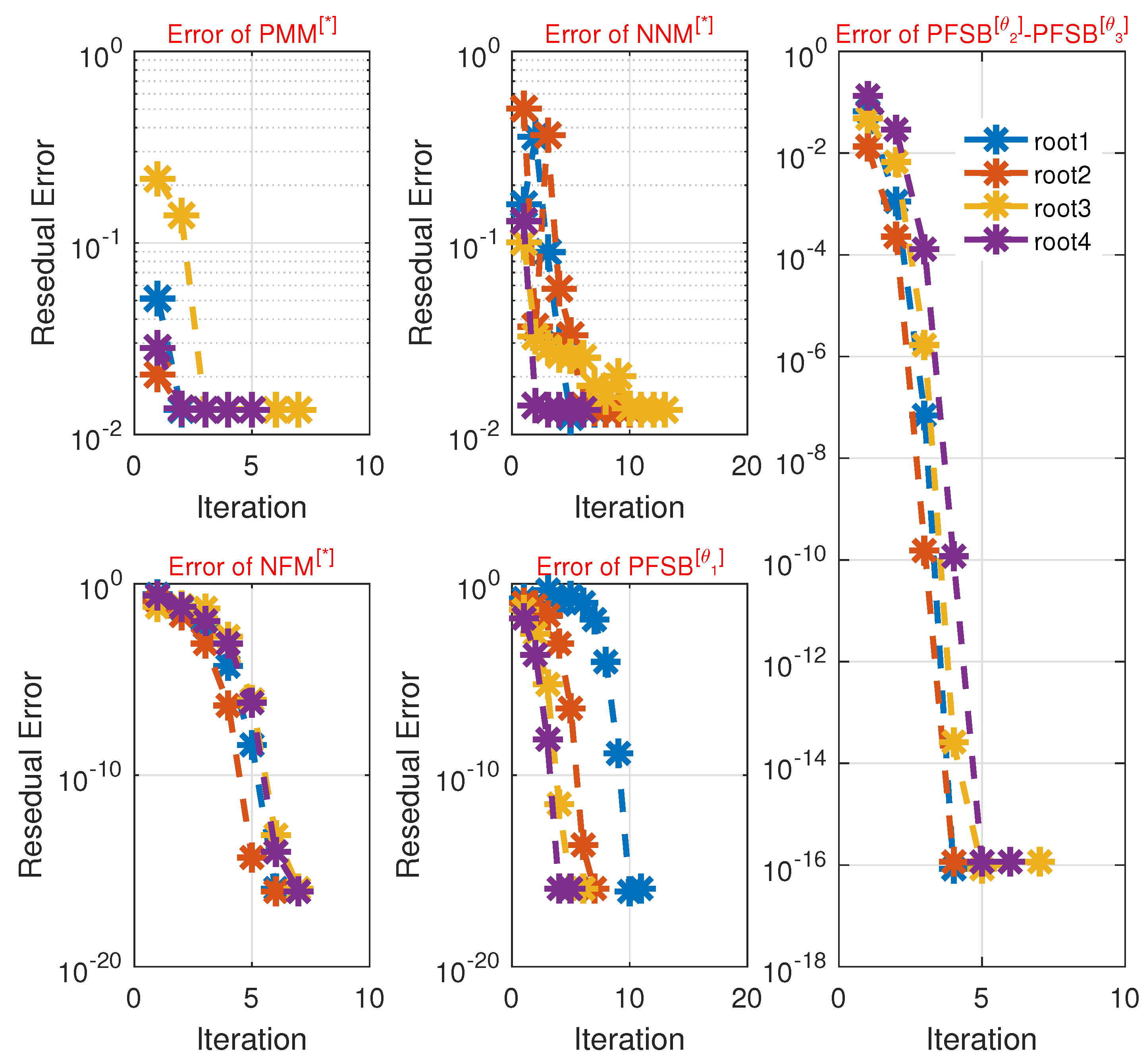
| Figure 8 illustrates the technique’s enhanced convergence for when compared to existing techniques. | For general problems, we use . For ill-conditioned or stiff eigenvalue problems, we used for improved robustness. |
| Scheme | ||||||
|---|---|---|---|---|---|---|
| Iterations | 26 | 27 | 30 | 28 | 20 | 21 |
| Percentage Convergence | 37.546% | 26.654% | 45.771% | 65.432% | 55.004% | 67.987% |
| Method | ||||
|---|---|---|---|---|
| Scheme | ||||||
|---|---|---|---|---|---|---|
| C-Time (s) | 5.7776 | 6.8865 | 6.7555 | 2.3646 | 3.6454 | 2.2436 |
| Memory Usage (%) | 77.436 | 68.998 | 51.565 | 48.002 | 47.070 | 39.986 |
| Scheme | Max-Err | Max-It | Per-Divergence (%) | |
|---|---|---|---|---|
| 22 | 44.0 | 58.1265 | ||
| 21 | 48.0 | 55.0003 | ||
| 20 | 46.0 | 47.9860 | ||
| 16 | 26.0 | 48.5555 | ||
| 11 | 36.0 | 33.0045 | ||
| 8 | 35.0 | 23.1100 |
| Scheme | |||||
|---|---|---|---|---|---|
| CPU−time | |||||
| Max-Err |
Disclaimer/Publisher’s Note: The statements, opinions and data contained in all publications are solely those of the individual author(s) and contributor(s) and not of MDPI and/or the editor(s). MDPI and/or the editor(s) disclaim responsibility for any injury to people or property resulting from any ideas, methods, instructions or products referred to in the content. |
© 2025 by the authors. Licensee MDPI, Basel, Switzerland. This article is an open access article distributed under the terms and conditions of the Creative Commons Attribution (CC BY) license (https://creativecommons.org/licenses/by/4.0/).
Share and Cite
Shams, M.; Carpentieri, B. A High-Order Fractional Parallel Scheme for Efficient Eigenvalue Computation. Fractal Fract. 2025, 9, 313. https://doi.org/10.3390/fractalfract9050313
Shams M, Carpentieri B. A High-Order Fractional Parallel Scheme for Efficient Eigenvalue Computation. Fractal and Fractional. 2025; 9(5):313. https://doi.org/10.3390/fractalfract9050313
Chicago/Turabian StyleShams, Mudassir, and Bruno Carpentieri. 2025. "A High-Order Fractional Parallel Scheme for Efficient Eigenvalue Computation" Fractal and Fractional 9, no. 5: 313. https://doi.org/10.3390/fractalfract9050313
APA StyleShams, M., & Carpentieri, B. (2025). A High-Order Fractional Parallel Scheme for Efficient Eigenvalue Computation. Fractal and Fractional, 9(5), 313. https://doi.org/10.3390/fractalfract9050313