Strong Convergence of a Modified Euler—Maruyama Method for Mixed Stochastic Fractional Integro—Differential Equations with Local Lipschitz Coefficients

Abstract

This paper presents a modified Euler—Maruyama (EM) method for mixed stochastic fractional integro—differential equations (mSFIEs) with Caputo—type fractional derivatives whose coefficients satisfy local Lipschitz and linear growth conditions. First, we transform the mSFIEs into an equivalent mixed stochastic Volterra integral equations (mSVIEs) using a fractional calculus technique. Then, we establish the well—posedness of the analytical solutions of the mSVIEs. After that, a modified EM scheme is formulated to approximate the numerical solutions of the mSVIEs, and its strong convergence is proven based on local Lipschitz and linear growth conditions. Furthermore, we derive the modified EM scheme under the same conditions in the $L^2$ sense, which is consistent with the strong convergence result of the corresponding EM scheme. Notably, the strong convergence order under local Lipschitz conditions is inherently lower than the corresponding order under global Lipschitz conditions. Finally, numerical experiments are presented to demonstrate that our approach not only circumvents the restrictive integrability conditions imposed by singular kernels, but also achieves a rigorous convergence order in the $L^2$ sense.

1. Introduction

Mixed stochastic fractional integro—differential equations (mSFIEs) are essential tools for understanding certain system properties that cannot be captured with a deterministic framework; for example, such equations can capture the long—memory effects arising from macroeconomic factors or systemic trends [1,2,3].

Many numerical methods have been developed for SFIEs, such as the EM method [4,5,6,7], stopped Euler—Maruyama method [3,8], truncated Euler—Maruyama method [9,10,11], Milstein method [12,13]), $\theta -$Maruyama method [14,15], explicit Euler method [16], and implicit Euler method [17]. In particular, the authors of [3] considered a class of mixed SDEs driven by both Brownian motion and fractional Brownian motion (fBm) with the Hurst parameter $H\in (1/2,1)$, and they obtained the convergence rate $\sqrt{\delta }$ (the diameter of partition) using a modified Euler method. In [4], the authors proved strong first—order superconvergence for linear SVIEs with convolution kernels when the kernel of the diffusion term becomes 0. In [5], nonlinear SFIEs were considered under non—Lipschitz conditions, and the EM solutions of SFIDEs shared strong first—order convergence. The authors of [7] introduced the initial value problem of Caputo—tempered SFIEs and proved the well—posedness of its solution, and the strong convergence order of the derived EM method was reported to be $\alpha -{\displaystyle \frac{1}{2}}$, with the fractional derivative’s order $\alpha \in (1/2,1)$. Additionally, a fast EM method based on the sum—of—exponentials approximation was developed. However, most SDE models in real—world applications do not satisfy the global Lipschitz condition in the analysis of numerical solutions, especially Caputo—type fractional SDEs [5,18,19], where the local Lipschitz condition alone is insufficient to guarantee the existence of a global solution [12,20,21]. In [21], the authors found that, under linear growth conditions (Khasminskii—type conditions), both the exact and numerical solutions obtained via the EM or stochastic theta method satisfy the moment—boundedness condition, thereby establishing the strong convergence of the numerical solutions to the exact solution under local Lipschitz and linear growth conditions [9,10,11]. As the classical explicit EM method has a simple structure, is not time—consuming, and has an acceptable convergence rate under the global Lipschitz condition, it has attracted significant attention [16,17,22].

Additionally, research on the above numerical methods for SFIEs or SVIEs has concentrated on convergence under global Lipschitz and linear growth conditions, but the numerical stability properties of SFIEs or Hölder continuous kernels under local Lipschitz and linear growth conditions are rarely discussed. Specifically, no results have been reported on the mean—square stability of the analytical solutions of mSFIEs with singular kernels. Based on the Caputo—type fractional SDE, we consider the following mSFIE in It$\hat{\mathrm{o}}$’s sense:

$$\begin{array}{cc}\hfill D^{\alpha }y\left(t\right)& =k_0(t,y\left(t\right))+k_1(t,s,y\left(s\right)){\displaystyle \frac{\mathrm{d}s}{\mathrm{d}t}}+k_2(t,s,y\left(s\right)){\displaystyle \frac{\mathrm{d}{W}_t}{\mathrm{d}t}}+k_3(t,s,y\left(s\right)){\displaystyle \frac{\mathrm{d}{W}_t^H}{\mathrm{d}t}},\hfill \\ \hfill t& \in \mathcal{T},y\left(0\right)=y_0,\hfill \end{array}$$

(1)

where $D^{\alpha }$ represents the Caputo—type fractional derivative of order $\alpha \in (1/2,1)$ on $\mathcal{T}\triangleq [0,T]$, $k_0\in L^1(\mathcal{T}\times {\mathbb{R}}^d;{\mathbb{R}}^d)$, $k_1\in L^1(\{(t,s):0\le s\le t\le T\}\times {\mathbb{R}}^d;{\mathbb{R}}^d)$, $k_2\in L^2(\{(t,s):0\le s\le t\le T\}\times {\mathbb{R}}^d;{\mathbb{R}}^{d\times r})$, and $k_3\in L^2(\{(t,s):0\le s\le t\le T\}\times {\mathbb{R}}^d;{\mathbb{R}}^{d\times r})$. $W_t$ is defined as an $r-$dimensional standard Brownian motion on the complete probability space $(\Omega ,\mathcal{F},\mathbb{P})$ with an algebra filtration $\{{\mathcal{F}}_t,t\ge 0\}$, where ${\mathcal{F}}_t$ is right—continuous, and ${\mathcal{F}}_0$ contains all $\mathbb{P}$-null sets. $y_0$ is an ${\mathcal{F}}_0-$measurable ${\mathbb{R}}^d-$valued random variable, which is defined on the same probability space and satisfies $\mathbb{E}|y_0{|}^2<\infty$. $W_t^H$ is an fBm defined on $(\Omega ,\mathcal{F},\mathbb{P})$. As observed above, mSFIE (1) includes the Riemann—Liouville fractional integral operator and the fBm process. It becomes more complex to compare classical SDEs containing Brownian motion and fBm. Two major difficulties arise when investigating stochastic equations driven by $W_t^H$; namely, the presence of correlated increments and the absence of the martingale property, which compromises the validity of the classical convergence theorem [12] in numerical analysis. In addition, it is challenging to determine the stability properties of analytical and numerical solutions, necessitating further in—depth research.

To the best of our knowledge, few studies have investigated the convergence rate of the numerical solutions of mSFIE (1) under local Lipschitz and linear growth conditions. To overcome the above difficulties and obtain the strong convergence rates in additive noise cases when $H\in (1/2,1)$, we first loosen the assumption of the global Lipschitz condition to the local Lipschitz condition and proceed to prove the well—posedness, and then we study the strong convergence order of the numerical method. We first transform the mSFIEs into the equivalent mSVIEs using a fractional calculus technique, and then we present the well—posedness of the analytical solutions of the mSVIEs. After that, a modified EM method is devised to approximate the numerical solutions of mSVIEs, and its strong convergence is obtained under local Lipschitz and linear growth conditions. Furthermore, we derive the modified EM scheme under the same conditions in the $L^2$ sense, which is consistent with the strong convergence result of the corresponding EM scheme. Notably, the strong convergence order under local Lipschitz conditions is inherently lower than the corresponding order under global Lipschitz conditions. Finally, numerical experiments are presented to demonstrate that our approach not only circumvents the restrictive integrability conditions imposed by singular kernels, but also achieves a rigorous convergence order in the $L^2$ sense.

The structure of this paper is as follows. In Section 2, some basic notations, preliminary facts on stochastic integrals for fBm, and some special functions are given, and some mild hypotheses are constructed. In Section 3, we transform the mSFIE into an equivalent mSVIE using a fractional calculus technique and Malliavin calculus. In Section 4, we employ a modified EM approximation to study the well—posedness of the solution to the mSVIE. In Section 5, we derive the strong convergence order of the modified EM method under local Lipschitz and linear growth conditions in the mean—square sense. Numerical experiments are presented in Section 6. Finally, we end with a brief conclusion in Section 7.

2. Preliminaries

In this paper, $\mathbb{E}$ denotes the expectation corresponding to $\mathbb{P}$. Let $|·|$ be the Euclidean norm $\left|x\right|=\sqrt{{\sum }_{i=1}^d{x}_i^2}$ on ${\mathbb{R}}^d$ and the trace norm $\parallel ·\parallel$ on ${\mathbb{R}}^{d\times r}$. We define matrix A, and then $\parallel A\parallel =\sqrt{\mathtt{trace}\left(A^{T}A\right)}$ for $A\in {\mathbb{R}}^{d\times r}$. Consider a complete probability space $(\Omega ,\mathcal{F},\mathbb{P})$ with a filtration ${\left\{{\mathcal{F}}_t\right\}}_{t\ge 0}$ that satisfies common assumptions. For the real numbers a, b, and c, we write $a\wedge b\wedge c:=min\{a,b,c\}$ and $a\vee b\vee c:=max\{a,b,c\}$. The following notations and preliminaries are provided in [23,24].

Definition 1 

([23,24]). Let $a,b\in \mathbb{R}$ and $a<b$, and let $f\in L^1\left([a,b]\right)$ and $0<\alpha <1$. The $\alpha -$order left—sided fractional Riemann—Liouville integral of f on $[a,b]$ is defined as

$$\begin{array}{c}\hfill I_{a+}^{\alpha }{f}_t={\displaystyle \frac{1}{\Gamma \left(\alpha \right)}}{\int }_a^t{(t-s)}^{\alpha -1}{f}_s\mathrm{d}s,\end{array}$$

and the $\alpha -$order right—sided fractional Riemann—Liouville integral of f on $[a,b]$ is defined as

$$\begin{array}{c}\hfill I_{b-}^{\alpha }{f}_t={\displaystyle \frac{exp\{-i\pi \alpha \}}{\Gamma \left(\alpha \right)}}{\int }_t^b{(s-t)}^{\alpha -1}{f}_s\mathrm{d}s,\end{array}$$

where $\Gamma (·)$ denotes the Gamma function.

Consider two continuous functions $f,g\in L^1\left([a,b]\right)$ and $0<\alpha <1$. For almost all $t\in (a,b)$, we define the following fractional derivatives:

$$\begin{array}{c}\hfill \begin{array}{cc}& \left(D_{a+}^{\alpha }{f}_{a+}\right)\left(t\right)={\displaystyle \frac{1}{\Gamma (1-\alpha )}}\left[{\displaystyle \frac{f_t}{{(t-a)}^{\alpha }}}+\alpha {\int }_a^t{\displaystyle \frac{f_t-f_s}{{(t-s)}^{\alpha +1}}}\mathrm{d}s\right]{\mathbf{1}}_{(a,b)}\left(t\right),\hfill \\ & \left(D_{b-}^{1-\alpha }{g}_{b-}\right)\left(t\right)={\displaystyle \frac{exp\{-i\pi \alpha \}}{\Gamma \left(\alpha \right)}}\left[{\displaystyle \frac{g_t}{{(b-t)}^{1-\alpha }}}+(1-\alpha ){\int }_t^b{\displaystyle \frac{g_t-g_{\tau }}{{(\tau -t)}^{2-\alpha }}}\mathrm{d}\tau \right]{\mathbf{1}}_{(a,b)}\left(t\right).\hfill \end{array}\end{array}$$

Assume that $D_{a+}^{\alpha }{f}_{a+}\in L^1\left([a,b]\right)$ and $D_{b-}^{1-\alpha }g\in L^p\left([a,b]\right)$, where $f_{a+}\left(t\right)=f_t-f_a$ and $g_{b-}\left(t\right)=g_t-g_b$. Under these assumptions, the generalized (fractional) Lebesgue—Stieltjes integral ${\int }_a^b{f}_t\mathrm{d}{g}_t$ is defined as

$$\begin{array}{c}\hfill {\int }_a^b{f}_t\mathrm{d}{g}_t=exp\{-i\pi \alpha \}{\int }_a^b\left(D_{a+}^{\alpha }{f}_{a+}\right)\left(t\right)·\left(D_{b-}^{1-\alpha }{g}_{b-}\right)\left(t\right)\mathrm{d}t,\end{array}$$

(2)

Note that, for all $0<\epsilon <H$, fBm $W_t^H$ has the ($H-\epsilon$) Hölder regularity of continuous paths. Then, for $f\in L^{\epsilon }\left([a,b]\right)$ and $1-H<\alpha <\epsilon <1/2$, the explicit expression in (2) becomes

$$\begin{array}{c}\hfill {\int }_a^b{f}_t\mathrm{d}{W}_t^H=exp\{-i\pi \alpha \}{\int }_a^b\left(D_{a+}^{\alpha }{f}_{a+}\right)\left(t\right)·\left(D_{b-}^{1-\alpha }{W}_{b-}^H\right)\left(t\right)\mathrm{d}t,\end{array}$$

(3)

where $W_{b-}^H\left(t\right)=W_b^H-W_t^H$.

Definition 2. 

We define the following norms for $\alpha \in (1-H,1/2)$:

$$\begin{array}{c}\hfill {\parallel f\parallel }_{0,\alpha ;t}=\underset{0\le u<v<T}{sup}\left({\displaystyle \frac{|f_t-f_s|}{{(t-s)}^{1-\alpha }}}+{\int }_u^v{\displaystyle \frac{|f_u-f_z|}{{(z-u)}^{2-\alpha }}}\mathrm{d}z\right),\end{array}$$

$$\begin{array}{cc}\hfill & {\parallel f\parallel }_{2,\alpha ;t}^2={\int }_0^t{\parallel f\parallel }_{\alpha ;s}^{2}g(t,s)\mathrm{d}s,\hfill \\ \hfill & {\parallel f\parallel }_{\infty ,\alpha ;t}=\underset{s\in [0,t]}{sup}{\parallel f\parallel }_{\alpha ;s},\hfill \end{array}$$

where $g(t,s)=s^{-\alpha }+{(t-s)}^{-\alpha -1/2}$, and

$$\begin{array}{c}\hfill \begin{array}{cc}& {\parallel f\parallel }_{\alpha ;t}=\left|f_t\right|+{\int }_0^t{\displaystyle \frac{|f_t-f_s|}{{(t-s)}^{1+\alpha }}}\mathrm{d}s,\hfill \\ & {\parallel f\parallel }_{\infty ,0,T;\alpha }=\underset{0\le t\le T}{sup}\left|f_t\right|+\underset{0\le s<t\le T}{sup}{\displaystyle \frac{|f_t-f_s|}{{(t-s)}^{\alpha }}}.\hfill \end{array}\end{array}$$

Next, we formulate some necessary mild hypotheses, which will be used in the next section.

Assumption 1. 

There exists a constant ${\mathcal{L}}_1>0$ that, for any $t_1,t_2,s\in \mathcal{T}$, $y\in {\mathbb{R}}^d$, such that $k_i$$(i=1,2,3)$, satisfies the following condition:

$$\begin{array}{c}\hfill \begin{array}{cc}\hfill |k_1(t_1,s,y)-k_1(t_2,s,y)|& +|k_2(t_1,s,y)-k_2(t_2,s,y)|\hfill \\ & +|k_3(t_1,s,y)-k_3(t_2,s,y)|\le {\mathcal{L}}_1(1+|y\left|\right)·|t_2-t_1|.\hfill \end{array}\end{array}$$

Assumption 2. 

There exists a constant ${\mathcal{L}}_2>0$ that, for any $t,s_1,s_2\in \mathcal{T}$, $y\in {\mathbb{R}}^d$, such that $k_i(t,s,y\left(s\right))$$(i=1,2,3)$, satisfies the following condition:

$$\begin{array}{c}\hfill \begin{array}{cc}\hfill |k_0(s_1,y)-k_0(s_2,y)|& \vee |k_1(t,s_1,y)-k_1(t,s_2,y)|\vee |k_2(t,s_1,y)-k_2(t,s_2,y)|\hfill \\ & \vee |k_3(t,s_1,y)-k_3(t,s_2,y)|\le {\mathcal{L}}_2(1+|y\left|\right)·|s_2-s_1|.\hfill \end{array}\end{array}$$

Assumption 3. 

There exists a constant ${\mathcal{L}}_m>0$$(m\ge 1)$ that is dependent on m and, for any $s,t\in \mathcal{T}$, $y_1,y_2\in {\mathbb{R}}^d$ and $|y_1|\vee |y_2|\le m$, such that $k_i$$(i=1,2,3)$, satisfies the following condition:

$$\begin{array}{c}\hfill \begin{array}{cc}\hfill |k_0(s,y_1)-k_0(s,y_2)|& \vee |k_1(t,s,y_1)-k_1(t,s,y_2)|\vee |k_2(t,s,y_1)-k_2(t,s,y_2)|\hfill \\ & \vee |k_3(t,s,y_1)-k_3(t,s,y_2)|\le {\mathcal{L}}_m(1+|y\left|\right)·|y_2-y_1|.\hfill \end{array}\end{array}$$

Assumption 4. 

There exists a constant ${\mathcal{L}}_4>0$ that, for any $s,t\in \mathcal{T}$, $y\in {\mathbb{R}}^d$, such that $k_i$$(i=1,2,3)$, satisfies the following linear growth condition:

$$\begin{array}{c}\hfill |k_0(s,y)|\vee |k_1(t,s,y)|\vee |k_2(t,s,y)|\vee |k_3(t,s,y)|\le {\mathcal{L}}_4(1+|y\left|\right).\end{array}$$

Remark 1. 

In Assumption 3, we point out that this local Lipschitz condition is significantly weaker than the following global Lipschitz condition; that is, there exists a constant $\mathcal{L}>0$ that, for any $s,t\in \mathcal{T}$, $y_1,y_2\in {\mathbb{R}}^d$, such that $k_i$$(i=1,2,3)$, satisfies the following condition:

$$\begin{array}{c}\hfill \begin{array}{cc}\hfill |k_0(s,y_1)-k_0(s,y_2)|& \vee |k_1(t,s,y_1)-k_1(t,s,y_2)|\vee |k_2(t,s,y_1)-k_2(t,s,y_2)|\hfill \\ & \vee |k_3(t,s,y_1)-k_3(t,s,y_2)|\le \mathcal{L}·|y_2-y_1|.\hfill \end{array}\end{array}$$

3. An Equivalent mSVIE

In this section, an equivalent mSVIE of mSFIE (1) is formulated for the deterministic fractional integral equation see [25] Section 2.2.2. page 119, [26] Section 3.1.3. page 204, and the integral Equation (2.14) of [27]. The integral equation form of mSFIE (1) can be rigorously defined to form the following mSVIE:

$$\begin{array}{cc}\hfill y\left(t\right)=y_0& +{\displaystyle \frac{1}{\Gamma \left(\alpha \right)}}{\int }_0^t{(t-\tau )}^{\alpha -1}{k}_0(\tau ,y\left(\tau \right))\mathrm{d}\tau \hfill \\ & +{\displaystyle \frac{1}{\Gamma \left(\alpha \right)}}{\int }_0^t{(t-\tau )}^{\alpha -1}\left[{\int }_0^{\tau }{k}_1(\tau ,s,y\left(s\right))\mathrm{d}s\right]\mathrm{d}\tau \hfill \\ & +{\displaystyle \frac{1}{\Gamma \left(\alpha \right)}}{\int }_0^t{(t-\tau )}^{\alpha -1}\left[{\int }_0^{\tau }{k}_2(\tau ,s,y\left(s\right))\mathrm{d}{W}_s\right]\mathrm{d}\tau \hfill \\ & +{\displaystyle \frac{1}{\Gamma \left(\alpha \right)}}{\int }_0^t{(t-\tau )}^{\alpha -1}\left[{\int }_0^{\tau }{k}_3(\tau ,s,y\left(s\right))\mathrm{d}{W}_s^H\right]\mathrm{d}\tau .\hfill \end{array}$$

(4)

Similar to the solution definition of the stochastic integral equation in [20] (Section 2.2. page 48, Definition 2.1), the solution of mSFIE (1) can be defined as follows.

Definition 3. 

Let $\left\{y\right(t):t\in \mathcal{T}\}$ be an ${\mathbb{R}}^d-$valued stochastic process if it satisfies the following conditions:

(1) $\left\{y\right(t\left)\right\}$ is ${\mathcal{F}}_t-$adapted and continuous;

(2) $k_0\in L^1(\mathcal{T}\times {\mathbb{R}}^d;{\mathbb{R}}^d)$, $k_1\in L^1(\{(t,s):0\le s\le t\le T\}\times {\mathbb{R}}^d;{\mathbb{R}}^d)$, $k_2\in L^2(\{(t,s):0\le s\le t\le T\}\times {\mathbb{R}}^d;{\mathbb{R}}^{d\times r})$, and $k_3\in L^2(\{(t,s):0\le s\le t\le T\}\times {\mathbb{R}}^d;{\mathbb{R}}^{d\times r})$;

(3) mSVIE (4) holds for every $t\in \mathcal{T}$ with probability 1.

A solution $\left\{y\right(t\left)\right\}$ is determined to be unique if any other solution $\left\{\tilde{y}\left(t\right)\right\}$ is indistinguishable from $\left\{y\right(t\left)\right\}$, such that

$$\begin{array}{c}\hfill \mathbb{P}\{y\left(t\right)=\tilde{y}\left(t\right)forallt\in \mathcal{T}\}=1.\end{array}$$

Under Assumption 1, we can use the stochastic Fubini theorem (ref. [2] Theorem 1.13.1. page 57) for mSVIE (4); then,

$$\begin{array}{cc}\hfill y\left(t\right)=y_0& +{\displaystyle \frac{1}{\Gamma \left(\alpha \right)}}{\int }_0^t{(t-\tau )}^{\alpha -1}{k}_0(\tau ,y\left(\tau \right))\mathrm{d}\tau \hfill \\ & +{\displaystyle \frac{1}{\Gamma \left(\alpha \right)}}{\int }_0^t{(t-\tau )}^{\alpha -1}\left[{\int }_0^{\tau }{k}_1(\tau ,s,y\left(s\right))\mathrm{d}\tau \right]\mathrm{d}s\hfill \\ & +{\displaystyle \frac{1}{\Gamma \left(\alpha \right)}}{\int }_0^t{(t-\tau )}^{\alpha -1}\left[{\int }_0^{\tau }{k}_2(\tau ,s,y\left(s\right))\mathrm{d}\tau \right]\mathrm{d}{W}_s\hfill \\ & +{\displaystyle \frac{1}{\Gamma \left(\alpha \right)}}{\int }_0^t{(t-\tau )}^{\alpha -1}\left[{\int }_0^{\tau }{k}_3(\tau ,s,y\left(s\right))\mathrm{d}\tau \right]\mathrm{d}{W}_s^H.\hfill \end{array}$$

(5)

We let

$$\begin{array}{c}\hfill \left.\begin{array}{cc}& K_0(t,s,y\left(s\right))={\displaystyle \frac{1}{\Gamma \left(\alpha \right)}}{\int }_0^t{(t-\tau )}^{\alpha -1}·k_0(s,y\left(s\right))\mathrm{d}\tau ,\hfill \\ & K_1(t,s,y\left(s\right))={\displaystyle \frac{1}{\Gamma \left(\alpha \right)}}{\int }_0^t{(t-\tau )}^{\alpha -1}·k_1(\tau ,s,y\left(s\right))\mathrm{d}\tau ,\hfill \\ & K_2(t,s,y\left(s\right))={\displaystyle \frac{1}{\Gamma \left(\alpha \right)}}{\int }_0^t{(t-\tau )}^{\alpha -1}·k_2(\tau ,s,y\left(s\right))\mathrm{d}\tau ,\hfill \\ & K_3(t,s,y\left(s\right))={\displaystyle \frac{1}{\Gamma \left(\alpha \right)}}{\int }_0^t{(t-\tau )}^{\alpha -1}·k_3(\tau ,s,y\left(s\right))\mathrm{d}\tau ,\hfill \end{array}\right\}\end{array}$$

(6)

and then mSVIE (5) is equivalent to the following mSVIE:

$$\begin{array}{cc}\hfill y\left(t\right)=y_0+{\int }_0^t{K}_0(t,s,y\left(s\right))\mathrm{d}s+{\int }_0^t{K}_1(t,s,y\left(s\right))\mathrm{d}s& +{\int }_0^t{K}_2(t,s,y\left(s\right))\mathrm{d}{W}_s\hfill \\ & +{\int }_0^t{K}_3(t,s,y\left(s\right))\mathrm{d}{W}_s^H.\hfill \end{array}$$

(7)

For technical reasons, we need the following auxiliary lemmas.

Lemma 1. 

Let $g:\mathcal{T}\to {\mathbb{R}}^d$ be an $\epsilon -$Hölder continuous function. We define $g^{\mathbf{c}}\left(t\right)={\displaystyle \frac{1}{\mathbf{c}}}{\int }_{0\vee t-\mathbf{c}}^{t}g\left(\tau \right)\mathrm{d}\tau$ for $\mathbf{c}>0$ and $t_1,t_2,s_1,s_2\in \mathcal{T}$. Then, for $\alpha \in (1-\epsilon ,1)$, there exists a constant $C^{\ast }>0$ such that

$$\parallel g\left(t\right)-g^{\mathbf{c}}{\left(t\right)\parallel }_{p,0,T;\alpha }\le C^{\ast }{\mathcal{L}}_{\epsilon }\left(g\right){\mathbf{c}}^{\epsilon +\alpha -1},t\in \mathcal{T},$$

where

$${\mathcal{L}}_{\epsilon }\left(g\right)=\underset{0\le |s_1-s_2|<|t_1-t_2|\le T}{sup}{\displaystyle \frac{\left|g\right(|t_1-t_2\left|\right)-g\left(\right|s_1-s_2\left|\right)|}{\left(\right|t_1-t_2|-|s_1-s_2{\left|\right)}^{\epsilon }}}$$

is the ε-Hölder constant of $g\left(t\right)$.

The proof can be seen in Appendix A.

Lemma 2. 

Under Assumptions 1–4, for any $\alpha \in (1-H,{\displaystyle \frac{1}{2}})$, mSVIE (7) has a unique solution $y\left(t\right)$ such that $\{y\left(t\right),t\in \mathcal{T}\}\in L_0^{\alpha ,p}(\mathcal{T},{\mathbb{R}}^d)$$a.s.$ Furthermore, for any $0<\eta <{\displaystyle \frac{1}{2}}$ and $s\le t\in \mathcal{T}$, there exists a constant $C>0$ such that

$$\parallel y\left(t\right)-y^{\mathit{c}}\left(t\right)-y\left(s\right)+y^{\mathit{c}}{\left(s\right)\parallel }_{p,0,T;\alpha }\le C{\mathcal{L}}_{2\alpha +({\displaystyle \frac{1}{2}}-\eta )}\left(y\right){\mathit{c}}^{2\alpha +({\displaystyle \frac{1}{2}}-\eta )},$$

(8)

where

$${\mathcal{L}}_{2\alpha +({\displaystyle \frac{1}{2}}-\eta )}\left(y\right)=\underset{0\le s<t\le T}{sup}{\displaystyle \frac{y\left(t\right)-y\left(s\right)}{{(t-s)}^{2\alpha +(\frac{1}{2}-\eta )}}}$$

is the $[2\alpha +({\displaystyle \frac{1}{2}}-\eta )]$-Hölder constant of $y\left(t\right)$.

The proof can be seen in Appendix B.

4. Existence and Uniqueness of Solution to mSVIE (7)

In this section, we employ a modified EM approximation with the aim of proving the existence, uniqueness, and stability of the solution to mSVIE (7).

4.1. A Modified EM Scheme

For every integer $N\ge 1$, we let ${\mathcal{T}}_N\triangleq \{t_n\triangleq {\displaystyle \frac{nT}{N}}=nh:n=0,1,\dots ,N\}$ be a given uniform mesh on $\mathcal{T}$. Then, we can define a stopping time ${\tau }_N=T\wedge {inf\{t:\parallel W\parallel }_{0,t}\ge N\}$ and a stopped process $W_t^N=W_{t\wedge {\tau }_N}$. The solution of mSVIE (7) is denoted by $y^N$, with W replaced by $W^N$. For $t=t_n$, mSVIE (7) becomes

$$\begin{array}{cc}\hfill y\left(t_n\right)& =y_0+{\int }_0^{t_n}{K}_0(t_n,s,y\left(s\right))\mathrm{d}s+{\int }_0^{t_n}{K}_1(t_n,s,y\left(s\right))\mathrm{d}s\hfill \\ & +{\int }_0^{t_n}{K}_2(t_n,s,y\left(s\right))\mathrm{d}{W}_s+{\int }_0^{t_n}{K}_3(t_n,s,y\left(s\right))\mathrm{d}{W}_s^H\hfill \\ \hfill & =y_0+\sum _{i=0}^{n-1}{\int }_{t_i}^{t_{i+1}}{K}_0(t_n,s,y\left(s\right))\mathrm{d}s+\sum _{i=0}^{n-1}{\int }_{t_i}^{t_{i+1}}{K}_1(t_n,s,y\left(s\right))\mathrm{d}s\hfill \\ & +\sum _{i=0}^{n-1}{\int }_{t_i}^{t_{i+1}}{K}_2(t_n,s,y\left(s\right))\mathrm{d}{W}_s+\sum _{i=0}^{n-1}{\int }_{t_i}^{t_{i+1}}{K}_3(t_n,s,y\left(s\right))\mathrm{d}{W}_s^H\hfill \\ & \approx y_0+\sum _{i=0}^{n-1}{\int }_{t_i}^{t_{i+1}}{K}_0(t_n,s,y\left(t_i\right))\mathrm{d}s+\sum _{i=0}^{n-1}{\int }_{t_i}^{t_{i+1}}{K}_1(t_n,s,y\left(t_i\right))\mathrm{d}s\hfill \\ & +\sum _{i=0}^{n-1}{\int }_{t_i}^{t_{i+1}}{K}_2(t_n,s,y\left(t_i\right))\mathrm{d}{W}_s+\sum _{i=0}^{n-1}{\int }_{t_i}^{t_{i+1}}{K}_3(t_n,s,y\left(t_i\right))\mathrm{d}{W}_s^H,\hfill \end{array}$$

(9)

and

$$\begin{array}{cc}\hfill & y^N\left(t_n\right)\hfill \\ & =y_0^N+\sum _{i=0}^{n-1}{\int }_{t_i}^{t_{i+1}}{K}_0(t_n,s,y^N\left(t_i\right))\mathrm{d}s+\sum _{i=0}^{n-1}{\int }_{t_i}^{t_{i+1}}{K}_1(t_n,s,y^N\left(t_i\right))\mathrm{d}s\hfill \\ & +\sum _{i=0}^{n-1}{\int }_{t_i}^{t_{i+1}}{K}_2(t_n,s,y^N\left(t_i\right))\mathrm{d}{W}_s+\sum _{i=0}^{n-1}{\int }_{t_i}^{t_{i+1}}{K}_3(t_n,s,y^N\left(t_i\right))\mathrm{d}{W}_s^H,\hfill \end{array}$$

(10)

for $n=1,\dots ,N$ and $y^N\left(t_0\right)=y_0$. Let ${\widehat{y}}^N\left(t\right)={\sum }_{n=0}^N{y}^N\left(t_n\right){\mathcal{I}}_{[t_n,t_{n+1})}\left(t\right)$, $t\in \mathcal{T}$. Then, the modified EM scheme is as follows:

$$\begin{array}{cc}\hfill y^N\left(t\right)=y_0& +{\int }_0^t{K}_0(t,s,{\widehat{y}}^N\left(s\right))\mathrm{d}s+{\int }_0^t{K}_1(t,s,{\widehat{y}}^N\left(s\right))\mathrm{d}s\hfill \\ & +{\int }_0^t{K}_2(t,s,{\widehat{y}}^N\left(s\right))\mathrm{d}{W}_s+{\int }_0^t{K}_3(t,s,{\widehat{y}}^N\left(s\right))\mathrm{d}{W}_s^H.\hfill \end{array}$$

(11)

Obviously, the $[2\alpha +({\displaystyle \frac{1}{2}}-\eta )]-$Hölder continuous trajectory $y^N\left(t\right)$ satisfies $y^N\left(t_n\right)={\widehat{y}}^N\left(t_n\right)$ for $n=0,1,\dots ,N$.

4.2. Existence and Uniqueness

Lemma 3. 

Under Assumption 4, there exists a constant $C_N>0$ that is independent of N, and for any $p\ge 2/\theta$, $\theta \in (0,\alpha +H-{\displaystyle \frac{1}{2}})$, it satisfies

$$\begin{array}{c}\hfill \mathbb{E}[\parallel y^N{\left(t\right)\parallel }_{\infty ,0,T;\alpha }^p]\le C_{N}and\mathbb{E}[\parallel {\widehat{y}}^N\left(t\right){\parallel }_{\infty ,0,T;\alpha }^p]\le C_N,t\in \mathcal{T},\end{array}$$

where $N\ge 1$.

The proof can be seen in Appendix C.

Lemma 4. 

Under Assumptions 1 and 4, for any integer $p\ge 2/\theta$, $\theta \in (0,\alpha +H-{\displaystyle \frac{1}{2}})$, there exists a constant $C_N>0$ such that

$$\begin{array}{c}\hfill \mathbb{E}[\parallel y^N\left(t\right)-y^N\left(t^{\ast }\right){\parallel }_{\infty ,0,T;\alpha }^p]\le C_N{|t-t^{\ast }|}^{\alpha p},0\le t^{\ast }<t\le T,\end{array}$$

where $N\ge 1$.

The proof can be seen in Appendix D.

Theorem 1. 

Based on Assumption 1, Assumption 3, and Assumption 4, mSFIE (1) has a unique solution $y\left(t\right)$, and for any $p\ge 2/\theta$ (p is positive integer), $\theta \in (0,\alpha +H-{\displaystyle \frac{1}{2}})$, it satisfies

$$\mathbb{E}\left[\right|y\left(t\right){|}^p]<\infty ,t\in \mathcal{T}.$$

(12)

The proof is provided in Appendix E.

5. Strong Convergence Analysis of the Modified EM Approximation

Note that the numerical approximation provided by EM Scheme (11) in Section 4 will incur significant computational overhead with stochastic fractional integrals. In this section, we propose a modified version of Euler—Maruyama (EM) Scheme (11) that reduces computational complexity while preserving the desired strong convergence rates.

Given the setting with scheme (11), we design the modified version by using left—endpoint approximation [4]:

$$\begin{array}{cc}\hfill Y\left(t\right)=y_0& +{\int }_0^t{K}_0(t,\underline{s},\widehat{Y}\left(s\right))\mathrm{d}s+{\int }_0^t{K}_1(t,\underline{s},\widehat{Y}\left(s\right))\mathrm{d}s\hfill \\ & +{\int }_0^t{K}_2(t,\underline{s},\widehat{Y}\left(s\right))\mathrm{d}{W}_s+{\int }_0^t{K}_3(t,\underline{s},\widehat{Y}\left(s\right))\mathrm{d}{W}_s^H,\hfill \end{array}$$

(13)

where $\underline{s}=t_n$ for $s\in [t_n,t_{n+1})$, $\widehat{Y}\left(t\right)={\sum }_{n=0}^{N}Y\left(t_n\right){\mathcal{I}}_{[t_n,t_{n+1})}\left(t\right)$. Our modified EM method can be defined as follows:

$$\begin{array}{cc}\hfill Y_n:& =Y\left(t_n\right)\hfill \\ & =y_0+\sum _{j=0}^{n-1}{K}_0(t_n,t_j,Y_j)h+\sum _{j=0}^{n-1}{K}_1(t_n,t_j,Y_j)h+\sum _{j=0}^{n-1}{K}_2(t_n,t_j,Y_j)\Delta W_j\hfill \\ & +\sum _{j=0}^{n-1}{K}_3(t_n,t_j,Y_j)\Delta W_j^H,0\le n\le N,\hfill \\ \hfill Y_0& =y_0,\hfill \end{array}$$

(14)

where $\Delta W_j=W_{t_{j+1}}-W_{t_j}$ and $\Delta W_j^H=W_{t_{j+1}}^H-W_{t_j}^H$, $j=0,1,\cdots ,N-1$. Obviously, we only simulate $\Delta W_j$ and $\Delta W_j^H$ without computing stochastic integrals. Noticing that the discrete of the fBm increment in the interval $[j\Delta t,(j+1)\Delta t)$ can be using a binomial approach (see [28]), such as

$$\begin{array}{c}\hfill \Delta W_{j\Delta t}^H=\left\{\begin{array}{ccc}\sqrt{{(j+1)}^{2H}-j^{2H}}\Delta t^H,\hfill & \hfill \mathrm{with}\mathrm{probability}& 1/2\hfill \\ -\sqrt{{(j+1)}^{2H}-j^{2H}}\Delta t^H,\hfill & \hfill \mathrm{with}\mathrm{probability}& 1/2\hfill \end{array}\right.,\end{array}$$

and the fBm value on the interval $[0,i\Delta t]$ is computed as

$$W_{i\Delta t}^H=\sum _{j=0}^{i-1}\Delta W_{j\Delta t}^H,\mathrm{with}{W}_0^H=0\mathrm{and}i=1,\cdots ,n,$$

which effectively reduces the calculations.

5.1. The Mean—Square Convergence Theorem of the Modified EM Method (14)

To analyze the strong convergence of the modified EM method (14), the boundedness of the numerical solution can be established using the following lemma.

Lemma 5. 

Under the same conditions as Lemma 2, for any $t\in [t_n,t_{n+1}]$, $n=1,2,\cdots ,N-1$,

$$\parallel y(t-\underline{s})-y^{\mathit{c}}(t_n-\underline{s}){\parallel }_{p,0,T;\alpha }\le C{\mathcal{L}}_{2\alpha +({\displaystyle \frac{1}{2}}-\eta )}\left(y\right)h^{2\alpha +({\displaystyle \frac{1}{2}}-\eta )},$$

$$\parallel y(t-\underline{s})-y^{\mathit{c}}(t-s){\parallel }_{p,0,T;\alpha }\le C{\mathcal{L}}_{2\alpha +({\displaystyle \frac{1}{2}}-\eta )}\left(y\right)h^{2\alpha +({\displaystyle \frac{1}{2}}-\eta )},$$

where

$${\mathcal{L}}_{2\alpha +({\displaystyle \frac{1}{2}}-\eta )}\left(y\right)=\underset{\mathit{c}\ge 0}{sup}{\displaystyle \frac{y\left(\mathit{c}\right)}{{\mathit{c}}^{2\alpha +(\frac{1}{2}-\eta )}}}$$

is the $[2\alpha +({\displaystyle \frac{1}{2}}-\eta )]-$Hölder constant of $y\left(t\right)$.

The proof can be seen in Appendix F.

Lemma 6. 

Under Assumption 4, for any $t\in \mathcal{T}$, there exists a constant $C>0$, which is independent of h, for any integer $p\ge 2/\theta$, $\theta \in (0,\alpha +H-{\displaystyle \frac{1}{2}})$, such that

$$\begin{array}{c}\hfill {\mathbb{E}[\parallel Y\left(t\right)\parallel }_{\infty ,0,T;\alpha }^p]\le C,\mathbb{E}[\parallel \widehat{Y}\left(t\right){\parallel }_{\infty ,0,T;\alpha }^p]\le C.\end{array}$$

The proof is similar to that of Lemma 4.

Lemma 7. 

Under Assumptions 1 and 4, for any $t\in \mathcal{T}$, there exists a constant $C>0$ that, independent of h, satisfies

$$\begin{array}{c}\hfill \mathbb{E}[\parallel Y\left(t\right)-\widehat{Y}\left(t\right){\parallel }_{\infty ,0,T;\alpha }^2]\le C{h}^{2\alpha }.\end{array}$$

The proof can be seen in Appendix G.

Next, we study the mean-square convergence of the modified EM method (14) under Assumptions 3 and 4. More details of the properties of the local Lipschitz condition can be seen in Remark 2.1 of [29]. Notice that ${\mathcal{L}}_m$ is an increasing function depending on m, and we need to consider ${\mathcal{L}}_m\uparrow \infty$ as $m\to \infty$. Therefore, we let ${\Delta }_{\ast }>0$ be sufficiently small for a strictly positive decreasing function $\nu :(0,{\Delta }_{\ast }]\to (0,\infty )$ such that

$$\underset{h\to 0}{lim}\nu \left(h\right)=\infty ,\underset{h\to 0}{lim}{\mathcal{L}}_{\nu \left(h\right)}^2{h}^{2\mathcal{O}}=0,$$

(15)

where $\mathcal{O}$ denotes the order of the modified EM method under the global Lipschitz condition (Remark 1).

Theorem 2. 

Based on Assumptions 3 and 4, for the arbitrary constant $\zeta \in (0,2)$ and $p>{\displaystyle \frac{2}{\theta }}$, $\theta \in (0,\alpha +H-{\displaystyle \frac{1}{2}})$, we assume that there exists an h that satisfies

$$\begin{array}{c}\hfill \nu \left(h\right)\ge {\left[{\mathcal{L}}_{\nu \left(h\right)}^2{h}^{\mathcal{O}}\right]}^{-{\displaystyle \frac{p}{2(p-2)}}},where\mathcal{O}=\left\{\begin{array}{ccc}min\{2-\zeta ,2\alpha +1-2\theta \},\hfill & \hfill \alpha -\theta & =1/2,\hfill \\ min\{2,2\alpha +1-2\theta \},\hfill & \hfill \alpha -\theta & \ne 1/2\hfill \end{array}\right.\end{array}$$

and for any $h<{\Delta }_{\ast }$, there exists a constant $C>0$, which is independent of h. Then, the modified EM solution $Y\left(t\right)$ to mSVIE (14) converges to the exact solution $y\left(t\right)$, that is,

$${\mathbb{E}\left[\right|Y\left(t\right)-y\left(t\right)|}^2]\le C{\mathcal{L}}_{\nu \left(h\right)}^2{h}^{\mathcal{O}},forallt\in \mathcal{T}.$$

Proof. 

We define the error as

$$\mathbf{e}\left(t\right)=Y\left(t\right)-y\left(t\right)$$

and the stopping time as

$$\mathbf{t}=inf\{t\ge 0:|Y\left(t\right)|\ge m\}.$$

According to Theorem 1 and Lemma 7, for any $\delta >0$, we have

$$\begin{array}{c}\hfill \begin{array}{cc}& {\mathbb{E}[\parallel \mathbf{e}\left(t\right)\parallel }_{2,0,T;\alpha }^2{]=\mathbb{E}[\parallel \mathbf{e}\left(t\right)\parallel }_{{\mathbf{1}}_{\{\mathbf{t}>T,{\tau }_m^{\ast }>T\}}}^2{]+\mathbb{E}[\parallel \mathbf{e}\left(t\right)\parallel }_{{\mathbf{1}}_{\{[\mathbf{t}>T]\cup [{\tau }_m^{\ast }>T]\}}}^2]\hfill \\ & \le \mathbb{E}[\parallel \mathbf{e}(t\wedge \mathbf{t}\wedge {\tau }_m^{\ast }){\parallel }_{{\mathbf{1}}_{\{(\mathbf{t}\wedge {\tau }_m^{\ast })>T\}}}^2]+{\displaystyle \frac{2\delta \mathbb{E}\left[\right|\mathbf{e}\left(t\right){|}^p]}{p}}+{\displaystyle \frac{p-2}{p{\delta }^{2/(p-2)}}}\mathbb{P}\{[\mathbf{t}>T]\cup [{\tau }_m^{\ast }>T]\}\hfill \\ & \le \mathbb{E}[\parallel \mathbf{e}(t\wedge \mathbf{t}\wedge {\tau }_m^{\ast }){\parallel }_{{\mathbf{1}}_{\{(\mathbf{t}\wedge {\tau }_m^{\ast })>T\}}}^2]+{\displaystyle \frac{2\delta ·2^p\epsilon }{p}}+{\displaystyle \frac{p-2}{p{\delta }^{2/(p-2)}}}·{\displaystyle \frac{2\epsilon }{m^p}}\left(\mathrm{Young}’s \mathrm{inequality}\right)\hfill \\ & \le \mathbb{E}\left[\right|\mathbf{e}(t\wedge \mathbf{t}\wedge {\tau }_m^{\ast }){|}^2]+{\displaystyle \frac{\delta 2^{p+1}\epsilon }{p}}+{\displaystyle \frac{2(p-2)\epsilon }{p{\delta }^{2/(p-2)}{m}^p}},\hfill \end{array}\end{array}$$

(16)

where the constant $\epsilon >0$ is independent of $\delta$ and m. Furthermore, we can estimate $\mathbb{E}\left[\right|\mathbf{e}(t\wedge \mathbf{t}\wedge {\tau }_m^{\ast }){|}^2]$ in the last expression of inequality (16). With a Hölder—type inequality, we have

$$\begin{array}{c}\hfill \begin{array}{cc}& \mathbb{E}\left[\right|\mathbf{e}(t\wedge \mathbf{t}\wedge {\tau }_m^{\ast }){|}^2]\hfill \\ & \le 8\mathbb{E}\left\{\right|{\int }_0^{t\wedge \mathbf{t}\wedge {\tau }_m^{\ast }}[K_0(t\wedge \mathbf{t}\wedge {\tau }_m^{\ast },\underline{s},\widehat{Y}\left(s\right))-K_0(t\wedge \mathbf{t}\wedge {\tau }_m^{\ast },s,\widehat{Y}\left(s\right))]\mathrm{d}s{|}^2\hfill \\ & +|{\int }_0^{t\wedge \mathbf{t}\wedge {\tau }_m^{\ast }}[K_0(t\wedge \mathbf{t}\wedge {\tau }_m^{\ast },s,\widehat{Y}\left(s\right))-K_0(t\wedge \mathbf{t}\wedge {\tau }_m^{\ast },s,y\left(s\right))]\mathrm{d}s{|}^2\hfill \\ & +|{\int }_0^{t\wedge \mathbf{t}\wedge {\tau }_m^{\ast }}[K_1(t\wedge \mathbf{t}\wedge {\tau }_m^{\ast },\underline{s},\widehat{Y}\left(s\right))-K_1(t\wedge \mathbf{t}\wedge {\tau }_m^{\ast },s,\widehat{Y}\left(s\right))]\mathrm{d}s{|}^2\hfill \\ & +|{\int }_0^{t\wedge \mathbf{t}\wedge {\tau }_m^{\ast }}[K_1(t\wedge \mathbf{t}\wedge {\tau }_m^{\ast },s,\widehat{Y}\left(s\right))-K_1(t\wedge \mathbf{t}\wedge {\tau }_m^{\ast },s,y\left(s\right))]\mathrm{d}s{|}^2\hfill \\ & +|{\int }_0^{t\wedge \mathbf{t}\wedge {\tau }_m^{\ast }}[K_2(t\wedge \mathbf{t}\wedge {\tau }_m^{\ast },\underline{s},\widehat{Y}\left(s\right))\mathrm{d}{W}_s-K_2(t\wedge \mathbf{t}\wedge {\tau }_m^{\ast },s,\widehat{Y}\left(s\right)])\mathrm{d}{W}_s{|}^2\hfill \\ & +|{\int }_0^{t\wedge \mathbf{t}\wedge {\tau }_m^{\ast }}[K_2(t\wedge \mathbf{t}\wedge {\tau }_m^{\ast },s,\widehat{Y}\left(s\right))\mathrm{d}{W}_s-K_2(t\wedge \mathbf{t}\wedge {\tau }_m^{\ast },s,y\left(s\right)])\mathrm{d}{W}_s{|}^2\hfill \\ & +\left|{\int }_0^{t\wedge \mathbf{t}\wedge {\tau }_m^{\ast }}[K_3(t\wedge \mathbf{t}\wedge {\tau }_m^{\ast },\underline{s},\widehat{Y}\left(s\right))\mathrm{d}{W}_s^H-K_3(t\wedge \mathbf{t}\wedge {\tau }_m^{\ast },s,\widehat{Y}\left(s\right))]\mathrm{d}{W}_s^H{|}^2\right\}\hfill \\ & +\left|{\int }_0^{t\wedge \mathbf{t}\wedge {\tau }_m^{\ast }}[K_3(t\wedge \mathbf{t}\wedge {\tau }_m^{\ast },s,\widehat{Y}\left(s\right))\mathrm{d}{W}_s^H-K_3(t\wedge \mathbf{t}\wedge {\tau }_m^{\ast },s,y\left(s\right))]\mathrm{d}{W}_s^H{|}^2\right\}\hfill \\ & =:8\{{\mathfrak{K}}_1+{\mathfrak{K}}_2+{\mathfrak{K}}_3+{\mathfrak{K}}_4+{\mathfrak{K}}_5+{\mathfrak{K}}_6+{\mathfrak{K}}_7+{\mathfrak{K}}_8\}.\hfill \end{array}\end{array}$$

(17)

Using the Cauchy—Schwarz—type inequality and Itô isometry, under Assumption 1, Assumption 2, Assumption 4, and Lemmas 6–7, we have

$${\mathfrak{K}}_1+{\mathfrak{K}}_3+{\mathfrak{K}}_5+{\mathfrak{K}}_7\le C{h}^{2\alpha }.$$

(18)

With the Cauchy—Schwarz—type inequality and Itô isometry, under Assumption 3, combined with Theorem 1, we have

$$\begin{array}{cc}\hfill & {\mathfrak{K}}_2+{\mathfrak{K}}_4+{\mathfrak{K}}_6+{\mathfrak{K}}_8\hfill \\ & \le C{\mathcal{L}}_m^2{\int }_0^{t\wedge \mathbf{t}\wedge {\tau }_m^{\ast }}{[(t\wedge \mathbf{t}\wedge {\tau }_m^{\ast })-s]}^{\alpha -1}\mathbb{E}\left[\right|Y\left(s\right)-\widehat{Y}\left(s\right){|}^2+|\mathbf{e}(s\wedge \mathbf{t}\wedge {\tau }_m^{\ast }){|}^2]\mathrm{d}s.\hfill \end{array}$$

(19)

Applying Lemma 7 and the weakly singular Gronwall—type inequality (ref. [30], Theorem 3.3.1. page 349), we have

$$\mathbb{E}\left[\right|\mathbf{e}(t\wedge \mathbf{t}\wedge {\tau }_m^{\ast }){|}^2]\le \left\{\begin{array}{ccc}{C}_m{h}^{min\{2-\zeta ,2\alpha +1-2\theta \}},\hfill & \hfill \alpha -\theta & =1/2,\hfill \\ C_m{h}^{min\{2,2\alpha +1-2\theta \}},\hfill & \hfill \alpha -\theta & \ne 1/2\hfill \end{array}\right..$$

Note that the constant $C_m$ depends on m, and it is independent of h and $\delta$. Then, (16) becomes

$$\begin{array}{c}\hfill \begin{array}{c}\hfill {\mathbb{E}[\parallel \mathbf{e}\left(t\right)\parallel }_{2,0,T;\alpha }^2]\le C_m{h}^{2\alpha }+{\displaystyle \frac{\delta 2^{p+1}\epsilon }{p}}+{\displaystyle \frac{2(p-2)\epsilon }{p{\delta }^{2/(p-2)}{m}^p}}.\end{array}\end{array}$$

We can then choose h, $\delta ={\mathcal{L}}_{\nu \left(h\right)}^2{h}^{min\{2,2\alpha +1-2\theta \}}$, and

$$\begin{array}{c}\hfill m={\left[{\mathcal{L}}_{\nu \left(h\right)}^2{h}^{min\{2,2\alpha +1-2\theta \}}\right]}^{-{\displaystyle \frac{p}{2(p-2)}}}\le \nu \left({\Delta }_{\ast }\right).\end{array}$$

Next, let $h\to 0$, for any given ${\epsilon }^{\ast }>0$, such that

$$\begin{array}{c}\hfill {\mathbb{E}[\parallel \mathbf{e}\left(t\right)\parallel }_{2,0,T;\alpha }^2]\le C_m{h}^{2\alpha }+{\displaystyle \frac{\delta 2^{p+1}\epsilon }{p}}+{\displaystyle \frac{2(p-2)\epsilon }{p{\delta }^{2/(p-2)}{m}^p}}\le {\displaystyle \frac{{\epsilon }^{\ast }}{3}}+{\displaystyle \frac{{\epsilon }^{\ast }}{3}}+{\displaystyle \frac{{\epsilon }^{\ast }}{3}}={\epsilon }^{\ast }.\end{array}$$

Hence, for arbitrary $t\in \mathcal{T}$,

$$\underset{h\to 0}{lim}{\mathbb{E}\left[\right|Y\left(t\right)-y\left(t\right)|}^2]=0,$$

and the proof is complete. □

Remark 2. 

The limitation expression in (15) indicates the strong convergence of the modified EM method (14). Unfortunately, it is challenging to derive the exact orders of strong convergence since ${\mathcal{L}}_{\nu \left(h\right)}\to \infty$. The precise orders of strong convergence can only be obtained under the global Lipschitz condition. Using Theorem 2, we investigate the strong convergence order with the local Lipschitz condition, which is inherently lower than the strong convergence order $\mathcal{O}/2$ with the global Lipschitz condition.

5.2. Strong Convergence Order Analysis

In order to analyze the strong convergence order of the modified EM method (14), the following theorem is used to demonstrate the computational efficiency of the numerical scheme.

Theorem 3. 

Based on Assumptions 3 and 4, let $p>2/\theta$, $\theta \in (0,\alpha +H-{\displaystyle \frac{1}{2}})$, and suppose that there exists an h satisfying

$$\begin{array}{c}\hfill \nu \left(h\right)\ge {\left[{\mathcal{L}}_{\nu \left(h\right)}^2{h}^{\mathcal{O}}\right]}^{-{\displaystyle \frac{p}{2(p-2)}}},where\mathcal{O}=\left\{\begin{array}{ccc}min\{2-\zeta ,2\alpha +1-2\theta \},\hfill & \hfill \alpha -\theta & =1/2,\hfill \\ min\{2,2\alpha +1-2\theta \},\hfill & \hfill \alpha -\theta & \ne 1/2.\hfill \end{array}\right.\end{array}$$

Then, there exists a constant $C>0$, which is independent of h and ϵ, such that

$${\mathbb{E}\left[\right|Y\left(t\right)-y\left(t\right)|}^2]\le C{\mathcal{L}}_{\nu \left(h\right)}^2(h^{\mathcal{O}}+{ϵ}^2),forallt\in \mathcal{T}.$$

Proof. 

With mSVIE (7) and (13), we have

$$\begin{array}{cc}\hfill \mathbb{E}\left[\right|Y\left(t\right)-y\left(t\right){|}^2]& \le 8\mathbb{E}\left\{\right|{\int }_0^t[K_0(t,\underline{s},\widehat{Y}\left(s\right))-K_0(t,s,\widehat{Y}\left(s\right))]\mathrm{d}s{|}^2\hfill \\ & +|{\int }_0^t[K_0(t,s,\widehat{Y}\left(s\right))-K_0(t,s,y\left(s\right))]\mathrm{d}s{|}^2\hfill \\ & +|{\int }_0^t[K_1(t,\underline{s},\widehat{Y}\left(s\right))-K_1(t,s,\widehat{Y}\left(s\right))]\mathrm{d}s{|}^2\hfill \\ & +|{\int }_0^t[K_1(t,s,\widehat{Y}\left(s\right))-K_1(t,s,y\left(s\right))]\mathrm{d}s{|}^2\hfill \\ & +|{\int }_0^t[K_2(t,\underline{s},\widehat{Y}\left(s\right))\mathrm{d}{W}_s-K_2(t,s,\widehat{Y}\left(s\right))]\mathrm{d}{W}_s{|}^2\hfill \\ & +|{\int }_0^t[K_2(t,s,\widehat{Y}\left(s\right))-K_2(t,s,y\left(s\right))]\mathrm{d}{W}_s{|}^2\hfill \\ & +\left|{\int }_0^t[K_3(t,\underline{s},\widehat{Y}\left(s\right))-K_3(t,s,\widehat{Y}\left(s\right))]\mathrm{d}{W}_s^H{|}^2\right\}\hfill \\ & +\left|{\int }_0^t[K_3(t,s,\widehat{Y}\left(s\right))\mathrm{d}-K_3(t,s,y\left(s\right))]\mathrm{d}{W}_s^H{|}^2\right\}\hfill \\ & =:8\{{\mathfrak{K}}_1^{\ast }+{\mathfrak{K}}_2^{\ast }+{\mathfrak{K}}_3^{\ast }+{\mathfrak{K}}_4^{\ast }+{\mathfrak{K}}_5^{\ast }+{\mathfrak{K}}_6^{\ast }+{\mathfrak{K}}_7^{\ast }+{\mathfrak{K}}_8^{\ast }\}.\hfill \end{array}$$

(20)

Using similar derivation steps for inequalities (18) and (19), we also have

$${\mathfrak{K}}_1^{\ast }+{\mathfrak{K}}_3^{\ast }+{\mathfrak{K}}_5^{\ast }+{\mathfrak{K}}_7^{\ast }\le C{h}^{2\alpha },$$

(21)

and

$$\begin{array}{cc}\hfill & {\mathfrak{K}}_2^{\ast }+{\mathfrak{K}}_4^{\ast }+{\mathfrak{K}}_6^{\ast }+{\mathfrak{K}}_8^{\ast }\hfill \\ & \le C{\mathcal{L}}_m^2{\int }_0^t{\displaystyle \frac{\mathbb{E}\left[\right|Y\left(s\right)-\widehat{Y}\left(s\right){|}^2+{sup}_{s\in \mathcal{T}}\left|\mathbf{e}(s\wedge \mathbf{t}){|}^2\right]}{{(t-s)}^{1-\alpha }}}\mathrm{d}s,\hfill \end{array}$$

(22)

where $\mathbf{e}\left(t\right)=Y\left(t\right)-y\left(t\right)$, and $\mathbf{t}$ is the same stopping time as before. Notice that

$$\begin{array}{cc}\hfill \mathbb{E}\left[\right|\mathbf{e}\left(T\right){|}^2]& \le {\mathbb{E}\left[\right|\mathbf{e}\left(T\right)|}^2{\mathbf{1}}_{(\mathbf{t}\wedge {\tau }_m^{\ast })>T}{]+\mathbb{E}[\left|\mathbf{e}\left(T\right)\right|}^2{\mathbf{1}}_{(t\wedge {\tau }_m^{\ast })\le T}]\hfill \\ & \le \mathbb{E}\left[\right|\mathbf{e}(T\wedge \mathbf{t}\wedge {\tau }_m^{\ast }){|}^2]+\mathbb{E}[|\mathbf{e}\left(T\right){|}^2{\mathbf{1}}_{(\mathbf{t}\wedge {\tau }_m^{\ast })\le T}].\hfill \end{array}$$

Using the Young—type inequality, let $p>2/\theta$. Then,

$$\begin{array}{c}\hfill \begin{array}{c}\hfill {\mathbb{E}\left[\right|\mathbf{e}\left(T\right)|}^2{\mathbf{1}}_{(\mathbf{t}\wedge {\tau }_m^{\ast })\le T}]\le {\displaystyle \frac{{2\delta \mathbb{E}\left|\mathbf{e}\left(T\right)\right|}^p}{p}}+{\displaystyle \frac{p-2}{p{\delta }^{2/(p-2)}}}\mathbb{P}\{(\mathbf{t}\wedge {\tau }_m^{\ast })\le T\}.\end{array}\end{array}$$

According to Theorem 2, Lemma 7, and the BDG inequality, we obtain

$${\mathbb{E}\left[\right|\mathbf{e}\left(T\right)|}^p]\le Cand\mathbb{P}\{(\mathbf{t}\wedge {\tau }_m^{\ast })\le T\}\le {\displaystyle \frac{C}{m^2}}.$$

Thus, we choose $\delta ={\mathcal{L}}_{\nu \left(h\right)}^2{h}^{min\{2,2\alpha +1-2\theta \}}$, and

$$\begin{array}{c}\hfill \begin{array}{cc}\hfill m& =\left\{\begin{array}{cccc}& {\left[{\mathcal{L}}_{\nu \left(h\right)}^2{h}^{min\{2-\zeta ,2\alpha +1-2\theta \}}\right]}^{-{\displaystyle \frac{p}{2(p-2)}}},\hfill & \hfill \alpha -\theta & =1/2,\hfill \\ & {\left[{\mathcal{L}}_{\nu \left(h\right)}^2{h}^{min\{2,2\alpha +1-2\theta \}}\right]}^{-{\displaystyle \frac{p}{2(p-2)}}},\hfill & \hfill \alpha -\theta & \ne 1/2.\hfill \end{array}\right.\hfill \\ & \le \nu \left({\Delta }_{\ast }\right).\hfill \end{array}\end{array}$$

Then, we have

$${\mathbb{E}\left[\right|\mathbf{e}\left(T\right)|}^2]\le C{\mathcal{L}}_{\nu \left(h\right)}^2(h^{\mathcal{O}}+{ϵ}^2),forallT\in \mathcal{T}.$$

□

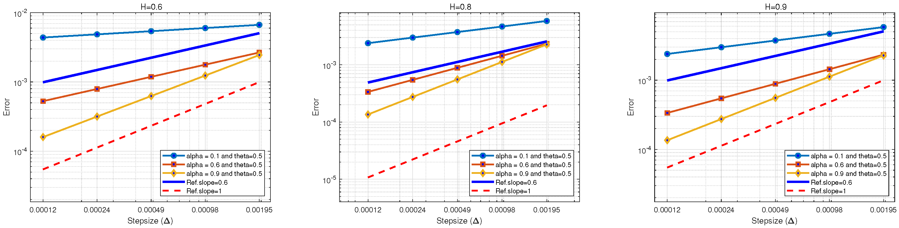
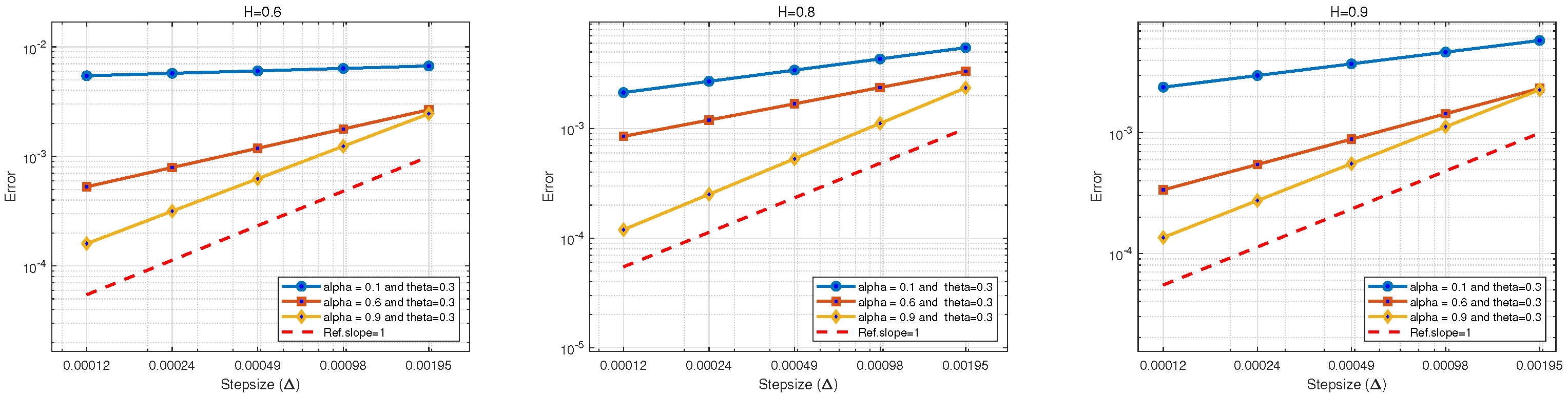
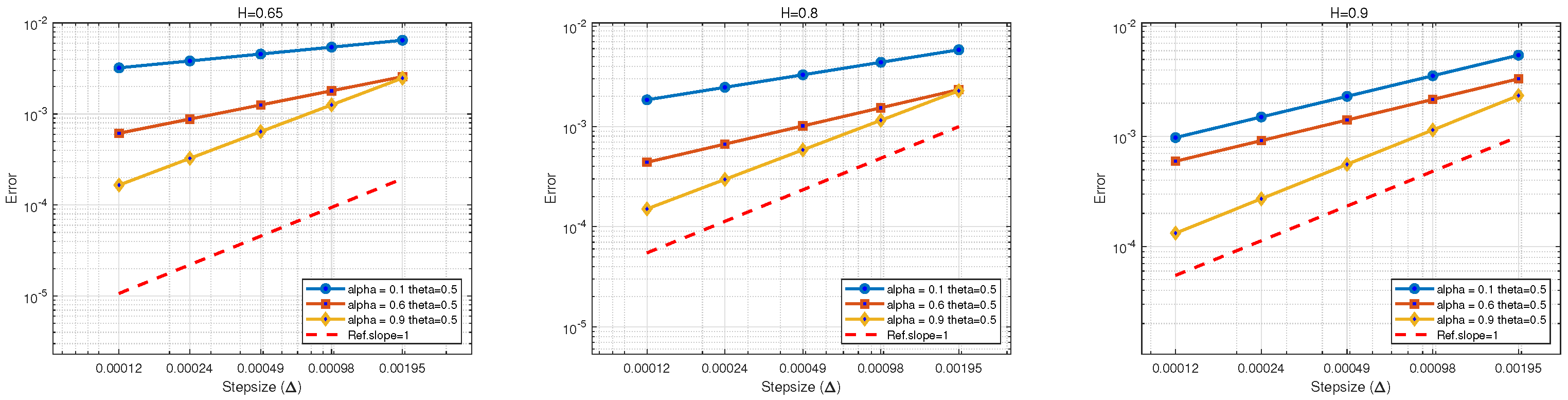
6. Numerical Experiments

In this section, we consider two examples to verify the strong convergence orders of our modified EM scheme (11). We characterize the mean—square errors at the terminal time $t_N$ as

$${\mathfrak{E}}_{h,T}=\sqrt{{\displaystyle \frac{1}{6500}}\sum _{i=1}^{6500}{|Y_h(T,{\omega }_i)-Y_{h/2}(T,{\omega }_i)|}^2},$$

where ${\omega }_i$ denotes the ith single sample path. Furthermore, the computing order is defined as

$$\mathrm{Order}={\displaystyle \frac{log({\mathfrak{E}}_{h,N}/{\mathfrak{E}}_{h/2,N})}{log2}}.$$

Example 1. 

We consider the following one-dimensional mSVIE:

$$\begin{array}{cc}\hfill y\left(t\right)=y_0+{\int }_0^t{(t-s)}^{\alpha }sin\left(y^2\left(s\right)\right)\mathrm{d}s& +{\int }_0^t{(t-s)}^{\alpha }cos\left(y^2\left(s\right)\right)\mathrm{d}{W}_s\hfill \\ & +{\int }_0^t{(t-s)}^{\alpha }cos\left(y^2\left(s\right)\right)\mathrm{d}{W}_s^H,\hfill \\ \hfill t\in [0,1],y\left(0\right)=y_0=1.\end{array}$$

It is obvious that $K_1=sin\left(y^2\left(s\right)\right)$, $K_2=cos\left(y^2\left(s\right)\right)$, and $K_3=cos\left(y^2\left(s\right)\right)$ are locally Lipschitz continuous with ${\mathcal{L}}_m=2m$ and satisfy linear growth conditions. For $p>2/\theta$, we choose

$$\nu \left(x\right)=xexp\left\{-{\displaystyle \frac{min\{2,2\alpha +1-2\theta \}}{4(p-1)}}\right\},x<1.$$

We let $\nu \left(h\right)\to \infty$ and

$$\begin{array}{cc}\hfill {\mathcal{L}}_{\nu \left(h\right)}^2{h}^{min\{2,2\alpha +1-2\theta \}}& ={\left[2\nu \left(h\right)\right]}^2{h}^{min\{2,2\alpha +1-2\theta \}}\hfill \\ & \le C{h}^{-{\displaystyle \frac{min\{2,2\alpha +1-2\theta \}}{2(p-1)}}}{h}^{min\{2,2\alpha +1-2\theta \}}\hfill \\ & \le C{h}^{{\displaystyle \frac{2p-3}{2(p-1)}}min\{2,2\alpha +1-2\theta \}}\to 0\hfill \end{array}$$

As $h\to 0$ and $p\to \infty$, the limitation expression in (15) holds, and

$${\left[{\mathcal{L}}_{\nu \left(h\right)}^2{h}^{min\{2,2\alpha +1-2\theta \}}\right]}^{-{\displaystyle \frac{p}{2(p-2)}}}\le C{h}^{-{\displaystyle \frac{p·min\{2,2\alpha +1-2\theta \}}{4(p-1)}}}\le \nu \left(h\right),$$

which means that $\nu \left(h\right)$ satisfies the condition $\nu \left(h\right)\ge {\left[{\mathcal{L}}_{\nu \left(h\right)}^2{h}^{\mathcal{O}}\right]}^{-{\displaystyle \frac{p}{2(p-2)}}}$ in Theorem 3. Figure 1 shows the mean—square errors, which become smaller as h decreases. Furthermore, we find that the Hurst parameter H has a significant impact on the convergence order, such that an increase in H results in a higher convergence order. To be specific, when $\alpha =0.9$, the strong convergence order of our modified EM method is close to 1, and for the cases of $H=0.8$ and $H=0.9$, the strong convergence orders of our modified EM method is also close to 1, respectively. To illustrate this result, we recall the example 6.1 of [5], which is similar to our Example 1. Ref. [5] verified that the mean—square errors of explicit EM method applied to SFIDEs has strong first—order convergence. They also pointed out that the convergence rate of the numerical scheme used the global Lipschitz condition, but under non—Lipschitz condition, to prove the convergence rate is still an open problem. In our test, we fixed $\theta =0.5$ and varying α, we find that an increase in α results in a higher convergence order. The convergence orders with fixed $\theta =0.3$ and varying α are shown in Figure 2 and are consistent with the theoretical analysis. These numerical results verify that the strong convergence order with the local Lipschitz condition is inherently lower than the strong convergence order $\mathcal{O}/2$ with the global Lipschitz condition.

Example 2. 

We consider the one—dimensional mixed fractional Volterra O—U (Ornstein—Uhlenbeck) equation (also see [31,32]), which is a special case of mSVIE (7) with Hölder continuous kernels. A mixed fractional Volterra Ornstein—Uhlenbeck equation is defined by

$$y\left(t\right)=y_0+{\int }_0^{t}K(t-s)(b_0+b_{1}y\left(s\right))\mathrm{d}s+{\int }_0^{t}K(t-s){\sigma }_1\mathrm{d}{W}_s+{\int }_0^{t}K(t-s){\sigma }_2\mathrm{d}{W}_s^H,$$

where $b_0,b_1,{\sigma }_1,{\sigma }_2\in \mathbb{R}$.

$$K(t-s)={\displaystyle \frac{{(t-s)}^{\alpha -\frac{1}{2}}}{\Gamma (\alpha +\frac{1}{2})}},\alpha >{\displaystyle \frac{1}{2}}.$$

According to Theorems 2 and 3, the convergence order is $\mathcal{O}/2$. We choose the following parameters:

$$y_0=1,b_0=1,b_1=-0.3,{\sigma }_1=0.1,{\sigma }_2=0.05,\alpha =0.6,H=0.65,$$

The computed results are shown in Figure 3, which demonstrates that our modified EM method for the mixed fractional Volterra O-U equation can achieve strong first-order convergence when $\alpha =0.9$.

Remark 3. 

Example 1 and Example 2 shows that the convergence rate of our modified EM scheme using the local Lipschitz condition is much more complex than using the global Lipschitz condition. Since our error $\mathit{e}\left(t\right)$ consists of two components, the first one is the error of a modified EM method, and the second one is the error of Monte Carlo method, thus, it is challenging to derive the exact orders of strong convergence under the local Lipschitz condition, even the exact orders of strong convergence is completely invisible. The precise orders of strong convergence can only be obtained under the global Lipschitz condition. We only show that the strong convergence order with the local Lipschitz condition, which is inherently lower than the strong convergence order $\mathcal{O}/2$ with the global Lipschitz condition. To prove the convergence rate under non—Lipschitz condition is still an open problem.

7. Conclusions

In this study, we relaxed the assumption of the global Lipschitz condition to the local Lipschitz condition and showed the strong convergence order of a modified EM method for mSFIEs. We first transformed the mSFIEs into an equivalent mSVIEs using a fractional calculus technique, and then proved the well—posedness of the analytical solutions to mSFIEs with weakly singular kernels. Moreover, a modified EM method was developed for numerically solving mSVIEs, and the strong convergence of the solutions was proven under local Lipschitz and linear growth conditions, as well as the well—posedness. Furthermore, we obtained the accurate convergence order of this method under the same conditions in the mean—square sense. Notably, the strong convergence order under local Lipschitz conditions is inherently lower than the corresponding order under global Lipschitz conditions. Finally, numerical experiments were presented to demonstrate that our approach not only circumvents the restrictive integrability conditions imposed by singular kernels, but also achieves a rigorous convergence order in the $L^2$ sense.

References

1. Mounir, Z.L. On the mixed fractional Brownian motion. J. Appl. Math. Stoch. Anal. 2006, 1, 1–9. [Google Scholar]
2. Mishura, Y.S. Stochastic Calculus for Fractional Brownian Motion and Related Processes; Springer: Berlin, Germany, 2008. [Google Scholar]
3. Liu, W.G.; Luo, J.W. Modified Euler approximation of stochastic differential equation driven by Brownian motion and fractional Brownian motion. Commun. Stat-Theor. Meth. 2017, 46, 7427–7443. [Google Scholar] [CrossRef]
4. Liang, H.; Yang, Z.W.; Gao, J.F. Strong superconvergence of the Euler-Maruyama method for linear stochastic Volterra integral equations. J. Comput. Appl. Math. 2017, 317, 447–457. [Google Scholar] [CrossRef]
5. Dai, X.J.; Bu, W.P.; Xiao, A.G. Well-posedness and EM approximations for non-Lipschitz stochastic fractional integro-differential equations. J. Comput. Appl. Math. 2019, 356, 377–390. [Google Scholar] [CrossRef]
6. Zhang, J.N.; Lv, J.Y.; Huang, J.F.; Tang, Y.F. A fast Euler-Maruyama method for Riemann-Liouville stochastic fractional nonlinear differential equations. Phy. D 2023, 446, 133685. [Google Scholar] [CrossRef]
7. Huang, J.F.; Shao, L.X.; Liu, J.H. Euler-Maruyama methods for Caputo tempered fractional stochastic differential equations. Int. J. Comput. Math. 2024, 101, 1113–1131. [Google Scholar] [CrossRef]
8. Liu, W.; Mao, X.R. Strong convergence of the stopped Euler-Maruyama method for nonlinear stochastic differential equations. Appl. Math. Comput. 2013, 223, 389–400. [Google Scholar] [CrossRef]
9. Song, M.H.; Hu, L.J.; Mao, X.R.; Zhang, L.G. Khasminskii-type theorems for stochastic functional differential equations. Discrete. Cont. Dyn-B 2013, 18, 1697–1714. [Google Scholar] [CrossRef]
10. Mao, X.R.; Szpruch, L. Strong convergence and stability of implicit numerical methods for stochastic differential equations with non-globally Lipschitz continuous coefficients. J. Comput. Appl. Math. 2013, 238, 14–28. [Google Scholar] [CrossRef]
11. Mao, X.R. The truncated Euler-Maruyama method for stochastic differential equations. J. Comput. Appl. Math. 2015, 290, 370–384. [Google Scholar] [CrossRef]
12. Milstein, G.N.; Tretyakov, M.V. Stochastic Numerics for Mathematical Physics; Springer: Berlin, Germany, 2004. [Google Scholar]
13. Wang, X.J.; Gan, S.Q. The tamed Milstein method for commutative stochastic differential equations with non-globally Lipschitz continuous coefficients. J. Difference Equ. Appl. 2013, 19, 466–490. [Google Scholar] [CrossRef]
14. Wang, X.J.; Gan, S.Q.; Wang, D.S. θ-Maruyama methods for nonlinear stochastic differential delay equations. Appl. Num. Math. 2015, 98, 38–58. [Google Scholar] [CrossRef]
15. Li, M.; Huang, C.M.; Hu, Y.Z. Numerical methods for stochastic Volterra integral equations with weakly singular kernels. IMA J. Numer. Anal. 2022, 42, 2656–2683. [Google Scholar] [CrossRef]
16. Hutzenthaler, M.; Jentzen, A.; Kloeden, P.E. Strong convergence of an explicit numerical method for SDEs with nonglobally Lipschitz continuous coefficients. Ann. Appl. Proba. 2012, 22, 1611–1641. [Google Scholar] [CrossRef]
17. Kamrani, M.; Jamshidi, N. Implicit Euler approximation of stochastic evolution equations with fractional Brownian motion. Commun. Nonlinear Sci. Numer. Simu. 2017, 44, 1–10. [Google Scholar] [CrossRef]
18. Anh, P.; Doan, T.; Huong, P. A variation of constant formula for Caputo fractional stochastic differential equations. Stat. Proba. Lett. 2019, 145, 351–358. [Google Scholar] [CrossRef]
19. Ford, N.J.; Pedas, A.; Vikerpuur, M. High order approximations of solutions to initial value problems for linear fractional integro-differential equations. Fract. Calc. Appl. Anal. 2023, 26, 2069–2100. [Google Scholar] [CrossRef]
20. Mao, X.R. Stochastic Differential Equations and Applications; Horwood Pub Ltd.: Chichester, UK, 1997.
21. Higham, D.J.; Mao, X.R.; Stuart, A. Strong convergence of Euler-type methods for nonlinear stochastic differential equations. SIAM J. Numer. Anal. 2003, 40, 1041–1063. [Google Scholar] [CrossRef]
22. Yang, Z.W.; Yang, H.Z.; Yao, Z.C. Strong convergence analysis for Volterra integro-differential equations with fractional Brownian motions. J. Comput. Appl. Math. 2021, 383, 113156. [Google Scholar] [CrossRef]
23. Liu, W.G.; Jiang, Y.; Li, Z. Rate of convergence of Euler approximation of time-dependent mixed SDEs driven by Brownian motions and fractional Brownian motions. AIMS Math. 2020, 5, 2163–2195. [Google Scholar] [CrossRef]
24. Mishura, Y.; Shevchenko, G. Mixed stochastic differential equations with long-range dependence: Existence, uniqueness and convergence of solutions. Comput. Math. Appl. 2012, 64, 3217–3227. [Google Scholar] [CrossRef]
25. Nualart, D. The Malliavin Calculus and Related Topics (Probability and Its Applications), 2nd ed.; Springer: Berlin, Germany, 2006. [Google Scholar]
26. Biagini, F.; Hu, Y.Z.; Øksendal, B.; Zhang, T.S. Stochastic Calculus for Fractional Brownian Motion and Applications; Cambridge University Press: London, UK, 2008. [Google Scholar]
27. Li, L.; Liu, J.G.; Lu, J.F. Fractional stochastic differential equations satisfying fluctuation-dissipation theorem. J. Stat. Phy. 2017, 169, 316–339. [Google Scholar] [CrossRef]
28. Costabile, C.; Massabó, I.; Russo, E.; Staino, A. Lattice-based model for pricing contingent claims under mixed fractional Brownian motion. Commun. Nonlinear Sci. Num. Sim. 2023, 118, 107042. [Google Scholar] [CrossRef]
29. Lan, G.Q.; Xia, F. Strong convergence rates of modified truncated EM method for stochastic differential equations. J. Comput. Appl. Math. 2018, 334, 1–17. [Google Scholar] [CrossRef]
30. Qin, Y.M. Integral and Discrete Inequalities and Their Applications, Volume I: Linear Inequalities; Springer: Berna, Switzerland, 2016. [Google Scholar]
31. Rao, B.L.S.P. Parametric estimation for linear stochastic differential equations driven by mixed fractional Brownian motion. Stoch. Anal. Appl. 2018, 36, 767–781. [Google Scholar] [CrossRef]
32. Alazemi, F.; Douissi, S.; Sebaiy, K.E. Berry-Esseen bounds and asclts for drift parameter estimator of mixed fractional Ornstein-Uhlenbeck process with discrete observations. Theor. Proba. Appl. 2019, 64, 401–420. [Google Scholar] [CrossRef]
Figure 1. (Left): the mean—square errors of the modified EM scheme with θ = 0.5 and H = 0.6 . (Middle): the mean—square errors of the modified EM scheme with θ = 0.5 and H = 0.8 . (Right): the mean—square errors of the modified EM scheme with θ = 0.5 and H = 0.9 .
Fractalfract 09 00296 g001
Figure 2. (Left): the mean—square errors of the modified EM scheme with θ = 0.3 and H = 0.6 . (Middle): the mean—square errors of the modified EM scheme with θ = 0.3 and H = 0.8 . (Right): the mean—square errors of the modified EM scheme with θ = 0.3 and H = 0.9 .
Fractalfract 09 00296 g002
Figure 3. (Left): the mean—square errors of the modified EM scheme with θ = 0.5 and H = 0.65 . (Middle): the mean—square errors of the modified EM scheme with θ = 0.5 and H = 0.8 . (Right): the mean—square errors of the modified EM scheme with θ = 0.5 and H = 0.9 .
Fractalfract 09 00296 g003
Disclaimer/Publisher’s Note: The statements, opinions and data contained in all publications are solely those of the individual author(s) and contributor(s) and not of MDPI and/or the editor(s). MDPI and/or the editor(s) disclaim responsibility for any injury to people or property resulting from any ideas, methods, instructions or products referred to in the content.