The Application of Abstract Algebra in Operational Calculus

Abstract

This paper is dedicated to elucidating the abstract algebraic structure of operational calculus theory. Based on abstract algebra and operational calculus, the operator algebra theory of Mikusiński has been revised. We restate the concept of Mikusiński’s operator field as a convolutional field and define a new concept of operator field with the differential operator p as the core, effectively overcoming the confusion between the concepts of operators and functions, which represents the limitation of traditional theory. In addition, the classical Laplace transform is integrated into our theory in a homomorphic form, revealing the principle that the Laplace transform is compatible with operational calculus theory.

1. Introduction

This article is dedicated to the abstract algebraic foundation of operational calculus theory and clarifies a fundamental question: Why can the Laplace transform be perfectly matched with operational calculus?

Operational calculus is an important component of mathematical physics [1,2,3]. In 1893, Heaviside [1] creatively proposed the differential operator symbol p, marking the establishment of this discipline. Over the past 100-plus years, people have never ceased to explore the mysteries hidden within it [4,5,6]. From solving differential equations to handling fractional calculus, operational calculus has frequently emerged [7,8,9]. In recent years, operational calculus has been widely applied in the study of physical fractal spaces and fractal operators, which possess fractional orders and demonstrate non-local properties [10,11,12,13]. However, similar to the history of calculus: historically, calculus has been widely applied, but its logical foundation was flawed. Currently, the logical foundation of operational calculus remains questionable. To solidify its logical foundation, it needs to be abstracted to a sufficient degree.

Abstract algebra is the crown of pure mathematics. The theory of groups founded by Galois in the 19th century marked the origin of abstract algebra. The current framework of abstract algebra is attributed to the foundational contributions of Noether. Abstract algebra studies algebraic structures and attaches great importance to the generality of propositions and the rigor of logic. It is precisely because of the generality of propositions and the high degree of conceptual condensation that abstract algebra plays a fundamental role in pure mathematics. However, this high degree of condensation also brings about difficulties in understanding, and thus its application in practical fields is very limited.

The theory of operational calculus originated in mathematical physics and was far removed from abstract algebra. However, as research advanced, the definitions and operational rules of the basic concepts of operational calculus gained attention. The introduction of abstract algebra into operational calculus became increasingly necessary. This pioneering work was accomplished by Mikusiński [6] in the mid-20th century. Mikusiński reduced operators to an algebraic structure, achieving the combination of the two. This idea is undoubtedly pioneering. Mikusinski’s innovation has been systematically reviewed by Brychkov et al. [14]. Notable developments include Mikusiński’s [6] work on ordinary differential equations with variable coefficients, Gutterman’s [15] application to partial differential equations, and Luchko’s [16,17] generalization to fractional-order ordinary differential equations. In recent years, Bengochea et al. [18] examined operational calculus from the perspective of linear algebra and proposed a modified shift operator operational calculus method in the abstract space of formal Laurent series. Moreover, Arran Fernandez et al. [19] applied it to fractional calculus, thereby efficiently solving fractional differential equations. Meanwhile, the work by Glaeske et al. [20] stands as one of the latest compiled textbooks on operational calculus.

However, with the development of the kernel function method for operators, people gradually realized that the logical foundation of the operator algebra was incomplete and there were ambiguities. At the same time, Mikusiński’s operator algebra did not provide a general method for determining the kernel function from the operator.

To overcome the above limitations, Yu et al. [21], through induction and with the aid of integral transforms, revealed the correlation between kernel functions and operators, and they summarized the general solution process of the operator kernel function method. However, Yu et al. [21] focused on practical applications and did not pay much attention to the algebraic structure. Therefore, the ambiguities in Mikusiński’s operator algebra have not been clarified.

The root cause of the problem lies in the insufficient rigor of the algebraization of calculus operations. People merely focused on some applications of algebraic structures but neglected the strict analysis of the algebraic structures themselves. As a result, the derived algebraic definitions are overly empirical and lack logical rigor and completeness. This constitutes the motivation of this paper.

This paper introduces rigorous abstract algebra and corrects and reshapes Mikusiński operator algebra. We integrated the research ideas of previous scholars, reconstructed the operator domain, and constructed a clear and concise algebraic system. With this algebraic system, we elaborated on the existing operator kernel function method in detail, strengthening its logical foundation.

The text includes the following contents: Section 2 reviews the concepts of abstract algebra. Section 3 introduces Mikusiński’s research approach, redefines the operator domain, and renames it as the convolution domain. Section 4 discusses the properties of the convolution domain and explains the connotation of the operator f/g. Section 5 studies the p operator and defines a new concept of operator domain, distinguishing it from the corresponding convolution domain of which the operator f/g belongs to. Section 6 characterizes the Laplace integral transform as a homomorphism and completes the entire logical framework. Section 7 demonstrates the effectiveness of the abstract operator algebra system through the example of equation solving.

2. Basic Concepts of Abstract Algebra

First, it is necessary to review the abstract algebraic concepts used in this paper. The content of this section is based on Atiyah’s “Introduction to Commutative Algebra” [22].

Definition 1.

A commutative ring with identity $A$ is a set equipped with two binary operations (addition and multiplication) such that:

(1) 

$A$ forms an abelian group under addition.

(2) 

Multiplication is commutative and associative:

$$xy=yx, (xy)z=x(yz),$$

and multiplication distributes over addition:

$$x(y+z)=xy+xz,(y+z)x=yx+zx.$$

(3) 

Multiplication has an identity element (denoted as 1), satisfying

$$\forall x\in A, x1=1x=x.$$

In the subsequent chapters, the term “ring” will refer specifically to a commutative ring with identity. Furthermore, by the properties of abelian groups, it is evident that all rings also contain an additive identity element, denoted as 0, which satisfies

$$x\in A, 0+x=x+0=x$$

(1)

There may exist a class of elements that divide zero in a ring, i.e.,

$$y\ne 0, xy=0$$

(2)

These elements are defined as zero divisors. A ring that contains no zero divisors is called an integral domain.

Definition 2.

A ring homomorphism is a mapping f from a ring A to a ring B that satisfies the following properties:

(1) 

Preservation of addition: $f(a_1+a_2)=f(a_1)+f\left(a_2\right)$.

(2) 

Preservation of multiplication: $f(a_1{a}_2)=f(a_1)f\left(a_2\right)$.

(3) 

Preservation of the multiplicative identity:

$f(1_A)=1_B$, where $1_A$ and $1_B$ are the multiplicative identities of rings A and B.

It is evident that f preserves the invariance of addition, multiplication, and the multiplicative identity. From property (1), it is straightforward to deduce that f also satisfies

$$f(0_A)=0_B, f(-a)=-f(a)$$

(3)

In general, an element x in a ring does not necessarily possess a corresponding multiplicative inverse y (i.e., an element such that $x·y=1$). However, many common mathematical structures inherently include the existence of multiplicative inverses, such as the rational numbers $\mathbb{Q}$ and the real numbers $ℝ$. To describe such structures, the concept of a field is introduced.

Definition 3.

A field is a commutative ring with identity in which every nonzero element has a multiplicative inverse.

By defining scalar multiplication over a field, one obtains the commonly used mathematical structure known as a vector space. When the algebraic structure of the scalars is relaxed from a field to a ring, the concept of a module emerges.

Definition 4. 

A module M over a ring A (also called an A-module) is an abelian group equipped with a scalar multiplication operation that satisfies the following properties for all $r,s\in A$ and $m,n\in M$:

(1) 

Distributivity of scalar multiplication:

$$r·(m+n)=r·m+r·n,(r+s)·m=r·m+s·m.$$

(2) 

Compatibility of scalar multiplication with ring multiplication:

$$(r·s)·m=r·(s·m).$$

(3) 

Identity element of scalar multiplication:

$1_A·m=m$, where $1_A$ is the multiplicative identity of the ring A.

One of the most classic examples of a module is when A is a field k. In this case, an A-module becomes a k-vector space.

Finally, we introduce the theory of fractionation of rings. In order to construct “fractions” within a ring, we introduce the concept of division. The ring composed of such fractions is called a fractional ring. The construction of fractional ring relies on the concept of a multiplicatively closed subset, which generalizes the notion of denominators. The definition is as follows:

Definition 5.

Let $A$ be a ring. A subset $S\subseteq A$ is called a multiplicatively closed subset of $A$ if $S$ is close under multiplication and contains the multiplicative identity.

The concept of “fractions” arises from an equivalence relation defined on the set $A\times S$ in the following manner:

$$(a,s)\equiv (b,t)\iff (at-bs)u=0, \mathrm{for} \mathrm{specific} u\in S$$

(4)

Obviously, this relation is reflexive and symmetric. Therefore, to demonstrate that it is an equivalence relation, it suffices to verify transitivity. Suppose

$$(a,s)\equiv (b,t), (b,t)\equiv (c,u)$$

(5)

Then

$$\exists v,w\in S, \mathrm{s}.\mathrm{t}. (at-bs)v=0, (bu-ct)w=0$$

(6)

By combining the two equations and eliminating b, we obtain

$$(au-cs)tvw=0.$$

(7)

Noticing S is close under multiplication, $tvw\in S$, there is

$$(a,s)\equiv (c,u).$$

(8)

Thus, transitivity is verified. We denote the equivalence class $(a,s)$ as ${\displaystyle \raisebox{1ex}{$a$}\!\left/ \!\raisebox{-1ex}{$s$}\right.}$, then denote $S^{-1}A$ by the set composed of all equivalence classes. Addition and multiplication on “fractions” ${\displaystyle \raisebox{1ex}{$a$}\!\left/ \!\raisebox{-1ex}{$s$}\right.}$ are defined as follows:

$$({\displaystyle \raisebox{1ex}{$a$}\!\left/ \!\raisebox{-1ex}{$s$}\right.})+({\displaystyle \raisebox{1ex}{$b$}\!\left/ \!\raisebox{-1ex}{$t$}\right.})={\displaystyle \raisebox{1ex}{$(at+bs)$}\!\left/ \!\raisebox{-1ex}{$st$}\right.}, ({\displaystyle \raisebox{1ex}{$a$}\!\left/ \!\raisebox{-1ex}{$s$}\right.})({\displaystyle \raisebox{1ex}{$b$}\!\left/ \!\raisebox{-1ex}{$t$}\right.})={\displaystyle \raisebox{1ex}{$ab$}\!\left/ \!\raisebox{-1ex}{$st$}\right.},$$

(9)

so we introduced the ring structure on $S^{-1}A$, with the name fractional ring, also noted as $S^{-1}A$.

It is important to note that while fractional ring introduces the concept of “fractions”, the absence of multiplicative inverses for all elements still prevents the full implementation of division. To address this limitation, we can construct fractional field, which ensures that every nonzero element has a multiplicative inverse, thereby enabling a complete division operation. This construction is achieved through a fundamental theorem in algebra.

Theorem 1. 

If A is an integral domain and $S={\displaystyle \raisebox{1ex}{$A$}\!\left/ \!\raisebox{-1ex}{$\left\{0\right\}$}\right.}$, then fractional ring $S^{-1}A$ is a field, called the fractional field of A.

The proof of Theorem 1 can be easily found in Atiyah’s “Introduction to Commutative Algebra” [22].

3. The Derivation of Convoluted Field

Following Mikusiński’s [6] approach, we first aim to clarify the concept of the operator field. As the central concept in former operator algebra theory, the operator field serves as the foundation for defining other notions. However, traditional formulation of the operator field contains certain ambiguities. Below, we will reformulate Mikusiński’s theory using modern algebra to develop a clearer and more rigorous operator algebra theory.

Let us examine the Mikusiński operator field. The construction of algebraic structures is fundamentally based on the concept of sets. Therefore, before discussing an algebraic structure, it is essential to clarify the objects on which this structure is imposed. This is precisely the approach taken by Mikusiński in his work.

To begin the discussion of operator algebra, Mikusiński defined a specific function set. This function set remain fundamental objects of study in operational calculus theory and are referred to as the Mikusiński function set $𝒦$. The definition of $𝒦$ is as follows:

Definition 6.

Mikusiński function set $𝒦$ consists all the functions defined on the interval $(0,+\infty )$ satisfying:

(1) 

The function f(t) has a set of discontinuities with measure zero.

(2) 

For any t > a, the integral of the function f(t) is bounded.

As a fundamental definition of operational calculus, we still use the function set $𝒦$ in our discussion.

With the foundational set $𝒦$ established, we can now define algebraic structures on it. The desired algebraic framework is constructed by introducing operations on $𝒦$. Mikusiński introduced addition and convolution as the fundamental operations on $𝒦$, leading to the core algebraic structure of operator algebra, known as the Mikusiński ring M. Compared with common function rings, it can be seen the multiplication of M corresponded to convolution, which is one of the most significant aspects of M worthy of in-depth study. Since convolution directly reflects the essential characteristics of M, we refer to M as the convoluted ring. The specific definition of the convoluted ring is as follows:

Definition 7.

The convoluted ring M = (K, +, ∗) where + is the addition operation and ∗ is the convolution operation.

Definition 8.

The convolution of f and g, denoted f ∗ g, is defined as

$$f\ast g={\displaystyle \underset{0}{\overset{t}{\int }}f(t-\tau )}g(\tau )d\tau .$$

(10)

It is obvious that convolution obeys laws of commutative, associative, and distributes over addition, satisfying the requirements of the ring for arithmetic properties, which means the concept of M is clear and distinct.

When mathematicians introduce new concepts, they invariably seek out the “good” properties these concepts might possess, allowing the new structures to be connected to existing algebraic systems. By leveraging these systems, more information about the new structures can be obtained. The Mikusiński ring M is an exceptionally “good” structure, as highlighted by Titchmarsh’s theorem.

Theorem 2

(Titchmarsh’s). f ∗ g = 0 only if f = 0 or g = 0.

The zeroization problem is a central issue in algebra. The most straightforward form of zeroization is multiplication by “0”. In algebra, there often exist nonzero elements that, when multiplied by certain other elements, yield zero. Such elements are called zero divisors. The presence of zero divisors in an algebraic structure can introduce significant complications. The “goodness” of Titchmarsh’s theorem lies in the fact that only “0” can annihilate other elements through multiplication, meaning there are no zero divisors. Such a “good” structure, which lacks zero divisors, is called an integral domain in algebra. Therefore, we can provide an algebraic corollary of Titchmarsh’s theorem.

Corollary 1.

Convoluted ring M is an integral domain.

Integral domains possess many excellent properties in algebra. Using Theorem 1, we can perform the fractionalization of the convoluted ring M, resulting in a field noted as $S^{-1}M$ where every nonzero element has a multiplicative inverse. $S^{-1}M$ is precisely the operational field defined by Mikusiński who utilized the concept of inverses in this field to define division, completing the extension of the concept from functions to operators. In honor of Mikusiński’s contributions, this field is often referred to as the Mikusiński field. Of course, $S^{-1}M$ can also be called the convoluted field as convolution still remains the most fundamental feature.

In this way, we have arrived at Mikusiński’s conclusions from an algebraic perspective. The ordinary methods (by Mikusiński) used precise mathematical language to define division and derive the concept of the convoluted field from the convolution ring M. Unlike traditional approach, the algebraic narrative and construction presented here are more concise and better reveal the essence behind the concepts. This demonstrates the superiority of algebra in simplifying and clarifying complex ideas.

4. Properties of Convoluted Field

Compared to the convoluted ring M, the introduction of division in the convoluted field gives rise to new concepts and properties. Mikusiński leveraged these new results in the convolution field to construct his operator algebra theory. However, the ambiguities in his theory can also be traced back to this point. Therefore, a thorough analysis of the structure of the convolution field is essential.

For a field structure, the first algebraic focus is on the specific forms of its additive and multiplicative identity elements. These elements represent the invariants of addition and multiplication in the field, forming the foundation for all operations within the field. We can determine the “0” and “1” of convoluted field using the following expressions:

$$0_{S^{-1}M}+f=f, 1_{S^{-1}M}\ast f=f, f\in S^{-1}M.$$

(11)

Since addition of the convoluted field is defined consistently with addition in the real number field, the zero element of convoluted field is essentially a generalization of the real number 0 in the context of functions. Specifically, the zero element is the constant function 0(t) = 0 for all t ≥ 0.

On the other hand, the identity element of multiplication must be determined by solving the convolution equation listed before. However, this equation is inherently complex, but fortunately, we can use existing results to directly determine its solution.

We notice the Dirac delta function δ(t) satisfies:

$$\delta (t)\ast f=f, \forall f\in S^{-1}M.$$

(12)

This formula indicates that Dirac delta function δ(t) is a solution of identity element equation. Considering the uniqueness of identity element in algebra, we confirm the Dirac delta function as the identity element of convoluted field.

The fact that the Dirac delta function δ(t) is the identity element in the convoluted field is a result that aligns well with intuition. This conclusion is supported by related research in operational calculus, where δ(t) has long been a central object of study. Now, from the perspective of foundational algebra, we can confirm the validity of using δ(t) in these studies. Historically, δ(t) was regarded as a mathematical concept derived from physics. However, it now reveals a purely mathematical significance. It should be noted, though, that this result was not explicitly covered in Mikusiński’s original research. This once again demonstrates the power of abstract algebra in unifying and clarifying mathematical concepts.

Next, we discuss the concepts of fractions and division in the convoluted field. These concepts arise naturally from the construction of the fractional field. A key aspect of this construction is the equivalence relation used to define fractions:

$$(a,s)\equiv (b,t)\iff at-bs=0,$$

(13)

which corresponds to the equivalence of fractions. Consequently, we can denote the equivalence class $(a,s)$ as ${\displaystyle \raisebox{1ex}{$a$}\!\left/ \!\raisebox{-1ex}{$s$}\right.}$. The addition and multiplication operations on the convoluted field $S^{-1}M$ are precisely the operations that fractions adhere to

$${\displaystyle \frac{a}{s}}+{\displaystyle \frac{b}{t}}={\displaystyle \frac{at+bs}{st}}, {\displaystyle \frac{a}{s}}\ast {\displaystyle \frac{b}{t}}={\displaystyle \frac{ab}{st}}.$$

(14)

It can be observed that the properties of fraction operations derived from abstract algebra are entirely consistent with Mikusiński’s definition.

Division is defined through the concept of inverses in the field of fractions, while inverses are directly defined by the identity element. The definition of an inverse can be generally expressed in algebraic terms by the equation

$$a{a}^{-1}=a^{-1}a=1.$$

(15)

By utilizing the identity element in convoluted field, we can directly derive the representation of the inverse element illustrated in (16).

$${\displaystyle \underset{0}{\overset{t}{\int }}f(t-\tau )f^{-1}}(\tau )d\tau ={\displaystyle \underset{0}{\overset{t}{\int }}{f}^{-1}(t-\tau )f}(\tau )d\tau =\delta (t).$$

(16)

Thus, the division in convoluted field can be expressed as the convolution of inverses, as (17)

$${\displaystyle \frac{f}{g}}=f{g}^{-1}={\displaystyle \underset{0}{\overset{t}{\int }}f(t-\tau )g^{-1}}(\tau )d\tau .$$

(17)

By solving Equation (17), we can obtain the formula for the inverse element. Substituting this into Equation (17) yields the formula for division, which allows us to directly compute the quotient of the known functions f and g, without the step to calculate the inverse.

Obviously, this form of division and convolution are mutually inverse operations. To highlight this symmetry, we can refer to division in the convoluted field as “divolution”.

With the introduction of division, we can now examine the results of this operation. Just as the introduction of division in the integer ring extends the integers to the rational numbers, the convoluted field $S^{-1}M$, compared to the convoluted ring M, introduces a new class of objects f/g due to the inclusion of divolution quotients. Mikusiński undoubtedly recognized this and named these new objects operators. We can see the reasoning behind this naming from the following expression:

$$g{\displaystyle \frac{f}{g}}=gf{g}^{-1}=f\delta (t)=f.$$

(18)

It is not difficult to see that the expression f/g reflects an operation that transforms the function g into the function f, which aligns well with the intuitive meaning of an operator. However, this seemingly reasonable definition is also the source of many ambiguities in operator algebra. Though it is permitted to assign names to concepts arbitrarily through definitions, the practical value of such definitions lies in their consistency with existing logical systems and their compatibility with established knowledge frameworks. Unfortunately, the broad and vague concept of an operator defined in this way does not seamlessly integrate with existing logical systems, leading to several challenges. The details are as follows.

The incompatibility highlighted earlier is further reflected in another object that was already well-defined as an operator before the introduction of the convoluted field: the differential symbol p. Clearly, the differential symbol p does not belong to the convoluted field $S^{-1}M$. The most direct evidence is that the action of p on functions is defined through composition rather than convolution, and the multiplication it satisfies is not convolution. As a result, after Mikusiński’s definition, the single concept of an operator refers to two distinct types of objects, leading to inevitable confusion.

The situation becomes even more problematic when Mikusiński attempts to unify the convoluted field with the existing operator calculus by equating operators involving p with operators of the form f/g in the convoluted field. This approach blends two fundamentally different types of operators—those that follow composition rules p and those that follow convolution rules f/g—into a single framework through the use of equalities. As a result, the operator algebra system becomes entangled, leading to significant ambiguities and inconsistencies.

Since the issue arises from the definition itself, the solution is relatively straightforward: we only need to rename f/g to avoid confusion. While the previous discussion critiques Mikusiński’s definition to some extent, it is important to acknowledge that Mikusiński’s understanding of f/g is actually quite appropriate, except the overgeneralization of the concept. Therefore, we can resolve the issue by adding a specific adjective to Mikusiński’s definition to clarify the context.

Noticing f/g belongs to the convoluted field, we can refer to it as a convoluted operator to distinguish it from operators like p that follow ordinary multiplication. If the term convolution operator is still prone to confusion with general operators, we can alternatively call it a fractional function.

With the introduction of the fractional function concept, we can now address some practical problems. One of the most classic examples is the definition of scalar multiplication in the convoluted field. Similar to the construction of ordinary scalar multiplication, Mikusiński defined a class of scalar operators that satisfy the convolution equation:

$$fg=kg={\displaystyle \underset{0}{\overset{t}{\int }}f(t-\tau )g}(\tau )d\tau =kg(t).$$

(19)

Solving the equation yields the specific expression of the numerical operator:

$$f={\displaystyle \frac{k}{1}}.$$

(20)

Furthermore, it can be verified that all numerical operators form a field that satisfies addition and convolution, which is called a numerical operator field ${\displaystyle \raisebox{1ex}{$ℝ$}\!\left/ \!\raisebox{-1ex}{$1$}\right.}$. It is not difficult to see that the numerical operator field is a subfield of the convoluted field.

In this way, multiplication can be characterized as the convolution of elements in the numerical operator field with elements in the convoluted field, which can be considered algebraically as a mapping:

$$\mu :{\displaystyle \raisebox{1ex}{$ℝ$}\!\left/ \!\raisebox{-1ex}{$1$}\right.}\times S^{-1}M\to S^{-1}M.$$

(21)

Therefore, the convolution field with the introduction of scalar multiplication can be described by $(S^{-1}M,\mu )$. We can verify that this structure satisfies the definition of a module, specifically a ${\displaystyle \raisebox{1ex}{$ℝ$}\!\left/ \!\raisebox{-1ex}{$1$}\right.}$-module. This means that the convolution field, equipped with scalar multiplication, is not just a field but also a module over ${\displaystyle \raisebox{1ex}{$ℝ$}\!\left/ \!\raisebox{-1ex}{$1$}\right.}$. This is a subtle but important point that Mikusiński did not explicitly clarify in his work.

5. Construction of the Operational Field

The convolution field $S^{-1}M$ clarifies the meaning of the operator f/g by providing a rigorous algebraic framework for its definition and manipulation. Now, another concept that requires clarification is the operator p. Just as f/g is built on an algebraic structure, the operator p also corresponds to a specific algebraic structure, which is the main focus of this section.

To study the algebraic structure of the operator p, we first need to determine the basic set on which this structure is built. By organizing and summarizing existing operator algebra theories, we can abstract the basic set corresponding to the operator p. In operator algebra theory, operators involving p noting T(p) are divided into two categories. One type is regular operators that can be calculated using general differential rules, namely, p and its powers. The other type is singular operators that cannot be calculated using existing differential rules such as the classical $e^{\sqrt{p}}$. Regardless of whether an operator is regular or singular, we can always view T(p) as a mapping of the operator p. For example

$$e^{\sqrt{p}}\iff T({\left.x\right|}_p)=e^{\sqrt{x}}, p^3\iff T({\left.x\right|}_p)=x^3.$$

(22)

We can see that regular operators are viewed as a special case of mappings where the mapping is taken to be a power mapping.

These mappings T(p) are undoubtedly one-to-one, allowing us to interpret them as functions. Consequently, the specific set of operators T(p) is transformed into a general set of functions. However, this does not mean that the basic set is fully determined. Since the category of function sets is too broad, we need to identify the common characteristics of these mappings to further refine the basic set. At this point, the fundamental principle of operator series comes into play. This principle assumes that all operators T(p) involving p can be represented as power series, meaning that the corresponding functions can be expanded into power series. The equivalent condition for a power series expansion is that the function is infinitely differentiable, or “smooth”. Therefore, the basic set corresponding to operators T(p) involving p is determined to be the set of smooth functions $C^{\infty }(p)$. Unlike the usual smooth functions that take x as the independent variable, here, the smooth functions T(p) are functionals of the differential operator p, placing them in the realm of functional analysis. This once again demonstrates the extension of concepts.

After determining the basic set, we can now equip it with operations. To ensure the existence of a transformation relationship between the convolution field and the algebraic structure of T(p) operators, we introduce addition and multiplication operations on the set of smooth functions, thereby constructing a ring structure. It is important to note that, in existing operator algebra theories, when T(p) operators act on functions, they do so through composition rather than convolution. Similarly, the multiplication of two T(p) operators T₁(p) and T₂(p) is simply the product of the operators. Therefore, the multiplication defined in the set of smooth functions is identical to multiplication in the real number field.

If we replace the operator p with a variable x, the resulting structure is the field of smooth functions familiar from mathematical analysis. Since the substitution of p with x does not affect the algebraic structure, the algebraic structure constructed from T(p) operators is also a field, called the operator field. In honor of Heaviside, we also refer to this field as the Heaviside field, denoted by H.

The Heaviside field H itself is not inherently complex. By algebraically formalizing the equivalence between the operator p and the variable x, we establish an isomorphism $\varphi :C^{\infty }\to H$ between the function field and the Heaviside field H. This means that the properties of H can be transformed into properties of the function field by $\varphi$. Consequently, the properties of the Heaviside field H are equivalent to those of the field of smooth functions, which have been extensively studied in calculus. Therefore, from an algebraic perspective, the Heaviside field can be considered well-understood.

It is worth noting that, since the addition and multiplication operations in H are classical, the identity element and zero element are consistent with the classical 1 and 0, respectively. Furthermore, the differential operator p is completely equivalent to a polynomial variable, simplifying its algebraic treatment.

The most striking aspect of the Heaviside field is its designation as an operator field. Mikusiński had already defined the concept of an operator field, but the newly defined operator field (the Heaviside field) is not consistent with Mikusiński’s original definition. Specifically, the former is a field composed of T(p), while the latter contains convolution operators, such as f/g.

This distinction is precisely the purpose of this work: by redefining the concept of an operator as T(p), we can refine the original concept of the operator field into the convoluted field. This refinement simplifies and clarifies the operator algebra system, making it more precise and elegant.

Redefining the concept of an operator as an operator involving p (i.e., T(p)) offers two key advantages:

• In the Heaviside field H, every element is an operator involving p, meaning they all exhibit operator properties. In contrast, the convoluted field contains a significant number of elements that are not operators but rather functions. This means that the operator properties in the convoluted field are insufficient or incomplete.
• The type of operators first proposed by Heaviside were those involving p. Operators based on multiplication were introduced earlier and are more aligned with Heaviside’s original interpretation of operators, rather than the later-developed convolution operators.
• Through the above discussion, it is evident that the convoluted field is an algebraic structure that encompasses two distinct concepts: functions and convolution operators. This is precisely what we aim to avoid. However, we can also interpret the functions in the convoluted field as operator-like functionals, but this operator property arises from the combination of two factors, rather than being intrinsic to the elements themselves, as in the Heaviside field.
• Thanks to the fact that multiplication in the convoluted field is represented by convolution, functions in the convoluted field, when participating in operations, act as convolution kernels that transform one function into another. From this perspective, functions exhibit an operator-like property. Similarly, the operator property of convolution operators also stems from convolution. When considered independently of convolution, convolution operators lose their operator-like nature and instead represent an extension of the concept of functions. This is why this work advocates referring to convolution operators as fractional functions.
• Strictly speaking, there is only one type of element in the convoluted field: fractional functions. This is because fractional functions, as an extension of the concept of functions, encompass ordinary functions. Thus, the convolution field is actually a special structure composed of fractional functions, but due to the convolution operation, it manifests as operator-like functionals. Mikusiński failed to recognize this distinction. By conflating convolution with fractional functions, he introduced a confused concept of operators.

6. L-Homomorphism

At this point, we have separated the originally ambiguous operational field into two distinct and clear algebraic structures, thereby clarifying the concepts. However, operational calculus is a formal method for solving differential equations, and its core essence lies in leveraging the relationship between operators involving p (e.g., T(p)) in the operational field and functions in the convoluted field to solve equations. Although Mikusiński conflated the two, he introduced an equivalence between T(p) and convoluted operators, enabling their interaction. In contrast, the convolution field and operator field we constructed are isolated from each other so far and cannot be directly transformed. Therefore, the main goal of this section is to establish a correspondence between the two, completing the final missing link in the operator algebra theory.

Using the relationships between algebraic structures to characterize the properties of research objects has always been at the core of algebra. The concept developed for this purpose is the well-known homomorphism. This idea is no exception in the context of the convoluted field and the operational field. Homomorphisms ensure the synchronization of operations, which manifests as follows: when solving equations using the operational calculus method, operators are often decomposed to optimize computations. In this process, it is assumed that operators and their corresponding functions can be decomposed synchronously. Therefore, the correspondence between the two can be fully characterized by a homomorphism between them.

With this in mind, we define a homomorphism from the convoluted field to the operational field:

$$\varphi :S^{-1}M\to H.$$

(23)

Thus, the problem of establishing a correspondence between the convoluted field and the operational field is transformed into the study of the properties of the homomorphism ϕ.

After defining the formal homomorphism ϕ, we can explore the possible forms of this mapping. This is the basis for Mikusiński’s definition of operator equality. By leveraging the form of the homomorphism, we can derive a general formula for computing equivalent operators, which Mikusiński did not provide. This mapping can be derived by substituting the basic definition of a homomorphism into the specific algebraic structures.

Based on the fundamental definition of a homomorphism, the homomorphism ϕ between the convoluted field and the operational field must satisfy the following conditions:

$$\begin{gathered} \forall f_1,f_2\in S^{-1}M, \exists T_1,T_2\in H, \\ \mathrm{s}.\mathrm{t}. \phi (f_1+f_2)=T_1+T_2, \phi (f_1{f}_2)=T_1{T}_2, \phi (1_{S^{-1}M})=1_H. \end{gathered}$$

(24)

Furthermore, the addition, multiplication, zero element, and identity element in both the convoluted field and the operational field can be explicitly represented. This allows us to derive the constraints that the homomorphism ϕ must satisfy.

$$\phi (f_1+f_2)=T_1+T_2, \phi (f_1\ast f_2)=T_1{T}_2, \phi (\delta (t))=1.$$

(25)

Clearly, directly solving the above equations is no easy task. Therefore, we can reverse our approach and look for results that satisfy these equations among existing transformations. It is not difficult to see that the constraints provided are essentially the classical convolution theorem. Additionally, the properties of the Dirac delta function mentioned above lead us to realize that the Laplace transform and Fourier transform are potential candidates. For comparison, let us list some properties of the Laplace transform and Fourier transform below (

Table 1. Properties of the Laplace transform and Fourier transform.

Properties	Laplace Transform	Fourier Transform
Definition	$L[f(t)]={\displaystyle \underset{0}{\overset{+\infty }{\int }}f(t)e^{-pt}dt}$	$F[f(t)]={\displaystyle \underset{-\infty }{\overset{+\infty }{\int }}f(t)e^{-pt}dt}$
$\mathrm{Transformation} \mathrm{form} \mathrm{of} \delta (t)$	$L[\delta (t)]=1$	$F[\delta (t)]=1$
Linearity	$L[a{f}_1(t)+b{f}_2(t)]=a{F}_1(p)+b{F}_2(p)$	$F[a{f}_1(t)+b{f}_2(t)]=a{F}_1(p)+b{F}_2(p)$
Convolution theorem	$L[f_1(t)\ast f_2(t)]=F_1(p)F_2(p)$	$F[f_1(t)\ast f_2(t)]=F_1(p)F_2(p)$

).

It is not difficult to see that the properties of the Laplace transform and Fourier transform correspond exactly to the homomorphism properties we previously outlined. Therefore, the actual mapping forms of the homomorphism ϕ include at least two possibilities.

In algebra, it is extremely common for multiple homomorphisms to exist between fields. However, in practical applications, the non-uniqueness of homomorphisms can lead to uncertainty in computational methods. Therefore, it is necessary to choose the most suitable homomorphism to unify the computational approach.

So, which one should we choose? The answer lies in the basic set of the convoluted field. Looking back at the definition of the Mikusiński function set, we see that the functions are defined on the interval $(0,+\infty )$. The Fourier transform is defined for functions on the entire real line $(-\infty ,+\infty )$, which clearly does not align with the Mikusiński set. On the other hand, the Laplace transform perfectly fits the domain restriction, as it is defined for functions on $(0,+\infty )$.

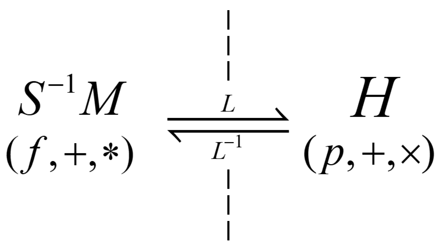
In the operational field H, the basic element p is defined as p = d/dt, which is the derivative with respect to the time variable t. The time axis is inherently defined on $(0,+\infty )$. Therefore, we use the Laplace transform as the homomorphism to characterize the relationship between the operational field and the convoluted field, and we refer to this homomorphism as the L-homomorphism.

In previous studies of operator algebra, the Laplace transform has always emerged. However, there has been no convincing explanation for why the Laplace transform is so important and indispensable. With the abstraction of operational algebra, we can now provide an answer to this question: the Laplace transform is the homomorphism from the convoluted field to the operational field. The core of the entire operator algebra lies in the homomorphic relationship between the operational field and the convoluted field. Leveraging the established algebraic system, commonly used classical concepts can now be given a more general algebraic interpretation:

The convolution kernel function is an element of the convoluted field; the operator is an element of the operational field. The inverse Laplace transform of an operator is its corresponding convolution kernel function, that is,

$$L^{-1}[T(p)]=f(t), L^{-1}:H\to S^{-1}M.$$

(26)

Thus, the final piece of the L-homomorphism in the operator algebra system is completed. The core of the entire operator algebra is now redefined as the homomorphic relationship between the operational field and the convoluted field, forming an elegant and symmetrical structure as shown in Figure 1. The ambiguities left by Mikusiński have now been fully clarified.

7. Discussion

The previous sections have constructed a concise and elegant operator algebra structure. In this section, we use the classic one-dimensional heat conduction equation as an example to reveal the correspondence between operational calculus solutions and the abstract operator algebra structure. This demonstrates that the algebraic structure established in this work is indeed the abstract formulation of the operational calculus method.

The one-dimensional heat conduction equation and boundary condition is given by

$$u_{xx}=a^2{u}_t, u(0,t)=u_0(t), \underset{x\to \infty }{\lim }u(x,t)=0.$$

(27)

According to Duhamel’s principle, the solution to a linear partial differential equation can always be expressed as the convolution of two functions. Therefore, it is desirable to express the equation in convolution form, as this would allow us to directly solve it in the convoluted field. However, most equations are given in product form rather than convolution form. In other words, their base field is the function field equipped with differentiation and ordinary multiplication, rather than the convoluted field, which consists of functions with convolution multiplication.

Although we can construct a homomorphism between these two fields, this homomorphism is complex, and solving convolution equations is not straightforward. Therefore, it is practical to introduce an intermediate field that facilitates the transition between the two fields while leveraging the characteristics of each field to gradually solve the equation. The final result can then be expressed in convolution form.

The intermediate field is exactly the Heaviside field H. During the transformation from the base field to the operational field, the dependent variable u in the governing equation is expressed as the action of an element p in the Heaviside field on the function u. Therefore, the governing equation in the Heaviside field can be written as

$$u_{xx}=a^{2}pu.$$

(28)

Based on the properties of the operational field H, we know that p is an independent variable consistent with x. Therefore, using the principles of multivariable calculus, we can treat Equation (28) as an ordinary differential equation in x with p as a parameter. This allows us to obtain a solution that includes p as a parameter.

$$u(x,p)=C_1{e}^{-ax\sqrt{p}}+C_2{e}^{ax\sqrt{p}}.$$

(29)

It is important to note that as the base field transforms into the operational field, the variable type of u changes from t to p. Consequently, the representation of the boundary conditions also undergoes a transformation in the operational field.

$$u(0,p)=u_0(p), \underset{x\to \infty }{\lim }u(x,p)=0.$$

(30)

By substituting the boundary conditions under the operational field, the solution can be determined as

$$u(x,p)=e^{-ax\sqrt{p}}{u}_0(p).$$

(31)

Obviously, in the original theoretical framework, $e^{-ax\sqrt{p}}$ is difficult to interpret. However, based on the framework presented in this work, it can be easily recognized that $e^{-ax\sqrt{p}}$ is fundamentally an element of the Heaviside field H, representing a class of exponential functions of the operator p.

The concepts related to the operational field clarify that operators are transformations; they do not provide a quantitative description of the specific form of these transformations. To address this, we rely on the convoluted field introduced in this work to determine the actual transformation and provide the final solution to the equation. We achieve this by using a homomorphism to transition between the operational field and the convoluted field. Specifically, we have established that the inverse Laplace transform is the homomorphism that maps elements from the operational field to the convoluted field. Therefore, transforming Equation (31) into the convoluted field yields the following result:

$$L^{-1}[u(x,p)]=L^{-1}[e^{-ax\sqrt{p}}{u}_0(p)]=L^{-1}(e^{-ax\sqrt{p}})\ast L^{-1}[u_0(p)].$$

(32)

After calculation, the inverse transformation of each term in Equation (22) can be written in the following form:

$$L^{-1}(e^{-ax\sqrt{p}})={\displaystyle \frac{ax}{2\sqrt{\pi }{t}^{\raisebox{1ex}{$3$}\!\left/ \!\raisebox{-1ex}{$2$}\right.}}}{e}^{-{\displaystyle \frac{a^2{x}^2}{4t}}}, L^{-1}[u(x,p)]=u(x,t), L^{-1}[u_0(p)]=u_0(t)$$

(33)

Substituting the expression from Equation (32) into the inverse Laplace transform, we obtain the well-known analytical solution to the one-dimensional heat conduction equation.

$$u(x,t)={\displaystyle \frac{ax}{2\sqrt{\pi }{t}^{\raisebox{1ex}{$3$}\!\left/ \!\raisebox{-1ex}{$2$}\right.}}}{e}^{-{\displaystyle \frac{a^2{x}^2}{4t}}}\ast u_0(t)={\displaystyle \frac{ax}{2\sqrt{\pi }}}{\displaystyle {\int }_0^t{u}_0(t-\tau )\frac{e^{-\frac{a^2{x}^2}{4\tau }}}{{\tau }^{\raisebox{1ex}{$3$}\!\left/ \!\raisebox{-1ex}{$2$}\right.}}}d\tau .$$

(34)

Compared to traditional methods for solving differential equations, the operational calculus approach is notably clearer and more concise. However, in its original form, the operational calculus method faced a significant limitation: the non-singular operator $e^{-ax\sqrt{p}}$ could not be properly interpreted. As a result, practitioners had to rely on known solutions and ad hoc methods to determine the convolution kernel function, severely restricting its applicability. Later, although general methods for computing convolution kernel functions were developed, the logical foundation of these methods remained unexplained.

In this work, by constructing a rigorous algebraic structure, we provide a solid logical foundation for every step of the operational calculus method. Furthermore, we offer a natural explanation for the solution steps from an algebraic perspective.

8. Conclusions

This work establishes a new operator algebraic foundation for operational calculus. This system abandons Mikusiński’s concept of a single operator field and instead defines two distinct algebraic structures: the operational field and the convoluted field. By establishing a homomorphism between these two algebraic structures, we provide a clear and rigorous framework for operator algebra theory, resolving the ambiguities present in the original theory. Furthermore, the new system places integral transforms at the core of operator algebra theory, constructing a logical foundation for the operator kernel function method.

Our main logical construction process is illustrated in Figure 2. The traditional operator algebra system conflates two types of operators, p and f/g, leading to a certain degree of confusion. To address this, we constructed two separate algebraic structures, each containing one of these operators. We introduced the Mikusiński function set K and defined addition and convolution operations on it, resulting in the convoluted ring M. By further performing fractionalization, we extended the ring M to the convoluted field $S^{-1}M$, ultimately unifying operators of the form f/g under the convolution field.

At the same time, we analyzed specific properties of the convoluted field $S^{-1}M$, obtaining interesting and profound conclusions. For example, the Dirac delta function δ(t) is the identity element in the convolution field, and the operator-like properties in the convoluted field arise from the interaction between elements and the convolution operation.

For the other type of operators involving p, we used an inductive approach to define the set $C^{\infty }(p)$. By introducing addition and ordinary multiplication into $C^{\infty }(p)$, we constructed the Heaviside field H, which contains operators of the form T(p). This completed the separation of the two types of operators, placing f/g operators in the convoluted field $S^{-1}M$ and T(p) operators in the Heaviside field H.

We also introduced integral transforms as homomorphisms between the two algebraic structures, enabling a quantitative description of their interactions. Finally, we demonstrated that this algebraic structure serves as the logical foundation of the operational calculus system (see Figure 2).

Operational calculus is the formalized theory of calculus. Undoubtedly, under the definition where the differential symbol is denoted as an operator p, forms such as p^1/n are all fractional-order operators. The research results of this paper provide a more rigorous logical foundation for dealing with the kernel function of fractional-order operators and presents an effective methodology for research of fractional-order effects.