Error Analysis of the L1 Scheme on a Modified Graded Mesh for a Caputo–Hadamard Fractional Diffusion Equation

Abstract

The $L1$ scheme on a modified graded mesh is proposed to solve a Caputo–Hadamard fractional diffusion equation with order $\alpha \in (0,1)$. Firstly, an improved graded mesh frame is innovatively constructed, and its mathematical properties are verified. Subsequently, a new truncation error bound for the L1 discretisation format of Caputo–Hadamard fractional-order derivatives is established by means of a Taylor cosine expansion of the integral form, and a second-order central difference method is used to achieve high-precision discretisation of spatial derivatives. Furthermore, a rigorous analysis of stability and convergence under the maximum norm is conducted, with special attention devoted to validating that the $L1$ approximation scheme manifests an optimal convergence order of $2-\alpha$ when deployed on the modified graded mesh. Finally, the theoretical results are substantiated through a series of numerical experiments, which validate their accuracy and applicability.

1. Introduction

It is well known that Caputo time-fractional differential equations have broad applications in modeling complex systems with memory effects and non-local dynamics (see [1,2,3], for example). While significant progress has been made in both mathematical analysis [4,5] and numerical methods [6,7,8,9] for Caputo fractional derivatives, the construction of theoretical foundations for Caputo–Hadamard operators is still relatively lagging behind, and both early explorations [10,11,12,13] and recent progress [14,15,16] indicate the slow pace of development in this direction. In general, closed-form analytical solutions for Caputo–Hadamard fractional differential equations remain elusive. Even when such solutions can be theoretically derived, their practical computation becomes highly problematic due to the inherent complexity introduced by the specialized functions required for their construction. The non-elementary nature of these solutions not only complicates numerical evaluation but also limits their applicability in real-world scenarios, where computational efficiency and algorithmic implementability are critical considerations. This fundamental challenge underscores the necessity for developing alternative approximation strategies that balance analytical rigor with computational feasibility.

The field of numerical methods for Hadamard fractional-order differential Equations (HFDEs) has experienced significant advancements in recent years, driven by the theoretical interests and practical demands in modeling complex systems with memory-dependent behaviors. For instance, the authors in [17,18] developed spectral collocation methods for solving Caputo–Hadamard fractional-order differential equations. He, et al., in Ref. [19], proposed a region decomposition algorithm for Caputo–Hadamard fractional-order differential equations. In view of the non-locality of the fractional-order derivatives, the fractional operator is decomposed into historical and local components with a local time integrator compressed by a Gauss–Jacobi kernel. Gohar, et al. [20] proposed a finite difference method on a uniform mesh for an initial value problem (IVP) with a Caputo–Hadamard derivative. It is noted that the analytical solutions of time-fractional differential equations with a Caputo–Hadamard fractional derivative are characterized by a distinctive feature known as the weak singularity formation near the temporal origin $(t\to 1^{+})$. The emergence of weak singularities imposes significant challenges on the construction of numerical schemes. Therefore, these specialized nonuniform discretization meshes (see [21,22,23,24], for example) are designed to concentrate computational resources in the vicinity of the singularity $(t\to 1^{+})$. Among these presented nonuniform meshes, the graded mesh (G-mesh) emerges as the most widely adopted framework for resolving weak singularities. The mathematical formulation of a typical G-mesh can be expressed as follows:

$$\begin{array}{c}\hfill t_n=a{\left({\displaystyle \frac{T}{a}}\right)}^{{\left({\displaystyle \frac{n}{N}}\right)}^r},r\ge 1,0\le n\le N,\end{array}$$

(1)

where $r\ge 1$ and $a\ge 1$ is a mesh grading constant and N is a mesh parameter.

Recently, Liu, et al. [25] constructed a finite difference scheme on a modified graded mesh for a time-fractional diffusion equation with a Caputo fractional derivative. It should be pointed out that the proposed modified graded mesh is strategically designed to combine localized refinement near the initial temporal boundary $(t=0)$ with uniform discretization in subsequent temporal domains; thereby, the error will be smaller while maintaining the accuracy of the solution. Extending the error analysis methodology developed in [25], we introduce a modified graded mesh formulation to establish a novel numerical scheme for the Caputo–Hadamard fractional diffusion equation defined as follows:

$$\left\{\begin{array}{cc}\hfill & {}_{\mathit{CH}}D_{a,t}^{\alpha }u(x,t)-{\displaystyle \frac{{\partial }^{2}u(x,t)}{\partial x^2}}=f(x,t),(x,t)\in \mathcal{Q},\hfill \\ \hfill & u(x,a)=\varphi \left(x\right),x\in \overline{\Omega }=\Omega \cup \partial \Omega ,\mathrm{if}\alpha \in (0,1),\hfill \\ \hfill & u(0,t)=u(L,t)=0,t\in (a,T],\hfill \end{array}\right.$$

(2)

where $\Omega =(0,L)$, $\partial \Omega$ is the boundary of $\Omega$, $\mathcal{Q}:=(0,L)\times (a,T]$ and $f(x,t)$, $\varphi \left(x\right)$ are given functions. Furthermore, we assume the compatibility condition $\varphi \left(0\right)=\varphi \left(L\right)=0$ holds. The symbol ${}_{\mathit{CH}}D_{a,t}^{\alpha }$ is the Caputo–Hadamard derivative with order $\alpha$ as follows:

$${}_{\mathit{CH}}D_{a,t}^{\alpha }u(x,t)={\int }_a^t{\omega }_{1-\alpha }(\log t-\log s)\delta u(x,s){\displaystyle \frac{ds}{s}},0<a<t,$$

(3)

where ${\omega }_{\beta }\left(t\right):={\displaystyle \frac{t^{\beta -1}}{\Gamma \left(\beta \right)}},\delta u(x,s)=\left(s{\displaystyle \frac{\partial }{\partial s}}\right)u(x,s),0<\alpha <1$. In this paper, the log is defined as the logarithm with base e.

The contribution of this paper is constructing a new nonuniform mesh and calling it the modified graded mesh. Under this presented mesh, we use the $L1$ formula to approximate the time fractional-order derivatives of problem (2), which lead to a convergence rate of $2-\alpha$ in the time direction. The proposed method in this paper is analyzed under the following regularity assumptions [21]:

$$\begin{array}{c}\hfill \left|{\displaystyle \frac{{\partial }^{k}u(x,t)}{\partial x^k}}\right|\le C,k=0,1,2,3,4,\end{array}$$

(4)

$$\begin{array}{c}\hfill \left|{\delta }^{k}u(x,t)\right|\le C\left(1+{\left(\log {\displaystyle \frac{t}{a}}\right)}^{\alpha -k}\right),k=0,1,2,3,\end{array}$$

(5)

for all $(x,t)\in [0,L]\times (a,T]$, and C is a positive constant. Throughout this paper, the generic constant C is a positive constant and may take different values at different places.

The layout of the paper is as follows: Section 2 introduces and analyzes a modified graded mesh (MG-mesh). Section 3 scrutinizes the stability and convergence of the discrete scheme by means of a paradigm analysis. The main results, in particular, the truncation error and convergence, are then studied in depth in Section 4. Numerical examples are given in Section 5 to demonstrate the validity of the theoretical results. Finally, Section 6 draws some conclusions.

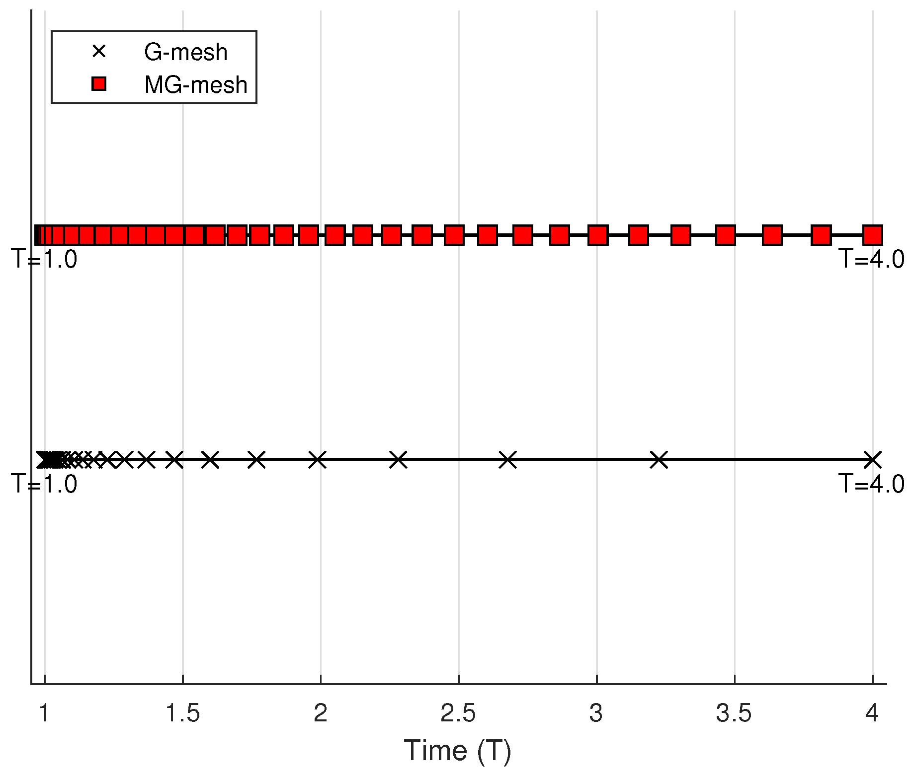
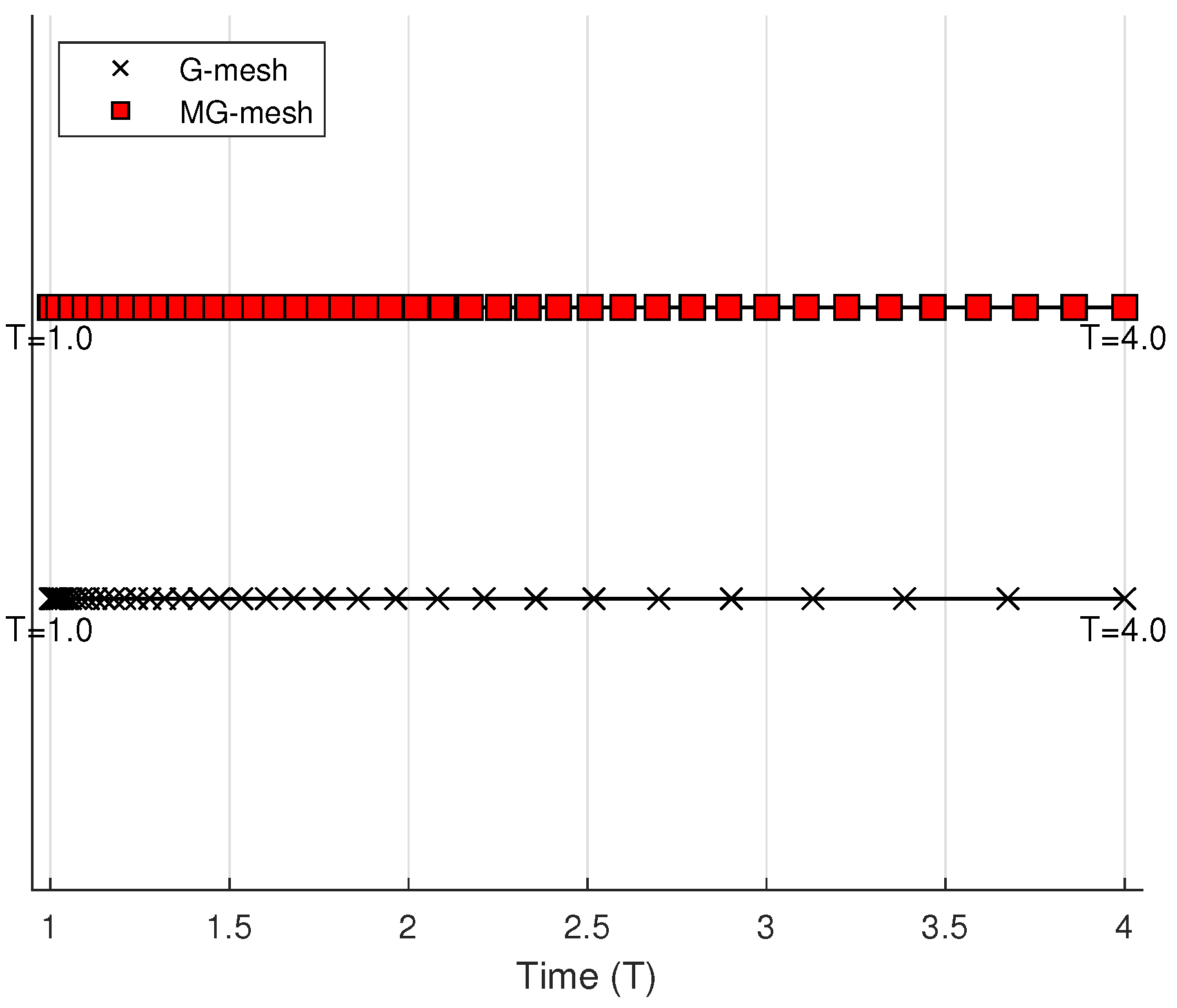
2. A Modified Graded Mesh

Let ${\overline{\Omega }}^N=\left\{a=t_0<t_1<\cdots <t_N=T\right\}$ be an arbitrary nonuniform mesh with N subintervals on $[a,T]$, which satisfies the following mesh equidistribution principle

$${\int }_{t_n}^{t_{n+1}}\tilde{M}\left(s\right){\displaystyle \frac{ds}{s}}={\displaystyle \frac{1}{N}}{\int }_a^T\tilde{M}\left(s\right){\displaystyle \frac{ds}{s}},\mathrm{for}n=0,1,\dots ,N-1,$$

(6)

where $\tilde{M}\left(s\right)$ is a given positive monitor function. In order to obtain this ${\left\{t_n\right\}}_{n=0}^N$, we choose the monitor function $\tilde{M}\left(t\right)$ as follows:

$$\tilde{M}\left(t\right)=max\left\{\log T,K{\left(\log t\right)}^{{\displaystyle \frac{\alpha }{2}}-1}\right\},$$

(7)

where $K\in (0,\log T]$ is a user-chosen constant. Here, we call it the modified graded mesh. Obviously, let $\sigma =e^{{\left({\displaystyle \frac{\log T}{K}}\right)}^{{\displaystyle \frac{2}{\alpha -2}}}}$, and with the choice of this constant K, there exists a subinterval $I:=[\sigma ,T]$ such that

$$\log a<K{\left(\log t\right)}^{{\displaystyle \frac{\alpha }{2}}-1}\le \log T,\forall t\in I.$$

Let J be the index such that $t_{J-1}<\sigma \le t_J$. By simple calculation, our presented modified graded mesh ${\left\{t_n\right\}}_{n=0}^N$ can be obtained by

$$t_n=\left\{\begin{array}{ccc}\hfill & e^{{\left({\displaystyle \frac{\alpha P}{2K}}\right)}^{{\displaystyle \frac{2}{\alpha }}}{\left({\displaystyle \frac{n}{N}}\right)}^{{\displaystyle \frac{2}{\alpha }}}},\hfill & \hfill n=0,\cdots ,J-1,\\ \hfill & e^{\left(1-{\displaystyle \frac{2}{\alpha }}\right)g+{\displaystyle \frac{Pn}{N\log T}}},\hfill & \hfill n=J,J+1,\cdots ,N,\end{array}\right.$$

(8)

where

$$P={\int }_a^T\tilde{M}\left(s\right){\displaystyle \frac{ds}{s}}={\displaystyle \frac{2K}{\alpha }}g+\log T(\log T-g)$$

and

$$g={\left({\displaystyle \frac{\log T}{K}}\right)}^{{\displaystyle \frac{2}{\alpha -2}}}.$$

Obviously, when $\log T\ge 1$, we have $P/\log T>1$.

As mentioned above, Equation (8) mathematically describes the time modified graded mesh in this paper. The MG-mesh is divided into the following two distinct parts within the time interval $[a,T]$: For indices $n=0,\cdots ,J-1$, a nonuniform discretization is adopted, whereas for $n=J,J+1,\cdots ,N$, a uniform grid is utilized. Figure 1 illustrates the time distribution of the MG-mesh compared to the conventional G-mesh (where $r=2/\alpha$) for the parameters $N=40,a=1,T=4$, and $\alpha =0.3$. Figure 2 shows the $\alpha$ in Figure 1 is taken as 0.8 and the rest is kept constant. It can be clearly observed from the figure that the MG-mesh (8) contains more grid points than the conventional G-mesh (1) as time grows, a property that helps to reduce computational errors.

Lemma 1.

Let ${\left\{t_n\right\}}_{n=0}^N$ be the modified graded mesh defined in (8) and ${\tau }_n:=\log t_n-\log t_{n-1}$ for $n=1,\dots ,N$. Then,

$${\tau }_n\le C{N}^{-1},n=1,\dots ,N.$$

(9)

In addition, the exact solution $u(x,t)$ of problem (2) satisfies

$${\int }_{t_n}^{t_{n+1}}\left|{\displaystyle \frac{{\partial }^{2}u}{\partial t^2}}(x,t)\right|\left(\log {\displaystyle \frac{t}{t_n}}\right){\displaystyle \frac{dt}{t}}\le C{N}^{-2},n=0,\dots ,N-1,x\in [0,l].$$

(10)

Proof. 

For $n=1,\dots ,N$, it follows from Equations (6) and (7) that

$$\begin{array}{cc}\hfill {\tau }_n& ={\displaystyle \frac{1}{\log T}}{\int }_{t_{n-1}}^{t_n}\log T{\displaystyle \frac{dt}{t}}\le {\displaystyle \frac{1}{\log T}}{\int }_{t_{n-1}}^{t_n}\tilde{M}\left(t\right){\displaystyle \frac{dt}{t}}\hfill \\ \hfill & ={\displaystyle \frac{1}{N\log T}}{\int }_a^T\tilde{M}\left(t\right){\displaystyle \frac{dt}{t}}\hfill \\ \hfill & ={\displaystyle \frac{P}{N\log T}}=C{N}^{-1},\hfill \end{array}$$

(11)

which completes the proof of (9). Furthermore, from (5) and (11), we have

$$\begin{array}{cc}\hfill {\int }_{t_n}^{t_{n+1}}\left|{\displaystyle \frac{{\partial }^{2}u}{\partial t^2}}(x,t)\right|\left(\log {\displaystyle \frac{t}{t_n}}\right){\displaystyle \frac{dt}{t}}& \le C{\int }_{t_n}^{t_{n+1}}{\left(\log t\right)}^{\alpha -2}\left(\log {\displaystyle \frac{t}{t_n}}\right){\displaystyle \frac{dt}{t}}+C{\int }_{t_n}^{t_{n+1}}\left(\log {\displaystyle \frac{t}{t_n}}\right){\displaystyle \frac{dt}{t}}\hfill \\ \hfill & \le C{\left[{\int }_{t_n}^{t_{n+1}}{\left(\log t\right)}^{{\displaystyle \frac{\alpha }{2}}-1}{\displaystyle \frac{dt}{t}}\right]}^2+C{\tau }_n^2\hfill \\ \hfill & \le C{\left[{\int }_{t_n}^{t_{n+1}}\tilde{M}\left(t\right){\displaystyle \frac{dt}{t}}\right]}^2+C{\tau }_n^2\hfill \\ \hfill & =C{N}^{-2},\hfill \end{array}$$

(12)

where we have used the estimation (9) and the fact that

$${\int }_a^b\varphi \left(t\right)(t-a)dt\le {\displaystyle \frac{1}{2}}{\left({\int }_a^b\sqrt{\varphi \left(t\right)}dt\right)}^2$$

holds true for any positive monotonically decreasing function $\varphi \left(t\right)$ on $[a,b]$. The proof is completed. □

Lemma 2.

For $n=1,\dots ,N$,

$$t_n\le e^{{\displaystyle \frac{Pn}{N\log T}}},n=J,J+1,\dots ,N,$$

(13)

$$C{N}^{-{\displaystyle \frac{2}{\alpha }}}{\left(n\right)}^{{\displaystyle \frac{2}{\alpha }}-1}\le {\tau }_{n+1}\le C{N}^{-{\displaystyle \frac{2}{\alpha }}}{(n+1)}^{{\displaystyle \frac{2}{\alpha }}-1},n=1,\cdots ,J-2.$$

(14)

Proof. 

Obviously, it follows from the second equation of (8) that

$$t_n=e^{\left(1-{\displaystyle \frac{2}{\alpha }}\right)\sigma +{\displaystyle \frac{Pn}{N\log T}}}\le e^{{\displaystyle \frac{Pn}{N\log T}}}\mathrm{for}\alpha \in (0,1)\mathrm{and}n=J,J+1,\dots ,N.$$

In addition, since ${\tau }_{n+1}=\log \left(t_{n+1}\right)-\log \left(t_n\right)=w_{n+1}^{{\displaystyle \frac{2}{\alpha }}}-w_n^{{\displaystyle \frac{2}{\alpha }}}$, where $w_n={\displaystyle \frac{\alpha Pi}{2Nn}}$, it is easy to show from the mean value theorem that

$${\tau }_{n+1}={\displaystyle \frac{2}{\alpha }}{\xi }_n^{{\displaystyle \frac{2}{\alpha }}-1}{N}^{-{\displaystyle \frac{2}{\alpha }}},{\xi }_n\in (w_n,w_{n+1}),n=1,\cdots ,J-2.$$

(15)

Thus, the desired results of (14) can be followed from (15). □

3. Discretization Scheme

In this section, we shall construct a finite difference scheme on a mesh $(x_i,t_n)(i=0,1,\cdots ,M,n=0,1,\cdots ,N)$ for problem (2), where $x_i=ih$ is a uniform mesh with the mesh step $h={\displaystyle \frac{l}{M}}$ and ${\left\{t_n\right\}}_{n=0}^N$ is the modified mesh defined in (8). Correspondingly, we also denote ${\tau }_n:=\log t_n-\log t_{n-1}$.

For a given mesh function $u={\left\{u_i\right\}}_{i=0}^M$, define the following difference operators

$${\delta }_x{u}_{i-{\displaystyle \frac{1}{2}}}={\displaystyle \frac{u_i-v_{i-1}}{h}},{\delta }_x^2{u}_i={\displaystyle \frac{u_{i+1}-2u_i+u_{i-1}}{h^2}}.$$

Meanwhile, for the Caputo–Hadamard derivative $\left({}_{\mathit{CH}}D_{a,t}^{\alpha }u\right)\left(t_n\right)$, by using the approximation method given in [20], we have

$${\left.{}_{\mathit{CH}}D_{a,t}^{\alpha }u\left(t\right)\right|}_{t=t_n}={\displaystyle \frac{1}{\Gamma (2-\alpha )}}\sum _{j=0}^{n-1}{d}_{n,j}\left(u\left(t_{j+1}\right)-u\left(t_j\right)\right)+{{\rm Y}}^n,$$

(16)

where

$$d_{n,j}={\displaystyle \frac{{\left(\log \frac{t_n}{t_{n-j}}\right)}^{1-\alpha }-{\left(\log \frac{t_n}{t_{n-j+1}}\right)}^{1-\alpha }}{\log \frac{t_{n-j+1}}{t_{n-j}}}},j=1,2,\dots ,n,$$

(17)

and ${{\rm Y}}^n$ is the truncation error, which is given by

$${{\rm Y}}^n={\displaystyle \frac{1}{\Gamma (1-\alpha )}}\sum _{j=0}^{n-1}{\int }_{t_j}^{t_{j+1}}{\left(\log {\displaystyle \frac{t_n}{s}}\right)}^{-\alpha }\left(\delta u\left(s\right)-{\displaystyle \frac{u\left(t_{j+1}\right)-u\left(t_j\right)}{\log \frac{t_{j+1}}{t_j}}}\right){\displaystyle \frac{ds}{s}}.$$

(18)

Thus, we obtain the discretization scheme of (2) as follows:

$$\begin{array}{cc}\hfill & {\displaystyle \frac{1}{\Gamma (2-\alpha )}}\sum _{j=0}^{n-1}{d}_{n,j}\left(u_i^{j+1}-u_i^j\right)-{\delta }_x^2{u}_i^n=f_i^n,\hfill \\ \hfill & u_i^0=\varphi \left(x_i\right),0\le i\le M,\hfill \\ \hfill & u_0^n=u_M^n=0,1\le n\le N.\hfill \end{array}$$

(19)

Let ${\mathcal{U}}_{\infty }=\left\{u\mid u=(u_0,u_1,\dots ,u_N),u_0=u_N=0\right\}$. For any $u\in {\mathcal{U}}_{\infty }$, the following discrete inner product and the corresponding norm will be used:

$$\begin{array}{cc}\hfill {\delta }_x{u}_{j-{\displaystyle \frac{1}{2}}}^n& ={\displaystyle \frac{1}{h}}(u_j^n-u_{j-1}^n),\hfill \\ \hfill {\delta }_x^2{u}_j^n& ={\displaystyle \frac{1}{h^2}}(u_{j-1}^n-2u_j^n+u_{j+1}^n),\hfill \\ \hfill \parallel u\parallel & =\sqrt{(u,u)}.\hfill \end{array}$$

Furthermore, we define the real numbers ${\theta }_{n,m}$ for $n=1,\dots ,N$ and $m=1,\dots ,n-1$ as

$${\theta }_{n,n}=1,{\theta }_{n,m}=\sum _{k=1}^{n-m}{\tau }_{n-k}^{\alpha }\left(d_{n,k}-d_{n,k+1}\right){\theta }_{n-k,m}.$$

(20)

Similar to the argument of Lemma 3.1 of [25], we can obtain the following results.

Lemma 3.

Let the parameter $\beta \le 2$. Then, for $n=1,\dots ,N$, we have

$${\tau }_n^{\alpha }\sum _{m=1}^n{m}^{-\beta }{\theta }_{n,m}\le {\chi }_1{N}^{-\beta },n=1,\dots ,J-1,$$

(21)

$${\tau }_n^{\alpha }\sum _{m=1}^n{\theta }_{n,m}\le {\chi }_2,J\le n\le N,$$

(22)

where ${\chi }_1={\displaystyle \frac{1}{1-\alpha }}{\left({\displaystyle \frac{\alpha P}{2K}}\right)}^2,{\chi }_2={\displaystyle \frac{1}{1-\alpha }}{\left({\displaystyle \frac{P}{K}}\right)}^2$.

Proof. 

The proof of (21) is similar to Lemma 4.3 in [26].

Next, to derive (22), we first study the case for $n=J$. Let $\beta =0$. It follows from (21) that

$${\tau }_n^{\alpha }\sum _{m=1}^n{\theta }_{n,m}\le {\chi }_1\le {\chi }_2,n=1,\dots ,J-1.$$

Furthermore,

$$\begin{array}{cc}\hfill {\tau }_J^{\alpha }\sum _{m=1}^J{\theta }_{J,m}& ={\tau }_J^{\alpha }{\theta }_{J,J}+{\tau }_J^{\alpha }\sum _{m=1}^{J-1}\sum _{j=1}^{J-m}{\tau }_{J-j}^{\alpha }\left(d_{J,j}-d_{J,j+1}\right){\theta }_{J-j,m}\hfill \\ \hfill & ={\tau }_J^{\alpha }+{\tau }_J^{\alpha }\sum _{j=1}^{J-1}(d_{J,j}-d_{J,j+1}){\tau }_{J-j}^{\alpha }\sum _{m=1}^{J-j}{\theta }_{J-j,m}\hfill \\ \hfill & \le {\tau }_J^{\alpha }+{\tau }_J^{\alpha }\sum _{j=1}^{J-1}(d_{J,j}-d_{J,j+1}){\chi }_2\hfill \\ \hfill & ={\tau }_J^{\alpha }+{\tau }_J^{\alpha }(d_{J,1}-d_{J,J}){\chi }_2\hfill \\ \hfill & ={\chi }_2+{\tau }_J^{\alpha }\left(1-d_{J,J}{\chi }_2\right).\hfill \end{array}$$

(23)

The next thing to do in the proof is $d_{J,J}{\chi }_2\ge 1$. By calculation, we have

$$\begin{array}{cc}\hfill d_{J,J}{\chi }_2& ={\displaystyle \frac{{\left(\log t_J\right)}^{1-\alpha }-{\left(\log t_J-\log t_1\right)}^{1-\alpha }}{{\tau }_1}}{\chi }_2\hfill \\ \hfill & \ge (1-\alpha ){\left(\log t_J\right)}^{-\alpha }{\chi }_2\hfill \\ \hfill & ={\left({\displaystyle \frac{\log T}{P}}\right)}^{-\alpha }{\left({\displaystyle \frac{P}{K}}\right)}^2{\left({\displaystyle \frac{N}{J}}\right)}^{\alpha }\hfill \\ \hfill & ={\left({\displaystyle \frac{P}{\log T}}\right)}^{2-\alpha }{\left({\displaystyle \frac{\log T}{K}}\right)}^2{\left({\displaystyle \frac{N}{J}}\right)}^{\alpha }\hfill \\ \hfill & \ge 1,\hfill \end{array}$$

(24)

where we have used the mean value theorem and (13), $P>\log T$, and $K<\log T$. Similarly, (22) holds true for $n=J+1,\dots ,N$. The proof of this Lemma is completed. □

Lemma 4

([21]). For $0<\alpha <1$, the coefficients $d_{n,j}$ ($1\le j\le n,1\le n\le N$) in (18) satisfy the following:

$$d_{n,1}>d_{n,2}>\cdots >d_{n,j}>d_{n,j+1}>\cdots >d_{n,n}>0,$$

and the bounds for $d_{n,j}$ are given by the following:

$$(1-\alpha ){\left(\log {\displaystyle \frac{t_n}{t_{n-j}}}\right)}^{-\alpha }\le d_{n,j}\le (1-\alpha ){\left(\log {\displaystyle \frac{t_n}{t_{n-j+1}}}\right)}^{-\alpha }.$$

Finally, let $u^n={(u_0^n,u_1^n,\dots ,u_M^n)}^T$, $f={(f(x_0,t_n),f(x_i,t_n),\dots ,f(x_M,t_n))}^T$. Then, similar to the argument of Lemma 4.2 given in [26], we give the stability for the discretization scheme (19).

Theorem 1.

Let $u^n$ with $1\le n\le N$ be the solution of the difference scheme (19). Then, we have

$$\parallel u^n{\parallel }_{\infty }\le \parallel u^0{\parallel }_{\infty }+{\tau }_n^{\alpha }\Gamma (2-\alpha )\sum _{j=1}^n{\theta }_{n,j}{\parallel f^j\parallel }_{\infty }$$

4. Error Analysis

For a given i, $i=1,2,\dots ,M-1$, and $n=1,2,\dots ,N$, let

$${{\rm Y}}^n:=\left({}_{\mathrm{CH}}D_{a,t}^{\alpha }u\right)\left(t_n\right)-{\left({}_{\mathrm{CH}}D_{a,t}^{\alpha }u\right)}^n=\sum _{j=1}^n{r}_{n,j}$$

(25)

denote the truncation error at time knot $t_n$, where

$$r_{n,j}={\displaystyle \frac{1}{\Gamma (1-\alpha )}}{\int }_{s=t_j}^{t_{j+1}}{\left(\log {\displaystyle \frac{t_n}{s}}\right)}^{-\alpha }\left[{\displaystyle \frac{u\left(x_i,t_{j+1}\right)-u\left(x_i,t_j\right)}{{\tau }_{j+1}}}-{\displaystyle \frac{\partial u\left(x_i,s\right)}{\partial s}}\right]{\displaystyle \frac{ds}{s}}.$$

(26)

Lemma 5.

For $i=1,\dots ,M-1$, and $n=1,\dots ,N$,

$$\left|r_{n,j}\right|\le \left\{\begin{array}{c}C{\int }_{t_j}^{t_{j+1}}\left|{\displaystyle \frac{{\partial }^{2}u\left(x_i,t\right)}{\partial t^2}}\right|\left(\log {\displaystyle \frac{t}{t_j}}\right){\displaystyle \frac{dt}{t}}{\int }_{{\gamma }_j}^{{\xi }_j}{\left(\log {\displaystyle \frac{t_n}{s}}\right)}^{-\alpha -1}{\displaystyle \frac{ds}{s}},0\le j<n,n>1,\hfill \\ C{\tau }_j^{2-\alpha }\underset{t\in \left[t_j,t_{j+1}\right]}{max}\left|{\displaystyle \frac{{\partial }^{2}u\left(x_i,t\right)}{\partial t^2}}\right|,j=n-1,n=1,\dots ,N,\hfill \end{array}\right.$$

(27)

where ${\xi }_j\in (t_j,t),t\in (t_j,t_{j+1})$,${\gamma }_j\in (t_j,t_{j+1})$.

Proof. 

For $s\in (t_j,t_{j+1})$, using the Taylor series expansion, one has

$$\begin{array}{cc}\hfill & {\displaystyle \frac{u(x_i,t_{j+1})-u(x_i,t_j)}{{\tau }_{j+1}}}-{\displaystyle \frac{\partial u(x,s)}{\partial s}}\hfill \\ \hfill & ={\int }_s^{t_{j+1}}{\displaystyle \frac{{\partial }^{2}u(x_i,t)}{\partial t^2}}{\displaystyle \frac{dt}{t}}-{\displaystyle \frac{1}{{\tau }_{j+1}}}{\int }_{t_j}^{t_{j+1}}{\displaystyle \frac{{\partial }^{2}u(x_i,t)}{\partial t^2}}\left(\log {\displaystyle \frac{t}{t_j}}\right){\displaystyle \frac{dt}{t}}.\hfill \end{array}$$

(28)

Then, it follows from (26) and (28) that

$$\begin{array}{cc}\hfill & r_{n,j}={\displaystyle \frac{1}{\Gamma (1-\alpha )}}{\int }_{s=t_j}^{t_{j+1}}{\left(\log {\displaystyle \frac{t_n}{s}}\right)}^{-\alpha }{\int }_s^{t_{j+1}}{\displaystyle \frac{{\partial }^{2}u\left(x_i,t\right)}{\partial t^2}}{\displaystyle \frac{dt}{t}}{\displaystyle \frac{ds}{s}}\hfill \\ \hfill & -{\displaystyle \frac{1}{\Gamma (1-\alpha )}}{\displaystyle \frac{1}{{\tau }_{j+1}}}{\int }_{t_j}^{t_{j+1}}{\left(\log {\displaystyle \frac{t_n}{s}}\right)}^{-\alpha }{\displaystyle \frac{ds}{s}}{\int }_{t_j}^{t_{j+1}}{\displaystyle \frac{{\partial }^{2}u\left(x_i,t\right)}{\partial t^2}}\left(\log {\displaystyle \frac{t}{t_j}}\right){\displaystyle \frac{dt}{t}}.\hfill \end{array}$$

(29)

For $0\le j<n-1$ and $n>1$, exchanging the order of integration of (29) gives

$$\begin{array}{cc}\hfill r_{n,j}=& {\displaystyle \frac{1}{\Gamma (1-\alpha )}}{\int }_{t_j}^{t_{j+1}}{\int }_{t_j}^t{\left(\log {\displaystyle \frac{t_n}{s}}\right)}^{-\alpha }{\displaystyle \frac{ds}{s}}{\displaystyle \frac{{\partial }^{2}u\left(x_i,t\right)}{\partial t^2}}{\displaystyle \frac{dt}{t}}\hfill \\ \hfill -& {\displaystyle \frac{1}{\Gamma (1-\alpha )}}{\displaystyle \frac{1}{{\tau }_{j+1}}}{\int }_{t_j}^{t_{j+1}}{\left(\log {\displaystyle \frac{t_n}{s}}\right)}^{-\alpha }{\displaystyle \frac{ds}{s}}{\int }_{t_j}^{t_{j+1}}{\displaystyle \frac{{\partial }^{2}u\left(x_i,t\right)}{\partial t^2}}\left(\log {\displaystyle \frac{t}{t_j}}\right){\displaystyle \frac{dt}{t}}\hfill \\ \hfill =& {\displaystyle \frac{1}{\Gamma (1-\alpha )}}{\left(\log {\displaystyle \frac{t_n}{{\xi }_j}}\right)}^{-\alpha }{\int }_{t_j}^{t_{j+1}}{\displaystyle \frac{{\partial }^{2}u\left(x_i,t\right)}{\partial t^2}}\left(\log {\displaystyle \frac{t}{t_j}}\right){\displaystyle \frac{dt}{t}}\hfill \\ \hfill -& {\displaystyle \frac{1}{\Gamma (1-\alpha )}}{\left(\log {\displaystyle \frac{t_n}{{\gamma }_j}}\right)}^{-\alpha }{\int }_{t_j}^{t_{j+1}}{\displaystyle \frac{{\partial }^{2}u\left(x_i,t\right)}{\partial t^2}}\left(\log {\displaystyle \frac{t}{t_j}}\right){\displaystyle \frac{dt}{t}}\hfill \\ \hfill =& {\displaystyle \frac{1}{\Gamma (1-\alpha )}}{\int }_{t_j}^{t_{j+1}}{\displaystyle \frac{{\partial }^{2}u\left(x_i,t\right)}{\partial t^2}}\left(\log {\displaystyle \frac{t}{t_j}}\right){\displaystyle \frac{dt}{t}}\left[{\left(\log {\displaystyle \frac{t_n}{{\xi }_j}}\right)}^{-\alpha }-{\left(\log {\displaystyle \frac{t_n}{{\gamma }_j}}\right)}^{-\alpha }\right]\hfill \\ \hfill =& {\displaystyle \frac{1}{\Gamma (1-\alpha )}}{\int }_{t_j}^{t_{j+1}}{\displaystyle \frac{{\partial }^{2}u\left(x_i,t\right)}{\partial t^2}}\left(\log {\displaystyle \frac{t}{t_j}}\right){\displaystyle \frac{dt}{t}}{\int }_{{\gamma }_j}^{{\xi }_j}{\displaystyle \frac{1}{1-\alpha }}{\left(\log {\displaystyle \frac{t_n}{s}}\right)}^{-\alpha -1}\left(-{\displaystyle \frac{1}{s}}\right)ds\hfill \\ \hfill =& -{\displaystyle \frac{1}{\Gamma (2-\alpha )}}{\int }_{t_j}^{t_{j+1}}{\displaystyle \frac{{\partial }^{2}u\left(x_i,t\right)}{\partial t^2}}\left(\log {\displaystyle \frac{t}{t_j}}\right){\displaystyle \frac{dt}{t}}{\int }_{{\gamma }_j}^{{\xi }_j}{\left(\log {\displaystyle \frac{t_n}{s}}\right)}^{-\alpha -1}{\displaystyle \frac{ds}{s}},\hfill \end{array}$$

(30)

where the mean value theorem has been used and ${\xi }_j\in (t_j,t),t\in (t_j,t_{j+1})$,${\gamma }_j\in (t_j,t_{j+1})$.

Furthermore, we have

$$\left|r_{n,j}\right|\le C{\int }_{t_j}^{t_{j+1}}\left|{\displaystyle \frac{{\partial }^{2}u\left(x_i,t\right)}{\partial t^2}}\right|\left(\log {\displaystyle \frac{t}{t_j}}\right){\displaystyle \frac{dt}{t}}{\int }_{s=t_j}^{t_{j+1}}{\left(\log {\displaystyle \frac{t_n}{s}}\right)}^{-\alpha -1}{\displaystyle \frac{ds}{s}},$$

(31)

which completes the proof of the first case of (27).

Next, for $j=n-1$ and $n=1,\dots ,N$, using (26), one has

$$\begin{array}{cc}\hfill \left|r_{n,n}\right|& \le {\displaystyle \frac{1}{\Gamma (1-\alpha )}}{\int }_{t_{n-1}}^{t_n}{\left(\log {\displaystyle \frac{t_n}{s}}\right)}^{-\alpha }\left|{\displaystyle \frac{\partial u}{\partial s}}\left(x_i,{\gamma }_n\right)-{\displaystyle \frac{\partial u}{\partial s}}\left(x_i,s\right)\right|{\displaystyle \frac{ds}{s}}\hfill \\ \hfill & \le C{\tau }_n^{2-\alpha }\underset{t\in [t_j,t_{j+1}]}{max}\left|{\displaystyle \frac{{\partial }^{2}u\left(x_i,t\right)}{\partial t^2}}\right|,\hfill \end{array}$$

(32)

where the mean value theorem has been used and ${\gamma }_n\in \left(t_{n-1},t_n\right)$. This completes the proof of the second case of (27). □

Based on Lemma 5, it is easy to obtain the following result:

Corollary 1.

For $i=1,\dots ,M-1$, and $n=1,\dots ,N$, we have

$$\begin{array}{cc}\hfill & \left|r_{n,j}\right|\le C{\tau }_{j+1}^2\underset{t\in [t_j,t_{j+1}]}{max}\left|{\displaystyle \frac{{\partial }^{2}u\left(x_i,t\right)}{\partial t^2}}\right|{\int }_{t_j}^{t_{j+1}}{\left(\log {\displaystyle \frac{t_n}{s}}\right)}^{-\alpha -1}{\displaystyle \frac{ds}{s}},0\le j<n-1,n\ne 1\hfill \end{array}$$

and

$$\begin{array}{cc}\hfill & \left|r_{n,j}\right|\le C{\tau }_{j+1}^{2-\alpha }\underset{t\in [t_j,t_{j+1}]}{max}\left|{\displaystyle \frac{{\partial }^{2}u\left(x_i,t\right)}{\partial t^2}}\right|,j=n-1,n=1,\dots ,N.\hfill \end{array}$$

Remark 1.

Obviously, it is shown from Lemma 5 that our new truncation error bounds given in (27) for $\left|r_{n,j}\right|$ are much lower than those given in [21].

Lemma 6.

For a given mesh ${\left\{t_n\right\}}_{n=0}^N$ defined in (8), there exists a constant C such that

$$\left|{{\rm Y}}^n\right|\le \left\{\begin{array}{cc}C{n}^{-(2-\alpha )}\hfill & forn=1,\dots ,J-1,\hfill \\ C{N}^{-(2-\alpha )}\hfill & forn=J,\dots ,N.\hfill \end{array}\right.$$

(33)

Proof. 

In order to prove this Lemma, we study the following three cases:

1.

When $n\le J$. In this case, we should study the estimations of ${\displaystyle \sum _{j=1}^{n-2}}\left|r_{n,j}\right|$ for $2<n\le J-1$, $\left|r_{n,n-1}\right|$ for $1<n\le J-1$, $\left|r_{J,J-1}\right|$, respectively.

2.

When $N\ge n>J$. In this case, we will also give the estimations of ${\displaystyle \sum _{j=1}^{n-2}}\left|r_{n,j-1}\right|$$(J<n\le N)$ and $\left|r_{n,n-1}\right|$$(J<n<N)$.

3.

When $j=0$. In this case, we mainly discuss the bounds of $r_{n,0}$ for $1\le n<J$ and $r_{n,0}$ for $n\ge J$.

Case 1. At first, for $2<n\le J-1$, from Lemma 1 and (25), we have

$$\begin{array}{cc}\hfill \sum _{j=1}^{n-2}\left|r_{n,j}\right|& \le C\sum _{j=1}^{n-2}{\int }_{t_j}^{t_{j+1}}\left|{\displaystyle \frac{{\partial }^{2}u\left(x_i,t\right)}{\partial t^2}}\right|\left(\log {\displaystyle \frac{t}{t_j}}\right){\displaystyle \frac{dt}{t}}{\int }_{t_j}^{t_{j+1}}{\left(\log {\displaystyle \frac{t_n}{s}}\right)}^{-\alpha -1}{\displaystyle \frac{ds}{s}}\hfill \\ \hfill & \le C{N}^{-2}{\int }_{t_n}^{t_{n-1}}{\left(\log {\displaystyle \frac{t_n}{s}}\right)}^{-\alpha -1}{\displaystyle \frac{ds}{s}}\hfill \\ \hfill & \le C{N}^{-2}{(\log t_n-\log t_{n-1})}^{-\alpha }\hfill \\ \hfill & \le C{N}^{-2}{(N^{-{\displaystyle \frac{2}{\alpha }}}{n}^{{\displaystyle \frac{2}{\alpha }}-1})}^{-\alpha }\hfill \\ \hfill & \le C{n}^{-(2-\alpha )},\hfill \end{array}$$

(34)

where we have used (14).

Secondly, for $r_{n,n-1},1<n<J-1$, it follows from (9), (14), and Lemma 5 that

$$\begin{array}{cc}\hfill \left|r_{n,n-1}\right|& \le {\tau }_n^{2-\alpha }\underset{t\in \left[t_{n-1},t_n\right]}{max}\left|{\displaystyle \frac{{\partial }^{2}u\left(x_i,t\right)}{\partial t^2}}\right|\hfill \\ \hfill & \le C{\tau }_n^{2-\alpha }\left({\left(\log t_{n-1}\right)}^{\alpha -2}+1\right)\hfill \\ \hfill & \le C{(n-1)}^{-(2-\alpha )}+C{N}^{-(2-\alpha )}\hfill \\ \hfill & \le C{n}^{-(2-\alpha )},\hfill \end{array}$$

(35)

where we have used the fact that $C(n-1)\ge n$ for $C\ge 2$.

Similarly, for $n=J$,

$$\begin{array}{cc}\hfill \left|r_{J,J-1}\right|& \le C{\tau }_J^{2-\alpha }{\left(\log t_{J-1}\right)}^{\alpha -2}\left(\mathrm{Sin}\mathrm{ce}{\tau }_J\le C{N}^{-1}\right)\hfill \\ \hfill & \le C{\left({\displaystyle \frac{1}{N}}\right)}^{2-\alpha }\left[{\left({\displaystyle \frac{J-1}{N}}\right)}^{\alpha -2}+1\right]\hfill \\ \hfill & \le C{(J-1)}^{-(2-\alpha )}\hfill \\ \hfill & \le C{J}^{-(2-\alpha )}.\hfill \end{array}$$

(36)

Case 2. For $N\ge n>J$, by Lemma 1 and Lemma 5, it is easy to see that

$$\begin{array}{cc}\hfill \sum _{j=1}^{n-2}\left|r_{n,j}\right|& \le C{N}^{-2}{\int }_{t_{n-1}}^{t_n}{\left(\log {\displaystyle \frac{t_n}{s}}\right)}^{-\alpha -1}{\displaystyle \frac{ds}{s}}\hfill \\ \hfill & \le C{N}^{-2}{(\log t_n-\log t_{n-1})}^{-\alpha -1}\hfill \\ \hfill & \le C{N}^{-2}{\left({\displaystyle \frac{P}{N}}\right)}^{-\alpha }\hfill \\ \hfill & \le C{N}^{-(2-\alpha )},\hfill \end{array}$$

(37)

Similarly, for $r_{n,n-1},J<n\le N$,

$$\begin{array}{cc}\hfill \left|r_{n,n-1}\right|& \le C{\tau }_n^{2-\alpha }\underset{t\in \left[t_{n-1},t_n\right]}{max}\left|{\displaystyle \frac{{\partial }^{2}u\left(x_i,t\right)}{\partial t^2}}\right|\hfill \\ \hfill & \le C{\tau }_n^{2-\alpha }\left({\left(\log t\right)}^{\alpha -2}+1\right)\hfill \\ \hfill & \le C{N}^{-(2-\alpha )}.\hfill \end{array}$$

(38)

Combining (37) and (38), we obtain

$$\sum _{j=1}^{n-1}\left|r_{n-1,j}\right|\le C{N}^{-(2-\alpha )}forJ<n\le N.$$

Case 3. For $1\le n<J$, by using the proof of Ref. [26] (pp. 1071–1072), one has

$$\left|r_{n,0}\right|\le C{n}^{-2}\le C{n}^{-(2-\alpha )}.$$

(39)

If $n\ge J$, then

$$\begin{array}{cc}\hfill r_{n,0}=& {\displaystyle \frac{1}{\Gamma (1-\alpha )}}{\int }_{t_0}^{t_1}{\left(\log {\displaystyle \frac{t_n}{s}}\right)}^{-\alpha }\left[{\displaystyle \frac{u\left(x_i,t_1\right)-u\left(x_i,t_0\right)}{{\tau }_1}}-{\displaystyle \frac{\partial u\left(x_n,s\right)}{\partial s}}\right]{\displaystyle \frac{ds}{s}}\hfill \\ \hfill =& {\displaystyle \frac{{\tau }_1^{-1}}{\Gamma (2-\alpha )}}\left(u\left(x_i,t_1\right)-u\left(x_i,t_0\right)\right)\left[{\left(\log t_n\right)}^{1-\alpha }-{\left(\log t_n-\log t_1\right)}^{1-\alpha }\right]\hfill \\ \hfill & -{\displaystyle \frac{1}{\Gamma (1-\alpha )}}{\int }_{t_0}^{t_1}{\left(\log {\displaystyle \frac{t_n}{s}}\right)}^{-\alpha }{\displaystyle \frac{\partial u\left(x_i,s\right)}{\partial s}}{\displaystyle \frac{ds}{s}}.\hfill \end{array}$$

(40)

The first term in $r_{n,0}$ can be bounded as follows

$$\begin{array}{cc}\hfill & \left|{\displaystyle \frac{{\tau }_1^{-1}}{\Gamma (2-\alpha )}}\left(u\left(x_i,t_1\right)-u\left(x_i,t_0\right)\right)\left[\log {\left(t_n\right)}^{1-\alpha }-{\left(\log t_n-\log t_1\right)}^{1-\alpha }\right]\right|\hfill \\ \hfill & \le {\displaystyle \frac{{\tau }_1^{-1}}{\Gamma (2-\alpha )}}\left[{\left(\log t_n\right)}^{1-\alpha }-{\left(\log t_n-\log t_1\right)}^{1-\alpha }\right]{\int }_{t_0}^{t_1}\left|{\displaystyle \frac{{\partial }^{2}u\left(x_i,t\right)}{\partial t^2}}\right|{\displaystyle \frac{ds}{s}}\hfill \\ \hfill & \le {\displaystyle \frac{{\tau }_1^{-1}}{\Gamma (2-\alpha )}}\left[{\left(\log t_n\right)}^{1-\alpha }-{\left(\log t_n-\log t_1\right)}^{1-\alpha }\right]{\int }_{t_0}^{t_1}{\left(\log s\right)}^{\alpha -1}{\displaystyle \frac{ds}{s}}\hfill \\ \hfill & \le {\displaystyle \frac{{\tau }_1^{-1}}{\Gamma (2-\alpha )}}\left[{\left(\log t_n\right)}^{1-\alpha }-{\left(\log t_n-\log t_1\right)}^{1-\alpha }\right]{\left(\log t_1\right)}^{\alpha }\hfill \\ \hfill & \le C{\left(\log t_1\right)}^{\alpha -1}\left[{\left(\log t_n\right)}^{1-\alpha }-{\left(\log t_n-\log t_1\right)}^{1-\alpha }\right]\hfill \\ \hfill & \le C{\left({\displaystyle \frac{\log t_n-\log t_1}{\log t_1}}\right)}^{-\alpha },\hfill \end{array}$$

(41)

where we have used the mean value theorem. Similarly, the second term is bounded by

$$\left|{\displaystyle \frac{1}{\Gamma (1-\alpha )}}{\int }_{t_0}^{t_1}{\left(\log {\displaystyle \frac{t_n}{s}}\right)}^{-\alpha }{\displaystyle \frac{\partial u(x_i,s)}{\partial s}}{\displaystyle \frac{ds}{s}}\right|\le C{\left({\displaystyle \frac{\log t_n-\log t_1}{\log t_1}}\right)}^{-\alpha }.$$

(42)

Furthermore, by (40)–(42), one has

$$\left|r_{n,0}\right|\le C{\left({\displaystyle \frac{\log t_n-\log t_1}{\log t_1}}\right)}^{-\alpha }\le C{\left({\displaystyle \frac{{\tau }_n}{\log t_1}}\right)}^{-\alpha }=C{\left({\displaystyle \frac{P}{N}}\right)}^{-\alpha }{\left(\log t_1\right)}^{\alpha }\le C{N}^{-(2-\alpha )}.$$

(43)

Combining this with the above three cases, we obtain the desired result. □

Finally, we study the error estimate of the fully discrete scheme (19).

Let $e_i^n=u(x_i,t_n)-u_i^n$, $0\le i\le M$, $1\le n\le N$. Then, the error equation is written as follows:

$$\left\{\begin{array}{c}{\displaystyle \sum _{j=1}^n}{d}_{j,n}\left(e_i^j-e_i^{j-1}\right)-{\delta }_x^2{e}_i^n=R_i^n,\hfill \\ e_i^0=0,0\le i\le M,\hfill \\ e_0^n=e_M^n=0,1\le n\le N.\hfill \end{array}\right.$$

(44)

Based on Theorem 1, the following error estimate holds for $u(x,t)\in C_{x,t}^{4,2}([0,1]\times [a,T])$.

Theorem 2.

Suppose that $u(x,t)$, which is twice continuous differentiable with respect to t in the interval $[a,T]$, is the solution of the initial boundary value problem (2), and $u_i^n$ with $0\le i\le M$ and $1\le n\le N$ is the solution of fully discrete difference scheme (19). Then, we have the following:

$$\underset{\begin{array}{c}0\le i\le M\\ 0\le n\le N\end{array}}{max}\left|U_i^n-u(x_i,t_n)\right|\le C\left(N^{-(2-\alpha )}+h^2\right).$$

Proof. 

In the discretization scheme (19) above, we use the standard central difference method to approximate the diffusion term, so the truncation error is estimated as follows:

$${\tilde{R}}_i^n={\displaystyle \frac{{\partial }^{2}u}{\partial x^2}}(x_i,t_n)-{\delta }_x^{2}u(x_i,t_n)=O\left(h^2\right),i=1,\cdots ,M-1\mathrm{and}n=1,\cdots ,N,$$

thus have $|{\tilde{R}}_n^i|\le C{h}^2$. Furthermore, for $1\le n\le J-1$, Theorem 1 and (21) yield

$$\begin{array}{cc}\hfill \underset{0\le i\le M}{max}|U_i^n-u(x_i,t_n)|& \le C{\tau }_n^{\alpha }\Gamma (2-\alpha )\sum _{j=1}^n{\theta }_{n,j}\left(|R_i^j|+|{\tilde{R}}_i^j|\right)\hfill \\ \hfill & \le C{\tau }_n^{\alpha }\Gamma (2-\alpha )\sum _{j=1}^n{\theta }_{n,j}\left(j^{-(2-\alpha )}+h^2\right)\hfill \\ \hfill & \le C\left(N^{-(2-\alpha )}+h^2\right).\hfill \end{array}$$

(45)

Meanwhile, for $n=J$, we have

$$\begin{array}{cc}\hfill \underset{0\le i\le M}{max}\left|U_i^J-u(x_i,t_J)\right|& \le C{\tau }_J^{\alpha }\Gamma (2-\alpha )\sum _{j=1}^J{\theta }_{J,j}\left(\left|R_i^j\right|+\left|{\tilde{R}}_i^j\right|\right)\hfill \\ \hfill & =C\Gamma (2-\alpha ){\tau }_J^{\alpha }{\theta }_{J,J}\left(\left|R_i^J\right|+\left|{\tilde{R}}_i^J\right|\right)+C\Gamma (2-\alpha ){\tau }_J^{\alpha }\sum _{j=1}^{J-1}{\theta }_{J,j}\left(\left|R_i^j\right|+\left|{\tilde{R}}_i^j\right|\right)\hfill \\ \hfill & \le C{\tau }_J^{\alpha }{\theta }_{J,J}\left(N^{-(2-\alpha )}+h^2\right)+C{\tau }_J^{\alpha }\sum _{j=1}^{J-1}{\theta }_{J,j}\left(j^{-(2-\alpha )}+h^2\right)\hfill \\ \hfill & \le C\left(N^{-(2-\alpha )}+h^2\right).\hfill \end{array}$$

(46)

The proof of the last step of (46) is quite similar to that given in (23) and (24) and so is omitted. Finally, for $n=J+1,\dots ,N$, the proof is similar to that of $n=J$. This completes the proof. □

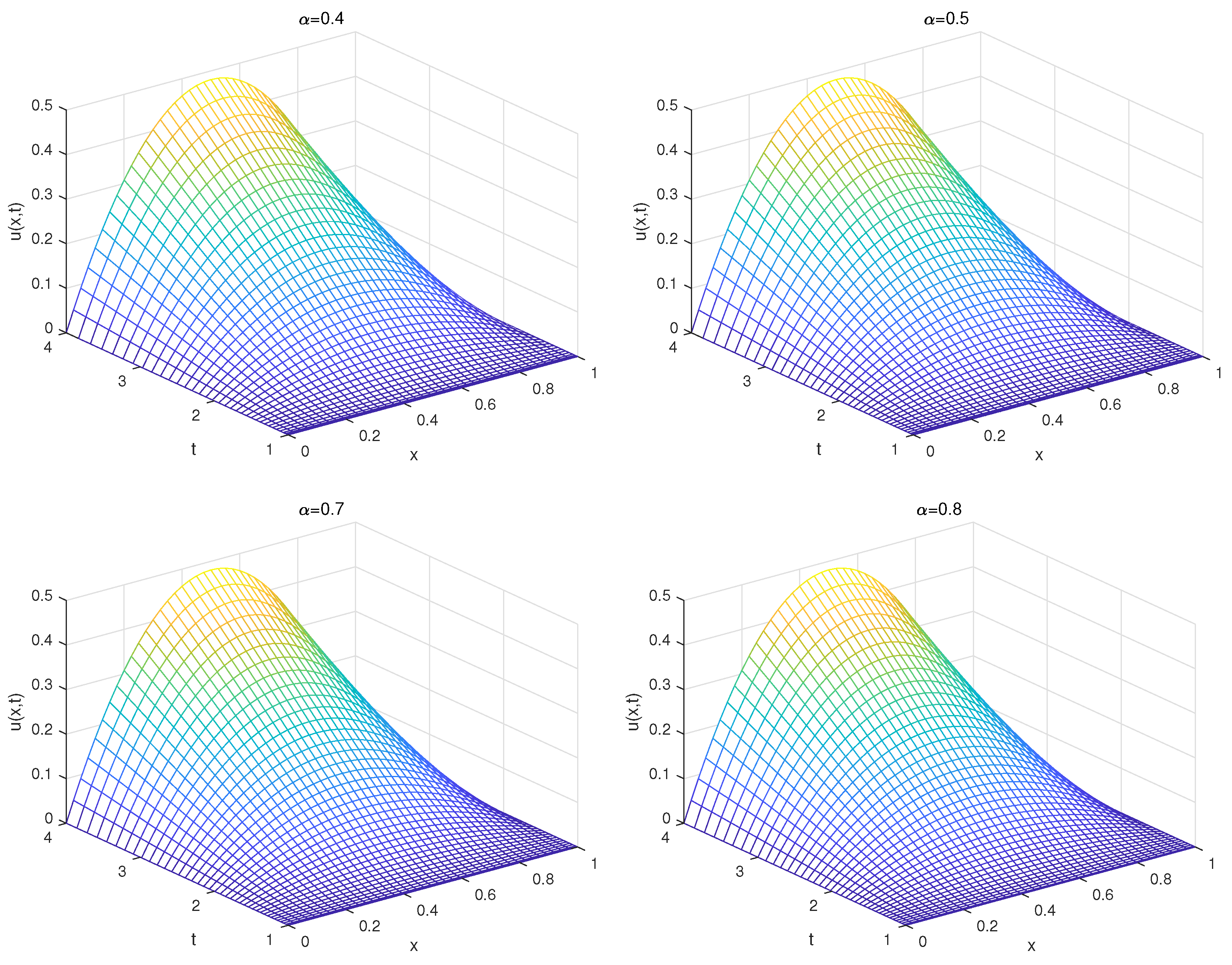
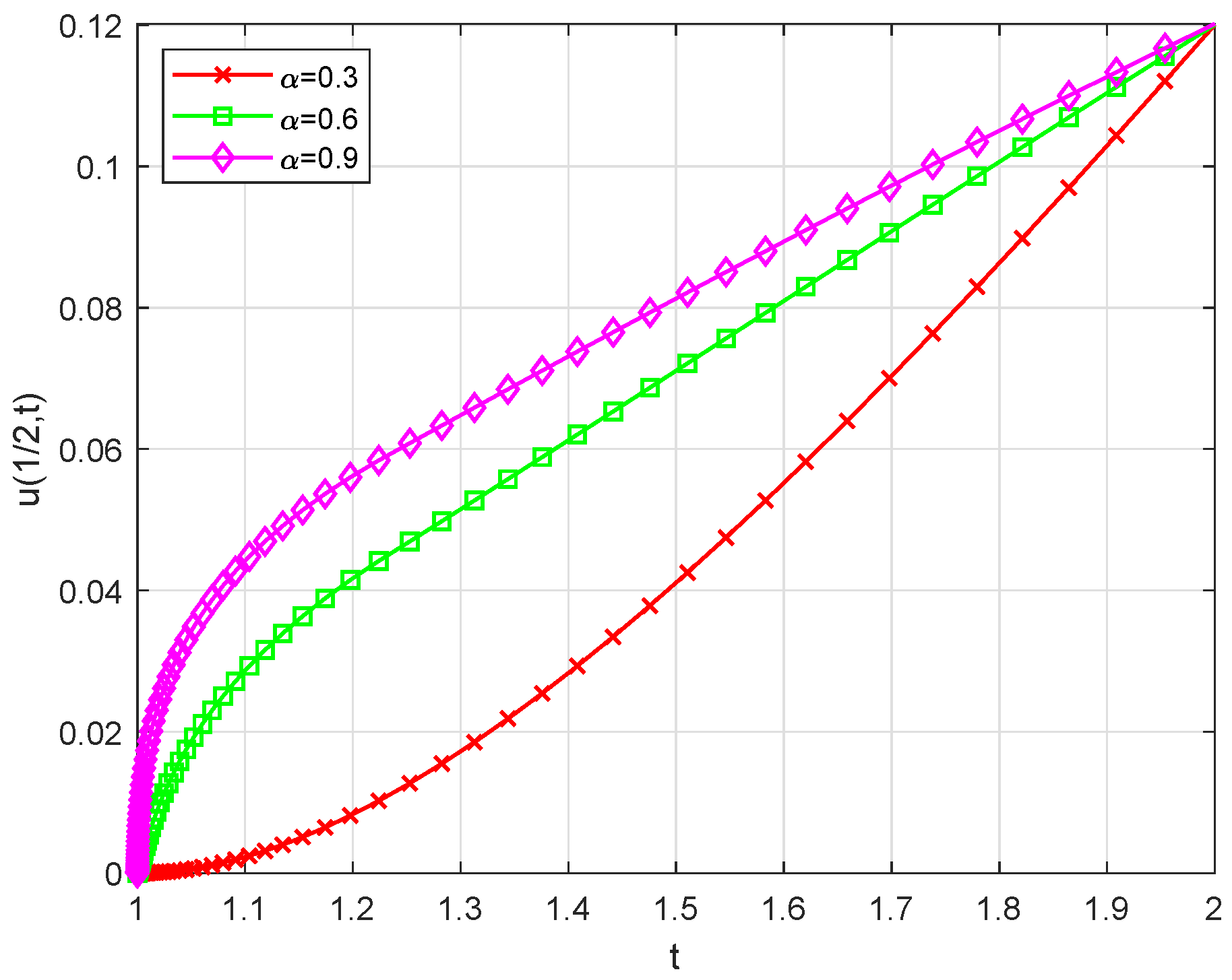
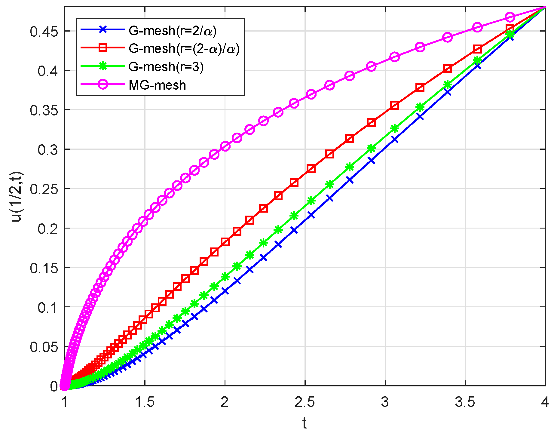
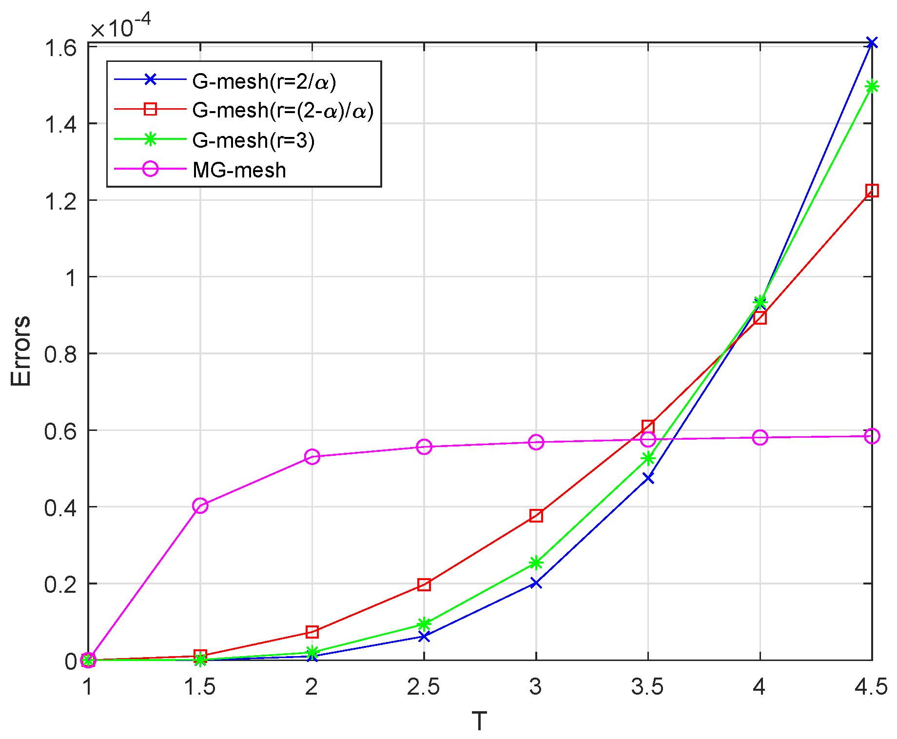
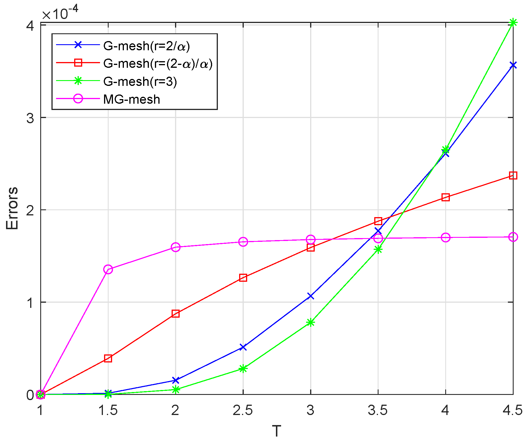
5. Numerical Experiments and Discussion

In this section, we present an example to verify the effectiveness and accuracy of our proposed numerical method. The maximum errors and rates of convergence are given by

$$E_2(M,N)=\underset{0\le n\le N}{max}∥e^n∥,Rate={\log }_2\left({\displaystyle \frac{E_2(M,N/2)}{E_2(M,N)}}\right),$$

respectively. In all calculations below, we choose the mesh parameter $K=\log \left(1.2\right)$.

Example 1.

The following problem is considered:

$$\left\{\begin{array}{cc}{}_{\mathit{CH}}\mathrm{D}_{1,t}^{\alpha }u(x,t)-{\displaystyle \frac{{\partial }^{2}u(x,t)}{\partial x^2}}=f(x,t),\hfill & 1<t\le T,0<x<1,\hfill \\ u(x,1)=0,\hfill & 0<x<1,\hfill \\ u(0,t)=u(1,t)=0,\hfill & 1<t\le T,\hfill \end{array}\right.$$

(47)

where $\alpha \in (0,1)$ and the source term:

$$f(x,t)={\displaystyle \frac{2}{\Gamma (3-\alpha )}}{\left(\log t\right)}^{2-\alpha }x(1-x)+2{\left(\log t\right)}^2.$$

The exact solution of this equation is $u(x,t)=x(1-x){\left(\log t\right)}^2.$

Let $h={\displaystyle \frac{1}{1024}}$ and $T=4$, the maximum errors and the corresponding orders of convergence with different values of $\alpha$ are given in

Table 1. Numerical results by using different meshes with $\alpha =0.4$ and $T=4$.

Grid	Parameter	$\mathit{N}=40$	$\mathit{N}=80$	$\mathit{N}=160$	$\mathit{N}=320$	$\mathit{N}=640$	$\mathit{N}=1280$
MG-mesh	$K=\log \left(1.2\right)$	$5.6810\times {10}^{-5}$	$1.9106\times {10}^{-5}$	$6.3938\times {10}^{-6}$	$2.1320\times {10}^{-6}$	$7.0897\times {10}^{-7}$	$2.3528\times {10}^{-7}$
			1.5721	1.5793	1.5845	1.5884	1.5913
G-mesh	$r={\displaystyle \frac{2}{\alpha }}$	$4.1441\times {10}^{-4}$	$1.4855\times {10}^{-4}$	$5.1878\times {10}^{-5}$	$1.7816\times {10}^{-5}$	$6.0501\times {10}^{-5}$	$2.0385\times {10}^{-6}$
			1.4801	1.5178	1.5419	1.5581	1.5695
	$r={\displaystyle \frac{2-\alpha }{\alpha }}$	$3.0148\times {10}^{-4}$	$1.0680\times {10}^{-4}$	$3.7018\times {10}^{-5}$	$1.2650\times {10}^{-5}$	$4.2809\times {10}^{-6}$	$1.4390\times {10}^{-6}$
			1.4972	1.5286	1.5491	1.5632	1.5728
	$r=3$	$1.9919\times {10}^{-4}$	$6.9641\times {10}^{-5}$	$2.3933\times {10}^{-5}$	$8.1314\times {10}^{-6}$	$2.7408\times {10}^{-6}$	$9.1863\times {10}^{-7}$
			1.5161	1.5409	1.5574	1.5689	1.5770

,

Table 2. Numerical results by using different meshes with $\alpha =0.5$ and $T=4$.

Grid	Parameter	$\mathit{N}=40$	$\mathit{N}=80$	$\mathit{N}=160$	$\mathit{N}=320$	$\mathit{N}=640$	$\mathit{N}=1280$
MG-mesh	$K=\log \left(1.2\right)$	$8.8474\times {10}^{-5}$	$3.1626\times {10}^{-5}$	$1.1268\times {10}^{-5}$	$4.0052\times {10}^{-6}$	$1.4214\times {10}^{-6}$	$5.0388\times {10}^{-7}$
			1.4841	1.4889	1.4923	1.4946	1.4962
G-mesh	$r={\displaystyle \frac{2}{\alpha }}$	$4.7929\times {10}^{-4}$	$1.7941\times {10}^{-4}$	$6.5848\times {10}^{-5}$	$2.3871\times {10}^{-5}$	$8.5847\times {10}^{-6}$	$3.0709\times {10}^{-6}$
			1.4176	1.4460	1.4639	1.4754	1.4831
	$r={\displaystyle \frac{2-\alpha }{\alpha }}$	$3.2361\times {10}^{-4}$	$1.1969\times {10}^{-4}$	$4.3599\times {10}^{-5}$	$1.5729\times {10}^{-5}$	$5.6385\times {10}^{-5}$	$2.0127\times {10}^{-5}$
			1.4350	1.4569	1.4709	1.4800	1.4862
	$r=3$	$3.2361\times {10}^{-4}$	$1.1969\times {10}^{-4}$	$4.3599\times {10}^{-5}$	$1.5729\times {10}^{-5}$	$5.6385\times {10}^{-6}$	$2.0127\times {10}^{-6}$
			1.4350	1.4569	1.4709	1.4800	1.4862

,

Table 3. Numerical results by using different meshes with $\alpha =0.6$ and $T=4$.

Grid	Parameter	$\mathit{N}=40$	$\mathit{N}=80$	$\mathit{N}=160$	$\mathit{N}=320$	$\mathit{N}=640$	$\mathit{N}=1280$
MG-mesh	$K=\log \left(1.2\right)$	$1.4010\times {10}^{-4}$	$5.3405\times {10}^{-5}$	$2.0315\times {10}^{-5}$	$7.7175\times {10}^{-6}$	$2.9293\times {10}^{-6}$	$1.1112\times {10}^{-6}$
			1.3914	1.3944	1.3963	1.3976	1.3984
G-mesh	$r={\displaystyle \frac{2}{\alpha }}$	$5.8056\times {10}^{-4}$	$2.{2865}^{-4}s$	$8.8743\times {10}^{-5}$	$3.4140\times {10}^{-5}$	$1.3062\times {10}^{-5}$	$4.9806\times {10}^{-6}$
			1.3443	1.3654	1.3782	1.3861	1.3910
	$r={\displaystyle \frac{2-\alpha }{\alpha }}$	$3.6620\times {10}^{-4}$	$1.4255\times {10}^{-4}$	$5.4939\times {10}^{-5}$	$2.1044\times {10}^{-5}$	$8.0296\times {10}^{-6}$	$3.0563\times {10}^{-6}$
			1.3612	1.3756	1.3844	1.3900	1.3935
	$r=3$	5.0684e-04	$1.9887\times {10}^{-4}$	$7.7015\times {10}^{-5}$	$2.9587\times {10}^{-5}$	$1.1311\times {10}^{-5}$	$4.3104\times {10}^{-6}$
			1.3497	1.3686	1.3802	1.3872	1.3918

,

Table 4. Numerical results by using different meshes with $\alpha =0.7$ and $T=4$.

Grid	Parameter	$\mathit{N}=40$	$\mathit{N}=80$	$\mathit{N}=160$	$\mathit{N}=320$	$\mathit{N}=640$	$\mathit{N}=1280$
MG-mesh	$K=\log \left(1.2\right)$	$2.2373\times {10}^{-4}$	$9.1136\times {10}^{-5}$	$3.7080\times {10}^{-5}$	$1.5076\times {10}^{-5}$	$6.1268\times {10}^{-6}$	$2.4893\times {10}^{-6}$
			1.2957	1.2974	1.2984	1.2990	1.2994
G-mesh	$r={\displaystyle \frac{2}{\alpha }}$	$7.2998\times {10}^{-4}$	$3.0416\times {10}^{-4}$	$1.2540\times {10}^{-4}$	$5.1382\times {10}^{-5}$	$2.0979\times {10}^{-5}$	$8.5475\times {10}^{-6}$
			1.2630	1.2783	1.2872	1.2923	1.2954
	$r={\displaystyle \frac{2-\alpha }{\alpha }}$	$4.3372\times {10}^{-4}$	$1.7877\times {10}^{-4}$	$7.3245\times {10}^{-5}$	$2.9903\times {10}^{-5}$	$1.2183\times {10}^{-5}$	$4.9572\times {10}^{-6}$
			1.2787	1.2873	1.2924	1.2954	1.2973
	$r=3$	$7.7424\times {10}^{-4}$	$3.2307\times {10}^{-4}$	$1.3330\times {10}^{-4}$	$5.4647\times {10}^{-5}$	$2.2318\times {10}^{-5}$	$9.0947\times {10}^{-6}$
			1.2609	1.2772	1.2865	1.2919	1.2951

and

Table 5. Numerical results by using different meshes with $\alpha =0.8$ and $T=4$.

Grid	Parameter	$\mathit{N}=40$	$\mathit{N}=80$	$\mathit{N}=160$	$\mathit{N}=320$	$\mathit{N}=640$	$\mathit{N}=1280$
MG-mesh	$K=\log \left(1.2\right)$	$3.5835\times {10}^{-4}$	$1.5619\times {10}^{-4}$	$6.8038\times {10}^{-5}$	$2.9628\times {10}^{-5}$	$1.2899\times {10}^{-5}$	$5.6156\times {10}^{-6}$
			1.1981	1.1989	1.1994	1.1997	1.1997
G-mesh	$r={\displaystyle \frac{2}{\alpha }}$	$9.4673\times {10}^{-4}$	$4.1903\times {10}^{-4}$	$1.8409\times {10}^{-4}$	$8.0541\times {10}^{-5}$	$3.5158\times {10}^{-5}$	$1.5328\times {10}^{-5}$
			1.1759	1.1866	1.1926	1.1959	1.1977
	$r={\displaystyle \frac{2-\alpha }{\alpha }}$	$5.3493\times {10}^{-4}$	$2.3451\times {10}^{-4}$	$1.0248\times {10}^{-4}$	$4.4707\times {10}^{-5}$	$1.9484\times {10}^{-5}$	$8.4869\times {10}^{-6}$
			1.1897	1.1943	1.1968	1.1982	1.1990
	$r=3$	$1.1611\times {10}^{-3}$	$5.1619\times {10}^{-4}$	$2.2731\times {10}^{-4}$	$9.9585\times {10}^{-5}$	$4.3504\times {10}^{-5}$	$1.8975\times {10}^{-5}$
			1.1695	1.1832	1.1907	1.1948	1.1970

. For the sake of comparison, we also apply the $L1$ scheme on a graded mesh to approximate the time fractional derivative, utilizing parameters $r=2/\alpha ,r=(2-\alpha )/\alpha$, and $r=3$. The outcomes of these computations are presented in Table 1, Table 2, Table 3, Table 4 and Table 5. It is evident that these numerical findings align with the theoretical predictions outlined in Theorem 2. Meanwhile, it is shown from these numerical results that both our proposed MG-mesh, which incorporates the parameter $K\in (0,\log T)$ and the graded mesh defined by Equation (2) with $r\ge {\displaystyle \frac{2-\alpha }{\alpha }}$ attain the optimal convergence rate of $O\left(N^{-(2-\alpha )}\right)$. This indicates that both meshing strategies are efficient and effective in terms of achieving the desired convergence rate. However, it is worth noting that despite both methods achieving the optimal convergence rate of $O\left(N^{-(2-\alpha )}\right)$, the maximum errors obtained using our proposed MG-mesh are the lowest. This result can be seen in Table 1, Table 2, Table 3, Table 4 and Table 5. For example, by fixing $M=1024,\alpha =0.4$ in Table 1 and varying N, both cases achieve the optimal convergence rate for different rank indices r. For fixed N, the MG-mesh exhibits substantially reduced errors relative to the G-mesh. A representative case at $N=1280$ shows that the G-mesh error exceeds the MG-mesh error by nearly one order of magnitude, while its convergence order remains inferior. The results in Table 2, Table 3, Table 4 and Table 5 align with the observations from Table 1. This suggests that our MG-mesh may offer additional benefits in terms of accuracy compared to the G-mesh defined by Equation (2).

For $M=N=80$ and different values of $\alpha$, Figure 3 visually presents the numerical solutions corresponding to various fractional orders $\alpha$. A detailed cross-sectional analysis at $x={\displaystyle \frac{1}{2}}$ under different $\alpha$ values is subsequently illustrated in Figure 4, while Figure 5 provides a comparative visualization of numerical solutions obtained from the MG-mesh versus standard graded meshes (G-meshes) with parameters $N=80$, $\alpha =0.6$, and varying mesh refinement ratios r. Additionally, we compare the errors and convergence rates obtained on our proposed MG-mesh (8) with those on the optimal graded meshes (1). Our observations indicate that in these scenarios, the optimal global rates of convergence of $2-\alpha$ are achieved. Moreover, as time T increases, the errors decrease. Notably, the errors calculated on the MG-mesh are significantly smaller than those on graded meshes for each given time length T. Figure 6 and Figure 7, respectively, demonstrate the variation of errors as time progresses.

6. Conclusions

In this paper, a modified graded mesh (MG-mesh) is used as the discretization mesh of the $L1$ interpolation method to approximate the Caputo–Hadamard fractional sub-diffusion equation derivative of time fractional diffusion Equation (2). Comparing the numerical results for both schemes, we can observe that the MG-mesh scheme performs better than the graded mesh (1) (G-mesh) scheme for the sub-diffusion equations. The $L1$ on this MG-mesh with optimal $2-\alpha$-order accuracy has been proved. Its error is also significantly smaller than that of the G-mesh grid. This study also shows that the MG-mesh we proposed with $K\in (0,\log T)$ can obtain the optimal convergence rate $O\left(N^{-(2-\alpha )}\right)$. Furthermore, we observe that the final result obviously shows how the regularity of the solution and the nonuniform meshes affect the convergence order of the derived scheme. The convergence order of the numerical results matches that of the theoretical ones.

Our future work for this proposed method includes accelerating the approximation of the Caputo–Hadamard time-fractional derivative in Equation (2) by using the sum-of-exponentials strategy [19] and parallel computations [27,28].

References

1. Vellappandi, M.; Govindaraj, V. Operator theoretic approach to optimal control problems characterized by the Caputo fractional differential equations. Res. Control Optim. 2023, 10, 100194. [Google Scholar] [CrossRef]
2. Giona, M.; Roman, H.E. Fractional diffusion equation for transport phenomena in random media. Physica A 1992, 185, 87–97. [Google Scholar] [CrossRef]
3. Gorenflo, R.; Mainardi, F.; Moretti, D.; Pagnini, G.; Paradisi, P. Discrete random walk models for space–time fractional diffusion. Chem. Phys. 2002, 284, 521–541. [Google Scholar] [CrossRef]
4. Huong, N.T.T.; Thang, N.N.; Ke, T.D. Commutator of the Caputo fractional derivative and the shift operator and applications. Commun. Nonlinear Sci. Numer. Simul. 2024, 131, 107857. [Google Scholar] [CrossRef]
5. Fahad, H.M.; Fernandez, A. Operational calculus for Caputo fractional calculus with respect to functions and the associated fractional differential equations. Appl. Math. Comput. 2021, 409, 126400. [Google Scholar] [CrossRef]
6. Green, C.; Liu, Y.; Yan, Y. Numerical methods for Caputo-Hadamard fractional differential equations with graded and non-uniform meshes. Mathematics 2021, 9, 2728. [Google Scholar] [CrossRef]
7. Sivalingam, S.; Kumar, P.; Govindaraj, V. A neural networks-based numerical method for the generalized Caputo-type fractional differential equations. Math. Comput. Simul. 2023, 213, 302–323. [Google Scholar]
8. Fan, E.; Li, C.; Li, Z. Numerical approaches to Caputo-Hadamard fractional derivatives with applications to long-term integration of fractional differential systems. Commun. Nonlinear Sci. Numer. Simul. 2022, 106, 106096. [Google Scholar] [CrossRef]
9. Liu, C.-X.; Cao, J.-Y.; Lyu, T.; Ye, X.-Y. Numerical Analysis of a High-Order Scheme with Nonuniform Time Grids for Caputo-Hadamard Fractional Reaction Sub-diffusion Equations. Commun. Appl. Math. Comput. 2024, 1–28. [Google Scholar] [CrossRef]
10. Hadamard, J. Essai sur l’étude des fonctions données par leur développement de taylor. J. Math. Pures Appl. 1892, 8, 101–186. [Google Scholar]
11. Kilbas, A.A. Hadamard-type fractional calculus. J. Korean Math. Soc. 2001, 38, 1191–1204. [Google Scholar]
12. Jarad, F.; Abdeljawad, T.; Baleanu, D. Caputo-type modification of the Hadamard fractional derivatives. Adv. Differ. Equ. 2012, 2012, 142. [Google Scholar] [CrossRef]
13. Ma, L.; Li, C. On Hadamard fractional calculus. Fractals 2017, 25, 1750033. [Google Scholar] [CrossRef]
14. Ma, L.; Li, C. On finite part integrals and Hadamard-type fractional derivatives. J. Comput. Nonlinear Dyn. 2018, 13, 090905. [Google Scholar] [CrossRef]
15. Li, C.; Li, Z. Stability and logarithmic decay of the solution to Hadamard-type fractional differential equation. J. Nonlinear Sci. 2021, 31, 31. [Google Scholar] [CrossRef]
16. Zheng, X. Logarithmic transformation between (variable-order) caputo and Caputo-Hadamard fractional problems and applications. Appl. Math. Lett. 2021, 121, 107366. [Google Scholar] [CrossRef]
17. Zaky, M.A.; Hendy, A.S.; Suragan, D. Logarithmic jacobi collocation method for Caputo-Hadamard fractional differential equations. Appl. Numer. Math. 2022, 181, 326–346. [Google Scholar] [CrossRef]
18. Zhao, T.; Li, C.; Li, D. Efficient spectral collocation method for fractional differential equation with Caputo-Hadamard derivative. Fract. Calc. Appl. Anal. 2023, 26, 2903–2927. [Google Scholar] [CrossRef]
19. He, T.; Lu, J.; Li, M. The parareal algorithm for Caputo-Hadamard fractional differential equations. Commun. Anal. Comput. 2024, 2, 432–453. [Google Scholar] [CrossRef]
20. Gohar, M.; Li, C.; Li, Z. Finite difference methods for Caputo–Hadamard fractional differential equations. Mediterr. J. Math. 2020, 17, 194. [Google Scholar] [CrossRef]
21. Li, C.; Li, Z.; Wang, Z. Mathematical analysis and the local discontinuous galerkin method for Caputo-Hadamard fractional partial differential equation. J. Sci. Comput. 2020, 85, 41. [Google Scholar] [CrossRef]
22. Wang, Z.; Ou, C.; Vong, S. A second-order scheme with nonuniform time grids for Caputo–Hadamard fractional sub-diffusion equations. J. Comput. Appl. Math. 2022, 414, 114448. [Google Scholar] [CrossRef]
23. Wang, Z.; Sun, L. A numerical approximation for the Caputo-Hadamard derivative and its application in time-fractional variable-coefficient diffusion equation. Discret. Contin. Dyn.-Syst.-S. 2024, 17, 2679–2705. [Google Scholar] [CrossRef]
24. Ou, C.; Cen, D.; Wang, Z.; Vong, S. Fitted schemes for Caputo-Hadamard fractional differential equations. Numer. Algorithms 2024, 97, 135–164. [Google Scholar] [CrossRef]
25. Liu, L.-B.; Xu, L.; Zhang, Y. Error analysis of a finite difference scheme on a modified graded mesh for a time-fractional diffusion equation. Math. Comput. Simul. 2023, 209, 87–101. [Google Scholar] [CrossRef]
26. Stynes, M.; O’Riordan, E.; Gracia, J.L. Error analysis of a finite difference method on graded meshes for a time-fractional diffusion equation. SIAM J. Numer. Anal. 2017, 55, 1057–1079. [Google Scholar] [CrossRef]
27. Gu, X.-M.; Wu, S.-L. A parallel-in-time iterative algorithm for Volterra partial integro-differential problems with weakly singular kernel. J. Comput. Phys. 2020, 417, 109576. [Google Scholar] [CrossRef]
28. Zhao, Y.-L.; Gu, X.-M.; Ostermann, A. A preconditioning technique for an all-at-once system from Volterra subdiffusion equations with graded time steps. J. Sci. Comput. 2021, 88, 11. [Google Scholar] [CrossRef]
Figure 1. Comparison of the MG-mesh and G-mesh mesh fetch points at time N = 40 , T = 4 and α = 0.3 .
Fractalfract 09 00286 g001
Figure 2. Comparison of the MG-mesh and G-mesh mesh fetch points at time N = 40 , T = 4 and α = 0.8 .
Fractalfract 09 00286 g002
Figure 3. Numerical solutions with M = N = 40 and different α .
Fractalfract 09 00286 g003
Figure 4. Numerical solutions with M = N = 80 and different α at x = 1 / 2 .
Fractalfract 09 00286 g004
Figure 5. Numerical solutions between MG-mesh and G-mesh with α = 0.6 and different r at x = 1 / 2 .
Fractalfract 09 00286 g005
Figure 6. Comparison of errors between the MG-mesh and G-mesh with N = 80 and α = 0.6 .
Fractalfract 09 00286 g006
Figure 7. Comparison of errors between the MG-mesh and G-mesh with N = 80 and α = 0.8 .
Fractalfract 09 00286 g007