
Duality Revelation and Operator-Based Method in Viscoelastic Problems


Abstract
1. Introduction
2. Classical Linear Viscoelastic Theory
2.1. Creep Function and Relaxation Function
2.2. General Differential Constitutive Models
3. Operator-Based Method to Viscoelastic Quasi-Static Mechanical Analysis
3.1. Operator-Based Method Based on LT
3.2. Consistency with Operational Calculus
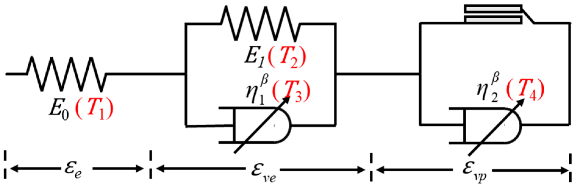
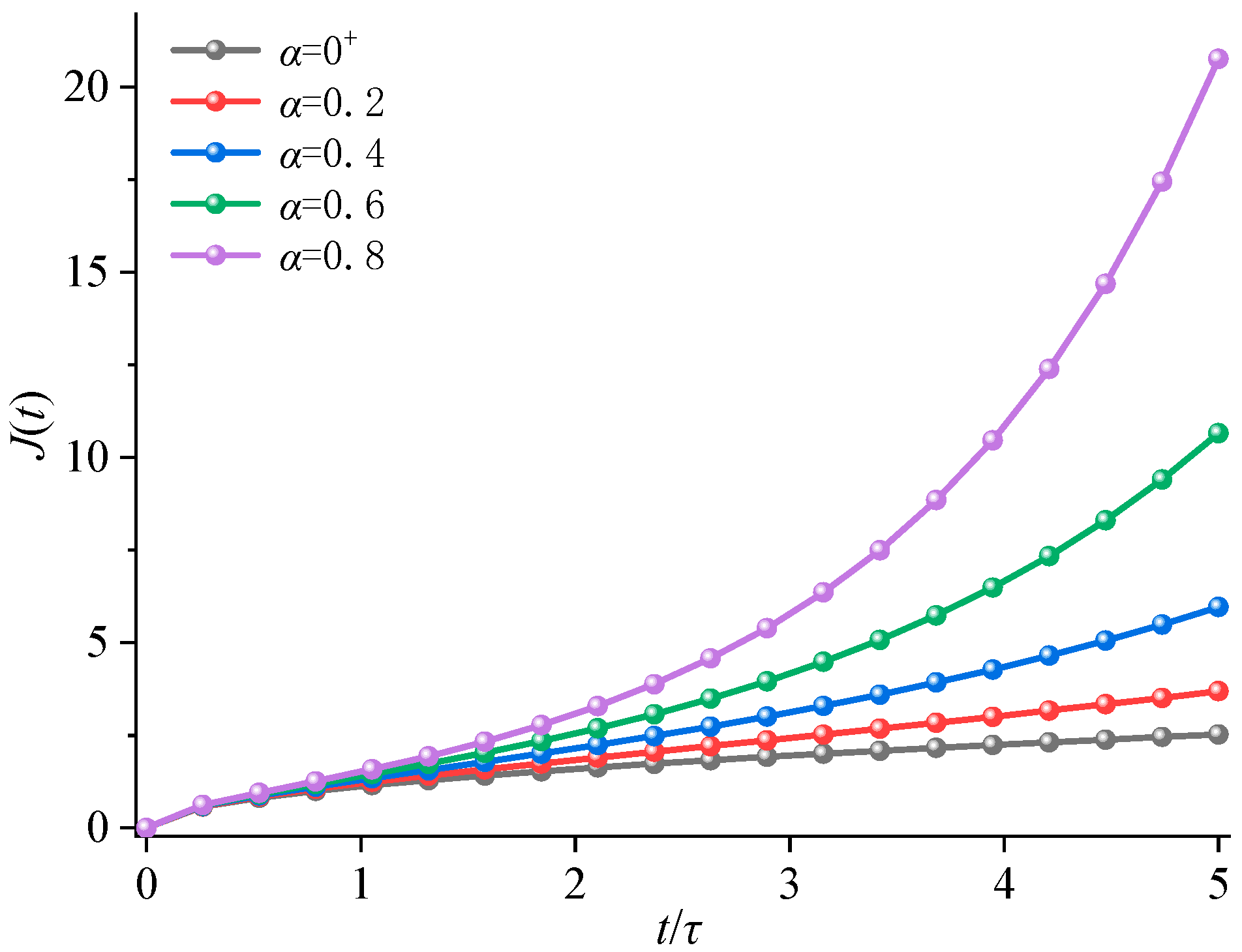
3.3. Operator-Based Method for Fractional Differential Constitutive Models
4. Operator-Based Method to Viscoelastic Dynamic Mechanical Analysis
4.1. Operator-Based Method to Complex Modulus and Complex Compliance
- Compute the total stiffness operator of the structure;
- Substitute the differential operator with the complex variable in , yielding the dynamic complex modulus. The resultant real and imaginary components correspond to the storage modulus and loss modulus, respectively;
- Calculate the loss factor as the ratio of imaginary-to-real components.
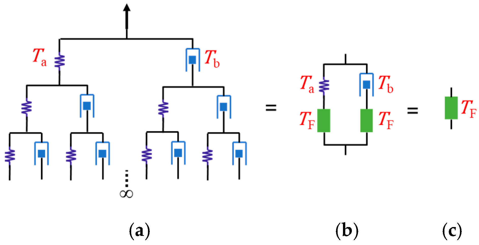
4.2. Dynamic Performance Analysis of Fractal Tree Structure
5. Discussion
5.1. Operator-Based Method for Creep Functions with Variable Coefficients
5.2. Creep Function of Physical Fractal Structure with Variable Coefficient
6. Conclusions
- The operator-based method enhances the mathematical duality between the creep and relaxation functions, offering greater physical intuition and an intuitive understanding of time-dependent material behavior. It directly reflects the intrinsic properties of the system, independent of input and output conditions.
- The method is extended to dynamic problems, where the complex modulus and complex compliance are derived through operator representations. The fractal tree model, with its constant loss factor across the entire frequency spectrum, demonstrates its potential engineering value.
- By introducing a damage-based variable coefficient to the fractal tree model, it now has the potential to describe the accelerated creep phase of rocks. This enhancement allows the model to account for damage evolution in rock materials under prolonged loading, particularly during the accelerated creep stage. However, further experimental validation is required to fully substantiate its practical application.
Author Contributions
Funding
Data Availability Statement
Acknowledgments
Conflicts of Interest
Appendix A

- Two equilibrium equations expressed in terms of stress:
- Two compatibility equations expressed in terms of strain:
- Three constitutive relations for individual components:

| Model | Maxwell | Kelvin-Voigt | Zener | Generalized Kelvin-Voigt | Fractal Tree |
|---|---|---|---|---|---|
| Schematic |  |  | 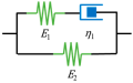 | 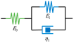 |  |
Appendix B
References
- Wu, J.; Yang, Y.; Mehrabi, P.; Nasr, E.A. Efficient Machine-Learning Algorithm Applied to Predict the Transient Shock Reaction of the Elastic Structure Partially Rested on the Viscoelastic Substrate. Mech. Adv. Mater. Struct. 2024, 31, 3700–3724. [Google Scholar] [CrossRef]
- Deng, J.; Ortega, J.E.B.; Liu, K.; Gong, Y. Theoretical and Numerical Investigations on Dynamic Stability of Viscoelastic Columns with Semi-Rigid Connections. Thin-Walled Struct. 2024, 198, 111758. [Google Scholar] [CrossRef]
- Tringides, C.M.; Vachicouras, N.; De Lázaro, I.; Wang, H.; Trouillet, A.; Seo, B.R.; Elosegui-Artola, A.; Fallegger, F.; Shin, Y.; Casiraghi, C.; et al. Viscoelastic Surface Electrode Arrays to Interface with Viscoelastic Tissues. Nat. Nanotechnol. 2021, 16, 1019–1029. [Google Scholar] [CrossRef] [PubMed]
- Sevenler, D.; Toner, M. High Throughput Intracellular Delivery by Viscoelastic Mechanoporation. Nat. Commun. 2024, 15, 115. [Google Scholar] [CrossRef]
- Ye, H.; Wu, B.; Sun, S.; Wu, P. Self-Compliant Ionic Skin by Leveraging Hierarchical Hydrogen Bond Association. Nat. Commun. 2024, 15, 885. [Google Scholar] [CrossRef]
- Zhou, X.; Fu, W.; Wang, Y.; Yan, H.; Huang, Y. Impact Responses and Wave Dissipation Investigation of a Composite Sandwich Shell Reinforced by Multilayer Negative Poisson’s Ratio Viscoelastic Polymer Material Honeycomb. Materials 2023, 17, 233. [Google Scholar] [CrossRef]
- Xue, Y.; Liu, J.; Ranjith, P.G.; Zhang, Z.; Gao, F.; Wang, S. Experimental Investigation on the Nonlinear Characteristics of Energy Evolution and Failure Characteristics of Coal under Different Gas Pressures. Bull. Eng. Geol. 2022, 81, 1–26. [Google Scholar] [CrossRef]
- Chen, B.; Lai, Z.; Lai, X.; Varma, A.H.; Yu, X. Creep-Prediction Models for Concrete-Filled Steel Tube Arch Bridges. J. Bridge Eng. 2017, 22, 04017027. [Google Scholar] [CrossRef]
- Bischoff, D.J.; Lee, T.; Kang, K.-S.; Molineux, J.; O’Neil Parker, W.; Pyun, J.; Mackay, M.E. Unraveling the Rheology of Inverse Vulcanized Polymers. Nat. Commun. 2023, 14, 7553. [Google Scholar] [CrossRef]
- Christensen, R.M. Theory of Viscoelasticity: An Introduction, 2nd ed.; Academic Press: New York, NY, USA, 1982; ISBN 978-0-12-174252-2. [Google Scholar]
- Blair, G.S. The Role of Psychophysics in Rheology. J. Colloid. Sci. 1947, 2, 21–32. [Google Scholar] [CrossRef]
- Wu, F.; Chen, J.; Zou, Q. A Nonlinear Creep Damage Model for Salt Rock. Int. J. Damage Mech. 2019, 28, 758–771. [Google Scholar] [CrossRef]
- Chen, W. Time–Space Fabric Underlying Anomalous Diffusion. Chaos Solitons Fract. 2006, 28, 923–929. [Google Scholar] [CrossRef]
- Chen, Y.; Hao, X.; Xue, D.; Li, Z.; Ma, X. Creep Behavior and Permeability Evolution of Coal Pillar Dam for Underground Water Reservoir. Int. J. Coal Sci. Technol. 2023, 10, 11. [Google Scholar] [CrossRef]
- Liu, Z.; Yu, X.; Xie, S.; Zhou, H.; Yin, Y. Fractional Derivative Model on Physical Fractal Space: Improving Rock Permeability Analysis. Fractal Fract. 2024, 8, 470. [Google Scholar] [CrossRef]
- Sales Teodoro, G.; Tenreiro Machado, J.A.; Capelas De Oliveira, E. A Review of Definitions of Fractional Derivatives and Other Operators. J. Comput. Phys. 2019, 388, 195–208. [Google Scholar] [CrossRef]
- Zhang, Y.; Sun, H.; Stowell, H.H.; Zayernouri, M.; Hansen, S.E. A Review of Applications of Fractional Calculus in Earth System Dynamics. Chaos Solitons Fract. 2017, 102, 29–46. [Google Scholar] [CrossRef]
- Hu, K.X.; Zhu, K.Q. Mechanical Analogies of Fractional Elements. Chin. Phys. Lett. 2009, 26, 108301. [Google Scholar] [CrossRef]
- Yang, F.; Zhu, K.Q. On the Definition of Fractional Derivatives in Rheology. Theor. Appl. Mech. Lett. 2011, 1, 012007. [Google Scholar] [CrossRef]
- Guo, J.Q.; Yin, Y.J.; Ren, G.X. Abstraction and Operator Characterization of Fractal Ladder Viscoelastic Hyper-Cell for Ligaments and Tendons. Appl. Math. Mech. 2019, 40, 1429–1448. [Google Scholar] [CrossRef]
- Jian, Z.M.; Guo, J.Q.; Peng, G.; Yin, Y.J. Fractal Operators and Fractional-Order Mechanics of Bone. Fract. Fract. 2023, 7, 642. [Google Scholar] [CrossRef]
- Paola, M.D.; Zingales, M. Exact Mechanical Models of Fractional Hereditary Materials. J. Rheol. 2012, 56, 983–1004. [Google Scholar] [CrossRef]
- Yin, Y.J.; Peng, G.; Yu, X.B. Algebraic Equations and Non-Integer Orders of Fractal Operators Abstracted from Biomechanics. Acta Mech. Sin. 2022, 38, 521488. [Google Scholar] [CrossRef]
- Liu, Z.L.; Yu, X.B.; Zhang, S.; Zhou, H.; Yin, Y.J. Modeling the Creep Behavior of Coal in a Physical Fractal Framework. Mech. Time-Depend. Mater. 2025, 29, 13. [Google Scholar] [CrossRef]
- Yu, X.B.; Yin, Y.J. Fractal Operators and Convergence Analysis in Fractional Viscoelastic Theory. Fract. Fract. 2024, 8, 200. [Google Scholar] [CrossRef]
- Heaviside, O. On Operators in Physical Mathematics. Part I. Proc. R. Soc. Lond. 1893, 52, 504–529. [Google Scholar] [CrossRef]
- Mikusiński, J. Operational Calculus, 2nd ed.; Pergamon Press: Oxford, UK, 1983. [Google Scholar]
- Yu, X.B.; Yin, Y.J. Operator Kernel Functions in Operational Calculus and Applications in Fractals with Fractional Operators. Fract. Fract. 2023, 7, 755. [Google Scholar] [CrossRef]
- Wu, F.; Liu, J.F.; Wang, J. An Improved Maxwell Creep Model for Rock Based on Variable-Order Fractional Derivatives. Environ. Earth Sci. 2015, 73, 6965–6971. [Google Scholar] [CrossRef]
- Zhou, F.; Wang, L.; Liu, H. A Fractional Elasto-Viscoplastic Model for Describing Creep Behavior of Soft Soil. Acta Geotech. 2021, 16, 67–76. [Google Scholar] [CrossRef]
- Liu, X.; Li, D.; Han, C.; Shao, Y. A Caputo Variable-Order Fractional Damage Creep Model for Sandstone Considering Effect of Relaxation Time. Acta Geotech. 2022, 17, 153–167. [Google Scholar] [CrossRef]
- Ren, S.; Wang, H.; Ni, W.; Wu, B. A New One-Dimensional Consolidation Creep Model for Clays. Comput. Geotech. 2024, 169, 106214. [Google Scholar] [CrossRef]
- Liu, Z.L.; Yu, X.B.; Yin, Y.J. On the Rigorous Correspondence Between Operator Fractional Powers and Fractional Derivatives via the Sonine Kernel. Fractal Fract. 2024, 8, 653. [Google Scholar] [CrossRef]
- Podlubny, I. Fractional Differential Equations; Academic Press: San Diego, CA, USA, 1999. [Google Scholar]
- Caputo, M. Linear Models of Dissipation Whose Q Is Almost Frequency Independent. Ann. Geophys. 1966, 19, 383–393. [Google Scholar] [CrossRef]
- Caputo, M. Linear Models of Dissipation Whose Q Is Almost Frequency Independent-II. Geophys. J. R. Astron. Soc. 1967, 13, 529–539. [Google Scholar] [CrossRef]
- Zhou, H.W.; Wang, C.P.; Han, B.B.; Duan, Z.Q. A Creep Constitutive Model for Salt Rock Based on Fractional Derivatives. Int. J. Rock. Mech. Min. Sci. 2011, 48, 116–121. [Google Scholar] [CrossRef]
- Xu, X.; Qiu, W.; Wan, D.; Wu, J.; Zhao, F.; Xiong, Y. Numerical Modelling of the Viscoelastic Polymer Melt Flow in Material Extrusion Additive Manufacturing. Virtual Phys. Prototyp. 2024, 19, e2300666. [Google Scholar] [CrossRef]
- Knight, J.; Salim, H.; Elemam, H.; Elbelbisi, A. Calibration of Thermal Viscoelastic Material Models for the Dynamic Responses of PVB and SG Interlayer Materials. Polymers 2024, 16, 1870. [Google Scholar] [CrossRef] [PubMed]
- Saba, N.; Jawaid, M.; Alothman, O.Y.; Paridah, M.T. A Review on Dynamic Mechanical Properties of Natural Fibre Reinforced Polymer Composites. Constr. Build. Mater. 2016, 106, 149–159. [Google Scholar] [CrossRef]
- Zhou, J.; Papautsky, I. Viscoelastic Microfluidics: Progress and Challenges. Microsyst. Nanoeng. 2020, 6, 113. [Google Scholar] [CrossRef]
- Lin, X.; Liu, Y.; Bai, A.; Cai, H.; Bai, Y.; Jiang, W.; Yang, H.; Wang, X.; Yang, L.; Sun, N.; et al. A Viscoelastic Adhesive Epicardial Patch for Treating Myocardial Infarction. Nat. Biomed. Eng. 2019, 3, 632–643. [Google Scholar] [CrossRef]
- Zhou, H.W.; Wang, C.P.; Mishnaevsky, L.; Duan, Z.Q.; Ding, J.Y. A Fractional Derivative Approach to Full Creep Regions in Salt Rock. Mech. Time-Depend. Mater. 2013, 17, 413–425. [Google Scholar] [CrossRef]


Disclaimer/Publisher’s Note: The statements, opinions and data contained in all publications are solely those of the individual author(s) and contributor(s) and not of MDPI and/or the editor(s). MDPI and/or the editor(s) disclaim responsibility for any injury to people or property resulting from any ideas, methods, instructions or products referred to in the content. |
© 2025 by the authors. Licensee MDPI, Basel, Switzerland. This article is an open access article distributed under the terms and conditions of the Creative Commons Attribution (CC BY) license (https://creativecommons.org/licenses/by/4.0/).
Share and Cite
Liu, Z.; Yu, X.; Yin, Y. Duality Revelation and Operator-Based Method in Viscoelastic Problems. Fractal Fract. 2025, 9, 274. https://doi.org/10.3390/fractalfract9050274
Liu Z, Yu X, Yin Y. Duality Revelation and Operator-Based Method in Viscoelastic Problems. Fractal and Fractional. 2025; 9(5):274. https://doi.org/10.3390/fractalfract9050274
Chicago/Turabian StyleLiu, Zelin, Xiaobin Yu, and Yajun Yin. 2025. "Duality Revelation and Operator-Based Method in Viscoelastic Problems" Fractal and Fractional 9, no. 5: 274. https://doi.org/10.3390/fractalfract9050274
APA StyleLiu, Z., Yu, X., & Yin, Y. (2025). Duality Revelation and Operator-Based Method in Viscoelastic Problems. Fractal and Fractional, 9(5), 274. https://doi.org/10.3390/fractalfract9050274