Free Metaplectic K-Wigner Distribution: Uncertainty Principles and Applications

Abstract

This study focuses on a novel parameterized Wigner distribution, which is an organic integration of the free metaplectic Wigner distribution and the $\mathbf{K}$-Wigner distribution. We style this as the free metaplectic $\mathbf{K}$-Wigner distribution (FMKWD) and investigate its uncertainty principles and related applications. We establish a crucial equivalence relation between the uncertainty product in time-FMKWD and free metaplectic transformation (FMT)-FMKWD domains and those in two FMT domains, from which we derive two types of orthogonality conditions: an orthonormality condition; and two sub-types of minimum or maximum eigenvalue commutativity conditions on the FMKWD. Finally we separately formulate an uncertainty inequality in FMKWD domains for real-valued functions, three kinds of uncertainty inequalities in orthogonal FMKWD domains, an uncertainty inequality in orthonormal FMKWD domains, and four kinds of uncertainty inequalities in the minimum or maximum eigenvalue commutative FMKWD domains for complex-valued functions. The time-frequency resolution of the FMKWD is compared with those of the free metaplectic Wigner distribution, $\mathbf{K}$-Wigner distribution, and N-dimensional Wigner distribution to demonstrate its superiority in super-resolution analysis. For applications, the uncertainty inequalities derived are used to estimate the bandwidth in FMKWD domains, and the FMKWD is applied to detect noisy linear frequency-modulated signals.

1. Introduction

The N-dimensional Wigner distribution [1,2] is one of the most fundamental non-stationary signals time-frequency analysis tools [3,4]. It has found many applications in mathematical physics [5,6], such as Fourier optics, matrix optics, radiometry, ray optics, wave optics, and geometrical optics.

Definition 1.

The N-dimensional Wigner distribution of a function $f\left(\mathbf{x}\right)\in L^2\left({\mathbb{R}}^N\right)$ is defined as

$${\mathrm{W}}_f(\mathbf{x},\mathbf{w})=\mathcal{F}{\mathfrak{T}}_{{\displaystyle \frac{1}{2}}}(f\otimes \overline{f})(\mathbf{x},\mathbf{w}),$$

(1)

where the tensor product $f\otimes \overline{f}$, the change of coordinates ${\mathfrak{T}}_{{\displaystyle \frac{1}{2}}}$ and the partial N-dimensional Fourier transform (FT) $\mathcal{F}$ with respect to the second variables $\mathbf{y}$ are given by $(f\otimes \overline{g})(\mathbf{x},\mathbf{y}):=f\left(\mathbf{x}\right)\overline{g\left(\mathbf{y}\right)}$, ${\mathfrak{T}}_{{\displaystyle \frac{1}{2}}}h(\mathbf{x},\mathbf{y}):=h\left(\mathbf{x}+{\displaystyle \frac{\mathbf{y}}{2}},\mathbf{x}-{\displaystyle \frac{\mathbf{y}}{2}}\right)$ and $\mathcal{F}h(\mathbf{x},\mathbf{w})=\widehat{h}(\mathbf{x},\mathbf{w}):={\int }_{{\mathbb{R}}^N}h(\mathbf{x},\mathbf{y}){\mathrm{e}}^{-2\pi \mathrm{i}\mathbf{y}{\mathbf{w}}^{\mathrm{T}}}\mathrm{d}\mathbf{y}$, respectively.

However, the information processing capability of the N-dimensional Wigner distribution is subject to Heisenberg’s uncertainty principle [7,8]—more precisely, the lower bound of the uncertainty product [9,10]. This bound is a key factor which characteristics the time-frequency resolution limit in the N-dimensional Wigner distribution domain [4,11]. This has previously been investigated, notably in [9,11], and more recently in [12,13]. To achieve time-frequency super-resolution, several attempts have been made to extend the N-dimensional Wigner distribution to a parametric formulation. In this study, we primarily consider two representative parameterized Wigner distributions: the free metaplectic Wigner distribution [14] and the $\mathbf{K}$-Wigner distribution [15].

Definition 2

(see [16] Theorem (4.53) or [17], Equation (3.9)). Free metaplectic transformation (FMT) of a function $f\left(\mathbf{x}\right)\in L^2\left({\mathbb{R}}^N\right)$ with the symplectic matrix $\mathbf{M}=\left(\begin{array}{cc}\mathbf{A}& \mathbf{B}\\ \mathbf{C}& \mathbf{D}\end{array}\right)$, where $\det \left(\mathbf{B}\right)\ne 0$, is defined as

$$\mu \left(\mathbf{M}\right)f\left(\mathbf{u}\right)={\widehat{f}}_{\mathbf{M}}\left(\mathbf{u}\right)={\int }_{{\mathbb{R}}^N}f\left(\mathbf{x}\right){\mathcal{K}}_{\mathbf{M}}(\mathbf{u},\mathbf{x})\mathrm{d}\mathbf{x},$$

(2)

where the kernel function takes

$${\mathcal{K}}_{\mathbf{M}}(\mathbf{u},\mathbf{x})={\displaystyle \frac{1}{\sqrt{-\det \left(\mathbf{B}\right)}}}{\mathrm{e}}^{\pi \mathrm{i}\left(\mathbf{u}\mathbf{D}{\mathbf{B}}^{-1}{\mathbf{u}}^{\mathrm{T}}+\mathbf{x}{\mathbf{B}}^{-1}\mathbf{A}{\mathbf{x}}^{\mathrm{T}}\right)-2\pi \mathrm{i}\mathbf{x}{\mathbf{B}}^{-1}{\mathbf{u}}^{\mathrm{T}}},$$

(3)

and $\mathbf{A}=\left(\begin{array}{c}{a}_{nm}\end{array}\right)$, $\mathbf{B}=\left(\begin{array}{c}{b}_{nm}\end{array}\right)$, $\mathbf{C}=\left(\begin{array}{c}{c}_{nm}\end{array}\right)$, $\mathbf{D}=\left(\begin{array}{c}{d}_{nm}\end{array}\right)$ are all $N\times N$ real matrices satisfying

$$\mathbf{A}{\mathbf{B}}^{\mathrm{T}}=\mathbf{B}{\mathbf{A}}^{\mathrm{T}},\mathbf{C}{\mathbf{D}}^{\mathrm{T}}=\mathbf{D}{\mathbf{C}}^{\mathrm{T}},\mathbf{A}{\mathbf{D}}^{\mathrm{T}}-\mathbf{B}{\mathbf{C}}^{\mathrm{T}}={\mathbf{I}}_N.$$

(4)

The FMT is additive as $\mu \left({\mathbf{M}}_2{\mathbf{M}}_1\right)f=\mu \left({\mathbf{M}}_2\right)\left(\mu \left({\mathbf{M}}_1\right)f\right)$. Let the FMT with an identity matrix $\mathbf{M}=\left(\begin{array}{cc}{\mathbf{I}}_N& \mathbf{0}\\ \mathbf{0}& {\mathbf{I}}_N\end{array}\right)={\mathbf{I}}_{2N}$ be the identity transformation, i.e., $\mu \left({\mathbf{I}}_{2N}\right)\triangleq f$. The FTM is then invertible as $f=\mu \left({\mathbf{M}}^{-1}\right)\left(\mu \left(\mathbf{M}\right)f\right)$, where the symplectic matrix ${\mathbf{M}}^{-1}=\left(\begin{array}{cc}{\mathbf{D}}^{\mathrm{T}}& -{\mathbf{B}}^{\mathrm{T}}\\ -{\mathbf{C}}^{\mathrm{T}}& {\mathbf{A}}^{\mathrm{T}}\end{array}\right)$. The FMT with the specific symplectic matrix $\mathbf{M}=\left(\begin{array}{cc}\mathbf{0}& {\mathbf{I}}_N\\ -{\mathbf{I}}_N& \mathbf{0}\end{array}\right)$ becomes the classical N-dimensional FT $\mathcal{F}f\left(\mathbf{w}\right)=\widehat{f}\left(\mathbf{w}\right)={\int }_{{\mathbb{R}}^N}f\left(\mathbf{x}\right){\mathrm{e}}^{-2\pi \mathrm{i}\mathbf{x}{\mathbf{w}}^{\mathrm{T}}}\mathrm{d}\mathbf{x}$. Motivated by the technique of FMTs $\mu \left({\mathbf{M}}_1\right),\mu \left({\mathbf{M}}_2\right),\mu \left(\mathbf{M}\right)$ [18], the free metaplectic Wigner distribution was proposed by first generalizing the instantaneous autocorrelation function ${\mathfrak{T}}_{{\displaystyle \frac{1}{2}}}(f\otimes \overline{f})$ found in the N-dimensional Wigner distribution to a closed-form instantaneous cross-correlation function ${\mathfrak{T}}_{{\displaystyle \frac{1}{2}}}\left(\mu \left({\mathbf{M}}_1\right)f\otimes \overline{\mu \left({\mathbf{M}}_2\right)f}\right)$, and then generalizing the partial N-dimensional FT $\mathcal{F}$ found in the N-dimensional Wigner distribution to a partial FMT $\mu \left(\mathbf{M}\right)$.

Definition 3

(see [14], Definition 4). Let $\mu \left({\mathbf{M}}_1\right)f$, $\mu \left({\mathbf{M}}_2\right)f$ and $\mu \left(\mathbf{M}\right)f$ be the FMTs of a function $f\left(\mathbf{x}\right)\in L^2\left({\mathbb{R}}^N\right)$ with the symplectic matrices ${\mathbf{M}}_1=\left(\begin{array}{cc}{\mathbf{A}}_1& {\mathbf{B}}_1\\ {\mathbf{C}}_1& {\mathbf{D}}_1\end{array}\right)$, ${\mathbf{M}}_2=\left(\begin{array}{cc}{\mathbf{A}}_2& {\mathbf{B}}_2\\ {\mathbf{C}}_2& {\mathbf{D}}_2\end{array}\right)$ and $\mathbf{M}=\left(\begin{array}{cc}\mathbf{A}& \mathbf{B}\\ \mathbf{C}& \mathbf{D}\end{array}\right)$, respectively. The free metaplectic Wigner distribution of the function $f\left(\mathbf{x}\right)$ associated with the symplectic matrices ${\mathbf{M}}_1$, ${\mathbf{M}}_2$, and $\mathbf{M}$ is defined as

$${\mathrm{W}}_f^{{\mathbf{M}}_1,{\mathbf{M}}_2,\mathbf{M}}(\mathbf{x},\mathbf{u})=\mu \left(\mathbf{M}\right){\mathfrak{T}}_{{\displaystyle \frac{1}{2}}}\left(\mu \left({\mathbf{M}}_1\right)f\otimes \overline{\mu \left({\mathbf{M}}_2\right)f}\right)(\mathbf{x},\mathbf{u}).$$

(5)

The N-dimensional Wigner distribution is a particular case of the free metaplectic Wigner distribution corresponding to ${\mathbf{M}}_1={\mathbf{M}}_2={\mathbf{I}}_{2N}$ and $\mathbf{M}=\left(\begin{array}{cc}\mathbf{0}& {\mathbf{I}}_N\\ -{\mathbf{I}}_N& \mathbf{0}\end{array}\right)$. Thanks to $3N(2N+1)$ degrees of freedom for three symplectic matrices ${\mathbf{M}}_1$, ${\mathbf{M}}_2$, $\mathbf{M}$, the free metaplectic Wigner distribution surpasses the N-dimensional Wigner distribution in non-stationary signals time-frequency analysis (see [19,20] for some examples regarding non-stationary signal processing). It also includes special cases in some celebrated distributions, such as the N-dimensional affine characteristic Wigner distribution (N-D ACWD) [21], kernel function Wigner distribution (N-D KFWD) [22], convolution representation Wigner distribution (N-D CRWD) [23], and instantaneous cross-correlation function Wigner distribution (N-D ICFWD) [23]. Moreover, the free metaplectic Wigner distribution of $N=1$ is none other than the closed-form instantaneous cross-correlation function Wigner distribution (CICFWD) [23]. Therefore, the free metaplectic Wigner distribution is also known as the N-dimensional nonseparable CICFWD [14].

The N-dimensional k-Wigner distribution was previously referred to as the $\tau$-Wigner distribution [24]. Since $\tau$ is frequently used as an integrate variable, we utilize the parametric variable k instead of $\tau$. The N-dimensional k-Wigner distribution was formulated by generalizing the change of fixed coordinates ${\mathfrak{T}}_{{\displaystyle \frac{1}{2}}}$ found in the N-dimensional Wigner distribution to the change of parameterized coordinates ${\mathfrak{T}}_k$ according to ${\mathfrak{T}}_{k}h(\mathbf{x},\mathbf{y}):=h(\mathbf{x}+k\mathbf{y},\mathbf{x}-(1-k)\mathbf{y})$.

Definition 4

(see [24], Definition 2.1). Let a parameter $k\in [0,1]$. The N-dimensional k-Wigner distribution of a function $f\left(\mathbf{x}\right)\in L^2\left({\mathbb{R}}^N\right)$ associated with the parameter k is defined as

$${\mathrm{W}}_f^k(\mathbf{x},\mathbf{w})=\mathcal{F}{\mathfrak{T}}_k(f\otimes \overline{f})(\mathbf{x},\mathbf{w}).$$

(6)

The N-dimensional Wigner distribution is a particular case of the N-dimensional k-Wigner distribution corresponding to the value $k={\displaystyle \frac{1}{2}}$. The cases $k=0$ and $k=1$ correspond to the N-dimensional Rihaczek transform and conjugate N-dimensional Rihaczek transform, respectively. Many basic theories of the N-dimensional k-Wigner distribution have been established, including its positivity [25] and relation to pseudo-differential operators [26,27]. Since then, it has usually been used in signal processing [24,28,29], time-frequency analysis [30,31] and quantum mechanics [32,33,34].

Inspired by the idea of extending the change of coordinates, the N-dimensional k-Wigner distribution can be generalized further to the so-called $\mathbf{K}$-Wigner distribution by substituting the scalar matrix $k{\mathbf{I}}_N$ with a diagonal parameter matrix $\mathbf{K}=\mathrm{diag}\left(k_1,\cdots ,k_N\right)$. To be exact, the $\mathbf{K}$-Wigner distribution was generated by replacing the change of single scale coordinates ${\mathfrak{T}}_k$ found in the N-dimensional k-Wigner distribution with the change of multiscale coordinates ${\mathfrak{T}}_{\mathbf{K}}$ according to ${\mathfrak{T}}_{\mathbf{K}}h(\mathbf{x},\mathbf{y}):=h(\mathbf{x}+\mathbf{y}\mathbf{K},\mathbf{x}-\mathbf{y}({\mathbf{I}}_N-\mathbf{K}))$—namely, by replacing the change of fixed coordinates ${\mathfrak{T}}_{{\displaystyle \frac{1}{2}}}$ found in the N-dimensional Wigner distribution with the change of multiscale coordinates.

Definition 5

(see [15], Definition 3). Let a parameter matrix $\mathbf{K}=\mathrm{diag}\left(k_1,\cdots ,k_N\right)$, $k_n\in [0,1]$, $n=1,\cdots ,N$. $\mathbf{K}$-Wigner distribution of a function $f\left(\mathbf{x}\right)\in L^2\left({\mathbb{R}}^N\right)$ associated with the parameter matrix $\mathbf{K}$ is defined as

$${\mathrm{W}}_f^{\mathbf{K}}(\mathbf{x},\mathbf{w})=\mathcal{F}{\mathfrak{T}}_{\mathbf{K}}(f\otimes \overline{f})(\mathbf{x},\mathbf{w}).$$

(7)

The $\mathbf{K}$-Wigner distribution equips the scale $k_n$ at the nth dimension, extracting different types of features at different dimensions. Thus, it surpasses the N-dimensional Wigner distribution and k-Wigner distribution, with a permanent scale ${\displaystyle \frac{1}{2}}$ and only one scale k at all N dimensions, respectively, in time-frequency analysis of high-dimensional complex information whose features vary in different dimensions. The $\mathbf{K}$-Wigner distribution also includes particular cases the of N-dimensional Rihaczek transform and conjugate N-dimensional Rihaczek transform in addition to the N-dimensional k-Wigner distribution and N-dimensional Wigner distribution.

In brief, the free metaplectic Wigner distribution and $\mathbf{K}$-Wigner distribution are two representative parametric time-frequency analysis tools and have a superiority of their own. One of the main purposes of this paper is to combine them organically, achieving more freedom and flexibility in high-dimensional non-stationary signals time-frequency analysis. This develops a novel parameterized Wigner distribution; that is, the so-called free metaplectic $\mathbf{K}$-Wigner distribution.

Definition 6.

Let $\mu \left({\mathbf{M}}_1\right)f$, $\mu \left({\mathbf{M}}_2\right)f$ and $\mu \left(\mathbf{M}\right)f$ be the FMTs of a function $f\left(\mathbf{x}\right)\in L^2\left({\mathbb{R}}^N\right)$ with the symplectic matrices ${\mathbf{M}}_1=\left(\begin{array}{cc}{\mathbf{A}}_1& {\mathbf{B}}_1\\ {\mathbf{C}}_1& {\mathbf{D}}_1\end{array}\right)$, ${\mathbf{M}}_2=\left(\begin{array}{cc}{\mathbf{A}}_2& {\mathbf{B}}_2\\ {\mathbf{C}}_2& {\mathbf{D}}_2\end{array}\right)$ and $\mathbf{M}=\left(\begin{array}{cc}\mathbf{A}& \mathbf{B}\\ \mathbf{C}& \mathbf{D}\end{array}\right)$, respectively, and let a parameter matrix $\mathbf{K}=\mathrm{diag}\left(k_1,\cdots ,k_N\right)$, $k_n\in [0,1]$, $n=1,\cdots ,N$. The free metaplectic $\mathbf{K}$-Wigner distribution (FMKWD) is associated with the symplectic matrices ${\mathbf{M}}_1$, ${\mathbf{M}}_2$, $\mathbf{M}$, and the parameter matrix $\mathbf{K}$ is defined as

$${\mathrm{W}}_f^{{\mathbf{M}}_1,{\mathbf{M}}_2,\mathbf{M};\mathbf{K}}(\mathbf{x},\mathbf{u})=\mu \left(\mathbf{M}\right){\mathfrak{T}}_{\mathbf{K}}\left(\mu \left({\mathbf{M}}_1\right)f\otimes \overline{\mu \left({\mathbf{M}}_2\right)f}\right)(\mathbf{x},\mathbf{u}).$$

(8)

Another main purpose of this paper is to explore uncertainty principles of the FMKWD, revealing the influence of the symplectic matrices ${\mathbf{M}}_1$, ${\mathbf{M}}_2$, $\mathbf{M}$ and the parameter matrix $\mathbf{K}$ on the time-frequency resolution limit in the FMKWD domain. This can not only enrich uncertainty principles for the free metaplectic Wigner distribution, revealing the influence of the symplectic matrices ${\mathbf{M}}_1$, ${\mathbf{M}}_2$, $\mathbf{M}$ on the time-frequency resolution limit in the free metaplectic Wigner distribution domain, but also enrich uncertainty principles for the $\mathbf{K}$-Wigner distribution, revealing the influence of the parameter matrix $\mathbf{K}$ on the time-frequency resolution limit in the $\mathbf{K}$-Wigner distribution domain.

The main tools we utilize to formulate lower bounds of the uncertainty product in FMKWD domains are some well-established uncertainty principles in two FMT domains (see our recent research series [35,36,37,38]). The research ideas are described below. It first reveals two relations between spreads in FMKWD and FMT domains. Then, it establishes an equivalence relation between the uncertainty product in FMKWD domains and those in two FMT domains. Finally, it proposes a lower bound of the uncertainty product in FMKWD domains for real-valued functions, and lower bounds of the uncertainty product in orthogonal FMKWD (OGFMKWD) domains, the uncertainty product in orthonormal FMKWD (ONFMKWD) domains, and the uncertainty product in the minimum or maximum eigenvalue commutative FMKWD (MINECFMKWD or MAXECFMKWD) domains for complex-valued functions.

The primary contributions of this paper are outlined below:

•

We conduct an organic integration of the free metaplectic Wigner distribution and $\mathbf{K}$-Wigner distribution, giving birth to the definition of the so-called FMKWD.

•

We establish various versions of Heisenberg’s uncertainty principles of the FMKWD.

•

We demonstrate the superiority of the FMKWD over the free metaplectic Wigner distribution, $\mathbf{K}$-Wigner distribution and N-dimensional Wigner distribution in time-frequency super-resolution analysis.

•

We discuss the application of the derived uncertainty principles in the estimation of the bandwidth in FMKWD domains.

•

We illustrate that the FMKWD outperforms some state-of-the-art methods in linear frequency-modulated signal frequency rate feature extraction.

The main differences and connections between the current work and the previous ones are summarized as follows:

•

The FMKWD differs essentially from the existing N-dimensional Wigner distribution’s variants associated with the FMT, including the N-D ACWD [21], the N-D KFWD [22], the N-D CRWD [23], the N-D ICFWD [23], the free metaplectic Wigner distribution [14], and the cross metaplectic Wigner distribution [23].

•

The FMKWD includes particular cases the free metaplectic Wigner distribution [14], $\mathbf{K}$-Wigner distribution [15] and N-dimensional Wigner distribution.

•

The FMKWD can be regarded as a special case of the joint fractionization metaplectic Wigner distribution [23] and metaplectic Wigner distributions [39,40] that deserves to be studied separately.

The remainder of this paper is structured below. Section 2 revisits the definition of the FMKWD and proposes mathematical formulae for its time domain and FMT domain spreads. It also recalls some preliminary knowledge. Section 3 proves a relation between FMKWD’s time domain spread and FMT domain spreads, in Lemma 5, and a relation between FMKWD’s FMT domain spread and FMT domain spreads, in Lemma 6. It then combines Lemmas 5 and 6 to prove a crucial uncertainty product relation between FMKWD’s time and FMT domains and two FMT domains, in Lemma 7. Section 4 contains an uncertainty principle in FMKWD domains for real-valued functions, in Theorem 1. Section 5 contains three kinds of uncertainty principles in OGFMKWD domains for complex-valued functions, in Theorems 2–4. Section 6 contains an uncertainty principle in ONFMKWD domains for complex-valued functions, in Theorem 5. Section 7 contains four kinds of uncertainty principles in the MINECFMKWD or MAXECFMKWD domains for complex-valued functions, in Theorems 6, 8, 10 and 12 (Theorems 7, 9, 11 and 13). 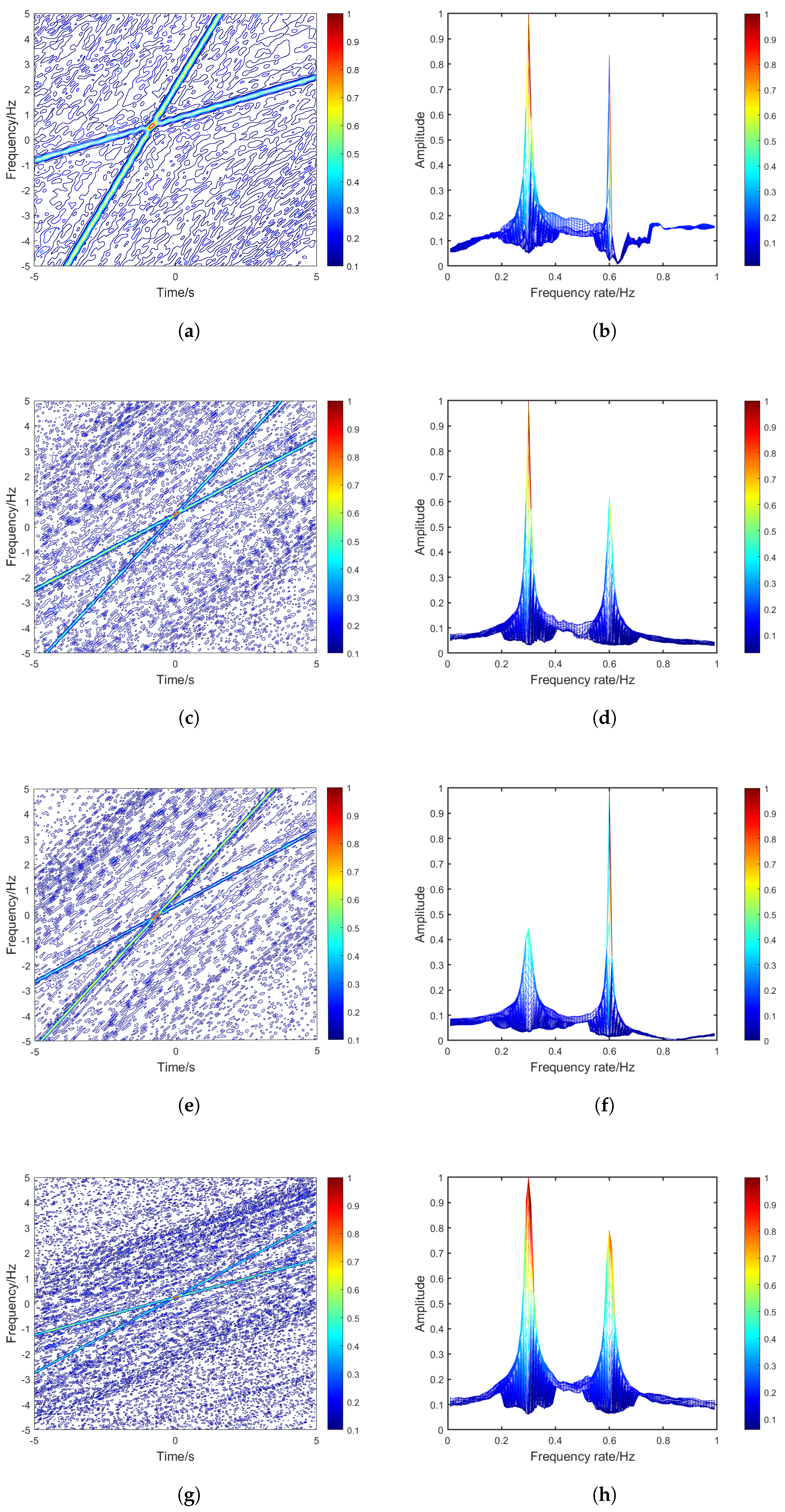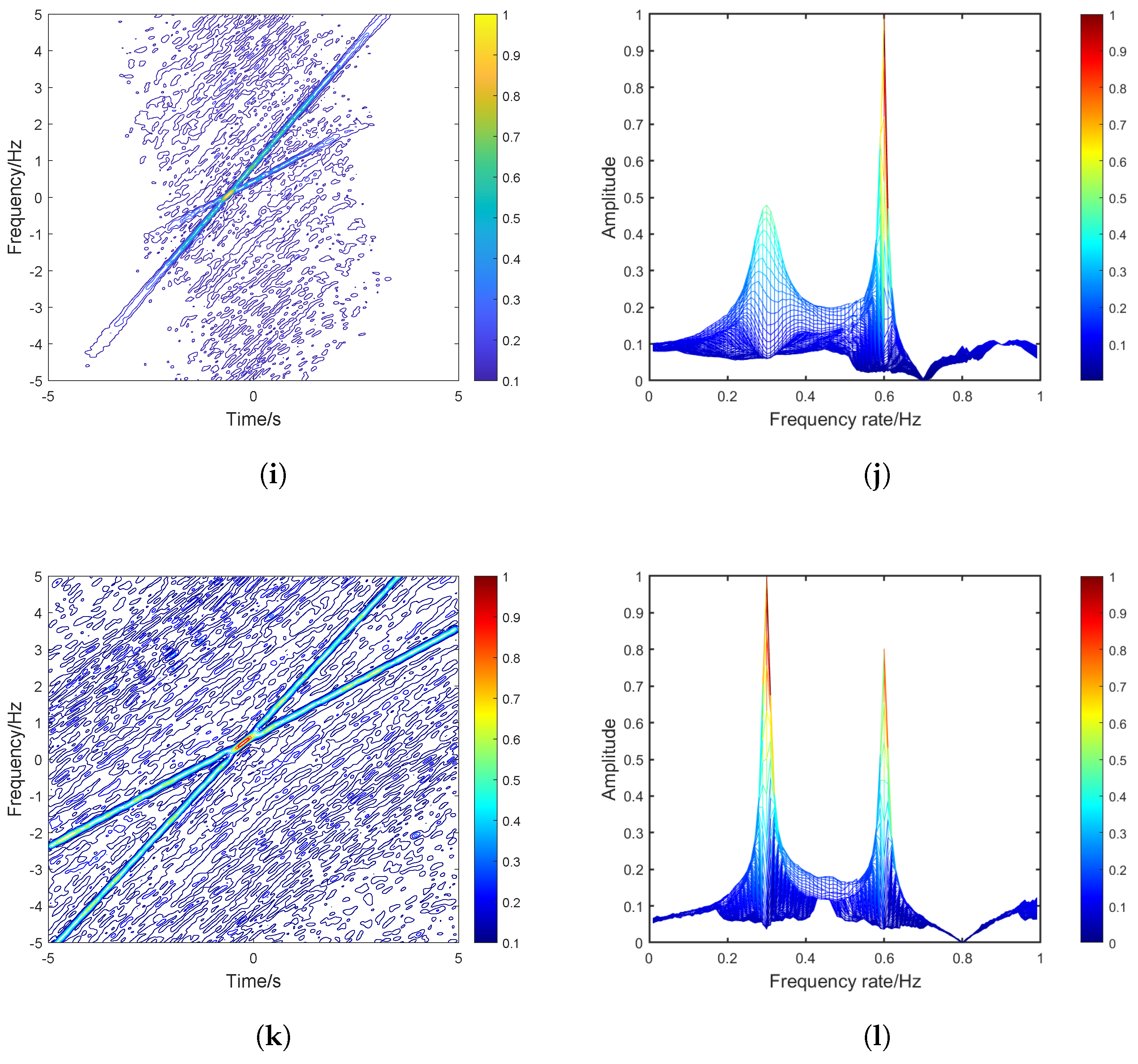Section 8 discusses some potential applications of the derived results. Section 9 draws a conclusion and presents future research directions.

2. FMKWD and Its Spreads

This section first rewrites the definition of the FMKWD as an integral form, and then proposes mathematical formulae for its spreads (time-FMKWD and FMT-FMKWD domains). It also collects many preliminary knowledge on spreads and spread matrices (time, FT, and FMT domains), covariance and covariance matrix, semiabsolute covariance and semiabsolute covariance matrix, and absolute covariance and the absolute covariance matrix.

Let ${\widehat{f}}_{{\mathbf{M}}_j}\left(\mathbf{u}\right)$ be the FMT of a function $f\left(\mathbf{x}\right)\in L^2\left({\mathbb{R}}^N\right)$ with the symplectic matrix ${\mathbf{M}}_j=\left(\begin{array}{cc}{\mathbf{A}}_j& {\mathbf{B}}_j\\ {\mathbf{C}}_j& {\mathbf{D}}_j\end{array}\right)$, $j=1,2$, and let a symplectic matrix $\mathbf{M}=\left(\begin{array}{cc}\mathbf{A}& \mathbf{B}\\ \mathbf{C}& \mathbf{D}\end{array}\right)$ with $\det \left(\mathbf{B}\right)\ne 0$ and a parameter matrix $\mathbf{K}=\mathrm{diag}\left(k_1,\cdots ,k_N\right)$, $k_n\in [0,1]$, $n=1,\cdots ,N$. The FMKWD of the function $f\left(\mathbf{x}\right)$ associated with the symplectic matrices ${\mathbf{M}}_1$, ${\mathbf{M}}_2$, $\mathbf{M}$ and the parameter matrix $\mathbf{K}$, as defined by (8), can be rewritten as follows:

$${\mathrm{W}}_f^{{\mathbf{M}}_1,{\mathbf{M}}_2,\mathbf{M};\mathbf{K}}(\mathbf{x},\mathbf{u})={\int }_{{\mathbb{R}}^N}{\widehat{f}}_{{\mathbf{M}}_1}\left(\mathbf{x}+\mathbf{y}\mathbf{K}\right)\overline{{\widehat{f}}_{{\mathbf{M}}_2}\left(\mathbf{x}-\mathbf{y}({\mathbf{I}}_N-\mathbf{K})\right)}{\mathcal{K}}_{\mathbf{M}}(\mathbf{u},\mathbf{y})\mathrm{d}\mathbf{y}.$$

(9)

It can be seen that one symplectic matrix has $N(2N+1)$ degrees of freedom [20], and then $3N(2N+1)$ degrees of freedom for three symplectic matrices ${\mathbf{M}}_1$, ${\mathbf{M}}_2$, $\mathbf{M}$. Moreover, the parameter matrix $\mathbf{K}$ has N degrees of freedom. The total degrees of freedom of FMKWD are therefore $2N(3N+2)$. As a result, the FMKWD includes as special cases some celebrated time-frequency distributions: the free metaplectic k-Wigner distribution (FMkWD), whose special cases also include the free metaplectic Rihaczek transform, free metaplectic Wigner distribution, and conjugate free metaplectic Rihaczek transform; the affine characteristic $\mathbf{K}$-Wigner distribution (ACKWD) and the N-dimensional affine characteristic k-Wigner distribution (N-D ACkWD), whose special cases also include the N-dimensional affine characteristic Rihaczek transform (N-D ACRT), N-D ACWD, and conjugate N-D ACRT; the kernel function $\mathbf{K}$-Wigner distribution (KFKWD) and the N-dimensional kernel function k-Wigner distribution (N-D KFkWD), whose special cases also include the N-dimensional kernel function Rihaczek transform (N-D KFRT), N-D KFWD, and conjugate N-D KFRT; the convolution representation $\mathbf{K}$-Wigner distribution (CRKWD) and the N-dimensional convolution representation k-Wigner distribution (N-D CRkWD), whose special cases also include the N-dimensional convolution representation Rihaczek transform (N-D CRRT), N-D CRWD, and conjugate N-D CRRT; the instantaneous cross-correlation function $\mathbf{K}$-Wigner distribution (ICFKWD) and the N-dimensional instantaneous cross-correlation function k-Wigner distribution (N-D ICFkWD), whose special cases also include the N-dimensional instantaneous cross-correlation function Rihaczek transform (N-D ICFRT), N-D ICFWD, and conjugate N-D ICFRT; and the $\mathbf{K}$-Wigner distribution and the N-dimensional k-Wigner distribution, whose special cases also include the N-dimensional Rihaczek transform, N-dimensional Wigner distribution, and conjugate N-dimensional Rihaczek transform. These distributions are summarized in

Table 1. Some special cases of the FMKWD.

Symplectic Matrices	Parameter Matrix			FMKWD
${\mathbf{M}}_1,{\mathbf{M}}_2,\mathbf{M}$	$\mathbf{K}=k{\mathbf{I}}_N$			FMkWD
	$\mathbf{0}$	${\displaystyle \frac{{\mathbf{I}}_N}{2}}$	${\mathbf{I}}_N$	Free metaplectic	Free metaplectic	Conjugate free metaplectic
				Rihaczek transform	Wigner distribution	Rihaczek transform
${\mathbf{M}}_1={\mathbf{M}}_2$,	$\mathbf{K}$			ACKWD
$\mathbf{M}=\left(\begin{array}{cc}\mathbf{0}& {\mathbf{I}}_N\\ -{\mathbf{I}}_N& \mathbf{0}\end{array}\right)$	$\mathbf{K}=k{\mathbf{I}}_N$			N-D ACkWD
	$\mathbf{0}$	${\displaystyle \frac{{\mathbf{I}}_N}{2}}$	${\mathbf{I}}_N$	N-D ACRT	N-D ACWD	Conjugate N-D ACRT
${\mathbf{M}}_1={\mathbf{M}}_2={\mathbf{I}}_{2N}$, $\mathbf{M}$	$\mathbf{K}$			KFKWD
	$\mathbf{K}=k{\mathbf{I}}_N$			N-D KFkWD
	$\mathbf{0}$	${\displaystyle \frac{{\mathbf{I}}_N}{2}}$	${\mathbf{I}}_N$	N-D KFRT	N-D KFWD	Conjugate N-D KFRT
${\mathbf{M}}_1=\left(\begin{array}{cc}{\mathbf{A}}_1& {\mathbf{B}}_1\\ {\mathbf{C}}_1& {\mathbf{D}}_1\end{array}\right)$,	$\mathbf{K}$			CRKWD
${\mathbf{M}}_2=\left(\begin{array}{cc}-{\mathbf{A}}_1& {\mathbf{B}}_1\\ {\mathbf{C}}_1& -{\mathbf{D}}_1\end{array}\right)$,	$\mathbf{K}=k{\mathbf{I}}_N$			N-D CRkWD
$\mathbf{M}=\left(\begin{array}{cc}{\displaystyle \frac{{\mathbf{D}}_1}{4}}& -{\mathbf{B}}_1\\ -{\mathbf{C}}_1& 4{\mathbf{A}}_1\end{array}\right)$	$\mathbf{0}$	${\displaystyle \frac{{\mathbf{I}}_N}{2}}$	${\mathbf{I}}_N$	N-D CRRT	N-D CRWD	Conjugate N-D CRRT
${\mathbf{M}}_1$, ${\mathbf{M}}_2={\mathbf{I}}_{2N}$, $\mathbf{M}$	$\mathbf{K}$			ICFKWD
	$\mathbf{K}=k{\mathbf{I}}_N$			N-D ICFkWD
	$\mathbf{0}$	${\displaystyle \frac{{\mathbf{I}}_N}{2}}$	${\mathbf{I}}_N$	N-D ICFRT	N-D ICFWD	Conjugate N-D ICFRT
${\mathbf{M}}_1={\mathbf{M}}_2={\mathbf{I}}_{2N}$,	$\mathbf{K}$			$\mathbf{K}$-Wigner distribution
$\mathbf{M}=\left(\begin{array}{cc}\mathbf{0}& {\mathbf{I}}_N\\ -{\mathbf{I}}_N& \mathbf{0}\end{array}\right)$	$\mathbf{K}=k{\mathbf{I}}_N$			N-dimensional k-Wigner distribution
	$\mathbf{0}$	${\displaystyle \frac{{\mathbf{I}}_N}{2}}$	${\mathbf{I}}_N$	N-dimensional	N-dimensional	Conjugate N-dimensional
				Rihaczek transform	Wigner distribution	Rihaczek transform

.

Remark 1

(Parseval’s relations of the FT and FMT). Let $\widehat{f}\left(\mathbf{w}\right)$ be the N-dimensional FT of $f\left(\mathbf{x}\right)$, and ${\widehat{f}}_{\mathbf{M}}\left(\mathbf{u}\right)$ be the FMT of $f\left(\mathbf{x}\right)$ with the symplectic matrix $\mathbf{M}=\left(\begin{array}{cc}\mathbf{A}& \mathbf{B}\\ \mathbf{C}& \mathbf{D}\end{array}\right)$. Assume that $f\left(\mathbf{x}\right)\in L^2\left({\mathbb{R}}^N\right)$. Then, there is ${\parallel f\parallel }_2={∥\widehat{f}∥}_2={∥{\widehat{f}}_{\mathbf{M}}∥}_2$.

Definition 7

(see [37], Definition 1.3). Let $\widehat{f}\left(\mathbf{w}\right)$ be the N-dimensional FT of $f\left(\mathbf{x}\right)$, ${\widehat{f}}_{\mathbf{M}}\left(\mathbf{u}\right)$ be the FMT of $f\left(\mathbf{x}\right)$ with the symplectic matrix $\mathbf{M}=\left(\begin{array}{cc}\mathbf{A}& \mathbf{B}\\ \mathbf{C}& \mathbf{D}\end{array}\right)$, and ${\mathrm{W}}_f^{{\mathbf{M}}_1,{\mathbf{M}}_2,\mathbf{M};\mathbf{K}}(\mathbf{x},\mathbf{u})$ be the FMKWD of $f\left(\mathbf{x}\right)$ associated with the symplectic matrices ${\mathbf{M}}_1=\left(\begin{array}{cc}{\mathbf{A}}_1& {\mathbf{B}}_1\\ {\mathbf{C}}_1& {\mathbf{D}}_1\end{array}\right)$, ${\mathbf{M}}_2=\left(\begin{array}{cc}{\mathbf{A}}_2& {\mathbf{B}}_2\\ {\mathbf{C}}_2& {\mathbf{D}}_2\end{array}\right)$, $\mathbf{M}=\left(\begin{array}{cc}\mathbf{A}& \mathbf{B}\\ \mathbf{C}& \mathbf{D}\end{array}\right)$ and the parameter matrix $\mathbf{K}=\mathrm{diag}\left(k_1,\cdots ,k_N\right)$. Assume that $f\left(\mathbf{x}\right),\mathbf{x}f\left(\mathbf{x}\right)$, $\mathbf{w}\widehat{f}\left(\mathbf{w}\right),\mathbf{u}{\widehat{f}}_{\mathbf{M}}\left(\mathbf{u}\right)\in L^2\left({\mathbb{R}}^N\right)$.

(i) Spread in the time domain:

$$\mathrm{\Delta }{\mathbf{x}}^2={\displaystyle \frac{{\int }_{{\mathbb{R}}^N}{∥\mathbf{x}-{\mathbf{x}}^0∥}^2{\left|f\left(\mathbf{x}\right)\right|}^2\mathrm{d}\mathbf{x}}{{\parallel f\parallel }_2^2}},$$

(10)

where the moment vector in the time domain:

$${\mathbf{x}}^0=\left(x_1^0,\cdots ,x_N^0\right)={\displaystyle \frac{{\int }_{{\mathbb{R}}^N}\mathbf{x}{\left|f\left(\mathbf{x}\right)\right|}^2\mathrm{d}\mathbf{x}}{{\parallel f\parallel }_2^2}}.$$

(11)

(ii) Spread in the FT domain:

$$\mathrm{\Delta }{\mathbf{w}}^2={\displaystyle \frac{{\int }_{{\mathbb{R}}^N}{∥\mathbf{w}-{\mathbf{w}}^0∥}^2{\left|\widehat{f}\left(\mathbf{w}\right)\right|}^2\mathrm{d}\mathbf{w}}{{\parallel f\parallel }_2^2}},$$

(12)

where the moment vector in the FT domain:

$${\mathbf{w}}^0=\left({\omega }_1^0,\cdots ,{\omega }_N^0\right)={\displaystyle \frac{{\int }_{{\mathbb{R}}^N}\mathbf{w}{\left|\widehat{f}\left(\mathbf{w}\right)\right|}^2\mathrm{d}\mathbf{w}}{{\parallel f\parallel }_2^2}}.$$

(13)

(iii) Spread in the FMT domain:

$$\mathrm{\Delta }{\mathbf{u}}_{\mathbf{M}}^2={\displaystyle \frac{{\int }_{{\mathbb{R}}^N}{∥\mathbf{u}-{\mathbf{u}}_{\mathbf{M}}^0∥}^2{\left|{\widehat{f}}_{\mathbf{M}}\left(\mathbf{u}\right)\right|}^2\mathrm{d}\mathbf{u}}{{\parallel f\parallel }_2^2}},$$

(14)

where the moment vector in the FMT domain:

$${\mathbf{u}}_{\mathbf{M}}^0=\left(u_{\mathbf{M};1}^0,\cdots ,u_{\mathbf{M};N}^0\right)={\displaystyle \frac{{\int }_{{\mathbb{R}}^N}\mathbf{u}{\left|{\widehat{f}}_{\mathbf{M}}\left(\mathbf{u}\right)\right|}^2\mathrm{d}\mathbf{u}}{{\parallel f\parallel }_2^2}}.$$

(15)

(iv) Spread in the time-FMKWD domain:

$$\mathrm{\Delta }{\mathbf{x}}_{{\mathbf{M}}_1,{\mathbf{M}}_2,\mathbf{M};\mathbf{K}}^2={\displaystyle \frac{{\int \int }_{{\mathbb{R}}^{N\times N}}{∥\mathbf{x}-{\mathbf{x}}_{{\mathbf{M}}_1,{\mathbf{M}}_2,\mathbf{M};\mathbf{K}}^0∥}^2{\left|{\mathrm{W}}_f^{{\mathbf{M}}_1,{\mathbf{M}}_2,\mathbf{M};\mathbf{K}}(\mathbf{x},\mathbf{u})\right|}^2\mathrm{d}\mathbf{x}\mathrm{d}\mathbf{u}}{{∥{\mathrm{W}}_f^{{\mathbf{M}}_1,{\mathbf{M}}_2,\mathbf{M};\mathbf{K}}∥}_2^2}},$$

(16)

where the moment vector in the time-FMKWD domain:

$${\mathbf{x}}_{{\mathbf{M}}_1,{\mathbf{M}}_2,\mathbf{M};\mathbf{K}}^0=\left(x_{{\mathbf{M}}_1,{\mathbf{M}}_2,\mathbf{M};\mathbf{K};1}^0,\cdots ,x_{{\mathbf{M}}_1,{\mathbf{M}}_2,\mathbf{M};\mathbf{K};N}^0\right)={\displaystyle \frac{{\int \int }_{{\mathbb{R}}^{N\times N}}\mathbf{x}{\left|{\mathrm{W}}_f^{{\mathbf{M}}_1,{\mathbf{M}}_2,\mathbf{M};\mathbf{K}}(\mathbf{x},\mathbf{u})\right|}^2\mathrm{d}\mathbf{x}\mathrm{d}\mathbf{u}}{{∥{\mathrm{W}}_f^{{\mathbf{M}}_1,{\mathbf{M}}_2,\mathbf{M};\mathbf{K}}∥}_2^2}}.$$

(17)

(v) Spread in the FMT-FMKWD domain:

$$\mathrm{\Delta }{\mathbf{u}}_{{\mathbf{M}}_1,{\mathbf{M}}_2,\mathbf{M};\mathbf{K}}^2={\displaystyle \frac{{\int \int }_{{\mathbb{R}}^{N\times N}}{∥\mathbf{u}-{\mathbf{u}}_{{\mathbf{M}}_1,{\mathbf{M}}_2,\mathbf{M};\mathbf{K}}^0∥}^2{\left|{\mathrm{W}}_f^{{\mathbf{M}}_1,{\mathbf{M}}_2,\mathbf{M};\mathbf{K}}(\mathbf{x},\mathbf{u})\right|}^2\mathrm{d}\mathbf{x}\mathrm{d}\mathbf{u}}{{∥{\mathrm{W}}_f^{{\mathbf{M}}_1,{\mathbf{M}}_2,\mathbf{M};\mathbf{K}}∥}_2^2}},$$

(18)

where the moment vector in the FMT-FMKWD domain:

$${\mathbf{u}}_{{\mathbf{M}}_1,{\mathbf{M}}_2,\mathbf{M};\mathbf{K}}^0=\left(u_{{\mathbf{M}}_1,{\mathbf{M}}_2,\mathbf{M};\mathbf{K};1}^0,\cdots ,u_{{\mathbf{M}}_1,{\mathbf{M}}_2,\mathbf{M};\mathbf{K};N}^0\right)={\displaystyle \frac{{\int \int }_{{\mathbb{R}}^{N\times N}}\mathbf{u}{\left|{\mathrm{W}}_f^{{\mathbf{M}}_1,{\mathbf{M}}_2,\mathbf{M};\mathbf{K}}(\mathbf{x},\mathbf{u})\right|}^2\mathrm{d}\mathbf{x}\mathrm{d}\mathbf{u}}{{∥{\mathrm{W}}_f^{{\mathbf{M}}_1,{\mathbf{M}}_2,\mathbf{M};\mathbf{K}}∥}_2^2}}.$$

(19)

Definition 8

(see [37], Definitions 1.3 and 1.4). Let $\widehat{f}\left(\mathbf{w}\right)$ be the N-dimensional FT of $f\left(\mathbf{x}\right)=\lambda \left(\mathbf{x}\right){\mathrm{e}}^{2\pi \mathrm{i}\phi \left(\mathbf{x}\right)}\in L^2\left({\mathbb{R}}^N\right)$. Assume that for any $1\le n\le N$, the classical partial derivatives ${\displaystyle \frac{\partial \lambda }{\partial x_n}},{\displaystyle \frac{\partial \phi }{\partial x_n}},{\displaystyle \frac{\partial f}{\partial x_n}}$ exist at any point $\mathbf{x}\in {\mathbb{R}}^N$, and $\mathbf{x}f\left(\mathbf{x}\right),\mathbf{w}\widehat{f}\left(\mathbf{w}\right)\in L^2\left({\mathbb{R}}^N\right)$.

(i) Covariance matrix in the time-frequency domain:

$${\mathrm{Cov}}_{\mathbf{X},\mathbf{W}}=\left(\begin{array}{c}{\mathrm{Cov}}_{\mathbf{x},\mathbf{w}}^{n,m}\end{array}\right)={\displaystyle \frac{{\int }_{{\mathbb{R}}^N}{\left(\mathbf{x}-{\mathbf{x}}^0\right)}^{\mathrm{T}}\left({\nabla }_{\mathbf{x}}\phi -{\mathbf{w}}^0\right){\lambda }^2\left(\mathbf{x}\right)\mathrm{d}\mathbf{x}}{{\parallel f\parallel }_2^2}}.$$

(20)

(ii) Covariance in the time-frequency domain:

$${\mathrm{Cov}}_{\mathbf{x},\mathbf{w}}=\mathrm{tr}\left({\mathrm{Cov}}_{\mathbf{X},\mathbf{W}}\right)={\displaystyle \frac{{\int }_{{\mathbb{R}}^N}\left(\mathbf{x}-{\mathbf{x}}^0\right){\left({\nabla }_{\mathbf{x}}\phi -{\mathbf{w}}^0\right)}^{\mathrm{T}}{\lambda }^2\left(\mathbf{x}\right)\mathrm{d}\mathbf{x}}{{\parallel f\parallel }_2^2}}.$$

(21)

(iii) Semiabsolute covariance matrix in the time-frequency domain:

$${\left|\mathrm{Cov}\right|}_{\mathbf{X},\mathbf{W}}=\left(\begin{array}{c}{\left|\mathrm{Cov}\right|}_{\mathbf{x},\mathbf{w}}^{n,m}\end{array}\right)={\displaystyle \frac{\left|{\int }_{{\mathbb{R}}^N}{\left(\mathbf{x}-{\mathbf{x}}^0\right)}^{\mathrm{T}}\left({\nabla }_{\mathbf{x}}\phi -{\mathbf{w}}^0\right){\lambda }^2\left(\mathbf{x}\right)\mathrm{d}\mathbf{x}\right|}{{\parallel f\parallel }_2^2}}.$$

(22)

(iv) Semiabsolute covariance in the time-frequency domain:

$${\left|\mathrm{Cov}\right|}_{\mathbf{x},\mathbf{w}}={\mathrm{tr}\left(\right|\mathrm{Cov}|}_{\mathbf{X},\mathbf{W}})={\displaystyle \frac{{\displaystyle \sum _{n=1}^N}\left|{\int }_{{\mathbb{R}}^N}\left(x_n-x_n^0\right)\left(\frac{\partial \phi }{\partial x_n}-{\omega }_n^0\right){\lambda }^2\left(\mathbf{x}\right)\mathrm{d}\mathbf{x}\right|}{{\parallel f\parallel }_2^2}}.$$

(23)

(v) Absolute covariance matrix in the time-frequency domain:

$${\mathrm{COV}}_{\mathbf{X},\mathbf{W}}=\left(\begin{array}{c}{\mathrm{COV}}_{\mathbf{x},\mathbf{w}}^{n,m}\end{array}\right)={\displaystyle \frac{{\int }_{{\mathbb{R}}^N}{\left|\mathbf{x}-{\mathbf{x}}^0\right|}^{\mathrm{T}}\left|{\nabla }_{\mathbf{x}}\phi -{\mathbf{w}}^0\right|{\lambda }^2\left(\mathbf{x}\right)\mathrm{d}\mathbf{x}}{{\parallel f\parallel }_2^2}}.$$

(24)

(vi) Absolute covariance in the time-frequency domain:

$${\mathrm{COV}}_{\mathbf{x},\mathbf{w}}=\mathrm{tr}\left({\mathrm{COV}}_{\mathbf{X},\mathbf{W}}\right)={\displaystyle \frac{{\int }_{{\mathbb{R}}^N}\left|\mathbf{x}-{\mathbf{x}}^0\right|{\left|{\nabla }_{\mathbf{x}}\phi -{\mathbf{w}}^0\right|}^{\mathrm{T}}{\lambda }^2\left(\mathbf{x}\right)\mathrm{d}\mathbf{x}}{{\parallel f\parallel }_2^2}}.$$

(25)

Definition 9

(see [37], Definition 1.4). Let $\widehat{f}\left(\mathbf{w}\right)$ be the N-dimensional FT of $f\left(\mathbf{x}\right)$, and ${\widehat{f}}_{\mathbf{M}}\left(\mathbf{u}\right)$ be the FMT of $f\left(\mathbf{x}\right)$ with the symplectic matrix $\mathbf{M}=\left(\begin{array}{cc}\mathbf{A}& \mathbf{B}\\ \mathbf{C}& \mathbf{D}\end{array}\right)$. Assume that $f\left(\mathbf{x}\right),\mathbf{x}f\left(\mathbf{x}\right),\mathbf{w}\widehat{f}\left(\mathbf{w}\right)$, $\mathbf{u}{\widehat{f}}_{\mathbf{M}}\left(\mathbf{u}\right)\in L^2\left({\mathbb{R}}^N\right)$.

(i) Spread matrix in the time domain:

$$\mathbf{X}=\left(\begin{array}{c}\mathrm{\Delta }{\mathbf{x}}_{n,m}^2\end{array}\right)={\displaystyle \frac{{\int }_{{\mathbb{R}}^N}{\left(\mathbf{x}-{\mathbf{x}}^0\right)}^{\mathrm{T}}\left(\mathbf{x}-{\mathbf{x}}^0\right){\left|f\left(\mathbf{x}\right)\right|}^2\mathrm{d}\mathbf{x}}{{\parallel f\parallel }_2^2}}.$$

(26)

(ii) Spread matrix in the FT domain:

$$\mathbf{W}=\left(\begin{array}{c}\mathrm{\Delta }{\mathbf{w}}_{n,m}^2\end{array}\right)={\displaystyle \frac{{\int }_{{\mathbb{R}}^N}{\left(\mathbf{w}-{\mathbf{w}}^0\right)}^{\mathrm{T}}\left(\mathbf{w}-{\mathbf{w}}^0\right){\left|\widehat{f}\left(\mathbf{w}\right)\right|}^2\mathrm{d}\mathbf{w}}{{\parallel f\parallel }_2^2}}.$$

(27)

(iii) Spread matrix in the FMT domain:

$${\mathbf{U}}_{\mathbf{M}}=\left(\begin{array}{c}\mathrm{\Delta }{\mathbf{u}}_{\mathbf{M};n,m}^2\end{array}\right)={\displaystyle \frac{{\int }_{{\mathbb{R}}^N}{\left(\mathbf{u}-{\mathbf{u}}_{\mathbf{M}}^0\right)}^{\mathrm{T}}\left(\mathbf{u}-{\mathbf{u}}_{\mathbf{M}}^0\right){\left|{\widehat{f}}_{\mathbf{M}}\left(\mathbf{u}\right)\right|}^2\mathrm{d}\mathbf{u}}{{\parallel f\parallel }_2^2}}.$$

(28)

Remark 2.

There are relations $\mathrm{\Delta }{\mathbf{x}}^2=\mathrm{tr}\left(\mathbf{X}\right)$, $\mathrm{\Delta }{\mathbf{w}}^2=\mathrm{tr}\left(\mathbf{W}\right)$ and $\mathrm{\Delta }{\mathbf{u}}_{\mathbf{M}}^2=\mathrm{tr}\left({\mathbf{U}}_{\mathbf{M}}\right)$.

3. Uncertainty Product in FMKWD Domains

This section first obtains Parseval’s relation of the FMKWD and a mathematical formula for the FMKWD in the FMT domain. It then discloses relations between spreads in time-FMKWD (FMT-FMKWD) and FMT domains, and finally combines them to formulate an equivalence relation between the uncertainty product in time-FMKWD and FMT-FMKWD domains and those in two FMT domains.

Lemma 1

(Parseval’s relation of the FMKWD). Let ${\mathrm{W}}_f^{{\mathbf{M}}_1,{\mathbf{M}}_2,\mathbf{M};\mathbf{K}}(\mathbf{x},\mathbf{u})$ be the FMKWD of $f\left(\mathbf{x}\right)\in L^2\left({\mathbb{R}}^N\right)$ associated with the symplectic matrices ${\mathbf{M}}_1=\left(\begin{array}{cc}{\mathbf{A}}_1& {\mathbf{B}}_1\\ {\mathbf{C}}_1& {\mathbf{D}}_1\end{array}\right)$, ${\mathbf{M}}_2=\left(\begin{array}{cc}{\mathbf{A}}_2& {\mathbf{B}}_2\\ {\mathbf{C}}_2& {\mathbf{D}}_2\end{array}\right)$, $\mathbf{M}=\left(\begin{array}{cc}\mathbf{A}& \mathbf{B}\\ \mathbf{C}& \mathbf{D}\end{array}\right)$ and the parameter matrix $\mathbf{K}=\mathrm{diag}\left(k_1,\cdots ,k_N\right)$. Then, there is ${∥{\mathrm{W}}_f^{{\mathbf{M}}_1,{\mathbf{M}}_2,\mathbf{M};\mathbf{K}}∥}_2={\parallel f\parallel }_2^2$.

Proof. 

From (9), there is

$$\begin{array}{cc}\hfill & {∥{\mathrm{W}}_f^{{\mathbf{M}}_1,{\mathbf{M}}_2,\mathbf{M};\mathbf{K}}∥}_2^2\hfill \\ \hfill =& {\int \int }_{{\mathbb{R}}^{N\times N}}{\left|{\mathrm{W}}_f^{{\mathbf{M}}_1,{\mathbf{M}}_2,\mathbf{M};\mathbf{K}}(\mathbf{x},\mathbf{u})\right|}^2\mathrm{d}\mathbf{x}\mathrm{d}\mathbf{u}\hfill \\ \hfill =& {\int \int \int }_{{\mathbb{R}}^{N\times N\times N}}{\widehat{f}}_{{\mathbf{M}}_1}\left(\mathbf{x}+\mathbf{y}\mathbf{K}\right)\overline{{\widehat{f}}_{{\mathbf{M}}_2}\left(\mathbf{x}-\mathbf{y}({\mathbf{I}}_N-\mathbf{K})\right)}\overline{{\widehat{f}}_{{\mathbf{M}}_1}\left(\mathbf{x}+\mathbf{z}\mathbf{K}\right)}{\widehat{f}}_{{\mathbf{M}}_2}\left(\mathbf{x}-\mathbf{z}({\mathbf{I}}_N-\mathbf{K})\right)\hfill \\ \hfill & \times \left({\int }_{{\mathbb{R}}^N}{\mathcal{K}}_{\mathbf{M}}(\mathbf{u},\mathbf{y})\overline{{\mathcal{K}}_{\mathbf{M}}(\mathbf{u},\mathbf{z})}\mathrm{d}\mathbf{u}\right)\mathrm{d}\mathbf{x}\mathrm{d}\mathbf{y}\mathrm{d}\mathbf{z}.\hfill \end{array}$$

(29)

Thanks to

$${\int }_{{\mathbb{R}}^N}{\mathcal{K}}_{\mathbf{M}}(\mathbf{u},\mathbf{y})\overline{{\mathcal{K}}_{\mathbf{M}}(\mathbf{u},\mathbf{z})}\mathrm{d}\mathbf{u}={\mathrm{e}}^{\pi \mathrm{i}\left(\mathbf{y}{\mathbf{B}}^{-1}\mathbf{A}{\mathbf{y}}^{\mathrm{T}}-\mathbf{z}{\mathbf{B}}^{-1}\mathbf{A}{\mathbf{z}}^{\mathrm{T}}\right)}\delta (\mathbf{y}-\mathbf{z}),$$

(30)

Equation (29) becomes

$$\begin{array}{cc}\hfill & {∥{\mathrm{W}}_f^{{\mathbf{M}}_1,{\mathbf{M}}_2,\mathbf{M};\mathbf{K}}∥}_2^2\hfill \\ \hfill =& {\int \int }_{{\mathbb{R}}^{N\times N}}{\widehat{f}}_{{\mathbf{M}}_1}\left(\mathbf{x}+\mathbf{y}\mathbf{K}\right)\overline{{\widehat{f}}_{{\mathbf{M}}_2}\left(\mathbf{x}-\mathbf{y}({\mathbf{I}}_N-\mathbf{K})\right)}\hfill \\ \hfill & \times \left({\int }_{{\mathbb{R}}^N}\overline{{\widehat{f}}_{{\mathbf{M}}_1}\left(\mathbf{x}+\mathbf{z}\mathbf{K}\right)}{\widehat{f}}_{{\mathbf{M}}_2}\left(\mathbf{x}-\mathbf{z}({\mathbf{I}}_N-\mathbf{K})\right){\mathrm{e}}^{\pi \mathrm{i}\left(\mathbf{y}{\mathbf{B}}^{-1}\mathbf{A}{\mathbf{y}}^{\mathrm{T}}-\mathbf{z}{\mathbf{B}}^{-1}\mathbf{A}{\mathbf{z}}^{\mathrm{T}}\right)}\delta (\mathbf{y}-\mathbf{z})\mathrm{d}\mathbf{z}\right)\mathrm{d}\mathbf{x}\mathrm{d}\mathbf{y}\hfill \\ \hfill =& {\int \int }_{{\mathbb{R}}^{N\times N}}{\left|{\widehat{f}}_{{\mathbf{M}}_1}\left(\mathbf{x}+\mathbf{y}\mathbf{K}\right)\right|}^2{\left|{\widehat{f}}_{{\mathbf{M}}_2}\left(\mathbf{x}-\mathbf{y}({\mathbf{I}}_N-\mathbf{K})\right)\right|}^2\mathrm{d}\mathbf{x}\mathrm{d}\mathbf{y}.\hfill \end{array}$$

(31)

By making the change of variables $\mathbf{x}=\mathbf{u}({\mathbf{I}}_N-\mathbf{K})+\mathbf{v}\mathbf{K}$ and $\mathbf{y}=\mathbf{u}-\mathbf{v}$, there is

$$\begin{array}{cc}\hfill {∥{\mathrm{W}}_f^{{\mathbf{M}}_1,{\mathbf{M}}_2,\mathbf{M};\mathbf{K}}∥}_2^2=& {\int }_{{\mathbb{R}}^N}{\left|{\widehat{f}}_{{\mathbf{M}}_1}\left(\mathbf{u}\right)\right|}^2\mathrm{d}\mathbf{u}{\int }_{{\mathbb{R}}^N}{\left|{\widehat{f}}_{{\mathbf{M}}_2}\left(\mathbf{v}\right)\right|}^2\mathrm{d}\mathbf{v}\hfill \\ \hfill =& {∥{\widehat{f}}_{{\mathbf{M}}_1}∥}_2^2{∥{\widehat{f}}_{{\mathbf{M}}_2}∥}_2^2.\hfill \end{array}$$

(32)

From Remark 1, the required result follows ${∥{\mathrm{W}}_f^{{\mathbf{M}}_1,{\mathbf{M}}_2,\mathbf{M};\mathbf{K}}∥}_2^2={\parallel f\parallel }_2^4$. □

Lemma 2.

Let ${\mathrm{W}}_f^{{\mathbf{M}}_1,{\mathbf{M}}_2,\mathbf{M};\mathbf{K}}(\mathbf{x},\mathbf{u})$ be the FMKWD of $f\left(\mathbf{x}\right)$ associated with the symplectic matrices ${\mathbf{M}}_1=\left(\begin{array}{cc}{\mathbf{A}}_1& {\mathbf{B}}_1\\ {\mathbf{C}}_1& {\mathbf{D}}_1\end{array}\right)$, ${\mathbf{M}}_2=\left(\begin{array}{cc}{\mathbf{A}}_2& {\mathbf{B}}_2\\ {\mathbf{C}}_2& {\mathbf{D}}_2\end{array}\right)$, $\mathbf{M}=\left(\begin{array}{cc}\mathbf{A}& \mathbf{B}\\ \mathbf{C}& \mathbf{D}\end{array}\right)$ and the parameter matrix $\mathbf{K}=\mathrm{diag}\left(k_1,\cdots ,k_N\right)$, where $k_n\in (0,1)$, $n=1,\cdots ,N$, and ${\widehat{f}}_{{\check{\mathbf{M}}}_{{\mathbf{K}}_1}{\mathbf{M}}_1}\left(\mathbf{u}\right)$ and ${\widehat{f}}_{{\breve{\mathbf{M}}}_{{\mathbf{K}}_2}{\mathbf{M}}_2}\left(\mathbf{u}\right)$ be the FMTs of $f\left(\mathbf{x}\right)$ with the symplectic matrices ${\check{\mathbf{M}}}_{{\mathbf{K}}_1}{\mathbf{M}}_1$ and ${\breve{\mathbf{M}}}_{{\mathbf{K}}_2}{\mathbf{M}}_2$, respectively, where the symplectic matrices ${\check{\mathbf{M}}}_{{\mathbf{K}}_1}=\left(\begin{array}{cc}\mathbf{A}& \mathbf{B}{\mathbf{K}}_1\\ \mathbf{C}{\mathbf{K}}_1^{-1}& \mathbf{D}\end{array}\right)$ and ${\breve{\mathbf{M}}}_{{\mathbf{K}}_2}=\left(\begin{array}{cc}\mathbf{A}& -\mathbf{B}{\mathbf{K}}_2\\ -\mathbf{C}{\mathbf{K}}_2^{-1}& \mathbf{D}\end{array}\right)$, and where ${\mathbf{K}}_1=\mathbf{K}$ and ${\mathbf{K}}_2={\mathbf{I}}_N-\mathbf{K}$. Assume that $f\left(\mathbf{x}\right)\in L^2\left({\mathbb{R}}^N\right)$. Then, the FMKWD can be rewritten in the FMT domain as

$$\begin{array}{cc}\hfill {\mathrm{W}}_f^{{\mathbf{M}}_1,{\mathbf{M}}_2,\mathbf{M};\mathbf{K}}(\mathbf{x},\mathbf{u})=& {\displaystyle \frac{{\mathrm{e}}^{-\pi \mathrm{i}\mathbf{x}{\mathbf{K}}_1^{-1}{\mathbf{K}}_2^{-1}{\mathbf{B}}^{-1}\mathbf{A}{\mathbf{x}}^{\mathrm{T}}}{\mathrm{e}}^{\pi \mathrm{i}\mathbf{u}\mathbf{D}{\mathbf{B}}^{-1}{\mathbf{u}}^{\mathrm{T}}}}{\sqrt{{(-1)}^{N+1}\det \left(\mathbf{B}\right){\displaystyle \prod _{n=1}^N}{k}_n(1-k_n)}}}{\int }_{{\mathbb{R}}^N}{\widehat{f}}_{{\check{\mathbf{M}}}_{{\mathbf{K}}_1}{\mathbf{M}}_1}\left(\mathbf{v}\right)\overline{{\widehat{f}}_{{\breve{\mathbf{M}}}_{{\mathbf{K}}_2}{\mathbf{M}}_2}(\mathbf{v}-\mathbf{u})}\hfill \\ \hfill & \times {\mathrm{e}}^{-\pi \mathrm{i}(\mathbf{v}\mathbf{D}-2\mathbf{x}){\mathbf{K}}_1^{-1}{\mathbf{B}}^{-1}{\mathbf{v}}^{\mathrm{T}}}{\mathrm{e}}^{-\pi \mathrm{i}[(\mathbf{v}-\mathbf{u})\mathbf{D}-2\mathbf{x}]{\mathbf{K}}_2^{-1}{\mathbf{B}}^{-1}{(\mathbf{v}-\mathbf{u})}^{\mathrm{T}}}\mathrm{d}\mathbf{v}.\hfill \end{array}$$

(33)

Proof. 

Thanks to the FMT’s additive and inverse formulae, there are

$${\widehat{f}}_{{\mathbf{M}}_1}\left(\mathbf{x}+\mathbf{y}{\mathbf{K}}_1\right)={\int }_{{\mathbb{R}}^N}{\widehat{f}}_{{\check{\mathbf{M}}}_{{\mathbf{K}}_1}{\mathbf{M}}_1}\left(\mathbf{v}\right){\mathcal{K}}_{{\check{\mathbf{M}}}_{{\mathbf{K}}_1}^{-1}}\left(\mathbf{x}+\mathbf{y}{\mathbf{K}}_1,\mathbf{v}\right)\mathrm{d}\mathbf{v}$$

(34)

and

$$\overline{{\widehat{f}}_{{\mathbf{M}}_2}\left(\mathbf{x}-\mathbf{y}{\mathbf{K}}_2\right)}={\int }_{{\mathbb{R}}^N}\overline{{\widehat{f}}_{{\breve{\mathbf{M}}}_{{\mathbf{K}}_2}{\mathbf{M}}_2}\left(\mathbf{w}\right)}\overline{{\mathcal{K}}_{{\breve{\mathbf{M}}}_{{\mathbf{K}}_2}^{-1}}\left(\mathbf{x}-\mathbf{y}{\mathbf{K}}_2,\mathbf{w}\right)}\mathrm{d}\mathbf{w},$$

(35)

where the symplectic matrices ${\check{\mathbf{M}}}_{{\mathbf{K}}_1}^{-1}=\left(\begin{array}{cc}{\mathbf{D}}^{\mathrm{T}}& -{\mathbf{K}}_1{\mathbf{B}}^{\mathrm{T}}\\ -{\mathbf{K}}_1^{-1}{\mathbf{C}}^{\mathrm{T}}& {\mathbf{A}}^{\mathrm{T}}\end{array}\right)$ and ${\breve{\mathbf{M}}}_{{\mathbf{K}}_2}^{-1}=\left(\begin{array}{cc}{\mathbf{D}}^{\mathrm{T}}& {\mathbf{K}}_2{\mathbf{B}}^{\mathrm{T}}\\ {\mathbf{K}}_2^{-1}{\mathbf{C}}^{\mathrm{T}}& {\mathbf{A}}^{\mathrm{T}}\end{array}\right)$.

Substituting (34) and (35) into the definition of FMKWD gives

$$\begin{array}{cc}\hfill & {\mathrm{W}}_f^{{\mathbf{M}}_1,{\mathbf{M}}_2,\mathbf{M};\mathbf{K}}(\mathbf{x},\mathbf{u})\hfill \\ \hfill =& {\int \int \int }_{{\mathbb{R}}^{N\times N\times N}}{\widehat{f}}_{{\check{\mathbf{M}}}_{{\mathbf{K}}_1}{\mathbf{M}}_1}\left(\mathbf{v}\right)\overline{{\widehat{f}}_{{\breve{\mathbf{M}}}_{{\mathbf{K}}_2}{\mathbf{M}}_2}\left(\mathbf{w}\right)}\hfill \\ \hfill & \times {\mathcal{K}}_{\mathbf{M}}(\mathbf{u},\mathbf{y}){\mathcal{K}}_{{\check{\mathbf{M}}}_{{\mathbf{K}}_1}^{-1}}\left(\mathbf{x}+\mathbf{y}{\mathbf{K}}_1,\mathbf{v}\right)\overline{{\mathcal{K}}_{{\breve{\mathbf{M}}}_{{\mathbf{K}}_2}^{-1}}\left(\mathbf{x}-\mathbf{y}{\mathbf{K}}_2,\mathbf{w}\right)}\mathrm{d}\mathbf{v}\mathrm{d}\mathbf{w}\mathrm{d}\mathbf{y}\hfill \\ \hfill =& {\displaystyle \frac{{\mathrm{e}}^{-\pi \mathrm{i}\mathbf{x}\left({\mathbf{K}}_1^{-1}+{\mathbf{K}}_2^{-1}\right){\mathbf{B}}^{-1}\mathbf{A}{\mathbf{x}}^{\mathrm{T}}}{\mathrm{e}}^{\pi \mathrm{i}\mathbf{u}\mathbf{D}{\mathbf{B}}^{-1}{\mathbf{u}}^{\mathrm{T}}}}{\left|\det \left(\mathbf{B}\right)\right|\sqrt{{(-1)}^{N+1}\det \left(\mathbf{B}\right){\displaystyle \prod _{n=1}^N}{k}_n(1-k_n)}}}\hfill \\ \hfill & \times {\int \int }_{{\mathbb{R}}^{N\times N}}{\widehat{f}}_{{\check{\mathbf{M}}}_{{\mathbf{K}}_1}{\mathbf{M}}_1}\left(\mathbf{v}\right)\overline{{\widehat{f}}_{{\breve{\mathbf{M}}}_{{\mathbf{K}}_2}{\mathbf{M}}_2}\left(\mathbf{w}\right)}{\mathrm{e}}^{-\pi \mathrm{i}(\mathbf{v}\mathbf{D}-2\mathbf{x}){\mathbf{K}}_1^{-1}{\mathbf{B}}^{-1}{\mathbf{v}}^{\mathrm{T}}}{\mathrm{e}}^{-\pi \mathrm{i}(\mathbf{w}\mathbf{D}-2\mathbf{x}){\mathbf{K}}_2^{-1}{\mathbf{B}}^{-1}{\mathbf{w}}^{\mathrm{T}}}\hfill \\ \hfill & \times \left({\int }_{{\mathbb{R}}^N}{\mathrm{e}}^{-\pi \mathrm{i}\mathbf{x}\left({\mathbf{K}}_1^{-1}{\mathbf{B}}^{-1}\mathbf{A}{\mathbf{K}}_1-{\mathbf{K}}_2^{-1}{\mathbf{B}}^{-1}\mathbf{A}{\mathbf{K}}_2\right){\mathbf{y}}^{\mathrm{T}}}{\mathrm{e}}^{-2\pi \mathrm{i}\mathbf{y}{\mathbf{B}}^{-1}{(\mathbf{u}+\mathbf{w}-\mathbf{v})}^{\mathrm{T}}}\mathrm{d}\mathbf{y}\right)\mathrm{d}\mathbf{v}\mathrm{d}\mathbf{w}.\hfill \end{array}$$

(36)

The symplectic matrices $\mathbf{M}=\left(\begin{array}{cc}\mathbf{A}& \mathbf{B}\\ \mathbf{C}& \mathbf{D}\end{array}\right)$ and ${\check{\mathbf{M}}}_{{\mathbf{K}}_1}=\left(\begin{array}{cc}\mathbf{A}& \mathbf{B}{\mathbf{K}}_1\\ \mathbf{C}{\mathbf{K}}_1^{-1}& \mathbf{D}\end{array}\right)$ imply that $\mathbf{A}{\mathbf{B}}^{\mathrm{T}}=\mathbf{B}{\mathbf{A}}^{\mathrm{T}}$ and $\mathbf{A}{\mathbf{K}}_1{\mathbf{B}}^{\mathrm{T}}=\mathbf{B}{\mathbf{K}}_1{\mathbf{A}}^{\mathrm{T}}$, respectively. Then, there is ${\mathbf{B}}^{-1}\mathbf{A}{\mathbf{K}}_1={\mathbf{K}}_1{\mathbf{A}}^{\mathrm{T}}{\left({\mathbf{B}}^{-1}\right)}^{\mathrm{T}}={\mathbf{K}}_1{\left({\mathbf{B}}^{-1}\mathbf{A}\right)}^{\mathrm{T}}={\mathbf{K}}_1{\left({\mathbf{A}}^{\mathrm{T}}{\left({\mathbf{B}}^{-1}\right)}^{\mathrm{T}}\right)}^{\mathrm{T}}={\mathbf{K}}_1{\mathbf{B}}^{-1}\mathbf{A}$, or equivalently, ${\mathbf{K}}_1^{-1}{\mathbf{B}}^{-1}\mathbf{A}{\mathbf{K}}_1={\mathbf{K}}_2^{-1}{\mathbf{B}}^{-1}\mathbf{A}{\mathbf{K}}_2$. Thus, Equation (36) simplifies to

$$\begin{array}{cc}\hfill & {\mathrm{W}}_f^{{\mathbf{M}}_1,{\mathbf{M}}_2,\mathbf{M};\mathbf{K}}(\mathbf{x},\mathbf{u})\hfill \\ \hfill =& {\displaystyle \frac{{\mathrm{e}}^{-\pi \mathrm{i}\mathbf{x}{\mathbf{K}}_1^{-1}{\mathbf{K}}_2^{-1}{\mathbf{B}}^{-1}\mathbf{A}{\mathbf{x}}^{\mathrm{T}}}{\mathrm{e}}^{\pi \mathrm{i}\mathbf{u}\mathbf{D}{\mathbf{B}}^{-1}{\mathbf{u}}^{\mathrm{T}}}}{\sqrt{{(-1)}^{N+1}\det \left(\mathbf{B}\right){\displaystyle \prod _{n=1}^N}{k}_n(1-k_n)}}}\hfill \\ \hfill & \times {\int \int }_{{\mathbb{R}}^{N\times N}}{\widehat{f}}_{{\check{\mathbf{M}}}_{{\mathbf{K}}_1}{\mathbf{M}}_1}\left(\mathbf{v}\right)\overline{{\widehat{f}}_{{\breve{\mathbf{M}}}_{{\mathbf{K}}_2}{\mathbf{M}}_2}\left(\mathbf{w}\right)}{\mathrm{e}}^{-\pi \mathrm{i}(\mathbf{v}\mathbf{D}-2\mathbf{x}){\mathbf{K}}_1^{-1}{\mathbf{B}}^{-1}{\mathbf{v}}^{\mathrm{T}}}{\mathrm{e}}^{-\pi \mathrm{i}(\mathbf{w}\mathbf{D}-2\mathbf{x}){\mathbf{K}}_2^{-1}{\mathbf{B}}^{-1}{\mathbf{w}}^{\mathrm{T}}}\hfill \\ \hfill & \times \left({\displaystyle \frac{1}{\left|\det \right(\mathbf{B}\left)\right|}}{\int }_{{\mathbb{R}}^N}{\mathrm{e}}^{-2\pi \mathrm{i}\mathbf{y}{\mathbf{B}}^{-1}{(\mathbf{u}+\mathbf{w}-\mathbf{v})}^{\mathrm{T}}}\mathrm{d}\mathbf{y}\right)\mathrm{d}\mathbf{v}\mathrm{d}\mathbf{w}\hfill \\ \hfill =& {\displaystyle \frac{{\mathrm{e}}^{-\pi \mathrm{i}\mathbf{x}{\mathbf{K}}_1^{-1}{\mathbf{K}}_2^{-1}{\mathbf{B}}^{-1}\mathbf{A}{\mathbf{x}}^{\mathrm{T}}}{\mathrm{e}}^{\pi \mathrm{i}\mathbf{u}\mathbf{D}{\mathbf{B}}^{-1}{\mathbf{u}}^{\mathrm{T}}}}{\sqrt{{(-1)}^{N+1}\det \left(\mathbf{B}\right){\displaystyle \prod _{n=1}^N}{k}_n(1-k_n)}}}{\int }_{{\mathbb{R}}^N}{\widehat{f}}_{{\check{\mathbf{M}}}_{{\mathbf{K}}_1}{\mathbf{M}}_1}\left(\mathbf{v}\right){\mathrm{e}}^{-\pi \mathrm{i}(\mathbf{v}\mathbf{D}-2\mathbf{x}){\mathbf{K}}_1^{-1}{\mathbf{B}}^{-1}{\mathbf{v}}^{\mathrm{T}}}\hfill \\ \hfill & \times \left({\int }_{{\mathbb{R}}^N}\overline{{\widehat{f}}_{{\breve{\mathbf{M}}}_{{\mathbf{K}}_2}{\mathbf{M}}_2}\left(\mathbf{w}\right)}{\mathrm{e}}^{-\pi \mathrm{i}(\mathbf{w}\mathbf{D}-2\mathbf{x}){\mathbf{K}}_2^{-1}{\mathbf{B}}^{-1}{\mathbf{w}}^{\mathrm{T}}}\delta (\mathbf{v}-\mathbf{u}-\mathbf{w})\mathrm{d}\mathbf{w}\right)\mathrm{d}\mathbf{v}.\hfill \end{array}$$

(37)

According to Dirac delta functions’ sifting property, it follows the required result (33). □

Remark 3.

Under the assumption of the symplectic matrix $\mathbf{M}=\left(\begin{array}{cc}\mathbf{A}& \mathbf{B}\\ \mathbf{C}& \mathbf{D}\end{array}\right)$, the matrices ${\check{\mathbf{M}}}_{{\mathbf{K}}_1}=\left(\begin{array}{cc}\mathbf{A}& \mathbf{B}{\mathbf{K}}_1\\ \mathbf{C}{\mathbf{K}}_1^{-1}& \mathbf{D}\end{array}\right)$ and ${\breve{\mathbf{M}}}_{{\mathbf{K}}_2}=\left(\begin{array}{cc}\mathbf{A}& -\mathbf{B}{\mathbf{K}}_2\\ -\mathbf{C}{\mathbf{K}}_2^{-1}& \mathbf{D}\end{array}\right)$ are symplectic if and only if $\mathbf{A}{\mathbf{K}}_1{\mathbf{B}}^{\mathrm{T}}=\mathbf{B}{\mathbf{K}}_1{\mathbf{A}}^{\mathrm{T}}$ and $\mathbf{C}{\mathbf{K}}_j^{-1}{\mathbf{D}}^{\mathrm{T}}=\mathbf{D}{\mathbf{K}}_j^{-1}{\mathbf{C}}^{\mathrm{T}}$, $j=1,2$.

Lemma 3.

Let ${\mathrm{W}}_f^{{\mathbf{M}}_1,{\mathbf{M}}_2,\mathbf{M};\mathbf{K}}(\mathbf{x},\mathbf{u})$ be the FMKWD of $f\left(\mathbf{x}\right)\in L^2\left({\mathbb{R}}^N\right)$ associated with the symplectic matrices ${\mathbf{M}}_1=\left(\begin{array}{cc}{\mathbf{A}}_1& {\mathbf{B}}_1\\ {\mathbf{C}}_1& {\mathbf{D}}_1\end{array}\right)$, ${\mathbf{M}}_2=\left(\begin{array}{cc}{\mathbf{A}}_2& {\mathbf{B}}_2\\ {\mathbf{C}}_2& {\mathbf{D}}_2\end{array}\right)$, $\mathbf{M}=\left(\begin{array}{cc}\mathbf{A}& \mathbf{B}\\ \mathbf{C}& \mathbf{D}\end{array}\right)$ and the parameter matrix $\mathbf{K}=\mathrm{diag}\left(k_1,\cdots ,k_N\right)$. Assume that $\mathbf{u}{\widehat{f}}_{{\mathbf{M}}_j}\left(\mathbf{u}\right)\in L^2\left({\mathbb{R}}^N\right)$, $j=1,2$.

(i) Relation between moment vectors in time-FMKWD and FMT domains reads

$${\mathbf{x}}_{{\mathbf{M}}_1,{\mathbf{M}}_2,\mathbf{M};\mathbf{K}}^0={\mathbf{u}}_{{\mathbf{M}}_1}^0({\mathbf{I}}_N-\mathbf{K})+{\mathbf{u}}_{{\mathbf{M}}_2}^0\mathbf{K}.$$

(38)

(ii) Relation between spread in the time-FMKWD domain and spread matrices in FMT domains reads

$$\mathrm{\Delta }{\mathbf{x}}_{{\mathbf{M}}_1,{\mathbf{M}}_2,\mathbf{M};\mathbf{K}}^2=\mathrm{tr}\left({({\mathbf{I}}_N-\mathbf{K})}^2{\mathbf{U}}_{{\mathbf{M}}_1}+{\mathbf{K}}^2{\mathbf{U}}_{{\mathbf{M}}_2}\right).$$

(39)

Proof. 

Similar to the proof of Lemma 1, there is

$$\begin{array}{cc}\hfill & {\int \int }_{{\mathbb{R}}^{N\times N}}\mathbf{x}{\left|{\mathrm{W}}_f^{{\mathbf{M}}_1,{\mathbf{M}}_2,\mathbf{M};\mathbf{K}}(\mathbf{x},\mathbf{u})\right|}^2\mathrm{d}\mathbf{x}\mathrm{d}\mathbf{u}\hfill \\ \hfill =& {\int \int }_{{\mathbb{R}}^{N\times N}}\mathbf{x}{\left|{\widehat{f}}_{{\mathbf{M}}_1}\left(\mathbf{x}+\mathbf{y}\mathbf{K}\right)\right|}^2{\left|{\widehat{f}}_{{\mathbf{M}}_2}\left(\mathbf{x}-\mathbf{y}({\mathbf{I}}_N-\mathbf{K})\right)\right|}^2\mathrm{d}\mathbf{x}\mathrm{d}\mathbf{y}\hfill \\ \hfill =& {\int \int }_{{\mathbb{R}}^{N\times N}}\left[\mathbf{u}({\mathbf{I}}_N-\mathbf{K})+\mathbf{v}\mathbf{K}\right]{\left|{\widehat{f}}_{{\mathbf{M}}_1}\left(\mathbf{u}\right)\right|}^2{\left|{\widehat{f}}_{{\mathbf{M}}_2}\left(\mathbf{v}\right)\right|}^2\mathrm{d}\mathbf{u}\mathrm{d}\mathbf{v}.\hfill \end{array}$$

(40)

From Parts (iii) and (iv) of Definition 7 and Lemma 1, it follows that

$$\begin{array}{cc}\hfill & {\mathbf{x}}_{{\mathbf{M}}_1,{\mathbf{M}}_2,\mathbf{M};\mathbf{K}}^0\hfill \\ \hfill =& {\displaystyle \frac{{\int \int }_{{\mathbb{R}}^{N\times N}}\left[\mathbf{u}({\mathbf{I}}_N-\mathbf{K})+\mathbf{v}\mathbf{K}\right]{\left|{\widehat{f}}_{{\mathbf{M}}_1}\left(\mathbf{u}\right)\right|}^2{\left|{\widehat{f}}_{{\mathbf{M}}_2}\left(\mathbf{v}\right)\right|}^2\mathrm{d}\mathbf{u}\mathrm{d}\mathbf{v}}{{\parallel f\parallel }_2^4}}\hfill \\ \hfill =& {\displaystyle \frac{{\int }_{{\mathbb{R}}^N}\mathbf{u}{\left|{\widehat{f}}_{{\mathbf{M}}_1}\left(\mathbf{u}\right)\right|}^2\mathrm{d}\mathbf{u}{\int }_{{\mathbb{R}}^N}{\left|{\widehat{f}}_{{\mathbf{M}}_2}\left(\mathbf{v}\right)\right|}^2\mathrm{d}\mathbf{v}({\mathbf{I}}_N-\mathbf{K})+{\int }_{{\mathbb{R}}^N}{\left|{\widehat{f}}_{{\mathbf{M}}_1}\left(\mathbf{u}\right)\right|}^2\mathrm{d}\mathbf{u}{\int }_{{\mathbb{R}}^N}\mathbf{v}{\left|{\widehat{f}}_{{\mathbf{M}}_2}\left(\mathbf{v}\right)\right|}^2\mathrm{d}\mathbf{v}\mathbf{K}}{{\parallel f\parallel }_2^4}}\hfill \\ \hfill =& {\mathbf{u}}_{{\mathbf{M}}_1}^0({\mathbf{I}}_N-\mathbf{K})+{\mathbf{u}}_{{\mathbf{M}}_2}^0\mathbf{K},\hfill \end{array}$$

(41)

which completes the proof of Part (i) of Lemma 3. Similarly, we have

$$\mathrm{\Delta }{\mathbf{x}}_{{\mathbf{M}}_1,{\mathbf{M}}_2,\mathbf{M};\mathbf{K}}^2={\displaystyle \frac{{\int \int }_{{\mathbb{R}}^{N\times N}}{∥\mathbf{u}({\mathbf{I}}_N-\mathbf{K})+\mathbf{v}\mathbf{K}-{\mathbf{x}}_{{\mathbf{M}}_1,{\mathbf{M}}_2,\mathbf{M};\mathbf{K}}^0∥}^2{\left|{\widehat{f}}_{{\mathbf{M}}_1}\left(\mathbf{u}\right)\right|}^2{\left|{\widehat{f}}_{{\mathbf{M}}_2}\left(\mathbf{v}\right)\right|}^2\mathrm{d}\mathbf{u}\mathrm{d}\mathbf{v}}{{\parallel f\parallel }_2^4}},$$

(42)

and then it turns into

$$\begin{array}{cc}\hfill \mathrm{\Delta }{\mathbf{x}}_{{\mathbf{M}}_1,{\mathbf{M}}_2,\mathbf{M};\mathbf{K}}^2=& {\displaystyle \frac{{\int \int }_{{\mathbb{R}}^{N\times N}}{∥(\mathbf{u}-{\mathbf{u}}_{{\mathbf{M}}_1}^0)({\mathbf{I}}_N-\mathbf{K})+(\mathbf{v}-{\mathbf{u}}_{{\mathbf{M}}_2}^0)\mathbf{K}∥}^2{\left|{\widehat{f}}_{{\mathbf{M}}_1}\left(\mathbf{u}\right)\right|}^2{\left|{\widehat{f}}_{{\mathbf{M}}_2}\left(\mathbf{v}\right)\right|}^2\mathrm{d}\mathbf{u}\mathrm{d}\mathbf{v}}{{\parallel f\parallel }_2^4}}\hfill \\ \hfill =& I_1+I_2+I_3\hfill \end{array}$$

(43)

because of (41), where

$$\begin{array}{cc}\hfill I_1=& {\displaystyle \frac{{\int \int }_{{\mathbb{R}}^{N\times N}}{∥(\mathbf{u}-{\mathbf{u}}_{{\mathbf{M}}_1}^0)({\mathbf{I}}_N-\mathbf{K})∥}^2{\left|{\widehat{f}}_{{\mathbf{M}}_1}\left(\mathbf{u}\right)\right|}^2{\left|{\widehat{f}}_{{\mathbf{M}}_2}\left(\mathbf{v}\right)\right|}^2\mathrm{d}\mathbf{u}\mathrm{d}\mathbf{v}}{{\parallel f\parallel }_2^4}}\hfill \\ \hfill =& {\displaystyle \frac{{\int }_{{\mathbb{R}}^N}{∥(\mathbf{u}-{\mathbf{u}}_{{\mathbf{M}}_1}^0)({\mathbf{I}}_N-\mathbf{K})∥}^2{\left|{\widehat{f}}_{{\mathbf{M}}_1}\left(\mathbf{u}\right)\right|}^2\mathrm{d}\mathbf{u}}{{\parallel f\parallel }_2^2}}\hfill \\ \hfill =& {\displaystyle \frac{{\int }_{{\mathbb{R}}^N}(\mathbf{u}-{\mathbf{u}}_{{\mathbf{M}}_1}^0){({\mathbf{I}}_N-\mathbf{K})}^2{(\mathbf{u}-{\mathbf{u}}_{{\mathbf{M}}_1}^0)}^{\mathrm{T}}{\left|{\widehat{f}}_{{\mathbf{M}}_1}\left(\mathbf{u}\right)\right|}^2\mathrm{d}\mathbf{u}}{{\parallel f\parallel }_2^2}}\hfill \\ \hfill =& {\displaystyle \frac{{\displaystyle \sum _{n=1}^N}{\int }_{{\mathbb{R}}^N}{\mathbf{e}}_n({\mathbf{I}}_N-\mathbf{K}){(\mathbf{u}-{\mathbf{u}}_{{\mathbf{M}}_1}^0)}^{\mathrm{T}}(\mathbf{u}-{\mathbf{u}}_{{\mathbf{M}}_1}^0)({\mathbf{I}}_N-\mathbf{K}){\mathbf{e}}_n^{\mathrm{T}}{\left|{\widehat{f}}_{{\mathbf{M}}_1}\left(\mathbf{u}\right)\right|}^2\mathrm{d}\mathbf{u}}{{\parallel f\parallel }_2^2}}\hfill \\ \hfill =& {\displaystyle \sum _{n=1}^N}{\mathbf{e}}_n({\mathbf{I}}_N-\mathbf{K}){\displaystyle \frac{{\int }_{{\mathbb{R}}^N}{(\mathbf{u}-{\mathbf{u}}_{{\mathbf{M}}_1}^0)}^{\mathrm{T}}(\mathbf{u}-{\mathbf{u}}_{{\mathbf{M}}_1}^0){\left|{\widehat{f}}_{{\mathbf{M}}_1}\left(\mathbf{u}\right)\right|}^2\mathrm{d}\mathbf{u}}{{\parallel f\parallel }_2^2}}({\mathbf{I}}_N-\mathbf{K}){\mathbf{e}}_n^{\mathrm{T}}\hfill \\ \hfill =& {\displaystyle \sum _{n=1}^N}{\mathbf{e}}_n({\mathbf{I}}_N-\mathbf{K}){\mathbf{U}}_{{\mathbf{M}}_1}({\mathbf{I}}_N-\mathbf{K}){\mathbf{e}}_n^{\mathrm{T}}\hfill \\ \hfill =& \mathrm{tr}\left(({\mathbf{I}}_N-\mathbf{K}){\mathbf{U}}_{{\mathbf{M}}_1}({\mathbf{I}}_N-\mathbf{K})\right)\hfill \\ \hfill =& \mathrm{tr}\left({({\mathbf{I}}_N-\mathbf{K})}^2{\mathbf{U}}_{{\mathbf{M}}_1}\right)\hfill \end{array}$$

(44)

because of the invariance property of trace under cyclic permutations,

$$\begin{array}{cc}\hfill I_2=& {\displaystyle \frac{{\int \int }_{{\mathbb{R}}^{N\times N}}{∥(\mathbf{v}-{\mathbf{u}}_{{\mathbf{M}}_2}^0)\mathbf{K}∥}^2{\left|{\widehat{f}}_{{\mathbf{M}}_1}\left(\mathbf{u}\right)\right|}^2{\left|{\widehat{f}}_{{\mathbf{M}}_2}\left(\mathbf{v}\right)\right|}^2\mathrm{d}\mathbf{u}\mathrm{d}\mathbf{v}}{{\parallel f\parallel }_2^4}}\hfill \\ \hfill =& {\displaystyle \frac{{\int }_{{\mathbb{R}}^N}{∥(\mathbf{v}-{\mathbf{u}}_{{\mathbf{M}}_2}^0)\mathbf{K}∥}^2{\left|{\widehat{f}}_{{\mathbf{M}}_2}\left(\mathbf{v}\right)\right|}^2\mathrm{d}\mathbf{v}}{{\parallel f\parallel }_2^2}}\hfill \\ \hfill =& \mathrm{tr}\left({\mathbf{K}}^2{\mathbf{U}}_{{\mathbf{M}}_2}\right)\hfill \end{array}$$

(45)

similar to (44), and

$$\begin{array}{cc}\hfill I_3=& {\displaystyle \frac{{\int \int }_{{\mathbb{R}}^{N\times N}}(\mathbf{u}-{\mathbf{u}}_{{\mathbf{M}}_1}^0)({\mathbf{I}}_N-\mathbf{K})\mathbf{K}{(\mathbf{v}-{\mathbf{u}}_{{\mathbf{M}}_2}^0)}^{\mathrm{T}}{\left|{\widehat{f}}_{{\mathbf{M}}_1}\left(\mathbf{u}\right)\right|}^2{\left|{\widehat{f}}_{{\mathbf{M}}_2}\left(\mathbf{v}\right)\right|}^2\mathrm{d}\mathbf{u}\mathrm{d}\mathbf{v}}{{\parallel f\parallel }_2^4}}\hfill \\ \hfill =& {\displaystyle \frac{\left[{\int }_{{\mathbb{R}}^N}(\mathbf{u}-{\mathbf{u}}_{{\mathbf{M}}_1}^0){\left|{\widehat{f}}_{{\mathbf{M}}_1}\left(\mathbf{u}\right)\right|}^2\mathrm{d}\mathbf{u}\right]({\mathbf{I}}_N-\mathbf{K})\mathbf{K}{\left[{\int }_{{\mathbb{R}}^N}(\mathbf{v}-{\mathbf{u}}_{{\mathbf{M}}_2}^0){\left|{\widehat{f}}_{{\mathbf{M}}_2}\left(\mathbf{v}\right)\right|}^2\mathrm{d}\mathbf{v}\right]}^{\mathrm{T}}}{{\parallel f\parallel }_2^4}}\hfill \\ \hfill =& 0.\hfill \end{array}$$

(46)

Integrating (43)–(46) yields

$$\begin{array}{cc}\hfill \mathrm{\Delta }{\mathbf{x}}_{{\mathbf{M}}_1,{\mathbf{M}}_2,\mathbf{M};\mathbf{K}}^2=& \mathrm{tr}\left({({\mathbf{I}}_N-\mathbf{K})}^2{\mathbf{U}}_{{\mathbf{M}}_1}\right)+\mathrm{tr}\left({\mathbf{K}}^2{\mathbf{U}}_{{\mathbf{M}}_2}\right)\hfill \\ \hfill =& \mathrm{tr}\left({({\mathbf{I}}_N-\mathbf{K})}^2{\mathbf{U}}_{{\mathbf{M}}_1}+{\mathbf{K}}^2{\mathbf{U}}_{{\mathbf{M}}_2}\right),\hfill \end{array}$$

which completes the proof of Part (ii) of Lemma 3. □

Lemma 4.

Let $\mathbf{P}$ be an $N\times N$ invertible symmetric matrix, and ${\widehat{f}}_{\mathbf{M}}\left(\mathbf{u}\right)$ be the FMT of $f\left(\mathbf{x}\right)\in L^2\left({\mathbb{R}}^N\right)$ with the symplectic matrix $\mathbf{M}=\left(\begin{array}{cc}\mathbf{A}& \mathbf{B}\\ \mathbf{C}& \mathbf{D}\end{array}\right)$. Then, ${\widehat{f}}_{\tilde{\mathbf{P}}\mathbf{M}}\left(\mathbf{u}\right)$ is the FMT of $f\left(\mathbf{x}\right)$ with the symplectic matrix $\tilde{\mathbf{P}}\mathbf{M}=\left(\begin{array}{cc}\mathbf{P}\mathbf{A}& \mathbf{P}\mathbf{B}\\ {\mathbf{P}}^{-1}\mathbf{C}& {\mathbf{P}}^{-1}\mathbf{D}\end{array}\right)$, where $\tilde{\mathbf{P}}=\left(\begin{array}{cc}\mathbf{P}& \mathbf{0}\\ \mathbf{0}& {\mathbf{P}}^{-1}\end{array}\right)$, and the relation between two FMTs ${\widehat{f}}_{\tilde{\mathbf{P}}\mathbf{M}}\left(\mathbf{u}\right)$ and ${\widehat{f}}_{\mathbf{M}}\left(\mathbf{u}\right)$ reads

$${\widehat{f}}_{\tilde{\mathbf{P}}\mathbf{M}}\left(\mathbf{u}\right)={\displaystyle \frac{1}{\sqrt{\det \left(\mathbf{P}\right)}}}{\widehat{f}}_{\mathbf{M}}\left(\mathbf{u}{\mathbf{P}}^{-1}\right).$$

(47)

Proof. 

The blocks $\mathbf{A},\mathbf{B},\mathbf{C},\mathbf{D}$ found in the symplectic matrix $\mathbf{M}$ satisfy (4), which is reproduced here as $\mathbf{A}{\mathbf{B}}^{\mathrm{T}}=\mathbf{B}{\mathbf{A}}^{\mathrm{T}}$, $\mathbf{C}{\mathbf{D}}^{\mathrm{T}}=\mathbf{D}{\mathbf{C}}^{\mathrm{T}}$ and $\mathbf{A}{\mathbf{D}}^{\mathrm{T}}-\mathbf{B}{\mathbf{C}}^{\mathrm{T}}={\mathbf{I}}_N$, or equivalently, $\mathbf{P}\mathbf{A}{\left(\mathbf{P}\mathbf{B}\right)}^{\mathrm{T}}=\mathbf{P}\mathbf{B}{\left(\mathbf{P}\mathbf{A}\right)}^{\mathrm{T}}$, ${\mathbf{P}}^{-1}\mathbf{C}{\left({\mathbf{P}}^{-1}\mathbf{D}\right)}^{\mathrm{T}}={\mathbf{P}}^{-1}\mathbf{D}{\left({\mathbf{P}}^{-1}\mathbf{C}\right)}^{\mathrm{T}}$ and $\mathbf{P}\mathbf{A}{\left({\mathbf{P}}^{-1}\mathbf{D}\right)}^{\mathrm{T}}-\mathbf{P}\mathbf{B}{\left({\mathbf{P}}^{-1}\mathbf{C}\right)}^{\mathrm{T}}={\mathbf{I}}_N$, since $\mathbf{P}$ is a symmetric matrix. The blocks $\mathbf{P}\mathbf{A},\mathbf{P}\mathbf{B},{\mathbf{P}}^{-1}\mathbf{C},{\mathbf{P}}^{-1}\mathbf{D}$ found in the matrix $\tilde{\mathbf{P}}\mathbf{M}$ satisfy (4), indicating that the matrix $\tilde{\mathbf{P}}\mathbf{M}$ is symplectic. From Definition 2, the relation between kernel functions reads ${\mathcal{K}}_{\tilde{\mathbf{P}}\mathbf{M}}(\mathbf{u},\mathbf{x})={\displaystyle \frac{1}{\sqrt{\det \left(\mathbf{P}\right)}}}{\mathcal{K}}_{\mathbf{M}}(\mathbf{u}{\mathbf{P}}^{-1},\mathbf{x})$, and then, it follows the required result (47). □

Lemma 5.

Let ${\mathrm{W}}_f^{{\mathbf{M}}_1,{\mathbf{M}}_2,\mathbf{M};\mathbf{K}}(\mathbf{x},\mathbf{u})$ be the FMKWD of $f\left(\mathbf{x}\right)$ associated with the symplectic matrices ${\mathbf{M}}_1=\left(\begin{array}{cc}{\mathbf{A}}_1& {\mathbf{B}}_1\\ {\mathbf{C}}_1& {\mathbf{D}}_1\end{array}\right)$, ${\mathbf{M}}_2=\left(\begin{array}{cc}{\mathbf{A}}_2& {\mathbf{B}}_2\\ {\mathbf{C}}_2& {\mathbf{D}}_2\end{array}\right)$, $\mathbf{M}=\left(\begin{array}{cc}\mathbf{A}& \mathbf{B}\\ \mathbf{C}& \mathbf{D}\end{array}\right)$ and the parameter matrix $\mathbf{K}=\mathrm{diag}\left(k_1,\cdots ,k_N\right)$, where $k_n\in (0,1)$, $n=1,\cdots ,N$, and ${\widehat{f}}_{\widetilde{{\mathbf{K}}_2}{\mathbf{M}}_1}\left(\mathbf{u}\right)$ and ${\widehat{f}}_{\widetilde{{\mathbf{K}}_1}{\mathbf{M}}_2}\left(\mathbf{u}\right)$ be the FMTs of $f\left(\mathbf{x}\right)$ with the symplectic matrices $\widetilde{{\mathbf{K}}_2}{\mathbf{M}}_1=\left(\begin{array}{cc}{\mathbf{K}}_2{\mathbf{A}}_1& {\mathbf{K}}_2{\mathbf{B}}_1\\ {\mathbf{K}}_2^{-1}{\mathbf{C}}_1& {\mathbf{K}}_2^{-1}{\mathbf{D}}_1\end{array}\right)$ and $\widetilde{{\mathbf{K}}_1}{\mathbf{M}}_2=\left(\begin{array}{cc}{\mathbf{K}}_1{\mathbf{A}}_2& {\mathbf{K}}_1{\mathbf{B}}_2\\ {\mathbf{K}}_1^{-1}{\mathbf{C}}_2& {\mathbf{K}}_1^{-1}{\mathbf{D}}_2\end{array}\right)$, respectively, where ${\mathbf{K}}_1=\mathbf{K}$ and ${\mathbf{K}}_2={\mathbf{I}}_N-\mathbf{K}$. Assume that $f\left(\mathbf{x}\right),\mathbf{u}{\widehat{f}}_{{\mathbf{M}}_1}\left(\mathbf{u}\right),\mathbf{u}{\widehat{f}}_{{\mathbf{M}}_2}\left(\mathbf{u}\right),\mathbf{u}{\widehat{f}}_{\widetilde{{\mathbf{K}}_2}{\mathbf{M}}_1}\left(\mathbf{u}\right),\mathbf{u}{\widehat{f}}_{\widetilde{{\mathbf{K}}_1}{\mathbf{M}}_2}\left(\mathbf{u}\right)\in L^2\left({\mathbb{R}}^N\right)$.

(i) The relation between moment vectors in time-FMKWD and FMT domains reads

$${\mathbf{x}}_{{\mathbf{M}}_1,{\mathbf{M}}_2,\mathbf{M};\mathbf{K}}^0={\mathbf{u}}_{\widetilde{{\mathbf{K}}_2}{\mathbf{M}}_1}^0+{\mathbf{u}}_{\widetilde{{\mathbf{K}}_1}{\mathbf{M}}_2}^0.$$

(48)

(ii) The relation between spreads in time-FMKWD and FMT domains reads

$$\mathrm{\Delta }{\mathbf{x}}_{{\mathbf{M}}_1,{\mathbf{M}}_2,\mathbf{M};\mathbf{K}}^2=\mathrm{\Delta }{\mathbf{u}}_{\widetilde{{\mathbf{K}}_2}{\mathbf{M}}_1}^2+\mathrm{\Delta }{\mathbf{u}}_{\widetilde{{\mathbf{K}}_1}{\mathbf{M}}_2}^2.$$

(49)

Proof. 

From Part (iii) of Definition 7 and Lemma 4, there is

$${\mathbf{u}}_{\widetilde{{\mathbf{K}}_2}{\mathbf{M}}_1}^0={\displaystyle \frac{{\int }_{{\mathbb{R}}^N}\mathbf{u}{\left|{\widehat{f}}_{{\mathbf{M}}_1}\left(\mathbf{u}{\mathbf{K}}_2^{-1}\right)\right|}^2\mathrm{d}\mathbf{u}}{{\displaystyle \prod _{n=1}^N}(1-k_n){\parallel f\parallel }_2^2}},$$

(50)

and then, by making the change of variables $\mathbf{u}=\mathbf{v}{\mathbf{K}}_2$, it becomes

$$\begin{array}{cc}\hfill {\mathbf{u}}_{\widetilde{{\mathbf{K}}_2}{\mathbf{M}}_1}^0=& {\displaystyle \frac{{\int }_{{\mathbb{R}}^N}\mathbf{v}{\mathbf{K}}_2{\left|{\widehat{f}}_{{\mathbf{M}}_1}\left(\mathbf{v}\right)\right|}^2\mathrm{d}\mathbf{v}}{{\parallel f\parallel }_2^2}}\hfill \\ \hfill =& {\mathbf{u}}_{{\mathbf{M}}_1}^0{\mathbf{K}}_2.\hfill \end{array}$$

(51)

Similarly, it follows that

$${\mathbf{u}}_{\widetilde{{\mathbf{K}}_1}{\mathbf{M}}_2}^0={\mathbf{u}}_{{\mathbf{M}}_2}^0{\mathbf{K}}_1.$$

(52)

Thanks to Part (i) of Lemma 3, adding (51) and (52) together gives the required result (48). This completes the proof of Part (i) of Lemma 5. Also, we have

$$\mathrm{\Delta }{\mathbf{u}}_{\widetilde{{\mathbf{K}}_2}{\mathbf{M}}_1}^2={\displaystyle \frac{{\int }_{{\mathbb{R}}^N}{∥\mathbf{v}{\mathbf{K}}_2-{\mathbf{u}}_{\widetilde{{\mathbf{K}}_2}{\mathbf{M}}_1}^0∥}^2{\left|{\widehat{f}}_{{\mathbf{M}}_1}\left(\mathbf{v}\right)\right|}^2\mathrm{d}\mathbf{v}}{{\parallel f\parallel }_2^2}}$$

(53)

and

$$\mathrm{\Delta }{\mathbf{u}}_{\widetilde{{\mathbf{K}}_1}{\mathbf{M}}_2}^2={\displaystyle \frac{{\int }_{{\mathbb{R}}^N}{∥\mathbf{v}{\mathbf{K}}_1-{\mathbf{u}}_{\widetilde{{\mathbf{K}}_1}{\mathbf{M}}_2}^0∥}^2{\left|{\widehat{f}}_{{\mathbf{M}}_2}\left(\mathbf{v}\right)\right|}^2\mathrm{d}\mathbf{v}}{{\parallel f\parallel }_2^2}}.$$

(54)

Then, they turn into

$$\mathrm{\Delta }{\mathbf{u}}_{\widetilde{{\mathbf{K}}_2}{\mathbf{M}}_1}^2={\displaystyle \frac{{\int }_{{\mathbb{R}}^N}{∥(\mathbf{v}-{\mathbf{u}}_{{\mathbf{M}}_1}^0){\mathbf{K}}_2∥}^2{\left|{\widehat{f}}_{{\mathbf{M}}_1}\left(\mathbf{v}\right)\right|}^2\mathrm{d}\mathbf{v}}{{\parallel f\parallel }_2^2}}$$

(55)

and

$$\mathrm{\Delta }{\mathbf{u}}_{\widetilde{{\mathbf{K}}_1}{\mathbf{M}}_2}^2={\displaystyle \frac{{\int }_{{\mathbb{R}}^N}{∥(\mathbf{v}-{\mathbf{u}}_{{\mathbf{M}}_2}^0){\mathbf{K}}_1∥}^2{\left|{\widehat{f}}_{{\mathbf{M}}_2}\left(\mathbf{v}\right)\right|}^2\mathrm{d}\mathbf{v}}{{\parallel f\parallel }_2^2}},$$

(56)

because of (51) and (52), respectively. Combining (44) and (55) yields

$$\mathrm{\Delta }{\mathbf{u}}_{\widetilde{{\mathbf{K}}_2}{\mathbf{M}}_1}^2=\mathrm{tr}\left({\mathbf{K}}_2^2{\mathbf{U}}_{{\mathbf{M}}_1}\right).$$

(57)

Combining (45) and (56) yields

$$\mathrm{\Delta }{\mathbf{u}}_{\widetilde{{\mathbf{K}}_1}{\mathbf{M}}_2}^2=\mathrm{tr}\left({\mathbf{K}}_1^2{\mathbf{U}}_{{\mathbf{M}}_2}\right).$$

(58)

Thanks to Part (ii) of Lemma 3, adding (57) and (58) together gives the required result (49). This completes the proof of Part (ii) of Lemma 5. □

Lemma 6.

Let ${\mathrm{W}}_f^{{\mathbf{M}}_1,{\mathbf{M}}_2,\mathbf{M};\mathbf{K}}(\mathbf{x},\mathbf{u})$ be the FMKWD of $f\left(\mathbf{x}\right)$ associated with the symplectic matrices ${\mathbf{M}}_1=\left(\begin{array}{cc}{\mathbf{A}}_1& {\mathbf{B}}_1\\ {\mathbf{C}}_1& {\mathbf{D}}_1\end{array}\right)$, ${\mathbf{M}}_2=\left(\begin{array}{cc}{\mathbf{A}}_2& {\mathbf{B}}_2\\ {\mathbf{C}}_2& {\mathbf{D}}_2\end{array}\right)$, $\mathbf{M}=\left(\begin{array}{cc}\mathbf{A}& \mathbf{B}\\ \mathbf{C}& \mathbf{D}\end{array}\right)$ and the parameter matrix $\mathbf{K}=\mathrm{diag}\left(k_1,\cdots ,k_N\right)$, where $k_n\in (0,1)$, $n=1,\cdots ,N$, and ${\widehat{f}}_{{\check{\mathbf{M}}}_{{\mathbf{K}}_1}{\mathbf{M}}_1}\left(\mathbf{u}\right)$ and ${\widehat{f}}_{{\breve{\mathbf{M}}}_{{\mathbf{K}}_2}{\mathbf{M}}_2}\left(\mathbf{u}\right)$ be the FMTs of $f\left(\mathbf{x}\right)$ with the symplectic matrices ${\check{\mathbf{M}}}_{{\mathbf{K}}_1}{\mathbf{M}}_1=\left(\begin{array}{cc}\mathbf{A}{\mathbf{A}}_1+\mathbf{B}{\mathbf{K}}_1{\mathbf{C}}_1& \mathbf{A}{\mathbf{B}}_1+\mathbf{B}{\mathbf{K}}_1{\mathbf{D}}_1\\ \mathbf{C}{\mathbf{K}}_1^{-1}{\mathbf{A}}_1+\mathbf{D}{\mathbf{C}}_1& \mathbf{C}{\mathbf{K}}_1^{-1}{\mathbf{B}}_1+\mathbf{D}{\mathbf{D}}_1\end{array}\right)$ and ${\breve{\mathbf{M}}}_{{\mathbf{K}}_2}{\mathbf{M}}_2=\left(\begin{array}{cc}\mathbf{A}{\mathbf{A}}_2-\mathbf{B}{\mathbf{K}}_2{\mathbf{C}}_2& \mathbf{A}{\mathbf{B}}_2-\mathbf{B}{\mathbf{K}}_2{\mathbf{D}}_2\\ -\mathbf{C}{\mathbf{K}}_2^{-1}{\mathbf{A}}_2+\mathbf{D}{\mathbf{C}}_2& -\mathbf{C}{\mathbf{K}}_2^{-1}{\mathbf{B}}_2+\mathbf{D}{\mathbf{D}}_2\end{array}\right)$, respectively, where ${\mathbf{K}}_1=\mathbf{K}$ and ${\mathbf{K}}_2={\mathbf{I}}_N-\mathbf{K}$. Assume that $f\left(\mathbf{x}\right),\mathbf{u}{\widehat{f}}_{{\check{\mathbf{M}}}_{{\mathbf{K}}_1}{\mathbf{M}}_1}\left(\mathbf{u}\right),\mathbf{u}{\widehat{f}}_{{\breve{\mathbf{M}}}_{{\mathbf{K}}_2}{\mathbf{M}}_2}\left(\mathbf{u}\right)\in L^2\left({\mathbb{R}}^N\right)$.

(i) Relation between moment vectors in FMT-FMKWD and FMT domains reads

$${\mathbf{u}}_{{\mathbf{M}}_1,{\mathbf{M}}_2,\mathbf{M};\mathbf{K}}^0={\mathbf{u}}_{{\check{\mathbf{M}}}_{{\mathbf{K}}_1}{\mathbf{M}}_1}^0-{\mathbf{u}}_{{\breve{\mathbf{M}}}_{{\mathbf{K}}_2}{\mathbf{M}}_2}^0.$$

(59)

(ii) Relation between spreads in FMT-FMKWD and FMT domains reads

$$\mathrm{\Delta }{\mathbf{u}}_{{\mathbf{M}}_1,{\mathbf{M}}_2,\mathbf{M};\mathbf{K}}^2=\mathrm{\Delta }{\mathbf{u}}_{{\check{\mathbf{M}}}_{{\mathbf{K}}_1}{\mathbf{M}}_1}^2+\mathrm{\Delta }{\mathbf{u}}_{{\breve{\mathbf{M}}}_{{\mathbf{K}}_2}{\mathbf{M}}_2}^2.$$

(60)

Proof. 

From Lemma 2, there is

$$\begin{array}{cc}\hfill & {\int \int }_{{\mathbb{R}}^{N\times N}}\mathbf{u}{\left|{\mathrm{W}}_f^{{\mathbf{M}}_1,{\mathbf{M}}_2,\mathbf{M};\mathbf{K}}(\mathbf{x},\mathbf{u})\right|}^2\mathrm{d}\mathbf{x}\mathrm{d}\mathbf{u}\hfill \\ \hfill =& {\int \int \int }_{{\mathbb{R}}^{N\times N\times N}}\mathbf{u}{\widehat{f}}_{{\check{\mathbf{M}}}_{{\mathbf{K}}_1}{\mathbf{M}}_1}\left(\mathbf{v}\right)\overline{{\widehat{f}}_{{\breve{\mathbf{M}}}_{{\mathbf{K}}_2}{\mathbf{M}}_2}(\mathbf{v}-\mathbf{u})}\overline{{\widehat{f}}_{{\check{\mathbf{M}}}_{{\mathbf{K}}_1}{\mathbf{M}}_1}\left(\mathbf{w}\right)}{\widehat{f}}_{{\breve{\mathbf{M}}}_{{\mathbf{K}}_2}{\mathbf{M}}_2}(\mathbf{w}-\mathbf{u}){\mathrm{e}}^{-\pi \mathrm{i}\mathbf{v}\mathbf{D}{\mathbf{K}}_1^{-1}{\mathbf{B}}^{-1}{\mathbf{v}}^{\mathrm{T}}}{\mathrm{e}}^{\pi \mathrm{i}\mathbf{w}\mathbf{D}{\mathbf{K}}_1^{-1}{\mathbf{B}}^{-1}{\mathbf{w}}^{\mathrm{T}}}\hfill \\ \hfill & \times {\mathrm{e}}^{-\pi \mathrm{i}(\mathbf{v}-\mathbf{u})\mathbf{D}{\mathbf{K}}_2^{-1}{\mathbf{B}}^{-1}{(\mathbf{v}-\mathbf{u})}^{\mathrm{T}}}{\mathrm{e}}^{\pi \mathrm{i}(\mathbf{w}-\mathbf{u})\mathbf{D}{\mathbf{K}}_2^{-1}{\mathbf{B}}^{-1}{(\mathbf{w}-\mathbf{u})}^{\mathrm{T}}}\hfill \\ \hfill & \times \left({\displaystyle \frac{1}{\left|\det \left(\mathbf{B}\right)\right|{\displaystyle \prod _{n=1}^N}{k}_n(1-k_n)}}{\int }_{{\mathbb{R}}^N}{\mathrm{e}}^{-2\pi \mathrm{i}\mathbf{x}{\mathbf{K}}_1^{-1}{\mathbf{K}}_2^{-1}{\mathbf{B}}^{-1}{(\mathbf{w}-\mathbf{v})}^{\mathrm{T}}}\mathrm{d}\mathbf{x}\right)\mathrm{d}\mathbf{v}\mathrm{d}\mathbf{w}\mathrm{d}\mathbf{u}\hfill \\ \hfill =& {\int \int }_{{\mathbb{R}}^{N\times N}}\mathbf{u}\overline{{\widehat{f}}_{{\check{\mathbf{M}}}_{{\mathbf{K}}_1}{\mathbf{M}}_1}\left(\mathbf{w}\right)}{\widehat{f}}_{{\breve{\mathbf{M}}}_{{\mathbf{K}}_2}{\mathbf{M}}_2}(\mathbf{w}-\mathbf{u}){\mathrm{e}}^{\pi \mathrm{i}\mathbf{w}\mathbf{D}{\mathbf{K}}_1^{-1}{\mathbf{B}}^{-1}{\mathbf{w}}^{\mathrm{T}}}{\mathrm{e}}^{\pi \mathrm{i}(\mathbf{w}-\mathbf{u})\mathbf{D}{\mathbf{K}}_2^{-1}{\mathbf{B}}^{-1}{(\mathbf{w}-\mathbf{u})}^{\mathrm{T}}}\hfill \\ \hfill & \times \left({\int }_{{\mathbb{R}}^N}{\widehat{f}}_{{\check{\mathbf{M}}}_{{\mathbf{K}}_1}{\mathbf{M}}_1}\left(\mathbf{v}\right)\overline{{\widehat{f}}_{{\breve{\mathbf{M}}}_{{\mathbf{K}}_2}{\mathbf{M}}_2}(\mathbf{v}-\mathbf{u})}{\mathrm{e}}^{-\pi \mathrm{i}\mathbf{v}\mathbf{D}{\mathbf{K}}_1^{-1}{\mathbf{B}}^{-1}{\mathbf{v}}^{\mathrm{T}}}{\mathrm{e}}^{-\pi \mathrm{i}(\mathbf{v}-\mathbf{u})\mathbf{D}{\mathbf{K}}_2^{-1}{\mathbf{B}}^{-1}{(\mathbf{v}-\mathbf{u})}^{\mathrm{T}}}\delta (\mathbf{w}-\mathbf{v})\mathrm{d}\mathbf{v}\right)\mathrm{d}\mathbf{w}\mathrm{d}\mathbf{u}.\hfill \end{array}$$

(61)

According to Dirac delta functions’ sifting property, Equation (61) simplifies to

$${\int \int }_{{\mathbb{R}}^{N\times N}}\mathbf{u}{\left|{\mathrm{W}}_f^{{\mathbf{M}}_1,{\mathbf{M}}_2,\mathbf{M};\mathbf{K}}(\mathbf{x},\mathbf{u})\right|}^2\mathrm{d}\mathbf{x}\mathrm{d}\mathbf{u}={\int \int }_{{\mathbb{R}}^{N\times N}}\mathbf{u}{\left|{\widehat{f}}_{{\check{\mathbf{M}}}_{{\mathbf{K}}_1}{\mathbf{M}}_1}\left(\mathbf{w}\right)\right|}^2{\left|{\widehat{f}}_{{\breve{\mathbf{M}}}_{{\mathbf{K}}_2}{\mathbf{M}}_2}(\mathbf{w}-\mathbf{u})\right|}^2\mathrm{d}\mathbf{w}\mathrm{d}\mathbf{u}.$$

(62)

From Part (v) of Definition 7 and Lemma 1, it follows that

$${\mathbf{u}}_{{\mathbf{M}}_1,{\mathbf{M}}_2,\mathbf{M};\mathbf{K}}^0={\displaystyle \frac{{\int \int }_{{\mathbb{R}}^{N\times N}}\mathbf{u}{\left|{\widehat{f}}_{{\check{\mathbf{M}}}_{{\mathbf{K}}_1}{\mathbf{M}}_1}\left(\mathbf{w}\right)\right|}^2{\left|{\widehat{f}}_{{\breve{\mathbf{M}}}_{{\mathbf{K}}_2}{\mathbf{M}}_2}(\mathbf{w}-\mathbf{u})\right|}^2\mathrm{d}\mathbf{w}\mathrm{d}\mathbf{u}}{{\parallel f\parallel }_2^4}}.$$

(63)

Making the change of variables $\mathbf{u}=-\mathbf{z}+\mathbf{w}$ gives

$$\begin{array}{cc}\hfill & {\mathbf{u}}_{{\mathbf{M}}_1,{\mathbf{M}}_2,\mathbf{M};\mathbf{K}}^0\hfill \\ \hfill =& {\displaystyle \frac{{\int \int }_{{\mathbb{R}}^{N\times N}}(\mathbf{w}-\mathbf{z}){\left|{\widehat{f}}_{{\check{\mathbf{M}}}_{{\mathbf{K}}_1}{\mathbf{M}}_1}\left(\mathbf{w}\right)\right|}^2{\left|{\widehat{f}}_{{\breve{\mathbf{M}}}_{{\mathbf{K}}_2}{\mathbf{M}}_2}\left(\mathbf{z}\right)\right|}^2\mathrm{d}\mathbf{w}\mathrm{d}\mathbf{z}}{{\parallel f\parallel }_2^4}}\hfill \\ \hfill =& {\displaystyle \frac{{\int }_{{\mathbb{R}}^N}\mathbf{w}{\left|{\widehat{f}}_{{\check{\mathbf{M}}}_{{\mathbf{K}}_1}{\mathbf{M}}_1}\left(\mathbf{w}\right)\right|}^2\mathrm{d}\mathbf{w}{\int }_{{\mathbb{R}}^N}{\left|{\widehat{f}}_{{\breve{\mathbf{M}}}_{{\mathbf{K}}_2}{\mathbf{M}}_2}\left(\mathbf{z}\right)\right|}^2\mathrm{d}\mathbf{z}-{\int }_{{\mathbb{R}}^N}{\left|{\widehat{f}}_{{\check{\mathbf{M}}}_{{\mathbf{K}}_1}{\mathbf{M}}_1}\left(\mathbf{w}\right)\right|}^2\mathrm{d}\mathbf{w}{\int }_{{\mathbb{R}}^N}\mathbf{z}{\left|{\widehat{f}}_{{\breve{\mathbf{M}}}_{{\mathbf{K}}_2}{\mathbf{M}}_2}\left(\mathbf{z}\right)\right|}^2\mathrm{d}\mathbf{z}}{{\parallel f\parallel }_2^4}}\hfill \\ \hfill =& {\mathbf{u}}_{{\check{\mathbf{M}}}_{{\mathbf{K}}_1}{\mathbf{M}}_1}^0-{\mathbf{u}}_{{\breve{\mathbf{M}}}_{{\mathbf{K}}_2}{\mathbf{M}}_2}^0,\hfill \end{array}$$

(64)

which completes the proof of Part (i) of Lemma 6. Similarly, we have

$$\mathrm{\Delta }{\mathbf{u}}_{{\mathbf{M}}_1,{\mathbf{M}}_2,\mathbf{M};\mathbf{K}}^2={\displaystyle \frac{{\int \int }_{{\mathbb{R}}^{N\times N}}{∥\mathbf{w}-\mathbf{z}-{\mathbf{u}}_{{\mathbf{M}}_1,{\mathbf{M}}_2,\mathbf{M};\mathbf{K}}^0∥}^2{\left|{\widehat{f}}_{{\check{\mathbf{M}}}_{{\mathbf{K}}_1}{\mathbf{M}}_1}\left(\mathbf{w}\right)\right|}^2{\left|{\widehat{f}}_{{\breve{\mathbf{M}}}_{{\mathbf{K}}_2}{\mathbf{M}}_2}\left(\mathbf{z}\right)\right|}^2\mathrm{d}\mathbf{w}\mathrm{d}\mathbf{z}}{{\parallel f\parallel }_2^4}},$$

(65)

and then it becomes

$$\begin{array}{cc}\hfill & \mathrm{\Delta }{\mathbf{u}}_{{\mathbf{M}}_1,{\mathbf{M}}_2,\mathbf{M};\mathbf{K}}^2\hfill \\ \hfill =& {\displaystyle \frac{{\int \int }_{{\mathbb{R}}^{N\times N}}{∥\left(\mathbf{w}-{\mathbf{u}}_{{\check{\mathbf{M}}}_{{\mathbf{K}}_1}{\mathbf{M}}_1}^0\right)-\left(\mathbf{z}-{\mathbf{u}}_{{\breve{\mathbf{M}}}_{{\mathbf{K}}_2}{\mathbf{M}}_2}^0\right)∥}^2{\left|{\widehat{f}}_{{\check{\mathbf{M}}}_{{\mathbf{K}}_1}{\mathbf{M}}_1}\left(\mathbf{w}\right)\right|}^2{\left|{\widehat{f}}_{{\breve{\mathbf{M}}}_{{\mathbf{K}}_2}{\mathbf{M}}_2}\left(\mathbf{z}\right)\right|}^2\mathrm{d}\mathbf{w}\mathrm{d}\mathbf{z}}{{\parallel f\parallel }_2^4}}\hfill \\ \hfill =& {\displaystyle \frac{{\int }_{{\mathbb{R}}^N}{∥\mathbf{w}-{\mathbf{u}}_{{\check{\mathbf{M}}}_{{\mathbf{K}}_1}{\mathbf{M}}_1}^0∥}^2{\left|{\widehat{f}}_{{\check{\mathbf{M}}}_{{\mathbf{K}}_1}{\mathbf{M}}_1}\left(\mathbf{w}\right)\right|}^2\mathrm{d}\mathbf{w}{\int }_{{\mathbb{R}}^N}{\left|{\widehat{f}}_{{\breve{\mathbf{M}}}_{{\mathbf{K}}_2}{\mathbf{M}}_2}\left(\mathbf{z}\right)\right|}^2\mathrm{d}\mathbf{z}}{{\parallel f\parallel }_2^4}}\hfill \\ \hfill & +{\displaystyle \frac{{\int }_{{\mathbb{R}}^N}{\left|{\widehat{f}}_{{\check{\mathbf{M}}}_{{\mathbf{K}}_1}{\mathbf{M}}_1}\left(\mathbf{w}\right)\right|}^2\mathrm{d}\mathbf{w}{\int }_{{\mathbb{R}}^N}{∥\mathbf{z}-{\mathbf{u}}_{{\breve{\mathbf{M}}}_{{\mathbf{K}}_2}{\mathbf{M}}_2}^0∥}^2{\left|{\widehat{f}}_{{\breve{\mathbf{M}}}_{{\mathbf{K}}_2}{\mathbf{M}}_2}\left(\mathbf{z}\right)\right|}^2\mathrm{d}\mathbf{z}}{{\parallel f\parallel }_2^4}}\hfill \\ \hfill & -2{\displaystyle \frac{{\int }_{{\mathbb{R}}^N}\left(\mathbf{w}-{\mathbf{u}}_{{\check{\mathbf{M}}}_{{\mathbf{K}}_1}{\mathbf{M}}_1}^0\right){\left|{\widehat{f}}_{{\check{\mathbf{M}}}_{{\mathbf{K}}_1}{\mathbf{M}}_1}\left(\mathbf{w}\right)\right|}^2\mathrm{d}\mathbf{w}{\left({\int }_{{\mathbb{R}}^N}\left(\mathbf{z}-{\mathbf{u}}_{{\breve{\mathbf{M}}}_{{\mathbf{K}}_2}{\mathbf{M}}_2}^0\right){\left|{\widehat{f}}_{{\breve{\mathbf{M}}}_{{\mathbf{K}}_2}{\mathbf{M}}_2}\left(\mathbf{z}\right)\right|}^2\mathrm{d}\mathbf{z}\right)}^{\mathrm{T}}}{{\parallel f\parallel }_2^4}}\hfill \\ \hfill =& \mathrm{\Delta }{\mathbf{u}}_{{\check{\mathbf{M}}}_{{\mathbf{K}}_1}{\mathbf{M}}_1}^2+\mathrm{\Delta }{\mathbf{u}}_{{\breve{\mathbf{M}}}_{{\mathbf{K}}_2}{\mathbf{M}}_2}^2\hfill \end{array}$$

(66)

because of (64). This completes the proof of Part (ii) of Lemma 6. □

Lemma 7.

Let ${\mathrm{W}}_f^{{\mathbf{M}}_1,{\mathbf{M}}_2,\mathbf{M};\mathbf{K}}(\mathbf{x},\mathbf{u})$ be the FMKWD of $f\left(\mathbf{x}\right)$ associated with the symplectic matrices ${\mathbf{M}}_1=\left(\begin{array}{cc}{\mathbf{A}}_1& {\mathbf{B}}_1\\ {\mathbf{C}}_1& {\mathbf{D}}_1\end{array}\right)$, ${\mathbf{M}}_2=\left(\begin{array}{cc}{\mathbf{A}}_2& {\mathbf{B}}_2\\ {\mathbf{C}}_2& {\mathbf{D}}_2\end{array}\right)$, $\mathbf{M}=\left(\begin{array}{cc}\mathbf{A}& \mathbf{B}\\ \mathbf{C}& \mathbf{D}\end{array}\right)$ and the parameter matrix $\mathbf{K}=\mathrm{diag}\left(k_1,\cdots ,k_N\right)$, where $k_n\in (0,1)$, $n=1,\cdots ,N$, and ${\widehat{f}}_{\widetilde{{\mathbf{K}}_2}{\mathbf{M}}_1}\left(\mathbf{u}\right)$, ${\widehat{f}}_{\widetilde{{\mathbf{K}}_1}{\mathbf{M}}_2}\left(\mathbf{u}\right)$, ${\widehat{f}}_{{\check{\mathbf{M}}}_{{\mathbf{K}}_1}{\mathbf{M}}_1}\left(\mathbf{u}\right)$ and ${\widehat{f}}_{{\breve{\mathbf{M}}}_{{\mathbf{K}}_2}{\mathbf{M}}_2}\left(\mathbf{u}\right)$ be the FMTs of $f\left(\mathbf{x}\right)$ with the symplectic matrices $\widetilde{{\mathbf{K}}_2}{\mathbf{M}}_1$, $\widetilde{{\mathbf{K}}_1}{\mathbf{M}}_2$, ${\check{\mathbf{M}}}_{{\mathbf{K}}_1}{\mathbf{M}}_1$ and ${\breve{\mathbf{M}}}_{{\mathbf{K}}_2}{\mathbf{M}}_2$, respectively. Assume that $f\left(\mathbf{x}\right),\mathbf{u}{\widehat{f}}_{{\mathbf{M}}_1}\left(\mathbf{u}\right),\mathbf{u}{\widehat{f}}_{{\mathbf{M}}_2}\left(\mathbf{u}\right),\mathbf{u}{\widehat{f}}_{\widetilde{{\mathbf{K}}_2}{\mathbf{M}}_1}\left(\mathbf{u}\right)$, $\mathbf{u}{\widehat{f}}_{\widetilde{{\mathbf{K}}_1}{\mathbf{M}}_2}\left(\mathbf{u}\right),\mathbf{u}{\widehat{f}}_{{\check{\mathbf{M}}}_{{\mathbf{K}}_1}{\mathbf{M}}_1}\left(\mathbf{u}\right),\mathbf{u}{\widehat{f}}_{{\breve{\mathbf{M}}}_{{\mathbf{K}}_2}{\mathbf{M}}_2}\left(\mathbf{u}\right)\in L^2\left({\mathbb{R}}^N\right)$. Then, an equivalence relation between the uncertainty product in time-FMKWD and FMT-FMKWD domains and those in two FMT domains reads

$$\begin{array}{cc}\hfill \mathrm{\Delta }{\mathbf{x}}_{{\mathbf{M}}_1,{\mathbf{M}}_2,\mathbf{M};\mathbf{K}}^2\mathrm{\Delta }{\mathbf{u}}_{{\mathbf{M}}_1,{\mathbf{M}}_2,\mathbf{M};\mathbf{K}}^2=& \mathrm{\Delta }{\mathbf{u}}_{\widetilde{{\mathbf{K}}_2}{\mathbf{M}}_1}^2\mathrm{\Delta }{\mathbf{u}}_{{\check{\mathbf{M}}}_{{\mathbf{K}}_1}{\mathbf{M}}_1}^2+\mathrm{\Delta }{\mathbf{u}}_{\widetilde{{\mathbf{K}}_2}{\mathbf{M}}_1}^2\mathrm{\Delta }{\mathbf{u}}_{{\breve{\mathbf{M}}}_{{\mathbf{K}}_2}{\mathbf{M}}_2}^2\hfill \\ \hfill & +\mathrm{\Delta }{\mathbf{u}}_{\widetilde{{\mathbf{K}}_1}{\mathbf{M}}_2}^2\mathrm{\Delta }{\mathbf{u}}_{{\check{\mathbf{M}}}_{{\mathbf{K}}_1}{\mathbf{M}}_1}^2+\mathrm{\Delta }{\mathbf{u}}_{\widetilde{{\mathbf{K}}_1}{\mathbf{M}}_2}^2\mathrm{\Delta }{\mathbf{u}}_{{\breve{\mathbf{M}}}_{{\mathbf{K}}_2}{\mathbf{M}}_2}^2.\hfill \end{array}$$

(67)

Proof. 

From Lemmas 5 and 6, multiplying (49) and (60) together yields the required result (67). □

4. Uncertainty Principle in FMKWD Domains for Real-Valued Functions

This section first states an uncertainty inequality in two FMT domains for real-valued functions, and then uses it to formulate a lower bound of the uncertainty product in time-FMKWD and FMT-FMKWD domains for real-valued functions.

Definition 10.

A family of optimal Gaussian functions is defined as

$$f\left(\mathbf{x}\right)={\mathrm{e}}^{{\displaystyle \sum _{n=1}^N}-{\displaystyle \frac{1}{2{\zeta }_n}}{\left(x_n-x_n^0\right)}^2+ϵ}$$

(68)

for some ${\zeta }_n>0,n=1,\cdots ,N$ and $ϵ\in \mathbb{R}$.

Lemma 8

(see [35], Theorem 1.1). Let $\widehat{f}\left(\mathbf{w}\right)$ be the N-dimensional FT of a real-valued function $f\left(\mathbf{x}\right)$, and ${\widehat{f}}_{{\mathbf{M}}_j}\left(\mathbf{u}\right)$ be the FMT of $f\left(\mathbf{x}\right)$ with the symplectic matrix ${\mathbf{M}}_j=\left(\begin{array}{cc}{\mathbf{A}}_j& {\mathbf{B}}_j\\ {\mathbf{C}}_j& {\mathbf{D}}_j\end{array}\right)$, $j=1,2$. Assume that for any $1\le n\le N$, the classical partial derivative ${\displaystyle \frac{\partial f}{\partial x_n}}$ exists at any point $\mathbf{x}\in {\mathbb{R}}^N$, and $f\left(\mathbf{x}\right),\mathbf{x}f\left(\mathbf{x}\right),\mathbf{w}\widehat{f}\left(\mathbf{w}\right),\mathbf{u}{\widehat{f}}_{{\mathbf{M}}_j}\left(\mathbf{u}\right)\in L^2\left({\mathbb{R}}^N\right)$, $j=1,2$.

(i) The inequality on the uncertainty product in two FMT domains reads

$$\begin{array}{cc}\hfill \mathrm{\Delta }{\mathbf{u}}_{{\mathbf{M}}_1}^2\mathrm{\Delta }{\mathbf{u}}_{{\mathbf{M}}_2}^2\ge & {\displaystyle \frac{N^2}{16{\pi }^2}}{\left[{\sigma }_{min}\left({\mathbf{A}}_1\right){\sigma }_{min}\left({\mathbf{B}}_2\right)-{\sigma }_{min}\left({\mathbf{A}}_2\right){\sigma }_{min}\left({\mathbf{B}}_1\right)\right]}^2\hfill \\ \hfill & +{\left[{\sigma }_{min}\left({\mathbf{A}}_1\right){\sigma }_{min}\left({\mathbf{A}}_2\right)\mathrm{\Delta }{\mathbf{x}}^2+{\sigma }_{min}\left({\mathbf{B}}_1\right){\sigma }_{min}\left({\mathbf{B}}_2\right)\mathrm{\Delta }{\mathbf{w}}^2\right]}^2\hfill \\ \hfill \triangleq & {\mathfrak{B}}^{\mathrm{R}}({\mathbf{M}}_1,{\mathbf{M}}_2).\hfill \end{array}$$

(69)

(ii) When $f\left(\mathbf{x}\right)$ is non-zero almost everywhere, the equality holds if $f\left(\mathbf{x}\right)$ is the optimal Gaussian function with ${\zeta }_n=\zeta$ for all $n=1,\cdots ,N$, and ${\mathbf{A}}_j^{\mathrm{T}}{\mathbf{A}}_j={\sigma }_{{\mathbf{A}}_j}^2{\mathbf{I}}_N$ and ${\mathbf{B}}_j^{\mathrm{T}}{\mathbf{B}}_j={\sigma }_{{\mathbf{B}}_j}^2{\mathbf{I}}_N$, $j=1,2$.

Theorem 1.

Let $\widehat{f}\left(\mathbf{w}\right)$ be the N-dimensional FT of a real-valued function $f\left(\mathbf{x}\right)$, ${\mathrm{W}}_f^{{\mathbf{M}}_1,{\mathbf{M}}_2,\mathbf{M};\mathbf{K}}(\mathbf{x},\mathbf{u})$ be the FMKWD of $f\left(\mathbf{x}\right)$ associated with the symplectic matrices ${\mathbf{M}}_1=\left(\begin{array}{cc}{\mathbf{A}}_1& {\mathbf{B}}_1\\ {\mathbf{C}}_1& {\mathbf{D}}_1\end{array}\right)$, ${\mathbf{M}}_2=\left(\begin{array}{cc}{\mathbf{A}}_2& {\mathbf{B}}_2\\ {\mathbf{C}}_2& {\mathbf{D}}_2\end{array}\right)$, $\mathbf{M}=\left(\begin{array}{cc}\mathbf{A}& \mathbf{B}\\ \mathbf{C}& \mathbf{D}\end{array}\right)$ and the parameter matrix $\mathbf{K}=\mathrm{diag}\left(k_1,\cdots ,k_N\right)$, where $k_n\in (0,1)$, $n=1,\cdots ,N$, and ${\widehat{f}}_{\widetilde{{\mathbf{K}}_2}{\mathbf{M}}_1}\left(\mathbf{u}\right)$, ${\widehat{f}}_{\widetilde{{\mathbf{K}}_1}{\mathbf{M}}_2}\left(\mathbf{u}\right)$, ${\widehat{f}}_{{\check{\mathbf{M}}}_{{\mathbf{K}}_1}{\mathbf{M}}_1}\left(\mathbf{u}\right)$ and ${\widehat{f}}_{{\breve{\mathbf{M}}}_{{\mathbf{K}}_2}{\mathbf{M}}_2}\left(\mathbf{u}\right)$ be the FMTs of $f\left(\mathbf{x}\right)$ with the symplectic matrices $\widetilde{{\mathbf{K}}_2}{\mathbf{M}}_1$, $\widetilde{{\mathbf{K}}_1}{\mathbf{M}}_2$, ${\check{\mathbf{M}}}_{{\mathbf{K}}_1}{\mathbf{M}}_1$ and ${\breve{\mathbf{M}}}_{{\mathbf{K}}_2}{\mathbf{M}}_2$, respectively. Assume that for any $1\le n\le N$, the classical partial derivative ${\displaystyle \frac{\partial f}{\partial x_n}}$ exists at any point $\mathbf{x}\in {\mathbb{R}}^N$, and $f\left(\mathbf{x}\right),\mathbf{x}f\left(\mathbf{x}\right),\mathbf{w}\widehat{f}\left(\mathbf{w}\right),\mathbf{u}{\widehat{f}}_{{\mathbf{M}}_1}\left(\mathbf{u}\right),\mathbf{u}{\widehat{f}}_{{\mathbf{M}}_2}\left(\mathbf{u}\right),\mathbf{u}{\widehat{f}}_{\widetilde{{\mathbf{K}}_2}{\mathbf{M}}_1}\left(\mathbf{u}\right),\mathbf{u}{\widehat{f}}_{\widetilde{{\mathbf{K}}_1}{\mathbf{M}}_2}\left(\mathbf{u}\right)$, $\mathbf{u}{\widehat{f}}_{{\check{\mathbf{M}}}_{{\mathbf{K}}_1}{\mathbf{M}}_1}\left(\mathbf{u}\right)$, $\mathbf{u}{\widehat{f}}_{{\breve{\mathbf{M}}}_{{\mathbf{K}}_2}{\mathbf{M}}_2}\left(\mathbf{u}\right)\in L^2\left({\mathbb{R}}^N\right)$.

(i) The inequality on the uncertainty product in time-FMKWD and FMT-FMKWD domains reads

$$\mathrm{\Delta }{\mathbf{x}}_{{\mathbf{M}}_1,{\mathbf{M}}_2,\mathbf{M};\mathbf{K}}^2\mathrm{\Delta }{\mathbf{u}}_{{\mathbf{M}}_1,{\mathbf{M}}_2,\mathbf{M};\mathbf{K}}^2\ge {\displaystyle \sum _{i\ne j}}{\mathfrak{B}}^{\mathrm{R}}(\widetilde{{\mathbf{K}}_i}{\mathbf{M}}_j,{\check{\mathbf{M}}}_{{\mathbf{K}}_1}{\mathbf{M}}_1)+{\mathfrak{B}}^{\mathrm{R}}(\widetilde{{\mathbf{K}}_i}{\mathbf{M}}_j,{\breve{\mathbf{M}}}_{{\mathbf{K}}_2}{\mathbf{M}}_2).$$

(70)

(ii) When $f\left(\mathbf{x}\right)$ is non-zero almost everywhere, the equality holds if $f\left(\mathbf{x}\right)$ is the optimal Gaussian function with ${\zeta }_n=\zeta$ for all $n=1,\cdots ,N$, ${\mathbf{A}}^{\mathrm{T}}\mathbf{A}={\sigma }_{\mathbf{A}}^2{\mathbf{I}}_N$, ${\mathbf{B}}^{\mathrm{T}}\mathbf{B}={\sigma }_{\mathbf{B}}^2{\mathbf{I}}_N$, ${\mathbf{B}}^{\mathrm{T}}\mathbf{A}=\mathbf{0}$, ${\mathbf{A}}_j^{\mathrm{T}}{\mathbf{A}}_j={\sigma }_{{\mathbf{A}}_j}^2{\mathbf{I}}_N$, ${\mathbf{B}}_j^{\mathrm{T}}{\mathbf{B}}_j={\sigma }_{{\mathbf{B}}_j}^2{\mathbf{I}}_N$, ${\mathbf{C}}_j^{\mathrm{T}}{\mathbf{C}}_j={\sigma }_{{\mathbf{C}}_j}^2{\mathbf{I}}_N$, ${\mathbf{D}}_j^{\mathrm{T}}{\mathbf{D}}_j={\sigma }_{{\mathbf{D}}_j}^2{\mathbf{I}}_N$, $j=1,2$, and $\mathbf{K}=k{\mathbf{I}}_N$, $k\in (0,1)$.

Proof. 

Recall that the symplectic matrices $\widetilde{{\mathbf{K}}_2}{\mathbf{M}}_1=\left(\begin{array}{cc}{\mathbf{K}}_2{\mathbf{A}}_1& {\mathbf{K}}_2{\mathbf{B}}_1\\ {\mathbf{K}}_2^{-1}{\mathbf{C}}_1& {\mathbf{K}}_2^{-1}{\mathbf{D}}_1\end{array}\right)$, $\widetilde{{\mathbf{K}}_1}{\mathbf{M}}_2=\left(\begin{array}{cc}{\mathbf{K}}_1{\mathbf{A}}_2& {\mathbf{K}}_1{\mathbf{B}}_2\\ {\mathbf{K}}_1^{-1}{\mathbf{C}}_2& {\mathbf{K}}_1^{-1}{\mathbf{D}}_2\end{array}\right)$, ${\check{\mathbf{M}}}_{{\mathbf{K}}_1}{\mathbf{M}}_1=\left(\begin{array}{cc}\mathbf{A}{\mathbf{A}}_1+\mathbf{B}{\mathbf{K}}_1{\mathbf{C}}_1& \mathbf{A}{\mathbf{B}}_1+\mathbf{B}{\mathbf{K}}_1{\mathbf{D}}_1\\ \mathbf{C}{\mathbf{K}}_1^{-1}{\mathbf{A}}_1+\mathbf{D}{\mathbf{C}}_1& \mathbf{C}{\mathbf{K}}_1^{-1}{\mathbf{B}}_1+\mathbf{D}{\mathbf{D}}_1\end{array}\right)$ and ${\breve{\mathbf{M}}}_{{\mathbf{K}}_2}{\mathbf{M}}_2=\left(\begin{array}{cc}\mathbf{A}{\mathbf{A}}_2-\mathbf{B}{\mathbf{K}}_2{\mathbf{C}}_2& \mathbf{A}{\mathbf{B}}_2-\mathbf{B}{\mathbf{K}}_2{\mathbf{D}}_2\\ -\mathbf{C}{\mathbf{K}}_2^{-1}{\mathbf{A}}_2+\mathbf{D}{\mathbf{C}}_2& -\mathbf{C}{\mathbf{K}}_2^{-1}{\mathbf{B}}_2+\mathbf{D}{\mathbf{D}}_2\end{array}\right)$. By using the inequality (69) of Lemma 8, there are

$$\mathrm{\Delta }{\mathbf{u}}_{\widetilde{{\mathbf{K}}_2}{\mathbf{M}}_1}^2\mathrm{\Delta }{\mathbf{u}}_{{\check{\mathbf{M}}}_{{\mathbf{K}}_1}{\mathbf{M}}_1}^2\ge {\mathfrak{B}}^{\mathrm{R}}(\widetilde{{\mathbf{K}}_2}{\mathbf{M}}_1,{\check{\mathbf{M}}}_{{\mathbf{K}}_1}{\mathbf{M}}_1),$$

(71)

$$\mathrm{\Delta }{\mathbf{u}}_{\widetilde{{\mathbf{K}}_2}{\mathbf{M}}_1}^2\mathrm{\Delta }{\mathbf{u}}_{{\breve{\mathbf{M}}}_{{\mathbf{K}}_2}{\mathbf{M}}_2}^2\ge {\mathfrak{B}}^{\mathrm{R}}(\widetilde{{\mathbf{K}}_2}{\mathbf{M}}_1,{\breve{\mathbf{M}}}_{{\mathbf{K}}_2}{\mathbf{M}}_2),$$

(72)

$$\mathrm{\Delta }{\mathbf{u}}_{\widetilde{{\mathbf{K}}_1}{\mathbf{M}}_2}^2\mathrm{\Delta }{\mathbf{u}}_{{\check{\mathbf{M}}}_{{\mathbf{K}}_1}{\mathbf{M}}_1}^2\ge {\mathfrak{B}}^{\mathrm{R}}(\widetilde{{\mathbf{K}}_1}{\mathbf{M}}_2,{\check{\mathbf{M}}}_{{\mathbf{K}}_1}{\mathbf{M}}_1),$$

(73)

$$\mathrm{\Delta }{\mathbf{u}}_{\widetilde{{\mathbf{K}}_1}{\mathbf{M}}_2}^2\mathrm{\Delta }{\mathbf{u}}_{{\breve{\mathbf{M}}}_{{\mathbf{K}}_2}{\mathbf{M}}_2}^2\ge {\mathfrak{B}}^{\mathrm{R}}(\widetilde{{\mathbf{K}}_1}{\mathbf{M}}_2,{\breve{\mathbf{M}}}_{{\mathbf{K}}_2}{\mathbf{M}}_2).$$

(74)

Adding (71)–(74) together, and subsequently, substituting into (67) yields the required result (70).

Let $k^{\left(1\right)}=k$ and $k^{\left(2\right)}=1-k$. When ${\mathbf{A}}_j^{\mathrm{T}}{\mathbf{A}}_j={\sigma }_{{\mathbf{A}}_j}^2{\mathbf{I}}_N$, ${\mathbf{B}}_j^{\mathrm{T}}{\mathbf{B}}_j={\sigma }_{{\mathbf{B}}_j}^2{\mathbf{I}}_N$, and $\mathbf{K}=k{\mathbf{I}}_N$, there are ${\left[({\mathbf{I}}_N-{\mathbf{K}}_j){\mathbf{A}}_j\right]}^{\mathrm{T}}\left[({\mathbf{I}}_N-{\mathbf{K}}_j){\mathbf{A}}_j\right]={\left(1-k^{\left(j\right)}\right)}^2{\sigma }_{{\mathbf{A}}_j}^2{\mathbf{I}}_N$ and ${\left[({\mathbf{I}}_N-{\mathbf{K}}_j){\mathbf{B}}_j\right]}^{\mathrm{T}}\left[({\mathbf{I}}_N-{\mathbf{K}}_j){\mathbf{B}}_j\right]={\left(1-k^{\left(j\right)}\right)}^2{\sigma }_{{\mathbf{B}}_j}^2{\mathbf{I}}_N$, $j=1,2$. When ${\mathbf{A}}^{\mathrm{T}}\mathbf{A}={\sigma }_{\mathbf{A}}^2{\mathbf{I}}_N$, ${\mathbf{B}}^{\mathrm{T}}\mathbf{B}={\sigma }_{\mathbf{B}}^2{\mathbf{I}}_N$, ${\mathbf{B}}^{\mathrm{T}}\mathbf{A}=\mathbf{0}$, ${\mathbf{A}}_j^{\mathrm{T}}{\mathbf{A}}_j={\sigma }_{{\mathbf{A}}_j}^2{\mathbf{I}}_N$, ${\mathbf{B}}_j^{\mathrm{T}}{\mathbf{B}}_j={\sigma }_{{\mathbf{B}}_j}^2{\mathbf{I}}_N$, ${\mathbf{C}}_j^{\mathrm{T}}{\mathbf{C}}_j={\sigma }_{{\mathbf{C}}_j}^2{\mathbf{I}}_N$, ${\mathbf{D}}_j^{\mathrm{T}}{\mathbf{D}}_j={\sigma }_{{\mathbf{D}}_j}^2{\mathbf{I}}_N$, and $\mathbf{K}=k{\mathbf{I}}_N$, there are ${[\mathbf{A}{\mathbf{A}}_j+{(-1)}^{j+1}\mathbf{B}{\mathbf{K}}_j{\mathbf{C}}_j]}^{\mathrm{T}}[\mathbf{A}{\mathbf{A}}_j+{(-1)}^{j+1}\mathbf{B}{\mathbf{K}}_j{\mathbf{C}}_j]=\left[{\sigma }_{\mathbf{A}}^2{\sigma }_{{\mathbf{A}}_j}^2+{\left(k^{\left(j\right)}\right)}^2{\sigma }_{\mathbf{B}}^2{\sigma }_{{\mathbf{C}}_j}^2\right]{\mathbf{I}}_N$ and ${[\mathbf{A}{\mathbf{B}}_j+{(-1)}^{j+1}\mathbf{B}{\mathbf{K}}_j{\mathbf{D}}_j]}^{\mathrm{T}}[\mathbf{A}{\mathbf{B}}_j+{(-1)}^{j+1}\mathbf{B}{\mathbf{K}}_j{\mathbf{D}}_j]=\left[{\sigma }_{\mathbf{A}}^2{\sigma }_{{\mathbf{B}}_j}^2+{\left(k^{\left(j\right)}\right)}^2{\sigma }_{\mathbf{B}}^2{\sigma }_{{\mathbf{D}}_j}^2\right]{\mathbf{I}}_N$, $j=1,2$. From Part (ii) of Lemma 8, the equality of (70) thus holds. □

5. Uncertainty Principles in OGFMKWD Domains for Complex-Valued Functions

This section first recalls a definition of the orthogonal FMT (OGFMT), and then uses it to propose a definition of the OGFMKWD. It also states two kinds of uncertainty inequalities in two OGFMT domains for complex-valued functions, and deduces two types of orthogonality conditions on the FMKWD. Finally, it formulates three kinds of lower bounds of the uncertainty product in orthogonal time-FMKWD and FMT-FMKWD domains for complex-valued functions.

Definition 11

(see [37], Definition 1.2). FMT with the symplectic matrix $\mathbf{M}=\left(\begin{array}{cc}\mathbf{A}& \mathbf{B}\\ \mathbf{C}& \mathbf{D}\end{array}\right)$, where $\mathbf{A}=\left(\begin{array}{c}{a}_{nm}\end{array}\right)$ and $\mathbf{B}=\left(\begin{array}{c}{b}_{nm}\end{array}\right)$, is said to be orthogonal if and only if ${\mathbf{A}}^{\mathrm{T}}\mathbf{A}$, ${\mathbf{B}}^{\mathrm{T}}\mathbf{B}$, and ${\mathbf{B}}^{\mathrm{T}}\mathbf{A}$ are diagonal matrices:

$${\mathbf{A}}^{\mathrm{T}}\mathbf{A}=\mathrm{diag}\left({\displaystyle \sum _{n=1}^N}{a}_{n1}^2,\cdots ,{\displaystyle \sum _{n=1}^N}{a}_{nN}^2\right),$$

(75)

$${\mathbf{B}}^{\mathrm{T}}\mathbf{B}=\mathrm{diag}\left({\displaystyle \sum _{n=1}^N}{b}_{n1}^2,\cdots ,{\displaystyle \sum _{n=1}^N}{b}_{nN}^2\right),$$

(76)

and

$${\mathbf{B}}^{\mathrm{T}}\mathbf{A}=\mathrm{diag}\left({\displaystyle \sum _{n=1}^N}{a}_{n1}{b}_{n1},\cdots ,{\displaystyle \sum _{n=1}^N}{a}_{nN}{b}_{nN}\right).$$

(77)

Definition 12.

FMKWD associated with the symplectic matrices ${\mathbf{M}}_1=\left(\begin{array}{cc}{\mathbf{A}}_1& {\mathbf{B}}_1\\ {\mathbf{C}}_1& {\mathbf{D}}_1\end{array}\right)$, ${\mathbf{M}}_2=\left(\begin{array}{cc}{\mathbf{A}}_2& {\mathbf{B}}_2\\ {\mathbf{C}}_2& {\mathbf{D}}_2\end{array}\right)$, $\mathbf{M}=\left(\begin{array}{cc}\mathbf{A}& \mathbf{B}\\ \mathbf{C}& \mathbf{D}\end{array}\right)$ and the parameter matrix $\mathbf{K}=\mathrm{diag}\left(k_1,\cdots ,k_N\right)$, where $k_n\in (0,1)$, $n=1,\cdots ,N$, is said to be orthogonal if and only if ${\widehat{f}}_{\widetilde{{\mathbf{K}}_2}{\mathbf{M}}_1}\left(\mathbf{u}\right)$, ${\widehat{f}}_{\widetilde{{\mathbf{K}}_1}{\mathbf{M}}_2}\left(\mathbf{u}\right)$, ${\widehat{f}}_{{\check{\mathbf{M}}}_{{\mathbf{K}}_1}{\mathbf{M}}_1}\left(\mathbf{u}\right)$, and ${\widehat{f}}_{{\breve{\mathbf{M}}}_{{\mathbf{K}}_2}{\mathbf{M}}_2}\left(\mathbf{u}\right)$ are OGFMTs.

Definition 13

(see [37], Definition 1.5). A family of optimal chirp functions is defined as

$$f\left(\mathbf{x}\right)={\mathrm{e}}^{{\displaystyle \sum _{n=1}^N}-{\displaystyle \frac{1}{2{\zeta }_n}}{\left(x_n-x_n^0\right)}^2+ϵ}{\mathrm{e}}^{2\pi \mathrm{i}\left[{\displaystyle \sum _{m=1}^N}{\displaystyle \frac{1}{2{\epsilon }_m}}\eta \left(x_m\right){\left(x_m-x_m^0\right)}^2+{\mathbf{w}}^0{\mathbf{x}}^{\mathrm{T}}+{ϵ}^{\eta \left(x_1\right),\cdots ,\eta \left(x_N\right)}\right]}$$

(78)

for some ${\zeta }_n,{\epsilon }_m>0,n,m=1,\cdots ,N$ and $ϵ,{ϵ}^{\eta \left(x_1\right),\cdots ,\eta \left(x_N\right)}\in \mathbb{R}$, where

$$\begin{array}{c}\eta \left(x_m\right)=\left\{\begin{array}{cc}1,\hfill & m\in {\mathbf{n}}_{j_1}\hfill \\ -1,\hfill & m\in {\mathbf{n}}_{j_2}\hfill \\ \mathrm{sgn}\left(x_m-x_m^0\right),\hfill & m\in {\mathbf{n}}_{j_3}\hfill \\ -\mathrm{sgn}\left(x_m-x_m^0\right),\hfill & m\in {\mathbf{n}}_{j_4}\hfill \end{array}\right.,\hfill \end{array}$$

(79)

and where

$${\mathbf{n}}_{j_1}=\left\{n_{11},\cdots ,n_{1j_1}\right\}=\left\{1\le n\le N|{\displaystyle \frac{\partial \phi }{\partial x_n}}={\displaystyle \frac{1}{{\epsilon }_n}}\left(x_n-x_n^0\right)+{\omega }_n^0\right\},$$

(80)

$${\mathbf{n}}_{j_2}=\left\{n_{21},\cdots ,n_{2j_2}\right\}=\left\{1\le n\le N|{\displaystyle \frac{\partial \phi }{\partial x_n}}=-{\displaystyle \frac{1}{{\epsilon }_n}}\left(x_n-x_n^0\right)+{\omega }_n^0\right\},$$

(81)

$${\mathbf{n}}_{j_3}=\left\{n_{31},\cdots ,n_{3j_3}\right\}=\left\{1\le n\le N|{\displaystyle \frac{\partial \phi }{\partial x_n}}=\left\{\begin{array}{cc}{\displaystyle \frac{1}{{\epsilon }_n}}\left(x_n-x_n^0\right)+{\omega }_n^0,\hfill & x_n\ge x_n^0\hfill \\ -{\displaystyle \frac{1}{{\epsilon }_n}}\left(x_n-x_n^0\right)+{\omega }_n^0,\hfill & x_n<x_n^0\hfill \end{array}\right.\right\}$$

(82)

and

$${\mathbf{n}}_{j_4}=\left\{n_{41},\cdots ,n_{4j_4}\right\}=\left\{1\le n\le N|{\displaystyle \frac{\partial \phi }{\partial x_n}}=\left\{\begin{array}{cc}-{\displaystyle \frac{1}{{\epsilon }_n}}\left(x_n-x_n^0\right)+{\omega }_n^0,\hfill & x_n\ge x_n^0\hfill \\ {\displaystyle \frac{1}{{\epsilon }_n}}\left(x_n-x_n^0\right)+{\omega }_n^0,\hfill & x_n<x_n^0\hfill \end{array}\right.\right\}$$

(83)

satisfying ${\displaystyle \bigcup _{p=1}^4}{\mathbf{n}}_{j_p}=\{1,\cdots ,N\}$ and ${\mathbf{n}}_{j_p}\bigcap {\mathbf{n}}_{j_q}=\varnothing$ for $p\ne q$.

Lemma 9

(see [37], Theorem 1.1). Let $\widehat{f}\left(\mathbf{w}\right)$ be the N-dimensional FT of a complex-valued function $f\left(\mathbf{x}\right)=\lambda \left(\mathbf{x}\right){\mathrm{e}}^{2\pi \mathrm{i}\phi \left(\mathbf{x}\right)}$, and ${\widehat{f}}_{{\mathbf{M}}_j}\left(\mathbf{u}\right)$ be the OGFMT of $f\left(\mathbf{x}\right)$ with the symplectic matrix ${\mathbf{M}}_j=\left(\begin{array}{cc}{\mathbf{A}}_j& {\mathbf{B}}_j\\ {\mathbf{C}}_j& {\mathbf{D}}_j\end{array}\right)$, where ${\mathbf{A}}_j=\left(\begin{array}{c}{a}_{nm}^{\left(j\right)}\end{array}\right)$ and ${\mathbf{B}}_j=\left(\begin{array}{c}{b}_{nm}^{\left(j\right)}\end{array}\right)$, $j=1,2$. Assume that for any $1\le n\le N$, the classical partial derivatives ${\displaystyle \frac{\partial \lambda }{\partial x_n}},{\displaystyle \frac{\partial \phi }{\partial x_n}},{\displaystyle \frac{\partial f}{\partial x_n}}$ exist at any point $\mathbf{x}\in {\mathbb{R}}^N$, and $f\left(\mathbf{x}\right),\mathbf{x}f\left(\mathbf{x}\right),\mathbf{w}\widehat{f}\left(\mathbf{w}\right),\mathbf{u}{\widehat{f}}_{{\mathbf{M}}_j}\left(\mathbf{u}\right)\in L^2\left({\mathbb{R}}^N\right)$, $j=1,2$.

(i) The inequality on the uncertainty product in two OGFMT domains reads

$$\begin{array}{cc}\hfill & \mathrm{\Delta }{\mathbf{u}}_{{\mathbf{M}}_1}^2\mathrm{\Delta }{\mathbf{u}}_{{\mathbf{M}}_2}^2\hfill \\ \hfill \ge & {\displaystyle \prod _{j=1}^2}\left[2{\displaystyle \sum _{m=1}^N}{\displaystyle \sum _{n=1}^N}\left|a_{nm}^{\left(j\right)}{b}_{nm}^{\left(j\right)}\right|{\left({\displaystyle \frac{1}{16{\pi }^2}}+{\left({\mathrm{COV}}_{\mathbf{x},\mathbf{w}}^{m,m}\right)}^2\right)}^{{\displaystyle \frac{1}{2}}}+2{\displaystyle \sum _{m=1}^N}{\displaystyle \sum _{n=1}^N}{a}_{nm}^{\left(j\right)}{b}_{nm}^{\left(j\right)}{\mathrm{Cov}}_{\mathbf{x},\mathbf{w}}^{m,m}\right]\hfill \\ \hfill \triangleq & {\mathfrak{B}}_{\mathrm{I}}^{\mathrm{C},\mathrm{OG}}({\mathbf{M}}_1,{\mathbf{M}}_2).\hfill \end{array}$$

(84)

(ii) When ${\nabla }_{\mathbf{x}}\phi$ is continuous, and $\lambda \left(\mathbf{x}\right)$ is non-zero almost everywhere, the equality holds if and only if $f\left(\mathbf{x}\right)$ is the optimal chirp function, and $\left|{\displaystyle \frac{a_{nm}^{\left(j\right)}}{b_{nm}^{\left(j\right)}}}\right|={\left({\displaystyle \frac{1}{4{\pi }^2{\zeta }_m^2}}+{\displaystyle \frac{1}{{\epsilon }_m^2}}\right)}^{{\displaystyle \frac{1}{2}}}$ for all $n=1,\cdots ,N$, $j=1,2$.

Lemma 10

(see [38], Theorem 6.2). Let $\widehat{f}\left(\mathbf{w}\right)$ be the N-dimensional FT of a complex-valued function $f\left(\mathbf{x}\right)=\lambda \left(\mathbf{x}\right){\mathrm{e}}^{2\pi \mathrm{i}\phi \left(\mathbf{x}\right)}$, and ${\widehat{f}}_{{\mathbf{M}}_j}\left(\mathbf{u}\right)$ be the OGFMT of $f\left(\mathbf{x}\right)$ with the symplectic matrix ${\mathbf{M}}_j=\left(\begin{array}{cc}{\mathbf{A}}_j& {\mathbf{B}}_j\\ {\mathbf{C}}_j& {\mathbf{D}}_j\end{array}\right)$, where ${\mathbf{A}}_j=\left(\begin{array}{c}{a}_{nm}^{\left(j\right)}\end{array}\right)$ and ${\mathbf{B}}_j=\left(\begin{array}{c}{b}_{nm}^{\left(j\right)}\end{array}\right)$, $j=1,2$. Assume that for any $1\le n\le N$, the classical partial derivatives ${\displaystyle \frac{\partial \lambda }{\partial x_n}},{\displaystyle \frac{\partial \phi }{\partial x_n}},{\displaystyle \frac{\partial f}{\partial x_n}}$ exist at any point $\mathbf{x}\in {\mathbb{R}}^N$, and $f\left(\mathbf{x}\right),\mathbf{x}f\left(\mathbf{x}\right),\mathbf{w}\widehat{f}\left(\mathbf{w}\right),\mathbf{u}{\widehat{f}}_{{\mathbf{M}}_j}\left(\mathbf{u}\right)\in L^2\left({\mathbb{R}}^N\right)$, $j=1,2$.

(i) The inequality on the uncertainty product in two OGFMT domains reads

$$\begin{array}{cc}\hfill & \mathrm{\Delta }{\mathbf{u}}_{{\mathbf{M}}_1}^2\mathrm{\Delta }{\mathbf{u}}_{{\mathbf{M}}_2}^2\hfill \\ \hfill \ge & \left[{\displaystyle \sum _{m=1}^N}{\displaystyle \sum _{n=1}^N}\right(\left({\displaystyle \frac{1}{16{\pi }^2}}+{\left({\mathrm{COV}}_{\mathbf{x},\mathbf{w}}^{m,m}\right)}^2-{\left({\mathrm{Cov}}_{\mathbf{x},\mathbf{w}}^{m,m}\right)}^2\right){\left(a_{nm}^{\left(1\right)}{b}_{nm}^{\left(2\right)}-a_{nm}^{\left(2\right)}{b}_{nm}^{\left(1\right)}\right)}^2\hfill \\ \hfill & +{\left(a_{nm}^{\left(1\right)}{a}_{nm}^{\left(2\right)}\mathrm{\Delta }{\mathbf{x}}_{m,m}^2+b_{nm}^{\left(1\right)}{b}_{nm}^{\left(2\right)}\mathrm{\Delta }{\mathbf{w}}_{m,m}^2+\left(a_{nm}^{\left(1\right)}{b}_{nm}^{\left(2\right)}+a_{nm}^{\left(2\right)}{b}_{nm}^{\left(1\right)}\right){\mathrm{Cov}}_{\mathbf{x},\mathbf{w}}^{m,m}\right)}^2{)}^{{\displaystyle \frac{1}{2}}}{]}^2.\hfill \\ \hfill \triangleq & {\mathfrak{B}}_{\mathrm{II}}^{\mathrm{C},\mathrm{OG}}({\mathbf{M}}_1,{\mathbf{M}}_2).\hfill \end{array}$$

(85)

(ii) When ${\nabla }_{\mathbf{x}}\phi$ is continuous, and $\lambda \left(\mathbf{x}\right)$ is non-zero almost everywhere, the equality holds if and only if $f\left(\mathbf{x}\right)$ is the optimal chirp function, and ${\displaystyle \frac{{\left(a_{nm}^{\left(1\right)}\right)}^2+2a_{nm}^{\left(1\right)}{b}_{nm}^{\left(1\right)}\frac{{\mathrm{Cov}}_{\mathbf{x},\mathbf{w}}^{m,m}}{{\mathbf{x}}_{m,m}^2}+\left(\frac{1}{4{\pi }^2{\zeta }_m^2}+\frac{1}{{\epsilon }_m^2}\right){\left(b_{nm}^{\left(1\right)}\right)}^2}{{\left(a_{nm}^{\left(2\right)}\right)}^2+2a_{nm}^{\left(2\right)}{b}_{nm}^{\left(2\right)}\frac{{\mathrm{Cov}}_{\mathbf{x},\mathbf{w}}^{m,m}}{{\mathbf{x}}_{m,m}^2}+\left(\frac{1}{4{\pi }^2{\zeta }_m^2}+\frac{1}{{\epsilon }_m^2}\right){\left(b_{nm}^{\left(2\right)}\right)}^2}}$ is a constant independent of n and m.

Lemma 11.

Let ${\widehat{f}}_{{\mathbf{M}}_j}\left(\mathbf{u}\right)$ be the OGFMT of $f\left(\mathbf{x}\right)\in L^2\left({\mathbb{R}}^N\right)$ with the symplectic matrix ${\mathbf{M}}_j=\left(\begin{array}{cc}{\mathbf{A}}_j& {\mathbf{B}}_j\\ {\mathbf{C}}_j& {\mathbf{D}}_j\end{array}\right)$, $j=1,2$, and ${\widehat{f}}_{\widetilde{{\mathbf{K}}_2}{\mathbf{M}}_1}\left(\mathbf{u}\right)$ and ${\widehat{f}}_{\widetilde{{\mathbf{K}}_1}{\mathbf{M}}_2}\left(\mathbf{u}\right)$ be the FMTs of $f\left(\mathbf{x}\right)\in L^2\left({\mathbb{R}}^N\right)$ with the symplectic matrices $\widetilde{{\mathbf{K}}_2}{\mathbf{M}}_1$ and $\widetilde{{\mathbf{K}}_1}{\mathbf{M}}_2$, respectively. When ${({\mathbf{I}}_N-{\mathbf{K}}_j)}^2{\mathbf{A}}_j={\mathbf{A}}_j{({\mathbf{I}}_N-{\mathbf{K}}_j)}^2$ and ${({\mathbf{I}}_N-{\mathbf{K}}_j)}^2{\mathbf{B}}_j={\mathbf{B}}_j{({\mathbf{I}}_N-{\mathbf{K}}_j)}^2$, $j=1,2$, then ${\widehat{f}}_{\widetilde{{\mathbf{K}}_2}{\mathbf{M}}_1}\left(\mathbf{u}\right)$ and ${\widehat{f}}_{\widetilde{{\mathbf{K}}_1}{\mathbf{M}}_2}\left(\mathbf{u}\right)$ are OGFMTs.

Proof. 

Recall that the symplectic matrices $\widetilde{{\mathbf{K}}_2}{\mathbf{M}}_1=\left(\begin{array}{cc}{\mathbf{K}}_2{\mathbf{A}}_1& {\mathbf{K}}_2{\mathbf{B}}_1\\ {\mathbf{K}}_2^{-1}{\mathbf{C}}_1& {\mathbf{K}}_2^{-1}{\mathbf{D}}_1\end{array}\right)$ and $\widetilde{{\mathbf{K}}_1}{\mathbf{M}}_2=$$\left(\begin{array}{cc}{\mathbf{K}}_1{\mathbf{A}}_2& {\mathbf{K}}_1{\mathbf{B}}_2\\ {\mathbf{K}}_1^{-1}{\mathbf{C}}_2& {\mathbf{K}}_1^{-1}{\mathbf{D}}_2\end{array}\right)$. Due to ${\mathbf{K}}_2^2{\mathbf{A}}_1={\mathbf{A}}_1{\mathbf{K}}_2^2$ and ${\mathbf{K}}_2^2{\mathbf{B}}_1={\mathbf{B}}_1{\mathbf{K}}_2^2$, there are ${\left({\mathbf{K}}_2{\mathbf{A}}_1\right)}^{\mathrm{T}}\left({\mathbf{K}}_2{\mathbf{A}}_1\right)={\mathbf{A}}_1^{\mathrm{T}}{\mathbf{A}}_1{\mathbf{K}}_2^2$, ${\left({\mathbf{K}}_2{\mathbf{B}}_1\right)}^{\mathrm{T}}\left({\mathbf{K}}_2{\mathbf{B}}_1\right)={\mathbf{B}}_1^{\mathrm{T}}{\mathbf{B}}_1{\mathbf{K}}_2^2$, and ${\left({\mathbf{K}}_2{\mathbf{B}}_1\right)}^{\mathrm{T}}\left({\mathbf{K}}_2{\mathbf{A}}_1\right)={\mathbf{B}}_1^{\mathrm{T}}{\mathbf{A}}_1{\mathbf{K}}_2^2$. Due to ${\mathbf{K}}_1^2{\mathbf{A}}_2={\mathbf{A}}_2{\mathbf{K}}_1^2$ and ${\mathbf{K}}_1^2{\mathbf{B}}_2={\mathbf{B}}_2{\mathbf{K}}_1^2$, there are ${\left({\mathbf{K}}_1{\mathbf{A}}_2\right)}^{\mathrm{T}}\left({\mathbf{K}}_1{\mathbf{A}}_2\right)={\mathbf{A}}_2^{\mathrm{T}}{\mathbf{A}}_2{\mathbf{K}}_1^2$, ${\left({\mathbf{K}}_1{\mathbf{B}}_2\right)}^{\mathrm{T}}\left({\mathbf{K}}_1{\mathbf{B}}_2\right)={\mathbf{B}}_2^{\mathrm{T}}{\mathbf{B}}_2{\mathbf{K}}_1^2$, and ${\left({\mathbf{K}}_1{\mathbf{B}}_2\right)}^{\mathrm{T}}\left({\mathbf{K}}_1{\mathbf{A}}_2\right)={\mathbf{B}}_2^{\mathrm{T}}{\mathbf{A}}_2{\mathbf{K}}_1^2$. From Definition 11, the orthogonality of ${\widehat{f}}_{{\mathbf{M}}_j}\left(\mathbf{u}\right)$ implies that ${\mathbf{A}}_j^{\mathrm{T}}{\mathbf{A}}_j$, ${\mathbf{B}}_j^{\mathrm{T}}{\mathbf{B}}_j$, and ${\mathbf{B}}_j^{\mathrm{T}}{\mathbf{A}}_j$ are diagonal matrices, $j=1,2$. Thus, the matrices ${\left[({\mathbf{I}}_N-{\mathbf{K}}_j){\mathbf{A}}_j\right]}^{\mathrm{T}}\left[({\mathbf{I}}_N-{\mathbf{K}}_j){\mathbf{A}}_j\right]$, ${\left[({\mathbf{I}}_N-{\mathbf{K}}_j){\mathbf{B}}_j\right]}^{\mathrm{T}}\left[({\mathbf{I}}_N-{\mathbf{K}}_j){\mathbf{B}}_j\right]$, and ${\left[({\mathbf{I}}_N-{\mathbf{K}}_j){\mathbf{B}}_j\right]}^{\mathrm{T}}\left[({\mathbf{I}}_N-{\mathbf{K}}_j){\mathbf{A}}_j\right]$ are diagonal, $j=1,2$, indicating that the FMTs ${\widehat{f}}_{\widetilde{{\mathbf{K}}_2}{\mathbf{M}}_1}\left(\mathbf{u}\right)$ and ${\widehat{f}}_{\widetilde{{\mathbf{K}}_1}{\mathbf{M}}_2}\left(\mathbf{u}\right)$ are orthogonal. □

Remark 4.

Let ${\mathbf{A}}_j=\left(\begin{array}{c}{a}_{nm}^{\left(j\right)}\end{array}\right)$ and ${\mathbf{B}}_j=\left(\begin{array}{c}{b}_{nm}^{\left(j\right)}\end{array}\right)$, $j=1,2$; $k_n^{\left(1\right)}=k_n$ and $k_n^{\left(2\right)}=1-k_n$, $n=1,\cdots ,N$. ${\left[({\mathbf{I}}_N-{\mathbf{K}}_j){\mathbf{A}}_j\right]}^{\mathrm{T}}\left[({\mathbf{I}}_N-{\mathbf{K}}_j){\mathbf{A}}_j\right]$, ${\left[({\mathbf{I}}_N-{\mathbf{K}}_j){\mathbf{B}}_j\right]}^{\mathrm{T}}\left[({\mathbf{I}}_N-{\mathbf{K}}_j){\mathbf{B}}_j\right]$, and ${\left[({\mathbf{I}}_N-{\mathbf{K}}_j){\mathbf{B}}_j\right]}^{\mathrm{T}}\left[({\mathbf{I}}_N-{\mathbf{K}}_j){\mathbf{A}}_j\right]$ are diagonal matrices:

$${\left[({\mathbf{I}}_N-{\mathbf{K}}_j){\mathbf{A}}_j\right]}^{\mathrm{T}}\left[({\mathbf{I}}_N-{\mathbf{K}}_j){\mathbf{A}}_j\right]=\mathrm{diag}\left({\displaystyle \sum _{n=1}^N}{\left(\left(1-k_1^{\left(j\right)}\right)a_{n1}^{\left(j\right)}\right)}^2,\cdots ,{\displaystyle \sum _{n=1}^N}{\left(\left(1-k_N^{\left(j\right)}\right)a_{nN}^{\left(j\right)}\right)}^2\right),$$

(86)

$${\left[({\mathbf{I}}_N-{\mathbf{K}}_j){\mathbf{B}}_j\right]}^{\mathrm{T}}\left[({\mathbf{I}}_N-{\mathbf{K}}_j){\mathbf{B}}_j\right]=\mathrm{diag}\left({\displaystyle \sum _{n=1}^N}{\left(\left(1-k_1^{\left(j\right)}\right)b_{n1}^{\left(j\right)}\right)}^2,\cdots ,{\displaystyle \sum _{n=1}^N}{\left(\left(1-k_N^{\left(j\right)}\right)b_{nN}^{\left(j\right)}\right)}^2\right),$$

(87)

and

$${\left[({\mathbf{I}}_N-{\mathbf{K}}_j){\mathbf{B}}_j\right]}^{\mathrm{T}}\left[({\mathbf{I}}_N-{\mathbf{K}}_j){\mathbf{A}}_j\right]=\mathrm{diag}\left({\displaystyle \sum _{n=1}^N}{\left(1-k_1^{\left(j\right)}\right)}^2{a}_{n1}^{\left(j\right)}{b}_{n1}^{\left(j\right)},\cdots ,{\displaystyle \sum _{n=1}^N}{\left(1-k_N^{\left(j\right)}\right)}^2{a}_{nN}^{\left(j\right)}{b}_{nN}^{\left(j\right)}\right),$$

(88)

$j=1,2$.

Lemma 12.

Let ${\widehat{f}}_{{\mathbf{M}}_j}\left(\mathbf{u}\right)$ and ${\widehat{f}}_{{\mathbf{M}}_j^{\prime }}\left(\mathbf{u}\right)$ be the OGFMTs of $f\left(\mathbf{x}\right)\in L^2\left({\mathbb{R}}^N\right)$ with the symplectic matrices ${\mathbf{M}}_j=\left(\begin{array}{cc}{\mathbf{A}}_j& {\mathbf{B}}_j\\ {\mathbf{C}}_j& {\mathbf{D}}_j\end{array}\right)$ and ${\mathbf{M}}_j^{\prime }=\left(\begin{array}{cc}{\mathbf{D}}_j& {\mathbf{C}}_j\\ {\mathbf{B}}_j& {\mathbf{A}}_j\end{array}\right)$, respectively, $j=1,2$, and ${\widehat{f}}_{{\check{\mathbf{M}}}_{{\mathbf{K}}_1}{\mathbf{M}}_1}\left(\mathbf{u}\right)$ and ${\widehat{f}}_{{\breve{\mathbf{M}}}_{{\mathbf{K}}_2}{\mathbf{M}}_2}\left(\mathbf{u}\right)$ be the FMTs of $f\left(\mathbf{x}\right)\in L^2\left({\mathbb{R}}^N\right)$ with the symplectic matrices ${\check{\mathbf{M}}}_{{\mathbf{K}}_1}{\mathbf{M}}_1$ and ${\breve{\mathbf{M}}}_{{\mathbf{K}}_2}{\mathbf{M}}_2$, respectively. When ${\mathbf{A}}^{\mathrm{T}}\mathbf{A}={\sigma }_{\mathbf{A}}^2{\mathbf{I}}_N$, ${\mathbf{B}}^{\mathrm{T}}\mathbf{B}={\sigma }_{\mathbf{B}}^2{\mathbf{I}}_N$, ${\mathbf{B}}^{\mathrm{T}}\mathbf{A}=\mathbf{0}$, ${\mathbf{K}}_j^2{\mathbf{C}}_j={\mathbf{C}}_j{\mathbf{K}}_j^2$, and ${\mathbf{K}}_j^2{\mathbf{D}}_j={\mathbf{D}}_j{\mathbf{K}}_j^2$, $j=1,2$, then ${\widehat{f}}_{{\check{\mathbf{M}}}_{{\mathbf{K}}_1}{\mathbf{M}}_1}\left(\mathbf{u}\right)$ and ${\widehat{f}}_{{\breve{\mathbf{M}}}_{{\mathbf{K}}_2}{\mathbf{M}}_2}\left(\mathbf{u}\right)$ are OGFMTs.

Proof. 

Recall that ${\check{\mathbf{M}}}_{{\mathbf{K}}_1}{\mathbf{M}}_1=\left(\begin{array}{cc}\mathbf{A}{\mathbf{A}}_1+\mathbf{B}{\mathbf{K}}_1{\mathbf{C}}_1& \mathbf{A}{\mathbf{B}}_1+\mathbf{B}{\mathbf{K}}_1{\mathbf{D}}_1\\ \mathbf{C}{\mathbf{K}}_1^{-1}{\mathbf{A}}_1+\mathbf{D}{\mathbf{C}}_1& \mathbf{C}{\mathbf{K}}_1^{-1}{\mathbf{B}}_1+\mathbf{D}{\mathbf{D}}_1\end{array}\right)$ and ${\breve{\mathbf{M}}}_{{\mathbf{K}}_2}{\mathbf{M}}_2=\left(\begin{array}{cc}\mathbf{A}{\mathbf{A}}_2-\mathbf{B}{\mathbf{K}}_2{\mathbf{C}}_2& \mathbf{A}{\mathbf{B}}_2-\mathbf{B}{\mathbf{K}}_2{\mathbf{D}}_2\\ -\mathbf{C}{\mathbf{K}}_2^{-1}{\mathbf{A}}_2+\mathbf{D}{\mathbf{C}}_2& -\mathbf{C}{\mathbf{K}}_2^{-1}{\mathbf{B}}_2+\mathbf{D}{\mathbf{D}}_2\end{array}\right)$. Due to ${\mathbf{A}}^{\mathrm{T}}\mathbf{A}={\sigma }_{\mathbf{A}}^2{\mathbf{I}}_N$, ${\mathbf{B}}^{\mathrm{T}}\mathbf{B}={\sigma }_{\mathbf{B}}^2{\mathbf{I}}_N$, ${\mathbf{B}}^{\mathrm{T}}\mathbf{A}=\mathbf{0}$, ${\mathbf{K}}_1^2{\mathbf{C}}_1={\mathbf{C}}_1{\mathbf{K}}_1^2$, and ${\mathbf{K}}_1^2{\mathbf{D}}_1={\mathbf{D}}_1{\mathbf{K}}_1^2$, there are ${(\mathbf{A}{\mathbf{A}}_1+\mathbf{B}{\mathbf{K}}_1{\mathbf{C}}_1)}^{\mathrm{T}}(\mathbf{A}{\mathbf{A}}_1+\mathbf{B}{\mathbf{K}}_1{\mathbf{C}}_1)={\sigma }_{\mathbf{A}}^2{\mathbf{A}}_1^{\mathrm{T}}{\mathbf{A}}_1+{\sigma }_{\mathbf{B}}^2{\mathbf{C}}_1^{\mathrm{T}}{\mathbf{C}}_1{\mathbf{K}}_1^2$, ${(\mathbf{A}{\mathbf{B}}_1+\mathbf{B}{\mathbf{K}}_1{\mathbf{D}}_1)}^{\mathrm{T}}(\mathbf{A}{\mathbf{B}}_1+\mathbf{B}{\mathbf{K}}_1{\mathbf{D}}_1)={\sigma }_{\mathbf{A}}^2{\mathbf{B}}_1^{\mathrm{T}}{\mathbf{B}}_1+{\sigma }_{\mathbf{B}}^2{\mathbf{D}}_1^{\mathrm{T}}{\mathbf{D}}_1{\mathbf{K}}_1^2$, and ${(\mathbf{A}{\mathbf{B}}_1+\mathbf{B}{\mathbf{K}}_1{\mathbf{D}}_1)}^{\mathrm{T}}(\mathbf{A}{\mathbf{A}}_1+\mathbf{B}{\mathbf{K}}_1{\mathbf{C}}_1)={\sigma }_{\mathbf{A}}^2{\mathbf{B}}_1^{\mathrm{T}}{\mathbf{A}}_1+{\sigma }_{\mathbf{B}}^2{\mathbf{D}}_1^{\mathrm{T}}{\mathbf{C}}_1{\mathbf{K}}_1^2$. Due to ${\mathbf{A}}^{\mathrm{T}}\mathbf{A}={\sigma }_{\mathbf{A}}^2{\mathbf{I}}_N$, ${\mathbf{B}}^{\mathrm{T}}\mathbf{B}={\sigma }_{\mathbf{B}}^2{\mathbf{I}}_N$, ${\mathbf{B}}^{\mathrm{T}}\mathbf{A}=\mathbf{0}$, ${\mathbf{K}}_2^2{\mathbf{C}}_2={\mathbf{C}}_2{\mathbf{K}}_2^2$, and ${\mathbf{K}}_2^2{\mathbf{D}}_2={\mathbf{D}}_2{\mathbf{K}}_2^2$, there are ${(\mathbf{A}{\mathbf{A}}_2-\mathbf{B}{\mathbf{K}}_2{\mathbf{C}}_2)}^{\mathrm{T}}(\mathbf{A}{\mathbf{A}}_2-\mathbf{B}{\mathbf{K}}_2{\mathbf{C}}_2)={\sigma }_{\mathbf{A}}^2{\mathbf{A}}_2^{\mathrm{T}}{\mathbf{A}}_2+{\sigma }_{\mathbf{B}}^2{\mathbf{C}}_2^{\mathrm{T}}{\mathbf{C}}_2{\mathbf{K}}_2^2$, ${(\mathbf{A}{\mathbf{B}}_2-\mathbf{B}{\mathbf{K}}_2{\mathbf{D}}_2)}^{\mathrm{T}}(\mathbf{A}{\mathbf{B}}_2-\mathbf{B}{\mathbf{K}}_2{\mathbf{D}}_2)={\sigma }_{\mathbf{A}}^2{\mathbf{B}}_2^{\mathrm{T}}{\mathbf{B}}_2+$${\sigma }_{\mathbf{B}}^2{\mathbf{D}}_2^{\mathrm{T}}{\mathbf{D}}_2{\mathbf{K}}_2^2$, and ${(\mathbf{A}{\mathbf{B}}_2-\mathbf{B}{\mathbf{K}}_2{\mathbf{D}}_2)}^{\mathrm{T}}(\mathbf{A}{\mathbf{A}}_2-\mathbf{B}{\mathbf{K}}_2{\mathbf{C}}_2)={\sigma }_{\mathbf{A}}^2{\mathbf{B}}_2^{\mathrm{T}}{\mathbf{A}}_2+{\sigma }_{\mathbf{B}}^2{\mathbf{D}}_2^{\mathrm{T}}{\mathbf{C}}_2{\mathbf{K}}_2^2$. From Definition 11, the orthogonality of ${\widehat{f}}_{{\mathbf{M}}_j}\left(\mathbf{u}\right)$ implies that ${\mathbf{A}}_j^{\mathrm{T}}{\mathbf{A}}_j$, ${\mathbf{B}}_j^{\mathrm{T}}{\mathbf{B}}_j$, and ${\mathbf{B}}_j^{\mathrm{T}}{\mathbf{A}}_j$ are diagonal matrices, $j=1,2$; the orthogonality of ${\widehat{f}}_{{\mathbf{M}}_j^{\prime }}\left(\mathbf{u}\right)$ implies that ${\mathbf{D}}_j^{\mathrm{T}}{\mathbf{D}}_j$, ${\mathbf{C}}_j^{\mathrm{T}}{\mathbf{C}}_j$, and ${\mathbf{C}}_j^{\mathrm{T}}{\mathbf{D}}_j$ are diagonal matrices, $j=1,2$. Thus, the matrices ${[\mathbf{A}{\mathbf{A}}_j+{(-1)}^{j+1}\mathbf{B}{\mathbf{K}}_j{\mathbf{C}}_j]}^{\mathrm{T}}[\mathbf{A}{\mathbf{A}}_j+{(-1)}^{j+1}\mathbf{B}{\mathbf{K}}_j{\mathbf{C}}_j]$, ${[\mathbf{A}{\mathbf{B}}_j+{(-1)}^{j+1}\mathbf{B}{\mathbf{K}}_j{\mathbf{D}}_j]}^{\mathrm{T}}[\mathbf{A}{\mathbf{B}}_j+{(-1)}^{j+1}\mathbf{B}{\mathbf{K}}_j{\mathbf{D}}_j]$, and ${[\mathbf{A}{\mathbf{B}}_j+{(-1)}^{j+1}\mathbf{B}{\mathbf{K}}_j{\mathbf{D}}_j]}^{\mathrm{T}}$$[\mathbf{A}{\mathbf{A}}_j+{(-1)}^{j+1}\mathbf{B}{\mathbf{K}}_j{\mathbf{C}}_j]$ are diagonal, $j=1,2$, indicating that the FMTs ${\widehat{f}}_{{\check{\mathbf{M}}}_{{\mathbf{K}}_1}{\mathbf{M}}_1}\left(\mathbf{u}\right)$ and ${\widehat{f}}_{{\breve{\mathbf{M}}}_{{\mathbf{K}}_2}{\mathbf{M}}_2}\left(\mathbf{u}\right)$ are orthogonal. □

Remark 5.

Let ${\mathbf{A}}_j=\left(\begin{array}{c}{a}_{nm}^{\left(j\right)}\end{array}\right)$, ${\mathbf{B}}_j=\left(\begin{array}{c}{b}_{nm}^{\left(j\right)}\end{array}\right)$, ${\mathbf{C}}_j=\left(\begin{array}{c}{c}_{nm}^{\left(j\right)}\end{array}\right)$, and ${\mathbf{D}}_j=\left(\begin{array}{c}{d}_{nm}^{\left(j\right)}\end{array}\right)$, $j=1,2$; $k_n^{\left(1\right)}=k_n$ and $k_n^{\left(2\right)}=1-k_n$, $n=1,\cdots ,N$. ${[\mathbf{A}{\mathbf{A}}_j+{(-1)}^{j+1}\mathbf{B}{\mathbf{K}}_j{\mathbf{C}}_j]}^{\mathrm{T}}[\mathbf{A}{\mathbf{A}}_j+{(-1)}^{j+1}\mathbf{B}{\mathbf{K}}_j{\mathbf{C}}_j]$, ${[\mathbf{A}{\mathbf{B}}_j+{(-1)}^{j+1}\mathbf{B}{\mathbf{K}}_j{\mathbf{D}}_j]}^{\mathrm{T}}[\mathbf{A}{\mathbf{B}}_j+{(-1)}^{j+1}\mathbf{B}{\mathbf{K}}_j{\mathbf{D}}_j]$, and ${[\mathbf{A}{\mathbf{B}}_j+{(-1)}^{j+1}\mathbf{B}{\mathbf{K}}_j{\mathbf{D}}_j]}^{\mathrm{T}}[\mathbf{A}{\mathbf{A}}_j+{(-1)}^{j+1}\mathbf{B}{\mathbf{K}}_j{\mathbf{C}}_j]$ are diagonal matrices:

$$\begin{array}{cc}\hfill & {[\mathbf{A}{\mathbf{A}}_j+{(-1)}^{j+1}\mathbf{B}{\mathbf{K}}_j{\mathbf{C}}_j]}^{\mathrm{T}}[\mathbf{A}{\mathbf{A}}_j+{(-1)}^{j+1}\mathbf{B}{\mathbf{K}}_j{\mathbf{C}}_j]\hfill \\ \hfill =& \mathrm{diag}\left({\displaystyle \sum _{n=1}^N}\left({\left({\sigma }_{\mathbf{A}}{a}_{n1}^{\left(j\right)}\right)}^2+{\left(k_1^{\left(j\right)}{\sigma }_{\mathbf{B}}{c}_{n1}^{\left(j\right)}\right)}^2\right),\cdots ,{\displaystyle \sum _{n=1}^N}\left({\left({\sigma }_{\mathbf{A}}{a}_{nN}^{\left(j\right)}\right)}^2+{\left(k_N^{\left(j\right)}{\sigma }_{\mathbf{B}}{c}_{nN}^{\left(j\right)}\right)}^2\right)\right),\hfill \end{array}$$

(89)

$$\begin{array}{cc}\hfill & {[\mathbf{A}{\mathbf{B}}_j+{(-1)}^{j+1}\mathbf{B}{\mathbf{K}}_j{\mathbf{D}}_j]}^{\mathrm{T}}[\mathbf{A}{\mathbf{B}}_j+{(-1)}^{j+1}\mathbf{B}{\mathbf{K}}_j{\mathbf{D}}_j]\hfill \\ \hfill =& \mathrm{diag}\left({\displaystyle \sum _{n=1}^N}\left({\left({\sigma }_{\mathbf{A}}{b}_{n1}^{\left(j\right)}\right)}^2+{\left(k_1^{\left(j\right)}{\sigma }_{\mathbf{B}}{d}_{n1}^{\left(j\right)}\right)}^2\right),\cdots ,{\displaystyle \sum _{n=1}^N}\left({\left({\sigma }_{\mathbf{A}}{b}_{nN}^{\left(j\right)}\right)}^2+{\left(k_N^{\left(j\right)}{\sigma }_{\mathbf{B}}{d}_{nN}^{\left(j\right)}\right)}^2\right)\right),\hfill \end{array}$$

(90)

and

$$\begin{array}{cc}\hfill & {[\mathbf{A}{\mathbf{B}}_j+{(-1)}^{j+1}\mathbf{B}{\mathbf{K}}_j{\mathbf{D}}_j]}^{\mathrm{T}}[\mathbf{A}{\mathbf{A}}_j+{(-1)}^{j+1}\mathbf{B}{\mathbf{K}}_j{\mathbf{C}}_j]\hfill \\ \hfill =& \mathrm{diag}\left({\displaystyle \sum _{n=1}^N}\left({\sigma }_{\mathbf{A}}^2{a}_{n1}^{\left(j\right)}{b}_{n1}^{\left(j\right)}+{\left(k_1^{\left(j\right)}\right)}^2{\sigma }_{\mathbf{B}}^2{c}_{n1}^{\left(j\right)}{d}_{n1}^{\left(j\right)}\right),\cdots ,{\displaystyle \sum _{n=1}^N}\left({\sigma }_{\mathbf{A}}^2{a}_{nN}^{\left(j\right)}{b}_{nN}^{\left(j\right)}+{\left(k_N^{\left(j\right)}\right)}^2{\sigma }_{\mathbf{B}}^2{c}_{nN}^{\left(j\right)}{d}_{nN}^{\left(j\right)}\right)\right),\hfill \end{array}$$

(91)

$j=1,2$.

Lemma 13.

Let ${\widehat{f}}_{{\mathbf{M}}_j}\left(\mathbf{u}\right)$ and ${\widehat{f}}_{{\mathbf{M}}_j^{\prime }}\left(\mathbf{u}\right)$ be the OGFMTs of $f\left(\mathbf{x}\right)\in L^2\left({\mathbb{R}}^N\right)$ with the symplectic matrices ${\mathbf{M}}_j=\left(\begin{array}{cc}{\mathbf{A}}_j& {\mathbf{B}}_j\\ {\mathbf{C}}_j& {\mathbf{D}}_j\end{array}\right)$ and ${\mathbf{M}}_j^{\prime }=\left(\begin{array}{cc}{\mathbf{D}}_j& {\mathbf{C}}_j\\ {\mathbf{B}}_j& {\mathbf{A}}_j\end{array}\right)$ satisfying ${\mathbf{A}}_j^{\mathrm{T}}{\mathbf{K}}_j{\mathbf{C}}_j+{\mathbf{C}}_j^{\mathrm{T}}{\mathbf{K}}_j{\mathbf{A}}_j=\mathbf{0}$, ${\mathbf{B}}_j^{\mathrm{T}}{\mathbf{K}}_j{\mathbf{D}}_j+{\mathbf{D}}_j^{\mathrm{T}}{\mathbf{K}}_j{\mathbf{B}}_j=\mathbf{0}$, ${\mathbf{B}}_j^{\mathrm{T}}{\mathbf{K}}_j{\mathbf{C}}_j+{\mathbf{D}}_j^{\mathrm{T}}{\mathbf{K}}_j{\mathbf{A}}_j=\mathbf{0}$, respectively, $j=1,2$, and ${\widehat{f}}_{{\check{\mathbf{M}}}_{{\mathbf{K}}_1}{\mathbf{M}}_1}\left(\mathbf{u}\right)$ and ${\widehat{f}}_{{\breve{\mathbf{M}}}_{{\mathbf{K}}_2}{\mathbf{M}}_2}\left(\mathbf{u}\right)$ be the FMTs of $f\left(\mathbf{x}\right)\in L^2\left({\mathbb{R}}^N\right)$ with the symplectic matrices ${\check{\mathbf{M}}}_{{\mathbf{K}}_1}{\mathbf{M}}_1$ and ${\breve{\mathbf{M}}}_{{\mathbf{K}}_2}{\mathbf{M}}_2$, respectively. When ${\mathbf{A}}^{\mathrm{T}}\mathbf{A}={\sigma }_{\mathbf{A}}^2{\mathbf{I}}_N$, ${\mathbf{B}}^{\mathrm{T}}\mathbf{B}={\sigma }_{\mathbf{B}}^2{\mathbf{I}}_N$, ${\mathbf{B}}^{\mathrm{T}}\mathbf{A}={\gamma }_{\mathbf{A},\mathbf{B}}{\mathbf{I}}_N$, ${\mathbf{K}}_j^2{\mathbf{C}}_j={\mathbf{C}}_j{\mathbf{K}}_j^2$, and ${\mathbf{K}}_j^2{\mathbf{D}}_j={\mathbf{D}}_j{\mathbf{K}}_j^2$, $j=1,2$, then ${\widehat{f}}_{{\check{\mathbf{M}}}_{{\mathbf{K}}_1}{\mathbf{M}}_1}\left(\mathbf{u}\right)$ and ${\widehat{f}}_{{\breve{\mathbf{M}}}_{{\mathbf{K}}_2}{\mathbf{M}}_2}\left(\mathbf{u}\right)$ are OGFMTs.

Proof. 

Similar to the proof of Lemma 12, the FMTs ${\widehat{f}}_{{\check{\mathbf{M}}}_{{\mathbf{K}}_1}{\mathbf{M}}_1}\left(\mathbf{u}\right)$ and ${\widehat{f}}_{{\breve{\mathbf{M}}}_{{\mathbf{K}}_2}{\mathbf{M}}_2}\left(\mathbf{u}\right)$ are orthogonal, because ${[\mathbf{A}{\mathbf{A}}_j+{(-1)}^{j+1}\mathbf{B}{\mathbf{K}}_j{\mathbf{C}}_j]}^{\mathrm{T}}[\mathbf{A}{\mathbf{A}}_j+{(-1)}^{j+1}\mathbf{B}{\mathbf{K}}_j{\mathbf{C}}_j]$, ${[\mathbf{A}{\mathbf{B}}_j+{(-1)}^{j+1}\mathbf{B}{\mathbf{K}}_j{\mathbf{D}}_j]}^{\mathrm{T}}$$[\mathbf{A}{\mathbf{B}}_j+{(-1)}^{j+1}\mathbf{B}{\mathbf{K}}_j{\mathbf{D}}_j]$, and ${[\mathbf{A}{\mathbf{B}}_j+{(-1)}^{j+1}\mathbf{B}{\mathbf{K}}_j{\mathbf{D}}_j]}^{\mathrm{T}}[\mathbf{A}{\mathbf{A}}_j+{(-1)}^{j+1}\mathbf{B}{\mathbf{K}}_j{\mathbf{C}}_j]$ are diagonal matrices given by (89)–(91), respectively, $j=1,2$. ${\mathbf{K}}_j^2{\mathbf{C}}_j={\mathbf{C}}_j{\mathbf{K}}_j^2$ and ${\mathbf{K}}_j^2{\mathbf{D}}_j={\mathbf{D}}_j{\mathbf{K}}_j^2$ imply that ${\mathbf{K}}_j{\mathbf{C}}_j={\mathbf{C}}_j{\mathbf{K}}_j$ (or equivalently, ${\mathbf{C}}_j^{\mathrm{T}}{\mathbf{K}}_j={\mathbf{K}}_j{\mathbf{C}}_j^{\mathrm{T}}$) and ${\mathbf{K}}_j{\mathbf{D}}_j={\mathbf{D}}_j{\mathbf{K}}_j$ (or equivalently, ${\mathbf{D}}_j^{\mathrm{T}}{\mathbf{K}}_j={\mathbf{K}}_j{\mathbf{D}}_j^{\mathrm{T}}$), respectively, $j=1,2$. Then, it follows that ${\mathbf{A}}_j^{\mathrm{T}}{\mathbf{C}}_j{\mathbf{K}}_j+{\mathbf{K}}_j{\mathbf{C}}_j^{\mathrm{T}}{\mathbf{A}}_j=\mathbf{0}$, ${\mathbf{B}}_j^{\mathrm{T}}{\mathbf{D}}_j{\mathbf{K}}_j+{\mathbf{K}}_j{\mathbf{D}}_j^{\mathrm{T}}{\mathbf{B}}_j=\mathbf{0}$, and ${\mathbf{B}}_j^{\mathrm{T}}{\mathbf{C}}_j{\mathbf{K}}_j+{\mathbf{K}}_j{\mathbf{D}}_j^{\mathrm{T}}{\mathbf{A}}_j=\mathbf{0}$, $j=1,2$, simplifying (89)–(91) into

$$\begin{array}{cc}\hfill & {[\mathbf{A}{\mathbf{A}}_j+{(-1)}^{j+1}\mathbf{B}{\mathbf{K}}_j{\mathbf{C}}_j]}^{\mathrm{T}}[\mathbf{A}{\mathbf{A}}_j+{(-1)}^{j+1}\mathbf{B}{\mathbf{K}}_j{\mathbf{C}}_j]\hfill \\ \hfill =& \mathrm{diag}\left({\displaystyle \sum _{n=1}^N}{\left({\sigma }_{\mathbf{A}}{a}_{n1}^{\left(j\right)}+k_1^{\left(j\right)}{\sigma }_{\mathbf{B}}{c}_{n1}^{\left(j\right)}\right)}^2,\cdots ,{\displaystyle \sum _{n=1}^N}{\left({\sigma }_{\mathbf{A}}{a}_{nN}^{\left(j\right)}+k_N^{\left(j\right)}{\sigma }_{\mathbf{B}}{c}_{nN}^{\left(j\right)}\right)}^2\right),\hfill \end{array}$$

(92)

$$\begin{array}{cc}\hfill & {[\mathbf{A}{\mathbf{B}}_j+{(-1)}^{j+1}\mathbf{B}{\mathbf{K}}_j{\mathbf{D}}_j]}^{\mathrm{T}}[\mathbf{A}{\mathbf{B}}_j+{(-1)}^{j+1}\mathbf{B}{\mathbf{K}}_j{\mathbf{D}}_j]\hfill \\ \hfill =& \mathrm{diag}\left({\displaystyle \sum _{n=1}^N}{\left({\sigma }_{\mathbf{A}}{b}_{n1}^{\left(j\right)}+k_1^{\left(j\right)}{\sigma }_{\mathbf{B}}{d}_{n1}^{\left(j\right)}\right)}^2,\cdots ,{\displaystyle \sum _{n=1}^N}{\left({\sigma }_{\mathbf{A}}{b}_{nN}^{\left(j\right)}+k_N^{\left(j\right)}{\sigma }_{\mathbf{B}}{d}_{nN}^{\left(j\right)}\right)}^2\right),\hfill \end{array}$$

(93)

and

$$\begin{array}{cc}\hfill & {[\mathbf{A}{\mathbf{B}}_j+{(-1)}^{j+1}\mathbf{B}{\mathbf{K}}_j{\mathbf{D}}_j]}^{\mathrm{T}}[\mathbf{A}{\mathbf{A}}_j+{(-1)}^{j+1}\mathbf{B}{\mathbf{K}}_j{\mathbf{C}}_j]\hfill \\ \hfill =& \mathrm{diag}({\displaystyle \sum _{n=1}^N}\left({\sigma }_{\mathbf{A}}{a}_{n1}^{\left(j\right)}+k_1^{\left(j\right)}{\sigma }_{\mathbf{B}}{c}_{n1}^{\left(j\right)}\right)\left({\sigma }_{\mathbf{A}}{b}_{n1}^{\left(j\right)}+k_1^{\left(j\right)}{\sigma }_{\mathbf{B}}{d}_{n1}^{\left(j\right)}\right),\cdots ,\hfill \\ \hfill & {\displaystyle \sum _{n=1}^N}\left({\sigma }_{\mathbf{A}}{a}_{nN}^{\left(j\right)}+k_N^{\left(j\right)}{\sigma }_{\mathbf{B}}{c}_{nN}^{\left(j\right)}\right)\left({\sigma }_{\mathbf{A}}{b}_{nN}^{\left(j\right)}+k_N^{\left(j\right)}{\sigma }_{\mathbf{B}}{d}_{nN}^{\left(j\right)}\right)),\hfill \end{array}$$

(94)

$j=1,2$. □

Theorem 2.

Let $\widehat{f}\left(\mathbf{w}\right)$ be the N-dimensional FT of a complex-valued function $f\left(\mathbf{x}\right)=\lambda \left(\mathbf{x}\right){\mathrm{e}}^{2\pi \mathrm{i}\phi \left(\mathbf{x}\right)}$, ${\mathrm{W}}_f^{{\mathbf{M}}_1,{\mathbf{M}}_2,\mathbf{M};\mathbf{K}}(\mathbf{x},\mathbf{u})$ be the FMKWD of $f\left(\mathbf{x}\right)$ associated with the symplectic matrices ${\mathbf{M}}_1=\left(\begin{array}{cc}{\mathbf{A}}_1& {\mathbf{B}}_1\\ {\mathbf{C}}_1& {\mathbf{D}}_1\end{array}\right)$, ${\mathbf{M}}_2=\left(\begin{array}{cc}{\mathbf{A}}_2& {\mathbf{B}}_2\\ {\mathbf{C}}_2& {\mathbf{D}}_2\end{array}\right)$, $\mathbf{M}=\left(\begin{array}{cc}\mathbf{A}& \mathbf{B}\\ \mathbf{C}& \mathbf{D}\end{array}\right)$ and the parameter matrix $\mathbf{K}=\mathrm{diag}\left(k_1,\cdots ,k_N\right)$, where $k_n\in (0,1)$, $n=1,\cdots ,N$, and ${\widehat{f}}_{{\mathbf{M}}_j}\left(\mathbf{u}\right)$ and ${\widehat{f}}_{{\mathbf{M}}_j^{\prime }}\left(\mathbf{u}\right)$ be the OGFMTs of $f\left(\mathbf{x}\right)$ with the symplectic matrices ${\mathbf{M}}_j=\left(\begin{array}{cc}{\mathbf{A}}_j& {\mathbf{B}}_j\\ {\mathbf{C}}_j& {\mathbf{D}}_j\end{array}\right)$ and ${\mathbf{M}}_j^{\prime }=\left(\begin{array}{cc}{\mathbf{D}}_j& {\mathbf{C}}_j\\ {\mathbf{B}}_j& {\mathbf{A}}_j\end{array}\right)$, respectively, $j=1,2$. Assume that for any $1\le n\le N$, the classical partial derivatives ${\displaystyle \frac{\partial \lambda }{\partial x_n}},{\displaystyle \frac{\partial \phi }{\partial x_n}},{\displaystyle \frac{\partial f}{\partial x_n}}$ exist at any point $\mathbf{x}\in {\mathbb{R}}^N$, and $f\left(\mathbf{x}\right),\mathbf{x}f\left(\mathbf{x}\right),\mathbf{w}\widehat{f}\left(\mathbf{w}\right),\mathbf{u}{\widehat{f}}_{{\mathbf{M}}_1}\left(\mathbf{u}\right),\mathbf{u}{\widehat{f}}_{{\mathbf{M}}_2}\left(\mathbf{u}\right)$, $\mathbf{u}{\widehat{f}}_{\widetilde{{\mathbf{K}}_2}{\mathbf{M}}_1}\left(\mathbf{u}\right),\mathbf{u}{\widehat{f}}_{\widetilde{{\mathbf{K}}_1}{\mathbf{M}}_2}\left(\mathbf{u}\right),\mathbf{u}{\widehat{f}}_{{\check{\mathbf{M}}}_{{\mathbf{K}}_1}{\mathbf{M}}_1}\left(\mathbf{u}\right),\mathbf{u}{\widehat{f}}_{{\breve{\mathbf{M}}}_{{\mathbf{K}}_2}{\mathbf{M}}_2}\left(\mathbf{u}\right)\in L^2\left({\mathbb{R}}^N\right)$.

(i) When ${\mathbf{A}}^{\mathrm{T}}\mathbf{A}={\sigma }_{\mathbf{A}}^2{\mathbf{I}}_N$, ${\mathbf{B}}^{\mathrm{T}}\mathbf{B}={\sigma }_{\mathbf{B}}^2{\mathbf{I}}_N$, ${\mathbf{B}}^{\mathrm{T}}\mathbf{A}=\mathbf{0}$, ${({\mathbf{I}}_N-{\mathbf{K}}_j)}^2{\mathbf{A}}_j={\mathbf{A}}_j{({\mathbf{I}}_N-{\mathbf{K}}_j)}^2$, ${({\mathbf{I}}_N-{\mathbf{K}}_j)}^2{\mathbf{B}}_j={\mathbf{B}}_j{({\mathbf{I}}_N-{\mathbf{K}}_j)}^2$, ${\mathbf{K}}_j^2{\mathbf{C}}_j={\mathbf{C}}_j{\mathbf{K}}_j^2$, and ${\mathbf{K}}_j^2{\mathbf{D}}_j={\mathbf{D}}_j{\mathbf{K}}_j^2$, $j=1,2$, the FMKWD ${\mathrm{W}}_f^{{\mathbf{M}}_1,{\mathbf{M}}_2,\mathbf{M};\mathbf{K}}(\mathbf{x},\mathbf{u})$ is orthogonal, and an inequality on the uncertainty product in orthogonal time-FMKWD and FMT-FMKWD domains reads

$$\mathrm{\Delta }{\mathbf{x}}_{{\mathbf{M}}_1,{\mathbf{M}}_2,\mathbf{M};\mathbf{K}}^2\mathrm{\Delta }{\mathbf{u}}_{{\mathbf{M}}_1,{\mathbf{M}}_2,\mathbf{M};\mathbf{K}}^2\ge \sum _{i\ne j}{\mathfrak{B}}_{\mathrm{I}}^{\mathrm{C},\mathrm{OG}}(\widetilde{{\mathbf{K}}_i}{\mathbf{M}}_j,{\check{\mathbf{M}}}_{{\mathbf{K}}_1}{\mathbf{M}}_1)+{\mathfrak{B}}_{\mathrm{I}}^{\mathrm{C},\mathrm{OG}}(\widetilde{{\mathbf{K}}_i}{\mathbf{M}}_j,{\breve{\mathbf{M}}}_{{\mathbf{K}}_2}{\mathbf{M}}_2).$$

(95)

(ii) When ${\nabla }_{\mathbf{x}}\phi$ is continuous, and $\lambda \left(\mathbf{x}\right)$ is non-zero almost everywhere, the equality holds if $f\left(\mathbf{x}\right)$ is the optimal chirp function, and $\left|{\displaystyle \frac{a_{nm}^{\left(j\right)}}{b_{nm}^{\left(j\right)}}}\right|=\left|{\displaystyle \frac{c_{nm}^{\left(j\right)}}{d_{nm}^{\left(j\right)}}}\right|={\left({\displaystyle \frac{1}{4{\pi }^2{\zeta }_m^2}}+{\displaystyle \frac{1}{{\epsilon }_m^2}}\right)}^{{\displaystyle \frac{1}{2}}}$ for all $n=1,\cdots ,N$, $j=1,2$.

Proof. 

Due to Lemmas 11 and 12, the FMTs ${\widehat{f}}_{\widetilde{{\mathbf{K}}_2}{\mathbf{M}}_1}\left(\mathbf{u}\right)$, ${\widehat{f}}_{\widetilde{{\mathbf{K}}_1}{\mathbf{M}}_2}\left(\mathbf{u}\right)$, ${\widehat{f}}_{{\check{\mathbf{M}}}_{{\mathbf{K}}_1}{\mathbf{M}}_1}\left(\mathbf{u}\right)$, and ${\widehat{f}}_{{\breve{\mathbf{M}}}_{{\mathbf{K}}_2}{\mathbf{M}}_2}\left(\mathbf{u}\right)$ are orthogonal. From Definition 12, the FMKWD ${\mathrm{W}}_f^{{\mathbf{M}}_1,{\mathbf{M}}_2,\mathbf{M};\mathbf{K}}(\mathbf{x},\mathbf{u})$ is thus orthogonal. By using the inequality (84) of Lemma 9, there are

$$\mathrm{\Delta }{\mathbf{u}}_{\widetilde{{\mathbf{K}}_2}{\mathbf{M}}_1}^2\mathrm{\Delta }{\mathbf{u}}_{{\check{\mathbf{M}}}_{{\mathbf{K}}_1}{\mathbf{M}}_1}^2\ge {\mathfrak{B}}_{\mathrm{I}}^{\mathrm{C},\mathrm{OG}}(\widetilde{{\mathbf{K}}_2}{\mathbf{M}}_1,{\check{\mathbf{M}}}_{{\mathbf{K}}_1}{\mathbf{M}}_1),$$

(96)

$$\mathrm{\Delta }{\mathbf{u}}_{\widetilde{{\mathbf{K}}_2}{\mathbf{M}}_1}^2\mathrm{\Delta }{\mathbf{u}}_{{\breve{\mathbf{M}}}_{{\mathbf{K}}_2}{\mathbf{M}}_2}^2\ge {\mathfrak{B}}_{\mathrm{I}}^{\mathrm{C},\mathrm{OG}}(\widetilde{{\mathbf{K}}_2}{\mathbf{M}}_1,{\breve{\mathbf{M}}}_{{\mathbf{K}}_2}{\mathbf{M}}_2),$$

(97)

$$\mathrm{\Delta }{\mathbf{u}}_{\widetilde{{\mathbf{K}}_1}{\mathbf{M}}_2}^2\mathrm{\Delta }{\mathbf{u}}_{{\check{\mathbf{M}}}_{{\mathbf{K}}_1}{\mathbf{M}}_1}^2\ge {\mathfrak{B}}_{\mathrm{I}}^{\mathrm{C},\mathrm{OG}}(\widetilde{{\mathbf{K}}_1}{\mathbf{M}}_2,{\check{\mathbf{M}}}_{{\mathbf{K}}_1}{\mathbf{M}}_1),$$

(98)

$$\mathrm{\Delta }{\mathbf{u}}_{\widetilde{{\mathbf{K}}_1}{\mathbf{M}}_2}^2\mathrm{\Delta }{\mathbf{u}}_{{\breve{\mathbf{M}}}_{{\mathbf{K}}_2}{\mathbf{M}}_2}^2\ge {\mathfrak{B}}_{\mathrm{I}}^{\mathrm{C},\mathrm{OG}}(\widetilde{{\mathbf{K}}_1}{\mathbf{M}}_2,{\breve{\mathbf{M}}}_{{\mathbf{K}}_2}{\mathbf{M}}_2).$$

(99)

Adding (96)–(99) together, and subsequently, substituting into (67) yields the required result (95).

When $\left|{\displaystyle \frac{a_{nm}^{\left(j\right)}}{b_{nm}^{\left(j\right)}}}\right|=\left|{\displaystyle \frac{c_{nm}^{\left(j\right)}}{d_{nm}^{\left(j\right)}}}\right|={\left({\displaystyle \frac{1}{4{\pi }^2{\zeta }_m^2}}+{\displaystyle \frac{1}{{\epsilon }_m^2}}\right)}^{{\displaystyle \frac{1}{2}}}$ for all $n=1,\cdots ,N$, there are ${\displaystyle \frac{{\left({\sigma }_{\mathbf{A}}{a}_{nm}^{\left(j\right)}\right)}^2+{\left(k_m^{\left(j\right)}{\sigma }_{\mathbf{B}}{c}_{nm}^{\left(j\right)}\right)}^2}{{\left({\sigma }_{\mathbf{A}}{b}_{nm}^{\left(j\right)}\right)}^2+{\left(k_m^{\left(j\right)}{\sigma }_{\mathbf{B}}{d}_{nm}^{\left(j\right)}\right)}^2}}$$={\displaystyle \frac{1}{4{\pi }^2{\zeta }_m^2}}+{\displaystyle \frac{1}{{\epsilon }_m^2}}$ for all $n=1,\cdots ,N$, $j=1,2$. From Part (ii) of Lemma 9, the equality of (95) holds, since $\left|{\displaystyle \frac{\left(1-k_m^{\left(j\right)}\right)a_{nm}^{\left(j\right)}}{\left(1-k_m^{\left(j\right)}\right)b_{nm}^{\left(j\right)}}}\right|={\left({\displaystyle \frac{1}{4{\pi }^2{\zeta }_m^2}}+{\displaystyle \frac{1}{{\epsilon }_m^2}}\right)}^{{\displaystyle \frac{1}{2}}}$ and ${\displaystyle \frac{{\left({\sigma }_{\mathbf{A}}{a}_{nm}^{\left(j\right)}\right)}^2+{\left(k_m^{\left(j\right)}{\sigma }_{\mathbf{B}}{c}_{nm}^{\left(j\right)}\right)}^2}{{\left({\sigma }_{\mathbf{A}}{b}_{nm}^{\left(j\right)}\right)}^2+{\left(k_m^{\left(j\right)}{\sigma }_{\mathbf{B}}{d}_{nm}^{\left(j\right)}\right)}^2}}={\displaystyle \frac{1}{4{\pi }^2{\zeta }_m^2}}+{\displaystyle \frac{1}{{\epsilon }_m^2}}$ for all $n=1,\cdots ,N$, $j=1,2$. □

Theorem 3.

Let $\widehat{f}\left(\mathbf{w}\right)$ be the N-dimensional FT of a complex-valued function $f\left(\mathbf{x}\right)=\lambda \left(\mathbf{x}\right){\mathrm{e}}^{2\pi \mathrm{i}\phi \left(\mathbf{x}\right)}$, ${\mathrm{W}}_f^{{\mathbf{M}}_1,{\mathbf{M}}_2,\mathbf{M};\mathbf{K}}(\mathbf{x},\mathbf{u})$ be the FMKWD of $f\left(\mathbf{x}\right)$ associated with the symplectic matrices ${\mathbf{M}}_1=\left(\begin{array}{cc}{\mathbf{A}}_1& {\mathbf{B}}_1\\ {\mathbf{C}}_1& {\mathbf{D}}_1\end{array}\right)$, ${\mathbf{M}}_2=\left(\begin{array}{cc}{\mathbf{A}}_2& {\mathbf{B}}_2\\ {\mathbf{C}}_2& {\mathbf{D}}_2\end{array}\right)$, $\mathbf{M}=\left(\begin{array}{cc}\mathbf{A}& \mathbf{B}\\ \mathbf{C}& \mathbf{D}\end{array}\right)$ and the parameter matrix $\mathbf{K}=\mathrm{diag}\left(k_1,\cdots ,k_N\right)$, where $k_n\in (0,1)$, $n=1,\cdots ,N$, and ${\widehat{f}}_{{\mathbf{M}}_j}\left(\mathbf{u}\right)$ and ${\widehat{f}}_{{\mathbf{M}}_j^{\prime }}\left(\mathbf{u}\right)$ be the OGFMTs of $f\left(\mathbf{x}\right)$ with the symplectic matrices ${\mathbf{M}}_j=\left(\begin{array}{cc}{\mathbf{A}}_j& {\mathbf{B}}_j\\ {\mathbf{C}}_j& {\mathbf{D}}_j\end{array}\right)$ and ${\mathbf{M}}_j^{\prime }=\left(\begin{array}{cc}{\mathbf{D}}_j& {\mathbf{C}}_j\\ {\mathbf{B}}_j& {\mathbf{A}}_j\end{array}\right)$, respectively, $j=1,2$. Assume that for any $1\le n\le N$, the classical partial derivatives ${\displaystyle \frac{\partial \lambda }{\partial x_n}},{\displaystyle \frac{\partial \phi }{\partial x_n}},{\displaystyle \frac{\partial f}{\partial x_n}}$ exist at any point $\mathbf{x}\in {\mathbb{R}}^N$, and $f\left(\mathbf{x}\right),\mathbf{x}f\left(\mathbf{x}\right),\mathbf{w}\widehat{f}\left(\mathbf{w}\right),\mathbf{u}{\widehat{f}}_{{\mathbf{M}}_1}\left(\mathbf{u}\right),\mathbf{u}{\widehat{f}}_{{\mathbf{M}}_2}\left(\mathbf{u}\right)$, $\mathbf{u}{\widehat{f}}_{\widetilde{{\mathbf{K}}_2}{\mathbf{M}}_1}\left(\mathbf{u}\right),\mathbf{u}{\widehat{f}}_{\widetilde{{\mathbf{K}}_1}{\mathbf{M}}_2}\left(\mathbf{u}\right),\mathbf{u}{\widehat{f}}_{{\check{\mathbf{M}}}_{{\mathbf{K}}_1}{\mathbf{M}}_1}\left(\mathbf{u}\right),\mathbf{u}{\widehat{f}}_{{\breve{\mathbf{M}}}_{{\mathbf{K}}_2}{\mathbf{M}}_2}\left(\mathbf{u}\right)\in L^2\left({\mathbb{R}}^N\right)$.

(i) When ${\mathbf{A}}^{\mathrm{T}}\mathbf{A}={\sigma }_{\mathbf{A}}^2{\mathbf{I}}_N$, ${\mathbf{B}}^{\mathrm{T}}\mathbf{B}={\sigma }_{\mathbf{B}}^2{\mathbf{I}}_N$, ${\mathbf{B}}^{\mathrm{T}}\mathbf{A}={\gamma }_{\mathbf{A},\mathbf{B}}{\mathbf{I}}_N$, ${({\mathbf{I}}_N-{\mathbf{K}}_j)}^2{\mathbf{A}}_j={\mathbf{A}}_j{({\mathbf{I}}_N-{\mathbf{K}}_j)}^2$, ${({\mathbf{I}}_N-{\mathbf{K}}_j)}^2{\mathbf{B}}_j={\mathbf{B}}_j{({\mathbf{I}}_N-{\mathbf{K}}_j)}^2$, ${\mathbf{K}}_j^2{\mathbf{C}}_j={\mathbf{C}}_j{\mathbf{K}}_j^2$, ${\mathbf{K}}_j^2{\mathbf{D}}_j={\mathbf{D}}_j{\mathbf{K}}_j^2$, ${\mathbf{A}}_j^{\mathrm{T}}{\mathbf{K}}_j{\mathbf{C}}_j+{\mathbf{C}}_j^{\mathrm{T}}{\mathbf{K}}_j{\mathbf{A}}_j=\mathbf{0}$, ${\mathbf{B}}_j^{\mathrm{T}}{\mathbf{K}}_j{\mathbf{D}}_j+{\mathbf{D}}_j^{\mathrm{T}}{\mathbf{K}}_j{\mathbf{B}}_j=\mathbf{0}$, and ${\mathbf{B}}_j^{\mathrm{T}}{\mathbf{K}}_j{\mathbf{C}}_j+{\mathbf{D}}_j^{\mathrm{T}}{\mathbf{K}}_j{\mathbf{A}}_j=\mathbf{0}$, $j=1,2$, the FMKWD ${\mathrm{W}}_f^{{\mathbf{M}}_1,{\mathbf{M}}_2,\mathbf{M};\mathbf{K}}(\mathbf{x},\mathbf{u})$ is orthogonal, and an inequality on the uncertainty product in orthogonal time-FMKWD and FMT-FMKWD domains is given by (95).

(ii) When ${\nabla }_{\mathbf{x}}\phi$ is continuous, and $\lambda \left(\mathbf{x}\right)$ is non-zero almost everywhere, the equality holds if $f\left(\mathbf{x}\right)$ is the optimal chirp function, and ${\displaystyle \frac{a_{nm}^{\left(j\right)}}{b_{nm}^{\left(j\right)}}}={\displaystyle \frac{c_{nm}^{\left(j\right)}}{d_{nm}^{\left(j\right)}}}=1_m^{+,-}{\left({\displaystyle \frac{1}{4{\pi }^2{\zeta }_m^2}}+{\displaystyle \frac{1}{{\epsilon }_m^2}}\right)}^{{\displaystyle \frac{1}{2}}}$ for all $n=1,\cdots ,N$, $j=1,2$.

Proof. 

By using Lemmas 9, 11 and 13 and Definition 12, the proof is similar to that of Theorem 2, and then it is omitted. □

Theorem 4.

Let $\widehat{f}\left(\mathbf{w}\right)$ be the N-dimensional FT of a complex-valued function $f\left(\mathbf{x}\right)=\lambda \left(\mathbf{x}\right){\mathrm{e}}^{2\pi \mathrm{i}\phi \left(\mathbf{x}\right)}$, ${\mathrm{W}}_f^{{\mathbf{M}}_1,{\mathbf{M}}_2,\mathbf{M};\mathbf{K}}(\mathbf{x},\mathbf{u})$ be the FMKWD of $f\left(\mathbf{x}\right)$ associated with the symplectic matrices ${\mathbf{M}}_1=\left(\begin{array}{cc}{\mathbf{A}}_1& {\mathbf{B}}_1\\ {\mathbf{C}}_1& {\mathbf{D}}_1\end{array}\right)$, ${\mathbf{M}}_2=\left(\begin{array}{cc}{\mathbf{A}}_2& {\mathbf{B}}_2\\ {\mathbf{C}}_2& {\mathbf{D}}_2\end{array}\right)$, $\mathbf{M}=\left(\begin{array}{cc}\mathbf{A}& \mathbf{B}\\ \mathbf{C}& \mathbf{D}\end{array}\right)$ and the parameter matrix $\mathbf{K}=\mathrm{diag}\left(k_1,\cdots ,k_N\right)$, where $k_n\in (0,1)$, $n=1,\cdots ,N$, and ${\widehat{f}}_{{\mathbf{M}}_j}\left(\mathbf{u}\right)$ and ${\widehat{f}}_{{\mathbf{M}}_j^{\prime }}\left(\mathbf{u}\right)$ be the OGFMTs of $f\left(\mathbf{x}\right)$ with the symplectic matrices ${\mathbf{M}}_j=\left(\begin{array}{cc}{\mathbf{A}}_j& {\mathbf{B}}_j\\ {\mathbf{C}}_j& {\mathbf{D}}_j\end{array}\right)$ and ${\mathbf{M}}_j^{\prime }=\left(\begin{array}{cc}{\mathbf{D}}_j& {\mathbf{C}}_j\\ {\mathbf{B}}_j& {\mathbf{A}}_j\end{array}\right)$, respectively, $j=1,2$. Assume that for any $1\le n\le N$, the classical partial derivatives ${\displaystyle \frac{\partial \lambda }{\partial x_n}},{\displaystyle \frac{\partial \phi }{\partial x_n}},{\displaystyle \frac{\partial f}{\partial x_n}}$ exist at any point $\mathbf{x}\in {\mathbb{R}}^N$, and $f\left(\mathbf{x}\right),\mathbf{x}f\left(\mathbf{x}\right),\mathbf{w}\widehat{f}\left(\mathbf{w}\right),\mathbf{u}{\widehat{f}}_{{\mathbf{M}}_1}\left(\mathbf{u}\right),\mathbf{u}{\widehat{f}}_{{\mathbf{M}}_2}\left(\mathbf{u}\right),\mathbf{u}{\widehat{f}}_{\widetilde{{\mathbf{K}}_2}{\mathbf{M}}_1}\left(\mathbf{u}\right)$, $\mathbf{u}{\widehat{f}}_{\widetilde{{\mathbf{K}}_1}{\mathbf{M}}_2}\left(\mathbf{u}\right),\mathbf{u}{\widehat{f}}_{{\check{\mathbf{M}}}_{{\mathbf{K}}_1}{\mathbf{M}}_1}\left(\mathbf{u}\right),$$\mathbf{u}{\widehat{f}}_{{\breve{\mathbf{M}}}_{{\mathbf{K}}_2}{\mathbf{M}}_2}\left(\mathbf{u}\right)\in L^2\left({\mathbb{R}}^N\right)$.

(i) When ${\mathbf{A}}^{\mathrm{T}}\mathbf{A}={\sigma }_{\mathbf{A}}^2{\mathbf{I}}_N$, ${\mathbf{B}}^{\mathrm{T}}\mathbf{B}={\sigma }_{\mathbf{B}}^2{\mathbf{I}}_N$, ${\mathbf{B}}^{\mathrm{T}}\mathbf{A}={\gamma }_{\mathbf{A},\mathbf{B}}{\mathbf{I}}_N$, ${({\mathbf{I}}_N-{\mathbf{K}}_j)}^2{\mathbf{A}}_j={\mathbf{A}}_j{({\mathbf{I}}_N-{\mathbf{K}}_j)}^2$, ${({\mathbf{I}}_N-{\mathbf{K}}_j)}^2{\mathbf{B}}_j={\mathbf{B}}_j{({\mathbf{I}}_N-{\mathbf{K}}_j)}^2$, ${\mathbf{K}}_j^2{\mathbf{C}}_j={\mathbf{C}}_j{\mathbf{K}}_j^2$, ${\mathbf{K}}_j^2{\mathbf{D}}_j={\mathbf{D}}_j{\mathbf{K}}_j^2$, ${\mathbf{A}}_j^{\mathrm{T}}{\mathbf{K}}_j{\mathbf{C}}_j+{\mathbf{C}}_j^{\mathrm{T}}{\mathbf{K}}_j{\mathbf{A}}_j=\mathbf{0}$, ${\mathbf{B}}_j^{\mathrm{T}}{\mathbf{K}}_j{\mathbf{D}}_j+{\mathbf{D}}_j^{\mathrm{T}}{\mathbf{K}}_j{\mathbf{B}}_j=\mathbf{0}$, and ${\mathbf{B}}_j^{\mathrm{T}}{\mathbf{K}}_j{\mathbf{C}}_j+{\mathbf{D}}_j^{\mathrm{T}}{\mathbf{K}}_j{\mathbf{A}}_j=\mathbf{0}$, $j=1,2$, the FMKWD ${\mathrm{W}}_f^{{\mathbf{M}}_1,{\mathbf{M}}_2,\mathbf{M};\mathbf{K}}(\mathbf{x},\mathbf{u})$ is orthogonal, and an inequality on the uncertainty product in orthogonal time-FMKWD and FMT-FMKWD domains reads

$$\begin{array}{c}\hfill \mathrm{\Delta }{\mathbf{x}}_{{\mathbf{M}}_1,{\mathbf{M}}_2,\mathbf{M};\mathbf{K}}^2\mathrm{\Delta }{\mathbf{u}}_{{\mathbf{M}}_1,{\mathbf{M}}_2,\mathbf{M};\mathbf{K}}^2\ge \sum _{i\ne j}{\mathfrak{B}}_{\mathrm{II}}^{\mathrm{C},\mathrm{OG}}(\widetilde{{\mathbf{K}}_i}{\mathbf{M}}_j,{\check{\mathbf{M}}}_{{\mathbf{K}}_1}{\mathbf{M}}_1)+{\mathfrak{B}}_{\mathrm{II}}^{\mathrm{C},\mathrm{OG}}(\widetilde{{\mathbf{K}}_i}{\mathbf{M}}_j,{\breve{\mathbf{M}}}_{{\mathbf{K}}_2}{\mathbf{M}}_2).\end{array}$$

(100)

(ii) When ${\nabla }_{\mathbf{x}}\phi$ is continuous, and $\lambda \left(\mathbf{x}\right)$ is non-zero almost everywhere, the equality holds if and only if $f\left(\mathbf{x}\right)$ is the optimal chirp function, and ${\displaystyle \frac{{\left(1-k_m^{\left(i\right)}\right)}^2{\left(a_{nm}^{\left(i\right)}\right)}^2+2{\left(1-k_m^{\left(i\right)}\right)}^2{a}_{nm}^{\left(i\right)}{b}_{nm}^{\left(i\right)}\frac{{\mathrm{Cov}}_{\mathbf{x},\mathbf{w}}^{m,m}}{{\mathbf{x}}_{m,m}^2}+{\left(1-k_m^{\left(i\right)}\right)}^2\left(\frac{1}{4{\pi }^2{\zeta }_m^2}+\frac{1}{{\epsilon }_m^2}\right){\left(b_{nm}^{\left(i\right)}\right)}^2}{{\left({\sigma }_{\mathbf{A}}{a}_{nm}^{\left(j\right)}+k_m^{\left(j\right)}{\sigma }_{\mathbf{B}}{c}_{nm}^{\left(j\right)}\right)}^2+2\left({\sigma }_{\mathbf{A}}{a}_{nm}^{\left(j\right)}+k_m^{\left(j\right)}{\sigma }_{\mathbf{B}}{c}_{nm}^{\left(j\right)}\right)\left({\sigma }_{\mathbf{A}}{b}_{nm}^{\left(j\right)}+k_m^{\left(j\right)}{\sigma }_{\mathbf{B}}{d}_{nm}^{\left(j\right)}\right)\frac{{\mathrm{Cov}}_{\mathbf{x},\mathbf{w}}^{m,m}}{{\mathbf{x}}_{m,m}^2}+\left(\frac{1}{4{\pi }^2{\zeta }_m^2}+\frac{1}{{\epsilon }_m^2}\right){\left({\sigma }_{\mathbf{A}}{b}_{nm}^{\left(j\right)}+k_m^{\left(j\right)}{\sigma }_{\mathbf{B}}{d}_{nm}^{\left(j\right)}\right)}^2}}$, $i,j=1,2$ are constants independent of n and m.

Proof. 

Due to Lemmas 11 and 13, the FMTs ${\widehat{f}}_{\widetilde{{\mathbf{K}}_2}{\mathbf{M}}_1}\left(\mathbf{u}\right)$, ${\widehat{f}}_{\widetilde{{\mathbf{K}}_1}{\mathbf{M}}_2}\left(\mathbf{u}\right)$, ${\widehat{f}}_{{\check{\mathbf{M}}}_{{\mathbf{K}}_1}{\mathbf{M}}_1}\left(\mathbf{u}\right)$, and ${\widehat{f}}_{{\breve{\mathbf{M}}}_{{\mathbf{K}}_2}{\mathbf{M}}_2}\left(\mathbf{u}\right)$ are orthogonal. From Definition 12, the FMKWD ${\mathrm{W}}_f^{{\mathbf{M}}_1,{\mathbf{M}}_2,\mathbf{M};\mathbf{K}}(\mathbf{x},\mathbf{u})$ is thus orthogonal. By using the inequality (85) of Lemma 10, there are

$$\mathrm{\Delta }{\mathbf{u}}_{\widetilde{{\mathbf{K}}_2}{\mathbf{M}}_1}^2\mathrm{\Delta }{\mathbf{u}}_{{\check{\mathbf{M}}}_{{\mathbf{K}}_1}{\mathbf{M}}_1}^2\ge {\mathfrak{B}}_{\mathrm{II}}^{\mathrm{C},\mathrm{OG}}(\widetilde{{\mathbf{K}}_2}{\mathbf{M}}_1,{\check{\mathbf{M}}}_{{\mathbf{K}}_1}{\mathbf{M}}_1),$$

(101)

$$\mathrm{\Delta }{\mathbf{u}}_{\widetilde{{\mathbf{K}}_2}{\mathbf{M}}_1}^2\mathrm{\Delta }{\mathbf{u}}_{{\breve{\mathbf{M}}}_{{\mathbf{K}}_2}{\mathbf{M}}_2}^2\ge {\mathfrak{B}}_{\mathrm{II}}^{\mathrm{C},\mathrm{OG}}(\widetilde{{\mathbf{K}}_2}{\mathbf{M}}_1,{\breve{\mathbf{M}}}_{{\mathbf{K}}_2}{\mathbf{M}}_2),$$

(102)

$$\mathrm{\Delta }{\mathbf{u}}_{\widetilde{{\mathbf{K}}_1}{\mathbf{M}}_2}^2\mathrm{\Delta }{\mathbf{u}}_{{\check{\mathbf{M}}}_{{\mathbf{K}}_1}{\mathbf{M}}_1}^2\ge {\mathfrak{B}}_{\mathrm{II}}^{\mathrm{C},\mathrm{OG}}(\widetilde{{\mathbf{K}}_1}{\mathbf{M}}_2,{\check{\mathbf{M}}}_{{\mathbf{K}}_1}{\mathbf{M}}_1),$$

(103)

$$\mathrm{\Delta }{\mathbf{u}}_{\widetilde{{\mathbf{K}}_1}{\mathbf{M}}_2}^2\mathrm{\Delta }{\mathbf{u}}_{{\breve{\mathbf{M}}}_{{\mathbf{K}}_2}{\mathbf{M}}_2}^2\ge {\mathfrak{B}}_{\mathrm{II}}^{\mathrm{C},\mathrm{OG}}(\widetilde{{\mathbf{K}}_1}{\mathbf{M}}_2,{\breve{\mathbf{M}}}_{{\mathbf{K}}_2}{\mathbf{M}}_2).$$

(104)

Adding (101)–(104) together, and subsequently, substituting into (67) yields the required result (100).

Part (ii) of Theorem 4 seems straightforward because of Part (ii) of Lemma 10. □

6. Uncertainty Principle in ONFMKWD Domains for Complex-Valued Functions

This section first recalls a definition of the orthonormal FMT (ONFMT), and then uses it to propose a definition of the ONFMKWD. It also states an uncertainty inequality in two ONFMT domains for complex-valued functions, and deduces an orthonormality condition on the FMKWD. Finally, it formulates a lower bound of the uncertainty product in orthonormal time-FMKWD and FMT-FMKWD domains for complex-valued functions.

Definition 14

(see [37], Definition 1.2). FMT with the symplectic matrix $\mathbf{M}=\left(\begin{array}{cc}\mathbf{A}& \mathbf{B}\\ \mathbf{C}& \mathbf{D}\end{array}\right)$, where $\mathbf{A}=\left(\begin{array}{c}{a}_{nm}\end{array}\right)$ and $\mathbf{B}=\left(\begin{array}{c}{b}_{nm}\end{array}\right)$, is said to be orthonormal if and only if it is orthogonal, and ${\mathbf{A}}^{\mathrm{T}}\mathbf{A}$ and ${\mathbf{B}}^{\mathrm{T}}\mathbf{B}$ are scalar matrices:

$${\mathbf{A}}^{\mathrm{T}}\mathbf{A}={\sigma }_{\mathbf{A}}^2{\mathbf{I}}_N$$

(105)

and

$${\mathbf{B}}^{\mathrm{T}}\mathbf{B}={\sigma }_{\mathbf{B}}^2{\mathbf{I}}_N.$$

(106)

Definition 15.

FMKWD associated with the symplectic matrices ${\mathbf{M}}_1=\left(\begin{array}{cc}{\mathbf{A}}_1& {\mathbf{B}}_1\\ {\mathbf{C}}_1& {\mathbf{D}}_1\end{array}\right)$, ${\mathbf{M}}_2=\left(\begin{array}{cc}{\mathbf{A}}_2& {\mathbf{B}}_2\\ {\mathbf{C}}_2& {\mathbf{D}}_2\end{array}\right)$, $\mathbf{M}=\left(\begin{array}{cc}\mathbf{A}& \mathbf{B}\\ \mathbf{C}& \mathbf{D}\end{array}\right)$ and the parameter matrix $\mathbf{K}=\mathrm{diag}\left(k_1,\cdots ,k_N\right)$, where $k_n\in (0,1)$, $n=1,\cdots ,N$, is said to be orthonormal if and only if ${\widehat{f}}_{\widetilde{{\mathbf{K}}_2}{\mathbf{M}}_1}\left(\mathbf{u}\right)$, ${\widehat{f}}_{\widetilde{{\mathbf{K}}_1}{\mathbf{M}}_2}\left(\mathbf{u}\right)$, ${\widehat{f}}_{{\check{\mathbf{M}}}_{{\mathbf{K}}_1}{\mathbf{M}}_1}\left(\mathbf{u}\right)$, and ${\widehat{f}}_{{\breve{\mathbf{M}}}_{{\mathbf{K}}_2}{\mathbf{M}}_2}\left(\mathbf{u}\right)$ are ONFMTs.

Lemma 14

(see [37], Theorem 1.2). Let $\widehat{f}\left(\mathbf{w}\right)$ be the N-dimensional FT of a complex-valued function $f\left(\mathbf{x}\right)=\lambda \left(\mathbf{x}\right){\mathrm{e}}^{2\pi \mathrm{i}\phi \left(\mathbf{x}\right)}$, and ${\widehat{f}}_{{\mathbf{M}}_j}\left(\mathbf{u}\right)$ be the ONFMT of $f\left(\mathbf{x}\right)$ with the symplectic matrix ${\mathbf{M}}_j=\left(\begin{array}{cc}{\mathbf{A}}_j& {\mathbf{B}}_j\\ {\mathbf{C}}_j& {\mathbf{D}}_j\end{array}\right)$, where ${\mathbf{A}}_j=\left(\begin{array}{c}{a}_{nm}^{\left(j\right)}\end{array}\right)$ and ${\mathbf{B}}_j=\left(\begin{array}{c}{b}_{nm}^{\left(j\right)}\end{array}\right)$, $j=1,2$. Assume that for any $1\le n\le N$, the classical partial derivatives ${\displaystyle \frac{\partial \lambda }{\partial x_n}},{\displaystyle \frac{\partial \phi }{\partial x_n}},{\displaystyle \frac{\partial f}{\partial x_n}}$ exist at any point $\mathbf{x}\in {\mathbb{R}}^N$, and $f\left(\mathbf{x}\right),\mathbf{x}f\left(\mathbf{x}\right),\mathbf{w}\widehat{f}\left(\mathbf{w}\right),\mathbf{u}{\widehat{f}}_{{\mathbf{M}}_j}\left(\mathbf{u}\right)\in L^2\left({\mathbb{R}}^N\right)$, $j=1,2$.

(i) The inequality on the uncertainty product in two ONFMT domains reads

$$\begin{array}{cc}\hfill \mathrm{\Delta }{\mathbf{u}}_{{\mathbf{M}}_1}^2\mathrm{\Delta }{\mathbf{u}}_{{\mathbf{M}}_2}^2\ge & \left({\displaystyle \frac{N^2}{16{\pi }^2}}+{\mathrm{COV}}_{\mathbf{x},\mathbf{w}}^2-{\left|\mathrm{Cov}\right|}_{\mathbf{x},\mathbf{w}}^2\right){\left({\sigma }_{{\mathbf{A}}_1}{\sigma }_{{\mathbf{B}}_2}-{\sigma }_{{\mathbf{A}}_2}{\sigma }_{{\mathbf{B}}_1}\right)}^2\hfill \\ \hfill & +{\left[{\sigma }_{{\mathbf{A}}_1}{\sigma }_{{\mathbf{A}}_2}\mathrm{\Delta }{\mathbf{x}}^2+{\sigma }_{{\mathbf{B}}_1}{\sigma }_{{\mathbf{B}}_2}\mathrm{\Delta }{\mathbf{w}}^2-\left({\sigma }_{{\mathbf{A}}_1}{\sigma }_{{\mathbf{B}}_2}+{\sigma }_{{\mathbf{A}}_2}{\sigma }_{{\mathbf{B}}_1}\right){\left|\mathrm{Cov}\right|}_{\mathbf{x},\mathbf{w}}\right]}^2.\hfill \\ \hfill \triangleq & {\mathfrak{B}}^{\mathrm{C},\mathrm{ON}}({\mathbf{M}}_1,{\mathbf{M}}_2).\hfill \end{array}$$

(107)

(ii) When ${\nabla }_{\mathbf{x}}\phi$ is continuous, and $\lambda \left(\mathbf{x}\right)$ is non-zero almost everywhere, the equality holds if and only if $f\left(\mathbf{x}\right)$ is the optimal chirp function with ${\zeta }_n=\zeta ,{\epsilon }_m=\epsilon$ for all $n,m=1,\cdots ,N$, and ${\displaystyle \frac{a_{nm}^{\left(j\right)}}{b_{nm}^{\left(j\right)}}}=-\mathrm{sgn}\left({\mathrm{Cov}}_{\mathbf{x},\mathbf{w}}^{m,m}\right){\displaystyle \frac{{\sigma }_{{\mathbf{A}}_j}}{{\sigma }_{{\mathbf{B}}_j}}}$ for all $n=1,\cdots ,N$, $j=1,2$.

Lemma 15.

Let ${\widehat{f}}_{{\mathbf{M}}_j}\left(\mathbf{u}\right)$ be the ONFMT of $f\left(\mathbf{x}\right)\in L^2\left({\mathbb{R}}^N\right)$ with the symplectic matrix ${\mathbf{M}}_j=\left(\begin{array}{cc}{\mathbf{A}}_j& {\mathbf{B}}_j\\ {\mathbf{C}}_j& {\mathbf{D}}_j\end{array}\right)$, $j=1,2$, and ${\widehat{f}}_{\widetilde{{\mathbf{K}}_2}{\mathbf{M}}_1}\left(\mathbf{u}\right)$ and ${\widehat{f}}_{\widetilde{{\mathbf{K}}_1}{\mathbf{M}}_2}\left(\mathbf{u}\right)$ be the FMTs of $f\left(\mathbf{x}\right)\in L^2\left({\mathbb{R}}^N\right)$ with the symplectic matrices $\widetilde{{\mathbf{K}}_2}{\mathbf{M}}_1$ and $\widetilde{{\mathbf{K}}_1}{\mathbf{M}}_2$, respectively. When $\mathbf{K}=k{\mathbf{I}}_N$, $k\in (0,1)$, then ${\widehat{f}}_{\widetilde{{\mathbf{K}}_2}{\mathbf{M}}_1}\left(\mathbf{u}\right)$ and ${\widehat{f}}_{\widetilde{{\mathbf{K}}_1}{\mathbf{M}}_2}\left(\mathbf{u}\right)$ are ONFMTs.

Proof. 

From Definition 14, the orthonormality of ${\widehat{f}}_{{\mathbf{M}}_j}\left(\mathbf{u}\right)$ implies that the scalar matrices ${\mathbf{A}}_j^{\mathrm{T}}{\mathbf{A}}_j={\sigma }_{{\mathbf{A}}_j}^2{\mathbf{I}}_N$ and ${\mathbf{B}}_j^{\mathrm{T}}{\mathbf{B}}_j={\sigma }_{{\mathbf{B}}_j}^2{\mathbf{I}}_N$, $j=1,2$. Thanks to $\mathbf{K}=k{\mathbf{I}}_N$, then (86) and (87) simplify to the scalar matrices ${\left[({\mathbf{I}}_N-{\mathbf{K}}_j){\mathbf{A}}_j\right]}^{\mathrm{T}}\left[({\mathbf{I}}_N-{\mathbf{K}}_j){\mathbf{A}}_j\right]={\left(1-k^{\left(j\right)}\right)}^2{\sigma }_{{\mathbf{A}}_j}^2{\mathbf{I}}_N$ and ${\left[({\mathbf{I}}_N-{\mathbf{K}}_j){\mathbf{B}}_j\right]}^{\mathrm{T}}\left[({\mathbf{I}}_N-{\mathbf{K}}_j){\mathbf{B}}_j\right]={\left(1-k^{\left(j\right)}\right)}^2{\sigma }_{{\mathbf{B}}_j}^2{\mathbf{I}}_N$, respectively, $j=1,2$, indicating that the FMTs ${\widehat{f}}_{\widetilde{{\mathbf{K}}_2}{\mathbf{M}}_1}\left(\mathbf{u}\right)$ and ${\widehat{f}}_{\widetilde{{\mathbf{K}}_1}{\mathbf{M}}_2}\left(\mathbf{u}\right)$ are orthonormal. □

Lemma 16.

Let ${\widehat{f}}_{{\mathbf{M}}_j}\left(\mathbf{u}\right)$ and ${\widehat{f}}_{{\mathbf{M}}_j^{\prime }}\left(\mathbf{u}\right)$ be the ONFMTs of $f\left(\mathbf{x}\right)\in L^2\left({\mathbb{R}}^N\right)$ with the symplectic matrices ${\mathbf{M}}_j=\left(\begin{array}{cc}{\mathbf{A}}_j& {\mathbf{B}}_j\\ {\mathbf{C}}_j& {\mathbf{D}}_j\end{array}\right)$ and ${\mathbf{M}}_j^{\prime }=\left(\begin{array}{cc}{\mathbf{D}}_j& {\mathbf{C}}_j\\ {\mathbf{B}}_j& {\mathbf{A}}_j\end{array}\right)$ satisfying ${\mathbf{A}}_j^{\mathrm{T}}{\mathbf{C}}_j+{\mathbf{C}}_j^{\mathrm{T}}{\mathbf{A}}_j=\mathbf{0}$, ${\mathbf{B}}_j^{\mathrm{T}}{\mathbf{D}}_j+{\mathbf{D}}_j^{\mathrm{T}}{\mathbf{B}}_j=\mathbf{0}$, ${\mathbf{B}}_j^{\mathrm{T}}{\mathbf{C}}_j+{\mathbf{D}}_j^{\mathrm{T}}{\mathbf{A}}_j=\mathbf{0}$, respectively, $j=1,2$, and ${\widehat{f}}_{{\check{\mathbf{M}}}_{{\mathbf{K}}_1}{\mathbf{M}}_1}\left(\mathbf{u}\right)$ and ${\widehat{f}}_{{\breve{\mathbf{M}}}_{{\mathbf{K}}_2}{\mathbf{M}}_2}\left(\mathbf{u}\right)$ be the FMTs of $f\left(\mathbf{x}\right)\in L^2\left({\mathbb{R}}^N\right)$ with the symplectic matrices ${\check{\mathbf{M}}}_{{\mathbf{K}}_1}{\mathbf{M}}_1$ and ${\breve{\mathbf{M}}}_{{\mathbf{K}}_2}{\mathbf{M}}_2$, respectively. When ${\mathbf{A}}^{\mathrm{T}}\mathbf{A}={\sigma }_{\mathbf{A}}^2{\mathbf{I}}_N$, ${\mathbf{B}}^{\mathrm{T}}\mathbf{B}={\sigma }_{\mathbf{B}}^2{\mathbf{I}}_N$, ${\mathbf{B}}^{\mathrm{T}}\mathbf{A}={\gamma }_{\mathbf{A},\mathbf{B}}{\mathbf{I}}_N$, and $\mathbf{K}=k{\mathbf{I}}_N$, $k\in (0,1)$, then ${\widehat{f}}_{{\check{\mathbf{M}}}_{{\mathbf{K}}_1}{\mathbf{M}}_1}\left(\mathbf{u}\right)$ and ${\widehat{f}}_{{\breve{\mathbf{M}}}_{{\mathbf{K}}_2}{\mathbf{M}}_2}\left(\mathbf{u}\right)$ are ONFMTs.

Proof. 

From Definition 14, the orthonormality of ${\widehat{f}}_{{\mathbf{M}}_j}\left(\mathbf{u}\right)$ implies that the scalar matrices ${\mathbf{A}}_j^{\mathrm{T}}{\mathbf{A}}_j={\sigma }_{{\mathbf{A}}_j}^2{\mathbf{I}}_N$ and ${\mathbf{B}}_j^{\mathrm{T}}{\mathbf{B}}_j={\sigma }_{{\mathbf{B}}_j}^2{\mathbf{I}}_N$, $j=1,2$; the orthonormality of ${\widehat{f}}_{{\mathbf{M}}_j^{\prime }}\left(\mathbf{u}\right)$ implies that the scalar matrices ${\mathbf{D}}_j^{\mathrm{T}}{\mathbf{D}}_j={\sigma }_{{\mathbf{D}}_j}^2{\mathbf{I}}_N$ and ${\mathbf{C}}_j^{\mathrm{T}}{\mathbf{C}}_j={\sigma }_{{\mathbf{C}}_j}^2{\mathbf{I}}_N$, $j=1,2$. Thanks to $\mathbf{K}=k{\mathbf{I}}_N$, (92) and (93) then simplify to the scalar matrices ${[\mathbf{A}{\mathbf{A}}_j+{(-1)}^{j+1}\mathbf{B}{\mathbf{K}}_j{\mathbf{C}}_j]}^{\mathrm{T}}[\mathbf{A}{\mathbf{A}}_j+{(-1)}^{j+1}\mathbf{B}{\mathbf{K}}_j{\mathbf{C}}_j]={\sigma }_{\mathbf{A}}^2{\sigma }_{{\mathbf{A}}_j}^2+{\left(k^{\left(j\right)}\right)}^2{\sigma }_{\mathbf{B}}^2{\sigma }_{{\mathbf{C}}_j}^2$ and ${[\mathbf{A}{\mathbf{B}}_j+{(-1)}^{j+1}\mathbf{B}{\mathbf{K}}_j{\mathbf{D}}_j]}^{\mathrm{T}}[\mathbf{A}{\mathbf{B}}_j+{(-1)}^{j+1}\mathbf{B}{\mathbf{K}}_j{\mathbf{D}}_j]={\sigma }_{\mathbf{A}}^2{\sigma }_{{\mathbf{B}}_j}^2+{\left(k^{\left(j\right)}\right)}^2{\sigma }_{\mathbf{B}}^2{\sigma }_{{\mathbf{D}}_j}^2$, respectively, $j=1,2$, indicating that the FMTs ${\widehat{f}}_{{\check{\mathbf{M}}}_{{\mathbf{K}}_1}{\mathbf{M}}_1}\left(\mathbf{u}\right)$ and ${\widehat{f}}_{{\breve{\mathbf{M}}}_{{\mathbf{K}}_2}{\mathbf{M}}_2}\left(\mathbf{u}\right)$ are orthonormal. □

Theorem 5.

Let $\widehat{f}\left(\mathbf{w}\right)$ be the N-dimensional FT of a complex-valued function $f\left(\mathbf{x}\right)=\lambda \left(\mathbf{x}\right){\mathrm{e}}^{2\pi \mathrm{i}\phi \left(\mathbf{x}\right)}$, ${\mathrm{W}}_f^{{\mathbf{M}}_1,{\mathbf{M}}_2,\mathbf{M};\mathbf{K}}(\mathbf{x},\mathbf{u})$ be the FMKWD of $f\left(\mathbf{x}\right)$ associated with the symplectic matrices ${\mathbf{M}}_1=\left(\begin{array}{cc}{\mathbf{A}}_1& {\mathbf{B}}_1\\ {\mathbf{C}}_1& {\mathbf{D}}_1\end{array}\right)$, ${\mathbf{M}}_2=\left(\begin{array}{cc}{\mathbf{A}}_2& {\mathbf{B}}_2\\ {\mathbf{C}}_2& {\mathbf{D}}_2\end{array}\right)$, $\mathbf{M}=\left(\begin{array}{cc}\mathbf{A}& \mathbf{B}\\ \mathbf{C}& \mathbf{D}\end{array}\right)$ and the parameter matrix $\mathbf{K}=\mathrm{diag}\left(k_1,\cdots ,k_N\right)$, where $k_n\in (0,1)$, $n=1,\cdots ,N$, and ${\widehat{f}}_{{\mathbf{M}}_j}\left(\mathbf{u}\right)$ and ${\widehat{f}}_{{\mathbf{M}}_j^{\prime }}\left(\mathbf{u}\right)$ be the ONFMTs of $f\left(\mathbf{x}\right)$ with the symplectic matrices ${\mathbf{M}}_j=\left(\begin{array}{cc}{\mathbf{A}}_j& {\mathbf{B}}_j\\ {\mathbf{C}}_j& {\mathbf{D}}_j\end{array}\right)$ and ${\mathbf{M}}_j^{\prime }=\left(\begin{array}{cc}{\mathbf{D}}_j& {\mathbf{C}}_j\\ {\mathbf{B}}_j& {\mathbf{A}}_j\end{array}\right)$, respectively, $j=1,2$. Assume that for any $1\le n\le N$, the classical partial derivatives ${\displaystyle \frac{\partial \lambda }{\partial x_n}},{\displaystyle \frac{\partial \phi }{\partial x_n}},{\displaystyle \frac{\partial f}{\partial x_n}}$ exist at any point $\mathbf{x}\in {\mathbb{R}}^N$, and $f\left(\mathbf{x}\right),\mathbf{x}f\left(\mathbf{x}\right),\mathbf{w}\widehat{f}\left(\mathbf{w}\right),\mathbf{u}{\widehat{f}}_{{\mathbf{M}}_1}\left(\mathbf{u}\right),\mathbf{u}{\widehat{f}}_{{\mathbf{M}}_2}\left(\mathbf{u}\right)$, $\mathbf{u}{\widehat{f}}_{\widetilde{{\mathbf{K}}_2}{\mathbf{M}}_1}\left(\mathbf{u}\right),\mathbf{u}{\widehat{f}}_{\widetilde{{\mathbf{K}}_1}{\mathbf{M}}_2}\left(\mathbf{u}\right),\mathbf{u}{\widehat{f}}_{{\check{\mathbf{M}}}_{{\mathbf{K}}_1}{\mathbf{M}}_1}\left(\mathbf{u}\right),\mathbf{u}{\widehat{f}}_{{\breve{\mathbf{M}}}_{{\mathbf{K}}_2}{\mathbf{M}}_2}\left(\mathbf{u}\right)\in L^2\left({\mathbb{R}}^N\right)$.

(i) When ${\mathbf{A}}^{\mathrm{T}}\mathbf{A}={\sigma }_{\mathbf{A}}^2{\mathbf{I}}_N$, ${\mathbf{B}}^{\mathrm{T}}\mathbf{B}={\sigma }_{\mathbf{B}}^2{\mathbf{I}}_N$, ${\mathbf{B}}^{\mathrm{T}}\mathbf{A}={\gamma }_{\mathbf{A},\mathbf{B}}{\mathbf{I}}_N$, ${\mathbf{A}}_j^{\mathrm{T}}{\mathbf{C}}_j+{\mathbf{C}}_j^{\mathrm{T}}{\mathbf{A}}_j=\mathbf{0}$, ${\mathbf{B}}_j^{\mathrm{T}}{\mathbf{D}}_j+{\mathbf{D}}_j^{\mathrm{T}}{\mathbf{B}}_j=\mathbf{0}$, ${\mathbf{B}}_j^{\mathrm{T}}{\mathbf{C}}_j+{\mathbf{D}}_j^{\mathrm{T}}{\mathbf{A}}_j=\mathbf{0}$, $j=1,2$, and $\mathbf{K}=k{\mathbf{I}}_N$, $k\in (0,1)$, the FMKWD ${\mathrm{W}}_f^{{\mathbf{M}}_1,{\mathbf{M}}_2,\mathbf{M};\mathbf{K}}(\mathbf{x},\mathbf{u})$ is orthonormal, and an inequality on the uncertainty product in orthonormal time-FMKWD and FMT-FMKWD domains reads

$$\begin{array}{c}\hfill \mathrm{\Delta }{\mathbf{x}}_{{\mathbf{M}}_1,{\mathbf{M}}_2,\mathbf{M};\mathbf{K}}^2\mathrm{\Delta }{\mathbf{u}}_{{\mathbf{M}}_1,{\mathbf{M}}_2,\mathbf{M};\mathbf{K}}^2\ge \sum _{i\ne j}{\mathfrak{B}}^{\mathrm{C},\mathrm{ON}}(\widetilde{{\mathbf{K}}_i}{\mathbf{M}}_j,{\check{\mathbf{M}}}_{{\mathbf{K}}_1}{\mathbf{M}}_1)+{\mathfrak{B}}^{\mathrm{C},\mathrm{ON}}(\widetilde{{\mathbf{K}}_i}{\mathbf{M}}_j,{\breve{\mathbf{M}}}_{{\mathbf{K}}_2}{\mathbf{M}}_2).\end{array}$$

(108)

(ii) When ${\nabla }_{\mathbf{x}}\phi$ is continuous, and $\lambda \left(\mathbf{x}\right)$ is non-zero almost everywhere, the equality holds if and only if $f\left(\mathbf{x}\right)$ is the optimal chirp function with ${\zeta }_n=\zeta ,{\epsilon }_m=\epsilon$ for all $n,m=1,\cdots ,N$, and ${\displaystyle \frac{a_{nm}^{\left(j\right)}}{b_{nm}^{\left(j\right)}}}=-\mathrm{sgn}\left({\mathrm{Cov}}_{\mathbf{x},\mathbf{w}}^{m,m}\right){\displaystyle \frac{{\sigma }_{{\mathbf{A}}_j}}{{\sigma }_{{\mathbf{B}}_j}}}$ and ${\displaystyle \frac{{\sigma }_{\mathbf{A}}{a}_{nm}^{\left(j\right)}+k^{\left(j\right)}{\sigma }_{\mathbf{B}}{c}_{nm}^{\left(j\right)}}{{\sigma }_{\mathbf{A}}{b}_{nm}^{\left(j\right)}+k^{\left(j\right)}{\sigma }_{\mathbf{B}}{d}_{nm}^{\left(j\right)}}}=$$-\mathrm{sgn}\left({\mathrm{Cov}}_{\mathbf{x},\mathbf{w}}^{m,m}\right){\left({\displaystyle \frac{{\sigma }_{\mathbf{A}}^2{\sigma }_{{\mathbf{A}}_j}^2+{\left(k^{\left(j\right)}\right)}^2{\sigma }_{\mathbf{B}}^2{\sigma }_{{\mathbf{C}}_j}^2}{{\sigma }_{\mathbf{A}}^2{\sigma }_{{\mathbf{B}}_j}^2+{\left(k^{\left(j\right)}\right)}^2{\sigma }_{\mathbf{B}}^2{\sigma }_{{\mathbf{D}}_j}^2}}\right)}^{{\displaystyle \frac{1}{2}}}$ for all $n=1,\cdots ,N$, $j=1,2$.

Proof. 

Due to Lemmas 15 and 16, the FMTs ${\widehat{f}}_{\widetilde{{\mathbf{K}}_2}{\mathbf{M}}_1}\left(\mathbf{u}\right)$, ${\widehat{f}}_{\widetilde{{\mathbf{K}}_1}{\mathbf{M}}_2}\left(\mathbf{u}\right)$, ${\widehat{f}}_{{\check{\mathbf{M}}}_{{\mathbf{K}}_1}{\mathbf{M}}_1}\left(\mathbf{u}\right)$, and ${\widehat{f}}_{{\breve{\mathbf{M}}}_{{\mathbf{K}}_2}{\mathbf{M}}_2}\left(\mathbf{u}\right)$ are orthonormal. From Definition 15, the FMKWD ${\mathrm{W}}_f^{{\mathbf{M}}_1,{\mathbf{M}}_2,\mathbf{M};\mathbf{K}}(\mathbf{x},\mathbf{u})$ is thus orthonormal. By using the inequality (107) of Lemma 14, there are

$$\mathrm{\Delta }{\mathbf{u}}_{\widetilde{{\mathbf{K}}_2}{\mathbf{M}}_1}^2\mathrm{\Delta }{\mathbf{u}}_{{\check{\mathbf{M}}}_{{\mathbf{K}}_1}{\mathbf{M}}_1}^2\ge {\mathfrak{B}}^{\mathrm{C},\mathrm{ON}}(\widetilde{{\mathbf{K}}_2}{\mathbf{M}}_1,{\check{\mathbf{M}}}_{{\mathbf{K}}_1}{\mathbf{M}}_1),$$

(109)

$$\mathrm{\Delta }{\mathbf{u}}_{\widetilde{{\mathbf{K}}_2}{\mathbf{M}}_1}^2\mathrm{\Delta }{\mathbf{u}}_{{\breve{\mathbf{M}}}_{{\mathbf{K}}_2}{\mathbf{M}}_2}^2\ge {\mathfrak{B}}^{\mathrm{C},\mathrm{ON}}(\widetilde{{\mathbf{K}}_2}{\mathbf{M}}_1,{\breve{\mathbf{M}}}_{{\mathbf{K}}_2}{\mathbf{M}}_2),$$

(110)

$$\mathrm{\Delta }{\mathbf{u}}_{\widetilde{{\mathbf{K}}_1}{\mathbf{M}}_2}^2\mathrm{\Delta }{\mathbf{u}}_{{\check{\mathbf{M}}}_{{\mathbf{K}}_1}{\mathbf{M}}_1}^2\ge {\mathfrak{B}}^{\mathrm{C},\mathrm{ON}}(\widetilde{{\mathbf{K}}_1}{\mathbf{M}}_2,{\check{\mathbf{M}}}_{{\mathbf{K}}_1}{\mathbf{M}}_1),$$

(111)

$$\mathrm{\Delta }{\mathbf{u}}_{\widetilde{{\mathbf{K}}_1}{\mathbf{M}}_2}^2\mathrm{\Delta }{\mathbf{u}}_{{\breve{\mathbf{M}}}_{{\mathbf{K}}_2}{\mathbf{M}}_2}^2\ge {\mathfrak{B}}^{\mathrm{C},\mathrm{ON}}(\widetilde{{\mathbf{K}}_1}{\mathbf{M}}_2,{\breve{\mathbf{M}}}_{{\mathbf{K}}_2}{\mathbf{M}}_2).$$

(112)

Adding (109)–(112) together, and subsequently, substituting into (67) yields the required result (108).

Part (ii) of Theorem 5 seems straightforward because of Part (ii) of Lemma 14. □

7. Uncertainty Principles in the MINECFMKWD or MAXECFMKWD Domains for Complex-Valued Functions

This section first recalls a definition of the minimum or maximum eigenvalue commutative FMT (MINECFMT or MAXECFMT) and then uses it to propose a definition of the MINECFMKWD or MAXECFMKWD. It also states two kinds of uncertainty inequalities in two MINECFMT or MAXECFMT domains for complex-valued functions, and deduces two types of minimum or maximum eigenvalue commutativity conditions on the FMKWD. Finally, it formulates two kinds of lower bounds of the uncertainty product in the minimum or maximum eigenvalue commutative time-FMKWD and FMT-FMKWD domains for complex-valued functions.

Definition 16

(see [36], Theorems 2.1 and 2.2). FMT with the symplectic matrix $\mathbf{M}=\left(\begin{array}{cc}\mathbf{A}& \mathbf{B}\\ \mathbf{C}& \mathbf{D}\end{array}\right)$ is said to be the minimum eigenvalue commutative if and only if ${\mathbf{A}}^{\mathrm{T}}\mathbf{B}={\mathbf{B}}^{\mathrm{T}}\mathbf{A}$ and $max\left\{-2{\lambda }_{min}\left({\mathbf{B}}^{\mathrm{T}}\mathbf{A}\right),0\right\}\le min\left\{{\lambda }_{min}\left({\mathbf{A}}^{\mathrm{T}}\mathbf{A}-{\mathbf{B}}^{\mathrm{T}}\mathbf{A}\right),{\lambda }_{min}\left({\mathbf{B}}^{\mathrm{T}}\mathbf{B}-{\mathbf{B}}^{\mathrm{T}}\mathbf{A}\right)\right\}$, and the maximum eigenvalue commutative if and only if ${\mathbf{A}}^{\mathrm{T}}\mathbf{B}={\mathbf{B}}^{\mathrm{T}}\mathbf{A}$ and $max\left\{2{\lambda }_{max}\left({\mathbf{B}}^{\mathrm{T}}\mathbf{A}\right),0\right\}\le min\left\{{\lambda }_{min}\left({\mathbf{A}}^{\mathrm{T}}\mathbf{A}+{\mathbf{B}}^{\mathrm{T}}\mathbf{A}\right),{\lambda }_{min}\left({\mathbf{B}}^{\mathrm{T}}\mathbf{B}+{\mathbf{B}}^{\mathrm{T}}\mathbf{A}\right)\right\}$.

Definition 17.

FMKWD associated with the symplectic matrices ${\mathbf{M}}_1=\left(\begin{array}{cc}{\mathbf{A}}_1& {\mathbf{B}}_1\\ {\mathbf{C}}_1& {\mathbf{D}}_1\end{array}\right)$, ${\mathbf{M}}_2=\left(\begin{array}{cc}{\mathbf{A}}_2& {\mathbf{B}}_2\\ {\mathbf{C}}_2& {\mathbf{D}}_2\end{array}\right)$, $\mathbf{M}=\left(\begin{array}{cc}\mathbf{A}& \mathbf{B}\\ \mathbf{C}& \mathbf{D}\end{array}\right)$ and the parameter matrix $\mathbf{K}=\mathrm{diag}\left(k_1,\cdots ,k_N\right)$, where $k_n\in (0,1)$, $n=1,\cdots ,N$, is said to be the minimum or maximum eigenvalue commutative if and only if ${\widehat{f}}_{\widetilde{{\mathbf{K}}_2}{\mathbf{M}}_1}\left(\mathbf{u}\right)$, ${\widehat{f}}_{\widetilde{{\mathbf{K}}_1}{\mathbf{M}}_2}\left(\mathbf{u}\right)$, ${\widehat{f}}_{{\check{\mathbf{M}}}_{{\mathbf{K}}_1}{\mathbf{M}}_1}\left(\mathbf{u}\right)$, and ${\widehat{f}}_{{\breve{\mathbf{M}}}_{{\mathbf{K}}_2}{\mathbf{M}}_2}\left(\mathbf{u}\right)$ are the MINECFMTs or MAXECFMTs.

Lemma 17

(see [36], Theorem 2.1). Let $\widehat{f}\left(\mathbf{w}\right)$ be the N-dimensional FT of a complex-valued function $f\left(\mathbf{x}\right)=\lambda \left(\mathbf{x}\right){\mathrm{e}}^{2\pi \mathrm{i}\phi \left(\mathbf{x}\right)}\in L^2\left({\mathbb{R}}^N\right)$, and ${\widehat{f}}_{{\mathbf{M}}_j}\left(\mathbf{u}\right)$ be the MINECFMT of $f\left(\mathbf{x}\right)$ with the symplectic matrix ${\mathbf{M}}_j=\left(\begin{array}{cc}{\mathbf{A}}_j& {\mathbf{B}}_j\\ {\mathbf{C}}_j& {\mathbf{D}}_j\end{array}\right)$, $j=1,2$. Assume that for any $1\le n\le N$, the classical partial derivatives ${\displaystyle \frac{\partial \lambda }{\partial x_n}},{\displaystyle \frac{\partial \phi }{\partial x_n}},{\displaystyle \frac{\partial f}{\partial x_n}}$ exist at any point $\mathbf{x}\in {\mathbb{R}}^N$, and $f\left(\mathbf{x}\right),\mathbf{x}f\left(\mathbf{x}\right),\mathbf{w}\widehat{f}\left(\mathbf{w}\right),\mathbf{u}{\widehat{f}}_{{\mathbf{M}}_j}\left(\mathbf{u}\right)\in L^2\left({\mathbb{R}}^N\right)$, $j=1,2$.

(i) The inequality on the uncertainty product in two MINECFMT domains reads

$$\begin{array}{cc}\hfill \mathrm{\Delta }{\mathbf{u}}_{{\mathbf{M}}_1}^2\mathrm{\Delta }{\mathbf{u}}_{{\mathbf{M}}_2}^2\ge & {\displaystyle \prod _{j=1}^2}\left[2\sqrt{\left({\displaystyle \frac{N^2}{16{\pi }^2}}+{\mathrm{COV}}_{\mathbf{x},\mathbf{w}}^2\right){\rho }_{{\mathbf{A}}_j,{\mathbf{B}}_j}{\rho }_{{\mathbf{B}}_j,{\mathbf{A}}_j}}+2{\lambda }_{min}\left({\mathbf{B}}_j^{\mathrm{T}}{\mathbf{A}}_j\right){\mathrm{Cov}}_{\mathbf{x},\mathbf{w}}\right]\hfill \\ \hfill \triangleq & {\mathfrak{B}}_{\mathrm{I}}^{\mathrm{C},\mathrm{MIN}}({\mathbf{M}}_1,{\mathbf{M}}_2),\hfill \end{array}$$

(113)

where

$${\rho }_{{\mathbf{A}}_j,{\mathbf{B}}_j}={\lambda }_{min}\left({\mathbf{A}}_j^{\mathrm{T}}{\mathbf{A}}_j-{\mathbf{B}}_j^{\mathrm{T}}{\mathbf{A}}_j\right)+{\lambda }_{min}\left({\mathbf{B}}_j^{\mathrm{T}}{\mathbf{A}}_j\right),$$

(114)

$${\rho }_{{\mathbf{B}}_j,{\mathbf{A}}_j}={\lambda }_{min}\left({\mathbf{B}}_j^{\mathrm{T}}{\mathbf{B}}_j-{\mathbf{B}}_j^{\mathrm{T}}{\mathbf{A}}_j\right)+{\lambda }_{min}\left({\mathbf{B}}_j^{\mathrm{T}}{\mathbf{A}}_j\right),$$

(115)

$j=1,2$.

(ii) When ${\nabla }_{\mathbf{x}}\phi$ is continuous, and $\lambda \left(\mathbf{x}\right)$ is non-zero almost everywhere, the equality holds if $f\left(\mathbf{x}\right)$ is the optimal chirp function with ${\zeta }_n=\zeta ,{\epsilon }_m=\epsilon$ for all $n,m=1,\cdots ,N$, and ${\mathbf{A}}_j^{\mathrm{T}}{\mathbf{A}}_j={\sigma }_{{\mathbf{A}}_j}^2{\mathbf{I}}_N$, ${\mathbf{B}}_j^{\mathrm{T}}{\mathbf{B}}_j={\sigma }_{{\mathbf{B}}_j}^2{\mathbf{I}}_N$ and ${\mathbf{B}}_j^{\mathrm{T}}{\mathbf{A}}_j={\gamma }_{{\mathbf{A}}_j,{\mathbf{B}}_j}{\mathbf{I}}_N$, where ${\displaystyle \frac{{\sigma }_{{\mathbf{A}}_j}^2}{{\sigma }_{{\mathbf{B}}_j}^2}}={\displaystyle \frac{1}{4{\pi }^2{\zeta }^2}}+{\displaystyle \frac{1}{{\epsilon }^2}}$ and $min\left\{{\sigma }_{{\mathbf{A}}_j}^2,{\sigma }_{{\mathbf{B}}_j}^2\right\}\ge \left|{\gamma }_{{\mathbf{A}}_j,{\mathbf{B}}_j}\right|$, $j=1,2$.

Lemma 18

(see [36], Theorem 2.2). Let $\widehat{f}\left(\mathbf{w}\right)$ be the N-dimensional FT of a complex-valued function $f\left(\mathbf{x}\right)=\lambda \left(\mathbf{x}\right){\mathrm{e}}^{2\pi \mathrm{i}\phi \left(\mathbf{x}\right)}\in L^2\left({\mathbb{R}}^N\right)$, and ${\widehat{f}}_{{\mathbf{M}}_j}\left(\mathbf{u}\right)$ be the MAXECFMT of $f\left(\mathbf{x}\right)$ with the symplectic matrix ${\mathbf{M}}_j=\left(\begin{array}{cc}{\mathbf{A}}_j& {\mathbf{B}}_j\\ {\mathbf{C}}_j& {\mathbf{D}}_j\end{array}\right)$, $j=1,2$. Assume that for any $1\le n\le N$, the classical partial derivatives ${\displaystyle \frac{\partial \lambda }{\partial x_n}},{\displaystyle \frac{\partial \phi }{\partial x_n}},{\displaystyle \frac{\partial f}{\partial x_n}}$ exist at any point $\mathbf{x}\in {\mathbb{R}}^N$, and $f\left(\mathbf{x}\right),\mathbf{x}f\left(\mathbf{x}\right),\mathbf{w}\widehat{f}\left(\mathbf{w}\right),\mathbf{u}{\widehat{f}}_{{\mathbf{M}}_j}\left(\mathbf{u}\right)\in L^2\left({\mathbb{R}}^N\right)$, $j=1,2$.

(i) The inequality on the uncertainty product in two MAXECFMT domains reads

$$\begin{array}{cc}\hfill \mathrm{\Delta }{\mathbf{u}}_{{\mathbf{M}}_1}^2\mathrm{\Delta }{\mathbf{u}}_{{\mathbf{M}}_2}^2\ge & {\displaystyle \prod _{j=1}^2}\left[2\sqrt{\left({\displaystyle \frac{N^2}{16{\pi }^2}}+{\mathrm{COV}}_{\mathbf{x},\mathbf{w}}^2\right){\varrho }_{{\mathbf{A}}_j,{\mathbf{B}}_j}{\varrho }_{{\mathbf{B}}_j,{\mathbf{A}}_j}}+2{\lambda }_{max}\left({\mathbf{B}}_j^{\mathrm{T}}{\mathbf{A}}_j\right){\mathrm{Cov}}_{\mathbf{x},\mathbf{w}}\right]\hfill \\ \hfill \triangleq & {\mathfrak{B}}_{\mathrm{I}}^{\mathrm{C},\mathrm{MAX}}({\mathbf{M}}_1,{\mathbf{M}}_2),\hfill \end{array}$$

(116)

where

$${\varrho }_{{\mathbf{A}}_j,{\mathbf{B}}_j}={\lambda }_{min}\left({\mathbf{A}}_j^{\mathrm{T}}{\mathbf{A}}_j+{\mathbf{B}}_j^{\mathrm{T}}{\mathbf{A}}_j\right)-{\lambda }_{max}\left({\mathbf{B}}_j^{\mathrm{T}}{\mathbf{A}}_j\right),$$

(117)

$${\varrho }_{{\mathbf{B}}_j,{\mathbf{A}}_j}={\lambda }_{min}\left({\mathbf{B}}_j^{\mathrm{T}}{\mathbf{B}}_j+{\mathbf{B}}_j^{\mathrm{T}}{\mathbf{A}}_j\right)-{\lambda }_{max}\left({\mathbf{B}}_j^{\mathrm{T}}{\mathbf{A}}_j\right),$$

(118)

$j=1,2$.

(ii) When ${\nabla }_{\mathbf{x}}\phi$ is continuous, and $\lambda \left(\mathbf{x}\right)$ is non-zero almost everywhere, the equality holds if $f\left(\mathbf{x}\right)$ is the optimal chirp function with ${\zeta }_n=\zeta ,{\epsilon }_m=\epsilon$ for all $n,m=1,\cdots ,N$, and ${\mathbf{A}}_j^{\mathrm{T}}{\mathbf{A}}_j={\sigma }_{{\mathbf{A}}_j}^2{\mathbf{I}}_N$, ${\mathbf{B}}_j^{\mathrm{T}}{\mathbf{B}}_j={\sigma }_{{\mathbf{B}}_j}^2{\mathbf{I}}_N$ and ${\mathbf{B}}_j^{\mathrm{T}}{\mathbf{A}}_j={\gamma }_{{\mathbf{A}}_j,{\mathbf{B}}_j}{\mathbf{I}}_N$, where ${\displaystyle \frac{{\sigma }_{{\mathbf{A}}_j}^2}{{\sigma }_{{\mathbf{B}}_j}^2}}={\displaystyle \frac{1}{4{\pi }^2{\zeta }^2}}+{\displaystyle \frac{1}{{\epsilon }^2}}$ and $min\left\{{\sigma }_{{\mathbf{A}}_j}^2,{\sigma }_{{\mathbf{B}}_j}^2\right\}\ge \left|{\gamma }_{{\mathbf{A}}_j,{\mathbf{B}}_j}\right|$, $j=1,2$.

Lemma 19

(see [38], Theorem 6.7). Let $\widehat{f}\left(\mathbf{w}\right)$ be the N-dimensional FT of a complex-valued function $f\left(\mathbf{x}\right)=\lambda \left(\mathbf{x}\right){\mathrm{e}}^{2\pi \mathrm{i}\phi \left(\mathbf{x}\right)}\in L^2\left({\mathbb{R}}^N\right)$, and ${\widehat{f}}_{{\mathbf{M}}_j}\left(\mathbf{u}\right)$ be the MINECFMT of $f\left(\mathbf{x}\right)$ with the symplectic matrix ${\mathbf{M}}_j=\left(\begin{array}{cc}{\mathbf{A}}_j& {\mathbf{B}}_j\\ {\mathbf{C}}_j& {\mathbf{D}}_j\end{array}\right)$, $j=1,2$. Assume that for any $1\le n\le N$, the classical partial derivatives ${\displaystyle \frac{\partial \lambda }{\partial x_n}},{\displaystyle \frac{\partial \phi }{\partial x_n}},{\displaystyle \frac{\partial f}{\partial x_n}}$ exist at any point $\mathbf{x}\in {\mathbb{R}}^N$, and $f\left(\mathbf{x}\right),\mathbf{x}f\left(\mathbf{x}\right),\mathbf{w}\widehat{f}\left(\mathbf{w}\right),\mathbf{u}{\widehat{f}}_{{\mathbf{M}}_j}\left(\mathbf{u}\right)\in L^2\left({\mathbb{R}}^N\right)$, $j=1,2$.

(i) The inequality on the uncertainty product in two MINECFMT domains reads

$$\begin{array}{cc}\hfill \mathrm{\Delta }{\mathbf{u}}_{{\mathbf{M}}_1}^2\mathrm{\Delta }{\mathbf{u}}_{{\mathbf{M}}_2}^2\ge & {\displaystyle \frac{N^2}{16{\pi }^2}}{\left(\sqrt{{\rho }_{{\mathbf{A}}_1,{\mathbf{B}}_1}{\rho }_{{\mathbf{B}}_2,{\mathbf{A}}_2}}-\sqrt{{\rho }_{{\mathbf{A}}_2,{\mathbf{B}}_2}{\rho }_{{\mathbf{B}}_1,{\mathbf{A}}_1}}\right)}^2\hfill \\ \hfill & +[\sqrt{{\rho }_{{\mathbf{A}}_1,{\mathbf{B}}_1}{\rho }_{{\mathbf{A}}_2,{\mathbf{B}}_2}}\mathrm{\Delta }{\mathbf{x}}^2+\sqrt{{\rho }_{{\mathbf{B}}_1,{\mathbf{A}}_1}{\rho }_{{\mathbf{B}}_2,{\mathbf{A}}_2}}\mathrm{\Delta }{\mathbf{w}}^2\hfill \\ \hfill & -\left(\sqrt{{\rho }_{{\mathbf{A}}_1,{\mathbf{B}}_1}{\rho }_{{\mathbf{B}}_2,{\mathbf{A}}_2}}+\sqrt{{\rho }_{{\mathbf{A}}_2,{\mathbf{B}}_2}{\rho }_{{\mathbf{B}}_1,{\mathbf{A}}_1}}\right){\mathrm{COV}}_{\mathbf{x},\mathbf{w}}{]}^2\hfill \\ \hfill & +{\displaystyle \prod _{j=1}^2}\left[2\left(\sqrt{{\rho }_{{\mathbf{A}}_j,{\mathbf{B}}_j}{\rho }_{{\mathbf{B}}_j,{\mathbf{A}}_j}}{\mathrm{COV}}_{\mathbf{x},\mathbf{w}}+{\lambda }_{min}\left({\mathbf{B}}_j^{\mathrm{T}}{\mathbf{A}}_j\right){\mathrm{Cov}}_{\mathbf{x},\mathbf{w}}\right)\right]\hfill \\ \hfill & +\sum _{i\ne j}[2\left(\sqrt{{\rho }_{{\mathbf{A}}_i,{\mathbf{B}}_i}{\rho }_{{\mathbf{B}}_i,{\mathbf{A}}_i}}{\mathrm{COV}}_{\mathbf{x},\mathbf{w}}+{\lambda }_{min}\left({\mathbf{B}}_i^{\mathrm{T}}{\mathbf{A}}_i\right){\mathrm{Cov}}_{\mathbf{x},\mathbf{w}}\right)\hfill \\ \hfill & \times \left({\rho }_{{\mathbf{A}}_j,{\mathbf{B}}_j}\mathrm{\Delta }{\mathbf{x}}^2-2\sqrt{{\rho }_{{\mathbf{A}}_j,{\mathbf{B}}_j}{\rho }_{{\mathbf{B}}_j,{\mathbf{A}}_j}}{\mathrm{COV}}_{\mathbf{x},\mathbf{w}}+{\rho }_{{\mathbf{B}}_j,{\mathbf{A}}_j}\mathrm{\Delta }{\mathbf{w}}^2\right)]\hfill \\ \hfill \triangleq & {\mathfrak{B}}_{\mathrm{II}}^{\mathrm{C},\mathrm{MIN}}({\mathbf{M}}_1,{\mathbf{M}}_2),\hfill \end{array}$$

(119)

where ${\rho }_{{\mathbf{A}}_j,{\mathbf{B}}_j}$ and ${\rho }_{{\mathbf{B}}_j,{\mathbf{A}}_j}$, $j=1,2$ are given by (114) and (115), respectively.

(ii) When ${\nabla }_{\mathbf{x}}\phi$ is continuous, and $\lambda \left(\mathbf{x}\right)$ is non-zero almost everywhere, the equality holds if $f\left(\mathbf{x}\right)$ is the optimal chirp function with ${\zeta }_n=\zeta ,{\epsilon }_m=\epsilon$ for all $n,m=1,\cdots ,N$, and ${\mathbf{A}}_j^{\mathrm{T}}{\mathbf{A}}_j={\sigma }_{{\mathbf{A}}_j}^2{\mathbf{I}}_N$, ${\mathbf{B}}_j^{\mathrm{T}}{\mathbf{B}}_j={\sigma }_{{\mathbf{B}}_j}^2{\mathbf{I}}_N$ and ${\mathbf{B}}_j^{\mathrm{T}}{\mathbf{A}}_j={\gamma }_{{\mathbf{A}}_j,{\mathbf{B}}_j}{\mathbf{I}}_N$, where $min\left\{{\sigma }_{{\mathbf{A}}_j}^2,{\sigma }_{{\mathbf{B}}_j}^2\right\}\ge \left|{\gamma }_{{\mathbf{A}}_j,{\mathbf{B}}_j}\right|$, $j=1,2$.

Lemma 20

(see [38], Theorem 6.8). Let $\widehat{f}\left(\mathbf{w}\right)$ be the N-dimensional FT of a complex-valued function $f\left(\mathbf{x}\right)=\lambda \left(\mathbf{x}\right){\mathrm{e}}^{2\pi \mathrm{i}\phi \left(\mathbf{x}\right)}\in L^2\left({\mathbb{R}}^N\right)$, and ${\widehat{f}}_{{\mathbf{M}}_j}\left(\mathbf{u}\right)$ be the MAXECFMT of $f\left(\mathbf{x}\right)$ with the symplectic matrix ${\mathbf{M}}_j=\left(\begin{array}{cc}{\mathbf{A}}_j& {\mathbf{B}}_j\\ {\mathbf{C}}_j& {\mathbf{D}}_j\end{array}\right)$, $j=1,2$. Assume that for any $1\le n\le N$, the classical partial derivatives ${\displaystyle \frac{\partial \lambda }{\partial x_n}},{\displaystyle \frac{\partial \phi }{\partial x_n}},{\displaystyle \frac{\partial f}{\partial x_n}}$ exist at any point $\mathbf{x}\in {\mathbb{R}}^N$, and $f\left(\mathbf{x}\right),\mathbf{x}f\left(\mathbf{x}\right),\mathbf{w}\widehat{f}\left(\mathbf{w}\right),\mathbf{u}{\widehat{f}}_{{\mathbf{M}}_j}\left(\mathbf{u}\right)\in L^2\left({\mathbb{R}}^N\right)$, $j=1,2$.

(i) The inequality on the uncertainty product in two MAXECFMT domains reads

$$\begin{array}{cc}\hfill \mathrm{\Delta }{\mathbf{u}}_{{\mathbf{M}}_1}^2\mathrm{\Delta }{\mathbf{u}}_{{\mathbf{M}}_2}^2\ge & {\displaystyle \frac{N^2}{16{\pi }^2}}{\left(\sqrt{{\varrho }_{{\mathbf{A}}_1,{\mathbf{B}}_1}{\varrho }_{{\mathbf{B}}_2,{\mathbf{A}}_2}}-\sqrt{{\varrho }_{{\mathbf{A}}_2,{\mathbf{B}}_2}{\varrho }_{{\mathbf{B}}_1,{\mathbf{A}}_1}}\right)}^2\hfill \\ \hfill & +[\sqrt{{\varrho }_{{\mathbf{A}}_1,{\mathbf{B}}_1}{\varrho }_{{\mathbf{A}}_2,{\mathbf{B}}_2}}\mathrm{\Delta }{\mathbf{x}}^2+\sqrt{{\varrho }_{{\mathbf{B}}_1,{\mathbf{A}}_1}{\varrho }_{{\mathbf{B}}_2,{\mathbf{A}}_2}}\mathrm{\Delta }{\mathbf{w}}^2\hfill \\ \hfill & -\left(\sqrt{{\varrho }_{{\mathbf{A}}_1,{\mathbf{B}}_1}{\varrho }_{{\mathbf{B}}_2,{\mathbf{A}}_2}}+\sqrt{{\varrho }_{{\mathbf{A}}_2,{\mathbf{B}}_2}{\varrho }_{{\mathbf{B}}_1,{\mathbf{A}}_1}}\right){\mathrm{COV}}_{\mathbf{x},\mathbf{w}}{]}^2\hfill \\ \hfill & +{\displaystyle \prod _{j=1}^2}\left[2\left(\sqrt{{\varrho }_{{\mathbf{A}}_j,{\mathbf{B}}_j}{\varrho }_{{\mathbf{B}}_j,{\mathbf{A}}_j}}{\mathrm{COV}}_{\mathbf{x},\mathbf{w}}+{\lambda }_{max}\left({\mathbf{B}}_j^{\mathrm{T}}{\mathbf{A}}_j\right){\mathrm{Cov}}_{\mathbf{x},\mathbf{w}}\right)\right]\hfill \\ \hfill & +{\displaystyle \sum _{i\ne j}}[2\left(\sqrt{{\varrho }_{{\mathbf{A}}_i,{\mathbf{B}}_i}{\varrho }_{{\mathbf{B}}_i,{\mathbf{A}}_i}}{\mathrm{COV}}_{\mathbf{x},\mathbf{w}}+{\lambda }_{max}\left({\mathbf{B}}_i^{\mathrm{T}}{\mathbf{A}}_i\right){\mathrm{Cov}}_{\mathbf{x},\mathbf{w}}\right)\hfill \\ \hfill & \times \left({\varrho }_{{\mathbf{A}}_j,{\mathbf{B}}_j}\mathrm{\Delta }{\mathbf{x}}^2-2\sqrt{{\varrho }_{{\mathbf{A}}_j,{\mathbf{B}}_j}{\varrho }_{{\mathbf{B}}_j,{\mathbf{A}}_j}}{\mathrm{COV}}_{\mathbf{x},\mathbf{w}}+{\varrho }_{{\mathbf{B}}_j,{\mathbf{A}}_j}\mathrm{\Delta }{\mathbf{w}}^2\right)]\hfill \\ \hfill \triangleq & {\mathfrak{B}}_{\mathrm{II}}^{\mathrm{C},\mathrm{MAX}}({\mathbf{M}}_1,{\mathbf{M}}_2),\hfill \end{array}$$

(120)

where ${\varrho }_{{\mathbf{A}}_j,{\mathbf{B}}_j}$ and ${\varrho }_{{\mathbf{B}}_j,{\mathbf{A}}_j}$, $j=1,2$ are given by (117) and (118), respectively.

(ii) When ${\nabla }_{\mathbf{x}}\phi$ is continuous, and $\lambda \left(\mathbf{x}\right)$ is non-zero almost everywhere, the equality holds if $f\left(\mathbf{x}\right)$ is the optimal chirp function with ${\zeta }_n=\zeta ,{\epsilon }_m=\epsilon$ for all $n,m=1,\cdots ,N$, and ${\mathbf{A}}_j^{\mathrm{T}}{\mathbf{A}}_j={\sigma }_{{\mathbf{A}}_j}^2{\mathbf{I}}_N$, ${\mathbf{B}}_j^{\mathrm{T}}{\mathbf{B}}_j={\sigma }_{{\mathbf{B}}_j}^2{\mathbf{I}}_N$ and ${\mathbf{B}}_j^{\mathrm{T}}{\mathbf{A}}_j={\gamma }_{{\mathbf{A}}_j,{\mathbf{B}}_j}{\mathbf{I}}_N$, where $min\left\{{\sigma }_{{\mathbf{A}}_j}^2,{\sigma }_{{\mathbf{B}}_j}^2\right\}\ge \left|{\gamma }_{{\mathbf{A}}_j,{\mathbf{B}}_j}\right|$, $j=1,2$.

Lemma 21

(see [41], Corollary 11). Let $\mathbf{U}$ be an $N\times N$ symmetric matrix and $\mathbf{V}$ be an $N\times N$ positive semidefinite matrix. Then, there are two inequalities:

$${\lambda }_{min}\left(\mathbf{U}\mathbf{V}\right)\ge {\lambda }_{min}\left(\mathbf{U}\right){\lambda }_{max}\left(\mathbf{V}\right)$$

(121)

and

$${\lambda }_{max}\left(\mathbf{U}\mathbf{V}\right)\le {\lambda }_{max}\left(\mathbf{U}\right){\lambda }_{max}\left(\mathbf{V}\right).$$

(122)

Lemma 22.

Let ${\widehat{f}}_{{\mathbf{M}}_j}\left(\mathbf{u}\right)$ be the MINECFMT or MAXECFMT of $f\left(\mathbf{x}\right)\in L^2\left({\mathbb{R}}^N\right)$ with the symplectic matrix ${\mathbf{M}}_j=\left(\begin{array}{cc}{\mathbf{A}}_j& {\mathbf{B}}_j\\ {\mathbf{C}}_j& {\mathbf{D}}_j\end{array}\right)$, $j=1,2$, and ${\widehat{f}}_{\widetilde{{\mathbf{K}}_2}{\mathbf{M}}_1}\left(\mathbf{u}\right)$ and ${\widehat{f}}_{\widetilde{{\mathbf{K}}_1}{\mathbf{M}}_2}\left(\mathbf{u}\right)$ be the FMTs of $f\left(\mathbf{x}\right)\in L^2\left({\mathbb{R}}^N\right)$ with the symplectic matrices $\widetilde{{\mathbf{K}}_2}{\mathbf{M}}_1$ and $\widetilde{{\mathbf{K}}_1}{\mathbf{M}}_2$, respectively. When ${({\mathbf{I}}_N-{\mathbf{K}}_j)}^2{\mathbf{A}}_j={\mathbf{A}}_j{({\mathbf{I}}_N-{\mathbf{K}}_j)}^2$ and ${({\mathbf{I}}_N-{\mathbf{K}}_j)}^2{\mathbf{B}}_j={\mathbf{B}}_j{({\mathbf{I}}_N-{\mathbf{K}}_j)}^2$, $j=1,2$, then ${\widehat{f}}_{\widetilde{{\mathbf{K}}_2}{\mathbf{M}}_1}\left(\mathbf{u}\right)$ and ${\widehat{f}}_{\widetilde{{\mathbf{K}}_1}{\mathbf{M}}_2}\left(\mathbf{u}\right)$ are the MINECFMTs or MAXECFMTs.

Proof. 

It is clear that if the minimum eigenvalue commutative case holds, then the maximum eigenvalue commutative case is trivial and vice versa, since $-{\lambda }_{min}\left({\mathbf{B}}_j^{\mathrm{T}}{\mathbf{A}}_j\right)={\lambda }_{max}\left(-{\mathbf{B}}_j^{\mathrm{T}}{\mathbf{A}}_j\right)$, $j=1,2$. It is therefore enough to prove the minimum eigenvalue commutative case. Recall that ${\left[({\mathbf{I}}_N-{\mathbf{K}}_j){\mathbf{A}}_j\right]}^{\mathrm{T}}\left[({\mathbf{I}}_N-{\mathbf{K}}_j){\mathbf{A}}_j\right]={\mathbf{A}}_j^{\mathrm{T}}{\mathbf{A}}_j{({\mathbf{I}}_N-{\mathbf{K}}_j)}^2$, ${\left[({\mathbf{I}}_N-{\mathbf{K}}_j){\mathbf{B}}_j\right]}^{\mathrm{T}}\left[({\mathbf{I}}_N-{\mathbf{K}}_j){\mathbf{B}}_j\right]={\mathbf{B}}_j^{\mathrm{T}}{\mathbf{B}}_j{({\mathbf{I}}_N-{\mathbf{K}}_j)}^2$, and ${\left[({\mathbf{I}}_N-{\mathbf{K}}_j){\mathbf{B}}_j\right]}^{\mathrm{T}}\left[({\mathbf{I}}_N-{\mathbf{K}}_j){\mathbf{A}}_j\right]={\mathbf{B}}_j^{\mathrm{T}}{\mathbf{A}}_j{({\mathbf{I}}_N-{\mathbf{K}}_j)}^2$, $j=1,2$. From Definition 16, the minimum eigenvalue commutative property of ${\widehat{f}}_{{\mathbf{M}}_j}\left(\mathbf{u}\right)$ implies that ${\mathbf{A}}_j^{\mathrm{T}}{\mathbf{B}}_j={\mathbf{B}}_j^{\mathrm{T}}{\mathbf{A}}_j$ and $max\left\{-2{\lambda }_{min}\left({\mathbf{B}}_j^{\mathrm{T}}{\mathbf{A}}_j\right),0\right\}\le min\left\{{\lambda }_{min}\left({\mathbf{A}}_j^{\mathrm{T}}{\mathbf{A}}_j-{\mathbf{B}}_j^{\mathrm{T}}{\mathbf{A}}_j\right),{\lambda }_{min}\left({\mathbf{B}}_j^{\mathrm{T}}{\mathbf{B}}_j-{\mathbf{B}}_j^{\mathrm{T}}{\mathbf{A}}_j\right)\right\}$, $j=1,2$. Then, there are

$$\begin{array}{cc}\hfill {\left[({\mathbf{I}}_N-{\mathbf{K}}_j){\mathbf{A}}_j\right]}^{\mathrm{T}}\left[({\mathbf{I}}_N-{\mathbf{K}}_j){\mathbf{B}}_j\right]=& {\mathbf{A}}_j^{\mathrm{T}}{\mathbf{B}}_j{({\mathbf{I}}_N-{\mathbf{K}}_j)}^2\hfill \\ \hfill =& {\mathbf{B}}_j^{\mathrm{T}}{\mathbf{A}}_j{({\mathbf{I}}_N-{\mathbf{K}}_j)}^2\hfill \\ \hfill =& {\left[({\mathbf{I}}_N-{\mathbf{K}}_j){\mathbf{B}}_j\right]}^{\mathrm{T}}\left[({\mathbf{I}}_N-{\mathbf{K}}_j){\mathbf{A}}_j\right],\hfill \end{array}$$

(123)

and by using the inequality (121) of Lemma 21, it follows that

$$\begin{array}{cc}\hfill & max\left\{-2{\lambda }_{min}\left({\mathbf{B}}_j^{\mathrm{T}}{\mathbf{A}}_j{({\mathbf{I}}_N-{\mathbf{K}}_j)}^2\right),0\right\}\hfill \\ \hfill \le & {\lambda }_{max}\left({({\mathbf{I}}_N-{\mathbf{K}}_j)}^2\right)max\left\{-2{\lambda }_{min}\left({\mathbf{B}}_j^{\mathrm{T}}{\mathbf{A}}_j\right),0\right\}\hfill \\ \hfill \le & min\left\{{\lambda }_{min}\left(\left({\mathbf{A}}_j^{\mathrm{T}}{\mathbf{A}}_j-{\mathbf{B}}_j^{\mathrm{T}}{\mathbf{A}}_j\right){({\mathbf{I}}_N-{\mathbf{K}}_j)}^2\right),{\lambda }_{min}\left(\left({\mathbf{B}}_j^{\mathrm{T}}{\mathbf{B}}_j-{\mathbf{B}}_j^{\mathrm{T}}{\mathbf{A}}_j\right){({\mathbf{I}}_N-{\mathbf{K}}_j)}^2\right)\right\},\hfill \end{array}$$

(124)

$j=1,2$. Equation (123) and the inequality (124) indicate that the FMTs ${\widehat{f}}_{\widetilde{{\mathbf{K}}_2}{\mathbf{M}}_1}\left(\mathbf{u}\right)$ and ${\widehat{f}}_{\widetilde{{\mathbf{K}}_1}{\mathbf{M}}_2}\left(\mathbf{u}\right)$ are the minimum eigenvalue commutative. □

Lemma 23.

Let ${\widehat{f}}_{{\mathbf{M}}_j}\left(\mathbf{u}\right)$ and ${\widehat{f}}_{{\mathbf{M}}_j^{\prime }}\left(\mathbf{u}\right)$ be the MINECFMTs or MAXECFMTs of $f\left(\mathbf{x}\right)\in L^2\left({\mathbb{R}}^N\right)$ with the symplectic matrices ${\mathbf{M}}_j=\left(\begin{array}{cc}{\mathbf{A}}_j& {\mathbf{B}}_j\\ {\mathbf{C}}_j& {\mathbf{D}}_j\end{array}\right)$ and ${\mathbf{M}}_j^{\prime }=\left(\begin{array}{cc}{\mathbf{D}}_j& {\mathbf{C}}_j\\ {\mathbf{B}}_j& {\mathbf{A}}_j\end{array}\right)$, respectively, $j=1,2$, and ${\widehat{f}}_{{\check{\mathbf{M}}}_{{\mathbf{K}}_1}{\mathbf{M}}_1}\left(\mathbf{u}\right)$ and ${\widehat{f}}_{{\breve{\mathbf{M}}}_{{\mathbf{K}}_2}{\mathbf{M}}_2}\left(\mathbf{u}\right)$ be the FMTs of $f\left(\mathbf{x}\right)\in L^2\left({\mathbb{R}}^N\right)$ with the symplectic matrices ${\check{\mathbf{M}}}_{{\mathbf{K}}_1}{\mathbf{M}}_1$ and ${\breve{\mathbf{M}}}_{{\mathbf{K}}_2}{\mathbf{M}}_2$, respectively. When ${\mathbf{A}}^{\mathrm{T}}\mathbf{A}={\sigma }_{\mathbf{A}}^2{\mathbf{I}}_N$, ${\mathbf{B}}^{\mathrm{T}}\mathbf{B}={\sigma }_{\mathbf{B}}^2{\mathbf{I}}_N$, ${\mathbf{B}}^{\mathrm{T}}\mathbf{A}=\mathbf{0}$, ${\mathbf{K}}_j^2{\mathbf{C}}_j={\mathbf{C}}_j{\mathbf{K}}_j^2$, and ${\mathbf{K}}_j^2{\mathbf{D}}_j={\mathbf{D}}_j{\mathbf{K}}_j^2$, $j=1,2$, then ${\widehat{f}}_{{\check{\mathbf{M}}}_{{\mathbf{K}}_1}{\mathbf{M}}_1}\left(\mathbf{u}\right)$ and ${\widehat{f}}_{{\breve{\mathbf{M}}}_{{\mathbf{K}}_2}{\mathbf{M}}_2}\left(\mathbf{u}\right)$ are the MINECFMTs or MAXECFMTs.

Proof. 

It is clear that, if the minimum eigenvalue commutative case holds then the maximum eigenvalue commutative case is trivial and vice versa, since $-{\lambda }_{min}\left({\mathbf{B}}_j^{\mathrm{T}}{\mathbf{A}}_j\right)={\lambda }_{max}\left(-{\mathbf{B}}_j^{\mathrm{T}}{\mathbf{A}}_j\right)$ and $-{\lambda }_{min}\left({\mathbf{D}}_j^{\mathrm{T}}{\mathbf{C}}_j\right)={\lambda }_{max}\left(-{\mathbf{D}}_j^{\mathrm{T}}{\mathbf{C}}_j\right)$, $j=1,2$. It is therefore enough to prove the minimum eigenvalue commutative case. Recall that ${[\mathbf{A}{\mathbf{A}}_j+{(-1)}^{j+1}\mathbf{B}{\mathbf{K}}_j{\mathbf{C}}_j]}^{\mathrm{T}}$$[\mathbf{A}{\mathbf{A}}_j+{(-1)}^{j+1}\mathbf{B}{\mathbf{K}}_j{\mathbf{C}}_j]=$ ${\sigma }_{\mathbf{A}}^2{\mathbf{A}}_j^{\mathrm{T}}{\mathbf{A}}_j+{\sigma }_{\mathbf{B}}^2{\mathbf{C}}_j^{\mathrm{T}}{\mathbf{C}}_j{\mathbf{K}}_j^2$, ${[\mathbf{A}{\mathbf{B}}_j+{(-1)}^{j+1}\mathbf{B}{\mathbf{K}}_j{\mathbf{D}}_j]}^{\mathrm{T}}[\mathbf{A}{\mathbf{B}}_j+{(-1)}^{j+1}$$\mathbf{B}{\mathbf{K}}_j{\mathbf{D}}_j]=$ ${\sigma }_{\mathbf{A}}^2{\mathbf{B}}_j^{\mathrm{T}}{\mathbf{B}}_j+{\sigma }_{\mathbf{B}}^2{\mathbf{D}}_j^{\mathrm{T}}{\mathbf{D}}_j{\mathbf{K}}_j^2$, and ${[\mathbf{A}{\mathbf{B}}_j+{(-1)}^{j+1}\mathbf{B}{\mathbf{K}}_j{\mathbf{D}}_j]}^{\mathrm{T}}[\mathbf{A}{\mathbf{A}}_j+{(-1)}^{j+1}\mathbf{B}{\mathbf{K}}_j{\mathbf{C}}_j]={\sigma }_{\mathbf{A}}^2{\mathbf{B}}_j^{\mathrm{T}}{\mathbf{A}}_j+{\sigma }_{\mathbf{B}}^2{\mathbf{D}}_j^{\mathrm{T}}{\mathbf{C}}_j{\mathbf{K}}_j^2$, $j=1,2$. From Definition 16, the minimum eigenvalue commutative property of ${\widehat{f}}_{{\mathbf{M}}_j}\left(\mathbf{u}\right)$ implies that ${\mathbf{A}}_j^{\mathrm{T}}{\mathbf{B}}_j={\mathbf{B}}_j^{\mathrm{T}}{\mathbf{A}}_j$ and $max\left\{-2{\lambda }_{min}\left({\mathbf{B}}_j^{\mathrm{T}}{\mathbf{A}}_j\right),0\right\}\le min\left\{{\lambda }_{min}\left({\mathbf{A}}_j^{\mathrm{T}}{\mathbf{A}}_j-{\mathbf{B}}_j^{\mathrm{T}}{\mathbf{A}}_j\right),{\lambda }_{min}\left({\mathbf{B}}_j^{\mathrm{T}}{\mathbf{B}}_j-{\mathbf{B}}_j^{\mathrm{T}}{\mathbf{A}}_j\right)\right\}$, $j=1,2$; the minimum eigenvalue commutative property of ${\widehat{f}}_{{\mathbf{M}}_j^{\prime }}\left(\mathbf{u}\right)$ implies that ${\mathbf{C}}_j^{\mathrm{T}}{\mathbf{D}}_j={\mathbf{D}}_j^{\mathrm{T}}{\mathbf{C}}_j$ and $max\left\{-2{\lambda }_{min}\left({\mathbf{D}}_j^{\mathrm{T}}{\mathbf{C}}_j\right),0\right\}\le min\left\{{\lambda }_{min}\left({\mathbf{D}}_j^{\mathrm{T}}{\mathbf{D}}_j-{\mathbf{D}}_j^{\mathrm{T}}{\mathbf{C}}_j\right),{\lambda }_{min}\left({\mathbf{C}}_j^{\mathrm{T}}{\mathbf{C}}_j-{\mathbf{D}}_j^{\mathrm{T}}{\mathbf{C}}_j\right)\right\}$, $j=1,2$. Then, there are

$$\begin{array}{cc}\hfill & {[\mathbf{A}{\mathbf{A}}_j+{(-1)}^{j+1}\mathbf{B}{\mathbf{K}}_j{\mathbf{C}}_j]}^{\mathrm{T}}[\mathbf{A}{\mathbf{B}}_j+{(-1)}^{j+1}\mathbf{B}{\mathbf{K}}_j{\mathbf{D}}_j]\hfill \\ \hfill =& {\sigma }_{\mathbf{A}}^2{\mathbf{A}}_j^{\mathrm{T}}{\mathbf{B}}_j+{\sigma }_{\mathbf{B}}^2{\mathbf{C}}_j^{\mathrm{T}}{\mathbf{D}}_j{\mathbf{K}}_j^2\hfill \\ \hfill =& {\sigma }_{\mathbf{A}}^2{\mathbf{B}}_j^{\mathrm{T}}{\mathbf{A}}_j+{\sigma }_{\mathbf{B}}^2{\mathbf{D}}_j^{\mathrm{T}}{\mathbf{C}}_j{\mathbf{K}}_j^2\hfill \\ \hfill =& {[\mathbf{A}{\mathbf{B}}_j+{(-1)}^{j+1}\mathbf{B}{\mathbf{K}}_j{\mathbf{D}}_j]}^{\mathrm{T}}[\mathbf{A}{\mathbf{A}}_j+{(-1)}^{j+1}\mathbf{B}{\mathbf{K}}_j{\mathbf{C}}_j],\hfill \end{array}$$

(125)

and by using the inequality (121) of Lemma 21, it follows that

$$\begin{array}{cc}\hfill & max\left\{-2{\lambda }_{min}\left({\sigma }_{\mathbf{A}}^2{\mathbf{B}}_j^{\mathrm{T}}{\mathbf{A}}_j+{\sigma }_{\mathbf{B}}^2{\mathbf{D}}_j^{\mathrm{T}}{\mathbf{C}}_j{\mathbf{K}}_j^2\right),0\right\}\hfill \\ \hfill \le & {\sigma }_{\mathbf{A}}^{2}max\left\{-2{\lambda }_{min}\left({\mathbf{B}}_j^{\mathrm{T}}{\mathbf{A}}_j\right),0\right\}+{\sigma }_{\mathbf{B}}^2{\lambda }_{max}\left({\mathbf{K}}_j^2\right)max\left\{-2{\lambda }_{min}\left({\mathbf{D}}_j^{\mathrm{T}}{\mathbf{C}}_j\right),0\right\}\hfill \\ \hfill \le & min\left\{{\lambda }_{min}\left({\sigma }_{\mathbf{A}}^2{\mathbf{A}}_j^{\mathrm{T}}{\mathbf{A}}_j-{\sigma }_{\mathbf{A}}^2{\mathbf{B}}_j^{\mathrm{T}}{\mathbf{A}}_j\right),{\lambda }_{min}\left({\sigma }_{\mathbf{A}}^2{\mathbf{B}}_j^{\mathrm{T}}{\mathbf{B}}_j-{\sigma }_{\mathbf{A}}^2{\mathbf{B}}_j^{\mathrm{T}}{\mathbf{A}}_j\right)\right\}\hfill \\ \hfill & +min\left\{{\lambda }_{min}\left({\sigma }_{\mathbf{B}}^2{\mathbf{C}}_j^{\mathrm{T}}{\mathbf{C}}_j{\mathbf{K}}_j^2-{\sigma }_{\mathbf{B}}^2{\mathbf{D}}_j^{\mathrm{T}}{\mathbf{C}}_j{\mathbf{K}}_j^2\right),{\lambda }_{min}\left({\sigma }_{\mathbf{B}}^2{\mathbf{D}}_j^{\mathrm{T}}{\mathbf{D}}_j{\mathbf{K}}_j^2-{\sigma }_{\mathbf{B}}^2{\mathbf{D}}_j^{\mathrm{T}}{\mathbf{C}}_j{\mathbf{K}}_j^2\right)\right\}\hfill \\ \hfill \le & min\{{\lambda }_{min}\left({\sigma }_{\mathbf{A}}^2{\mathbf{A}}_j^{\mathrm{T}}{\mathbf{A}}_j+{\sigma }_{\mathbf{B}}^2{\mathbf{C}}_j^{\mathrm{T}}{\mathbf{C}}_j{\mathbf{K}}_j^2-{\sigma }_{\mathbf{A}}^2{\mathbf{B}}_j^{\mathrm{T}}{\mathbf{A}}_j-{\sigma }_{\mathbf{B}}^2{\mathbf{D}}_j^{\mathrm{T}}{\mathbf{C}}_j{\mathbf{K}}_j^2\right),\hfill \\ \hfill & {\lambda }_{min}\left({\sigma }_{\mathbf{A}}^2{\mathbf{B}}_j^{\mathrm{T}}{\mathbf{B}}_j+{\sigma }_{\mathbf{B}}^2{\mathbf{D}}_j^{\mathrm{T}}{\mathbf{D}}_j{\mathbf{K}}_j^2-{\sigma }_{\mathbf{A}}^2{\mathbf{B}}_j^{\mathrm{T}}{\mathbf{A}}_j-{\sigma }_{\mathbf{B}}^2{\mathbf{D}}_j^{\mathrm{T}}{\mathbf{C}}_j{\mathbf{K}}_j^2\right)\},\hfill \end{array}$$

(126)

$j=1,2$. Equation (125) and the inequality (126) indicate that the FMTs ${\widehat{f}}_{{\check{\mathbf{M}}}_{{\mathbf{K}}_1}{\mathbf{M}}_1}\left(\mathbf{u}\right)$ and ${\widehat{f}}_{{\breve{\mathbf{M}}}_{{\mathbf{K}}_2}{\mathbf{M}}_2}\left(\mathbf{u}\right)$ are the minimum eigenvalue commutative. □

Lemma 24.

Let ${\widehat{f}}_{{\mathbf{M}}_j}\left(\mathbf{u}\right)$ and ${\widehat{f}}_{{\mathbf{M}}_j^{\prime }}\left(\mathbf{u}\right)$ be the MINECFMTs or MAXECFMTs of $f\left(\mathbf{x}\right)\in L^2\left({\mathbb{R}}^N\right)$ with the symplectic matrices ${\mathbf{M}}_j=\left(\begin{array}{cc}{\mathbf{A}}_j& {\mathbf{B}}_j\\ {\mathbf{C}}_j& {\mathbf{D}}_j\end{array}\right)$ and ${\mathbf{M}}_j^{\prime }=\left(\begin{array}{cc}{\mathbf{D}}_j& {\mathbf{C}}_j\\ {\mathbf{B}}_j& {\mathbf{A}}_j\end{array}\right)$ satisfying ${\mathbf{A}}_j^{\mathrm{T}}{\mathbf{K}}_j{\mathbf{C}}_j+{\mathbf{C}}_j^{\mathrm{T}}{\mathbf{K}}_j{\mathbf{A}}_j=\mathbf{0}$, ${\mathbf{B}}_j^{\mathrm{T}}{\mathbf{K}}_j{\mathbf{D}}_j+{\mathbf{D}}_j^{\mathrm{T}}{\mathbf{K}}_j{\mathbf{B}}_j=\mathbf{0}$, ${\mathbf{B}}_j^{\mathrm{T}}{\mathbf{K}}_j{\mathbf{C}}_j+{\mathbf{D}}_j^{\mathrm{T}}{\mathbf{K}}_j{\mathbf{A}}_j=\mathbf{0}$, respectively, $j=1,2$, and ${\widehat{f}}_{{\check{\mathbf{M}}}_{{\mathbf{K}}_1}{\mathbf{M}}_1}\left(\mathbf{u}\right)$ and ${\widehat{f}}_{{\breve{\mathbf{M}}}_{{\mathbf{K}}_2}{\mathbf{M}}_2}\left(\mathbf{u}\right)$ be the FMTs of $f\left(\mathbf{x}\right)\in L^2\left({\mathbb{R}}^N\right)$ with the symplectic matrices ${\check{\mathbf{M}}}_{{\mathbf{K}}_1}{\mathbf{M}}_1$ and ${\breve{\mathbf{M}}}_{{\mathbf{K}}_2}{\mathbf{M}}_2$, respectively. When ${\mathbf{A}}^{\mathrm{T}}\mathbf{A}={\sigma }_{\mathbf{A}}^2{\mathbf{I}}_N$, ${\mathbf{B}}^{\mathrm{T}}\mathbf{B}={\sigma }_{\mathbf{B}}^2{\mathbf{I}}_N$, ${\mathbf{B}}^{\mathrm{T}}\mathbf{A}={\gamma }_{\mathbf{A},\mathbf{B}}{\mathbf{I}}_N$, ${\mathbf{K}}_j^2{\mathbf{C}}_j={\mathbf{C}}_j{\mathbf{K}}_j^2$, and ${\mathbf{K}}_j^2{\mathbf{D}}_j={\mathbf{D}}_j{\mathbf{K}}_j^2$, $j=1,2$, then ${\widehat{f}}_{{\check{\mathbf{M}}}_{{\mathbf{K}}_1}{\mathbf{M}}_1}\left(\mathbf{u}\right)$ and ${\widehat{f}}_{{\breve{\mathbf{M}}}_{{\mathbf{K}}_2}{\mathbf{M}}_2}\left(\mathbf{u}\right)$ are the MINECFMTs or MAXECFMTs.

Proof. 

The proof is similar to that of Lemma 23, and then it is omitted. □

Theorem 6.

Let $\widehat{f}\left(\mathbf{w}\right)$ be the N-dimensional FT of a complex-valued function $f\left(\mathbf{x}\right)=\lambda \left(\mathbf{x}\right){\mathrm{e}}^{2\pi \mathrm{i}\phi \left(\mathbf{x}\right)}$, ${\mathrm{W}}_f^{{\mathbf{M}}_1,{\mathbf{M}}_2,\mathbf{M};\mathbf{K}}(\mathbf{x},\mathbf{u})$ be the FMKWD of $f\left(\mathbf{x}\right)$ associated with the symplectic matrices ${\mathbf{M}}_1=\left(\begin{array}{cc}{\mathbf{A}}_1& {\mathbf{B}}_1\\ {\mathbf{C}}_1& {\mathbf{D}}_1\end{array}\right)$, ${\mathbf{M}}_2=\left(\begin{array}{cc}{\mathbf{A}}_2& {\mathbf{B}}_2\\ {\mathbf{C}}_2& {\mathbf{D}}_2\end{array}\right)$, $\mathbf{M}=\left(\begin{array}{cc}\mathbf{A}& \mathbf{B}\\ \mathbf{C}& \mathbf{D}\end{array}\right)$ and the parameter matrix $\mathbf{K}=\mathrm{diag}\left(k_1,\cdots ,k_N\right)$, where $k_n\in (0,1)$, $n=1,\cdots ,N$, and ${\widehat{f}}_{{\mathbf{M}}_j}\left(\mathbf{u}\right)$ and ${\widehat{f}}_{{\mathbf{M}}_j^{\prime }}\left(\mathbf{u}\right)$ be the MINECFMTs of $f\left(\mathbf{x}\right)$ with the symplectic matrices ${\mathbf{M}}_j=\left(\begin{array}{cc}{\mathbf{A}}_j& {\mathbf{B}}_j\\ {\mathbf{C}}_j& {\mathbf{D}}_j\end{array}\right)$ and ${\mathbf{M}}_j^{\prime }=\left(\begin{array}{cc}{\mathbf{D}}_j& {\mathbf{C}}_j\\ {\mathbf{B}}_j& {\mathbf{A}}_j\end{array}\right)$, respectively, $j=1,2$. Assume that for any $1\le n\le N$, the classical partial derivatives ${\displaystyle \frac{\partial \lambda }{\partial x_n}},{\displaystyle \frac{\partial \phi }{\partial x_n}},{\displaystyle \frac{\partial f}{\partial x_n}}$ exist at any point $\mathbf{x}\in {\mathbb{R}}^N$, and $f\left(\mathbf{x}\right),\mathbf{x}f\left(\mathbf{x}\right),\mathbf{w}\widehat{f}\left(\mathbf{w}\right),\mathbf{u}{\widehat{f}}_{{\mathbf{M}}_1}\left(\mathbf{u}\right),\mathbf{u}{\widehat{f}}_{{\mathbf{M}}_2}\left(\mathbf{u}\right),\mathbf{u}{\widehat{f}}_{\widetilde{{\mathbf{K}}_2}{\mathbf{M}}_1}\left(\mathbf{u}\right),$ $\mathbf{u}{\widehat{f}}_{\widetilde{{\mathbf{K}}_1}{\mathbf{M}}_2}\left(\mathbf{u}\right),$$\mathbf{u}{\widehat{f}}_{{\check{\mathbf{M}}}_{{\mathbf{K}}_1}{\mathbf{M}}_1}\left(\mathbf{u}\right),\mathbf{u}{\widehat{f}}_{{\breve{\mathbf{M}}}_{{\mathbf{K}}_2}{\mathbf{M}}_2}\left(\mathbf{u}\right)\in L^2\left({\mathbb{R}}^N\right)$.

(i) When ${\mathbf{A}}^{\mathrm{T}}\mathbf{A}={\sigma }_{\mathbf{A}}^2{\mathbf{I}}_N$, ${\mathbf{B}}^{\mathrm{T}}\mathbf{B}={\sigma }_{\mathbf{B}}^2{\mathbf{I}}_N$, ${\mathbf{B}}^{\mathrm{T}}\mathbf{A}=\mathbf{0}$, ${({\mathbf{I}}_N-{\mathbf{K}}_j)}^2{\mathbf{A}}_j={\mathbf{A}}_j{({\mathbf{I}}_N-{\mathbf{K}}_j)}^2$, ${({\mathbf{I}}_N-{\mathbf{K}}_j)}^2{\mathbf{B}}_j={\mathbf{B}}_j{({\mathbf{I}}_N-{\mathbf{K}}_j)}^2$, ${\mathbf{K}}_j^2{\mathbf{C}}_j={\mathbf{C}}_j{\mathbf{K}}_j^2$, and ${\mathbf{K}}_j^2{\mathbf{D}}_j={\mathbf{D}}_j{\mathbf{K}}_j^2$, $j=1,2$, the FMKWD ${\mathrm{W}}_f^{{\mathbf{M}}_1,{\mathbf{M}}_2,\mathbf{M};\mathbf{K}}(\mathbf{x},\mathbf{u})$ is the minimum eigenvalue commutative, and an inequality on the uncertainty product in the minimum eigenvalue commutative time-FMKWD and FMT-FMKWD domains reads

$$\mathrm{\Delta }{\mathbf{x}}_{{\mathbf{M}}_1,{\mathbf{M}}_2,\mathbf{M};\mathbf{K}}^2\mathrm{\Delta }{\mathbf{u}}_{{\mathbf{M}}_1,{\mathbf{M}}_2,\mathbf{M};\mathbf{K}}^2\ge \sum _{i\ne j}{\mathfrak{B}}_{\mathrm{I}}^{\mathrm{C},\mathrm{MIN}}(\widetilde{{\mathbf{K}}_i}{\mathbf{M}}_j,{\check{\mathbf{M}}}_{{\mathbf{K}}_1}{\mathbf{M}}_1)+{\mathfrak{B}}_{\mathrm{I}}^{\mathrm{C},\mathrm{MIN}}(\widetilde{{\mathbf{K}}_i}{\mathbf{M}}_j,{\breve{\mathbf{M}}}_{{\mathbf{K}}_2}{\mathbf{M}}_2).$$

(127)

(ii) When ${\nabla }_{\mathbf{x}}\phi$ is continuous, and $\lambda \left(\mathbf{x}\right)$ is non-zero almost everywhere, the equality holds if $f\left(\mathbf{x}\right)$ is the optimal chirp function with ${\zeta }_n=\zeta ,{\epsilon }_m=\epsilon$ for all $n,m=1,\cdots ,N$, and ${\mathbf{A}}_j^{\mathrm{T}}{\mathbf{A}}_j={\sigma }_{{\mathbf{A}}_j}^2{\mathbf{I}}_N$, ${\mathbf{B}}_j^{\mathrm{T}}{\mathbf{B}}_j={\sigma }_{{\mathbf{B}}_j}^2{\mathbf{I}}_N$, ${\mathbf{B}}_j^{\mathrm{T}}{\mathbf{A}}_j={\gamma }_{{\mathbf{A}}_j,{\mathbf{B}}_j}{\mathbf{I}}_N$, ${\mathbf{C}}_j^{\mathrm{T}}{\mathbf{C}}_j={\sigma }_{{\mathbf{C}}_j}^2{\mathbf{I}}_N$, ${\mathbf{D}}_j^{\mathrm{T}}{\mathbf{D}}_j={\sigma }_{{\mathbf{D}}_j}^2{\mathbf{I}}_N$, ${\mathbf{D}}_j^{\mathrm{T}}{\mathbf{C}}_j={\gamma }_{{\mathbf{C}}_j,{\mathbf{D}}_j}{\mathbf{I}}_N$, and $\mathbf{K}=k{\mathbf{I}}_N$, $k\in (0,1)$, where ${\displaystyle \frac{{\sigma }_{{\mathbf{A}}_j}^2}{{\sigma }_{{\mathbf{B}}_j}^2}}={\displaystyle \frac{{\sigma }_{{\mathbf{C}}_j}^2}{{\sigma }_{{\mathbf{D}}_j}^2}}={\displaystyle \frac{1}{4{\pi }^2{\zeta }^2}}+{\displaystyle \frac{1}{{\epsilon }^2}}$, $min\left\{{\sigma }_{{\mathbf{A}}_j}^2,{\sigma }_{{\mathbf{B}}_j}^2\right\}\ge \left|{\gamma }_{{\mathbf{A}}_j,{\mathbf{B}}_j}\right|$ and $min\left\{{\sigma }_{{\mathbf{C}}_j}^2,{\sigma }_{{\mathbf{D}}_j}^2\right\}\ge \left|{\gamma }_{{\mathbf{C}}_j,{\mathbf{D}}_j}\right|$, $j=1,2$.

Proof. 

Due to Lemmas 22 and 23, the FMTs ${\widehat{f}}_{\widetilde{{\mathbf{K}}_2}{\mathbf{M}}_1}\left(\mathbf{u}\right)$, ${\widehat{f}}_{\widetilde{{\mathbf{K}}_1}{\mathbf{M}}_2}\left(\mathbf{u}\right)$, ${\widehat{f}}_{{\check{\mathbf{M}}}_{{\mathbf{K}}_1}{\mathbf{M}}_1}\left(\mathbf{u}\right)$, and ${\widehat{f}}_{{\breve{\mathbf{M}}}_{{\mathbf{K}}_2}{\mathbf{M}}_2}\left(\mathbf{u}\right)$ are the minimum eigenvalue commutative. From Definition 17, the FMKWD ${\mathrm{W}}_f^{{\mathbf{M}}_1,{\mathbf{M}}_2,\mathbf{M};\mathbf{K}}(\mathbf{x},\mathbf{u})$ is thus the minimum eigenvalue commutative. By using the inequality (113) of Lemma 17, there are

$$\mathrm{\Delta }{\mathbf{u}}_{\widetilde{{\mathbf{K}}_2}{\mathbf{M}}_1}^2\mathrm{\Delta }{\mathbf{u}}_{{\check{\mathbf{M}}}_{{\mathbf{K}}_1}{\mathbf{M}}_1}^2\ge {\mathfrak{B}}_{\mathrm{I}}^{\mathrm{C},\mathrm{MIN}}(\widetilde{{\mathbf{K}}_2}{\mathbf{M}}_1,{\check{\mathbf{M}}}_{{\mathbf{K}}_1}{\mathbf{M}}_1),$$

(128)

$$\mathrm{\Delta }{\mathbf{u}}_{\widetilde{{\mathbf{K}}_2}{\mathbf{M}}_1}^2\mathrm{\Delta }{\mathbf{u}}_{{\breve{\mathbf{M}}}_{{\mathbf{K}}_2}{\mathbf{M}}_2}^2\ge {\mathfrak{B}}_{\mathrm{I}}^{\mathrm{C},\mathrm{MIN}}(\widetilde{{\mathbf{K}}_2}{\mathbf{M}}_1,{\breve{\mathbf{M}}}_{{\mathbf{K}}_2}{\mathbf{M}}_2),$$

(129)

$$\mathrm{\Delta }{\mathbf{u}}_{\widetilde{{\mathbf{K}}_1}{\mathbf{M}}_2}^2\mathrm{\Delta }{\mathbf{u}}_{{\check{\mathbf{M}}}_{{\mathbf{K}}_1}{\mathbf{M}}_1}^2\ge {\mathfrak{B}}_{\mathrm{I}}^{\mathrm{C},\mathrm{MIN}}(\widetilde{{\mathbf{K}}_1}{\mathbf{M}}_2,{\check{\mathbf{M}}}_{{\mathbf{K}}_1}{\mathbf{M}}_1),$$

(130)

$$\mathrm{\Delta }{\mathbf{u}}_{\widetilde{{\mathbf{K}}_1}{\mathbf{M}}_2}^2\mathrm{\Delta }{\mathbf{u}}_{{\breve{\mathbf{M}}}_{{\mathbf{K}}_2}{\mathbf{M}}_2}^2\ge {\mathfrak{B}}_{\mathrm{I}}^{\mathrm{C},\mathrm{MIN}}(\widetilde{{\mathbf{K}}_1}{\mathbf{M}}_2,{\breve{\mathbf{M}}}_{{\mathbf{K}}_2}{\mathbf{M}}_2).$$

(131)

Adding (128)–(131) together, and subsequently, substituting into (67) yields the required result (127).

When ${\mathbf{A}}_j^{\mathrm{T}}{\mathbf{A}}_j={\sigma }_{{\mathbf{A}}_j}^2{\mathbf{I}}_N$, ${\mathbf{B}}_j^{\mathrm{T}}{\mathbf{B}}_j={\sigma }_{{\mathbf{B}}_j}^2{\mathbf{I}}_N$, ${\mathbf{B}}_j^{\mathrm{T}}{\mathbf{A}}_j={\gamma }_{{\mathbf{A}}_j,{\mathbf{B}}_j}{\mathbf{I}}_N$, and $\mathbf{K}=k{\mathbf{I}}_N$, there are ${\mathbf{A}}_j^{\mathrm{T}}{\mathbf{A}}_j{({\mathbf{I}}_N-{\mathbf{K}}_j)}^2={\left(1-k^{\left(j\right)}\right)}^2{\sigma }_{{\mathbf{A}}_j}^2{\mathbf{I}}_N$, ${\mathbf{B}}_j^{\mathrm{T}}{\mathbf{B}}_j{({\mathbf{I}}_N-{\mathbf{K}}_j)}^2={\left(1-k^{\left(j\right)}\right)}^2{\sigma }_{{\mathbf{B}}_j}^2{\mathbf{I}}_N$, and ${\mathbf{B}}_j^{\mathrm{T}}{\mathbf{A}}_j{({\mathbf{I}}_N-{\mathbf{K}}_j)}^2={\left(1-k^{\left(j\right)}\right)}^2{\gamma }_{{\mathbf{A}}_j,{\mathbf{B}}_j}{\mathbf{I}}_N$, $j=1,2$. When ${\displaystyle \frac{{\sigma }_{{\mathbf{A}}_j}^2}{{\sigma }_{{\mathbf{B}}_j}^2}}={\displaystyle \frac{1}{4{\pi }^2{\zeta }^2}}+{\displaystyle \frac{1}{{\epsilon }^2}}$, there are ${\displaystyle \frac{{\left(1-k^{\left(j\right)}\right)}^2{\sigma }_{{\mathbf{A}}_j}^2}{{\left(1-k^{\left(j\right)}\right)}^2{\sigma }_{{\mathbf{B}}_j}^2}}={\displaystyle \frac{1}{4{\pi }^2{\zeta }^2}}+{\displaystyle \frac{1}{{\epsilon }^2}}$, $j=1,2$. When $min\left\{{\sigma }_{{\mathbf{A}}_j}^2,{\sigma }_{{\mathbf{B}}_j}^2\right\}\ge \left|{\gamma }_{{\mathbf{A}}_j,{\mathbf{B}}_j}\right|$, there are $min\left\{{\left(1-k^{\left(j\right)}\right)}^2{\sigma }_{{\mathbf{A}}_j}^2,{\left(1-k^{\left(j\right)}\right)}^2{\sigma }_{{\mathbf{B}}_j}^2\right\}\ge \left|{\left(1-k^{\left(j\right)}\right)}^2{\gamma }_{{\mathbf{A}}_j,{\mathbf{B}}_j}\right|$, $j=1,2$.

When ${\mathbf{A}}_j^{\mathrm{T}}{\mathbf{A}}_j={\sigma }_{{\mathbf{A}}_j}^2{\mathbf{I}}_N$, ${\mathbf{B}}_j^{\mathrm{T}}{\mathbf{B}}_j={\sigma }_{{\mathbf{B}}_j}^2{\mathbf{I}}_N$, ${\mathbf{B}}_j^{\mathrm{T}}{\mathbf{A}}_j={\gamma }_{{\mathbf{A}}_j,{\mathbf{B}}_j}{\mathbf{I}}_N$, ${\mathbf{C}}_j^{\mathrm{T}}{\mathbf{C}}_j={\sigma }_{{\mathbf{C}}_j}^2{\mathbf{I}}_N$, ${\mathbf{D}}_j^{\mathrm{T}}{\mathbf{D}}_j={\sigma }_{{\mathbf{D}}_j}^2{\mathbf{I}}_N$, ${\mathbf{D}}_j^{\mathrm{T}}{\mathbf{C}}_j={\gamma }_{{\mathbf{C}}_j,{\mathbf{D}}_j}{\mathbf{I}}_N$, and $\mathbf{K}=k{\mathbf{I}}_N$, there are ${\sigma }_{\mathbf{A}}^2{\mathbf{A}}_j^{\mathrm{T}}{\mathbf{A}}_j+{\sigma }_{\mathbf{B}}^2{\mathbf{C}}_j^{\mathrm{T}}{\mathbf{C}}_j{\mathbf{K}}_j^2=\left[{\sigma }_{\mathbf{A}}^2{\sigma }_{{\mathbf{A}}_j}^2+{\left(k^{\left(j\right)}\right)}^2{\sigma }_{\mathbf{B}}^2{\sigma }_{{\mathbf{C}}_j}^2\right]{\mathbf{I}}_N$, ${\sigma }_{\mathbf{A}}^2{\mathbf{B}}_j^{\mathrm{T}}{\mathbf{B}}_j+{\sigma }_{\mathbf{B}}^2{\mathbf{D}}_j^{\mathrm{T}}{\mathbf{D}}_j{\mathbf{K}}_j^2=\left[{\sigma }_{\mathbf{A}}^2{\sigma }_{{\mathbf{B}}_j}^2+{\left(k^{\left(j\right)}\right)}^2{\sigma }_{\mathbf{B}}^2{\sigma }_{{\mathbf{D}}_j}^2\right]{\mathbf{I}}_N$, and ${\sigma }_{\mathbf{A}}^2{\mathbf{B}}_j^{\mathrm{T}}{\mathbf{A}}_j+{\sigma }_{\mathbf{B}}^2{\mathbf{D}}_j^{\mathrm{T}}{\mathbf{C}}_j{\mathbf{K}}_j^2=\left[{\sigma }_{\mathbf{A}}^2{\gamma }_{{\mathbf{A}}_j,{\mathbf{B}}_j}+{\left(k^{\left(j\right)}\right)}^2{\sigma }_{\mathbf{B}}^2{\gamma }_{{\mathbf{C}}_j,{\mathbf{D}}_j}\right]{\mathbf{I}}_N$, $j=1,2$. When ${\displaystyle \frac{{\sigma }_{{\mathbf{A}}_j}^2}{{\sigma }_{{\mathbf{B}}_j}^2}}={\displaystyle \frac{{\sigma }_{{\mathbf{C}}_j}^2}{{\sigma }_{{\mathbf{D}}_j}^2}}={\displaystyle \frac{1}{4{\pi }^2{\zeta }^2}}+{\displaystyle \frac{1}{{\epsilon }^2}}$, there are ${\displaystyle \frac{{\sigma }_{\mathbf{A}}^2{\sigma }_{{\mathbf{A}}_j}^2+{\left(k^{\left(j\right)}\right)}^2{\sigma }_{\mathbf{B}}^2{\sigma }_{{\mathbf{C}}_j}^2}{{\sigma }_{\mathbf{A}}^2{\sigma }_{{\mathbf{B}}_j}^2+{\left(k^{\left(j\right)}\right)}^2{\sigma }_{\mathbf{B}}^2{\sigma }_{{\mathbf{D}}_j}^2}}={\displaystyle \frac{1}{4{\pi }^2{\zeta }^2}}+{\displaystyle \frac{1}{{\epsilon }^2}}$, $j=1,2$. When $min\left\{{\sigma }_{{\mathbf{A}}_j}^2,{\sigma }_{{\mathbf{B}}_j}^2\right\}\ge \left|{\gamma }_{{\mathbf{A}}_j,{\mathbf{B}}_j}\right|$ and $min\left\{{\sigma }_{{\mathbf{C}}_j}^2,{\sigma }_{{\mathbf{D}}_j}^2\right\}\ge \left|{\gamma }_{{\mathbf{C}}_j,{\mathbf{D}}_j}\right|$, there are $min\left\{{\sigma }_{\mathbf{A}}^2{\sigma }_{{\mathbf{A}}_j}^2+{\left(k^{\left(j\right)}\right)}^2{\sigma }_{\mathbf{B}}^2{\sigma }_{{\mathbf{C}}_j}^2,{\sigma }_{\mathbf{A}}^2{\sigma }_{{\mathbf{B}}_j}^2+{\left(k^{\left(j\right)}\right)}^2{\sigma }_{\mathbf{B}}^2{\sigma }_{{\mathbf{D}}_j}^2\right\}\ge {\sigma }_{\mathbf{A}}^{2}min\left\{{\sigma }_{{\mathbf{A}}_j}^2,{\sigma }_{{\mathbf{B}}_j}^2\right\}+{\left(k^{\left(j\right)}\right)}^2{\sigma }_{\mathbf{B}}^{2}min\left\{{\sigma }_{{\mathbf{C}}_j}^2,{\sigma }_{{\mathbf{D}}_j}^2\right\}\ge {\sigma }_{\mathbf{A}}^2\left|{\gamma }_{{\mathbf{A}}_j,{\mathbf{B}}_j}\right|+{\left(k^{\left(j\right)}\right)}^2{\sigma }_{\mathbf{B}}^2\left|{\gamma }_{{\mathbf{C}}_j,{\mathbf{D}}_j}\right|\ge |{\sigma }_{\mathbf{A}}^2{\gamma }_{{\mathbf{A}}_j,{\mathbf{B}}_j}+{\left(k^{\left(j\right)}\right)}^2{\sigma }_{\mathbf{B}}^2{\gamma }_{{\mathbf{C}}_j,{\mathbf{D}}_j}|$, $j=1,2$.

From Part (ii) of Lemma 17, the equality of (127) holds, since ${\mathbf{A}}_j^{\mathrm{T}}{\mathbf{A}}_j{({\mathbf{I}}_N-{\mathbf{K}}_j)}^2={\left(1-k^{\left(j\right)}\right)}^2{\sigma }_{{\mathbf{A}}_j}^2{\mathbf{I}}_N$, ${\mathbf{B}}_j^{\mathrm{T}}{\mathbf{B}}_j{({\mathbf{I}}_N-{\mathbf{K}}_j)}^2={\left(1-k^{\left(j\right)}\right)}^2{\sigma }_{{\mathbf{B}}_j}^2{\mathbf{I}}_N$ and ${\mathbf{B}}_j^{\mathrm{T}}{\mathbf{A}}_j{({\mathbf{I}}_N-{\mathbf{K}}_j)}^2={\left(1-k^{\left(j\right)}\right)}^2{\gamma }_{{\mathbf{A}}_j,{\mathbf{B}}_j}{\mathbf{I}}_N$, where ${\displaystyle \frac{{\left(1-k^{\left(j\right)}\right)}^2{\sigma }_{{\mathbf{A}}_j}^2}{{\left(1-k^{\left(j\right)}\right)}^2{\sigma }_{{\mathbf{B}}_j}^2}}={\displaystyle \frac{1}{4{\pi }^2{\zeta }^2}}+{\displaystyle \frac{1}{{\epsilon }^2}}$ and $min\left\{{\left(1-k^{\left(j\right)}\right)}^2{\sigma }_{{\mathbf{A}}_j}^2,{\left(1-k^{\left(j\right)}\right)}^2{\sigma }_{{\mathbf{B}}_j}^2\right\}\ge \left|{\left(1-k^{\left(j\right)}\right)}^2{\gamma }_{{\mathbf{A}}_j,{\mathbf{B}}_j}\right|$, and ${\sigma }_{\mathbf{A}}^2{\mathbf{A}}_j^{\mathrm{T}}{\mathbf{A}}_j+{\sigma }_{\mathbf{B}}^2{\mathbf{C}}_j^{\mathrm{T}}{\mathbf{C}}_j{\mathbf{K}}_j^2=\left[{\sigma }_{\mathbf{A}}^2{\sigma }_{{\mathbf{A}}_j}^2+{\left(k^{\left(j\right)}\right)}^2{\sigma }_{\mathbf{B}}^2{\sigma }_{{\mathbf{C}}_j}^2\right]{\mathbf{I}}_N$, ${\sigma }_{\mathbf{A}}^2{\mathbf{B}}_j^{\mathrm{T}}{\mathbf{B}}_j+{\sigma }_{\mathbf{B}}^2{\mathbf{D}}_j^{\mathrm{T}}{\mathbf{D}}_j{\mathbf{K}}_j^2=\left[{\sigma }_{\mathbf{A}}^2{\sigma }_{{\mathbf{B}}_j}^2+{\left(k^{\left(j\right)}\right)}^2{\sigma }_{\mathbf{B}}^2{\sigma }_{{\mathbf{D}}_j}^2\right]{\mathbf{I}}_N$ and ${\sigma }_{\mathbf{A}}^2{\mathbf{B}}_j^{\mathrm{T}}{\mathbf{A}}_j+{\sigma }_{\mathbf{B}}^2{\mathbf{D}}_j^{\mathrm{T}}{\mathbf{C}}_j{\mathbf{K}}_j^2=\left[{\sigma }_{\mathbf{A}}^2{\gamma }_{{\mathbf{A}}_j,{\mathbf{B}}_j}+{\left(k^{\left(j\right)}\right)}^2{\sigma }_{\mathbf{B}}^2{\gamma }_{{\mathbf{C}}_j,{\mathbf{D}}_j}\right]{\mathbf{I}}_N$, where ${\displaystyle \frac{{\sigma }_{\mathbf{A}}^2{\sigma }_{{\mathbf{A}}_j}^2+{\left(k^{\left(j\right)}\right)}^2{\sigma }_{\mathbf{B}}^2{\sigma }_{{\mathbf{C}}_j}^2}{{\sigma }_{\mathbf{A}}^2{\sigma }_{{\mathbf{B}}_j}^2+{\left(k^{\left(j\right)}\right)}^2{\sigma }_{\mathbf{B}}^2{\sigma }_{{\mathbf{D}}_j}^2}}={\displaystyle \frac{1}{4{\pi }^2{\zeta }^2}}+{\displaystyle \frac{1}{{\epsilon }^2}}$ and $min\left\{{\sigma }_{\mathbf{A}}^2{\sigma }_{{\mathbf{A}}_j}^2+{\left(k^{\left(j\right)}\right)}^2{\sigma }_{\mathbf{B}}^2{\sigma }_{{\mathbf{C}}_j}^2,{\sigma }_{\mathbf{A}}^2{\sigma }_{{\mathbf{B}}_j}^2+{\left(k^{\left(j\right)}\right)}^2{\sigma }_{\mathbf{B}}^2{\sigma }_{{\mathbf{D}}_j}^2\right\}\ge |{\sigma }_{\mathbf{A}}^2{\gamma }_{{\mathbf{A}}_j,{\mathbf{B}}_j}+{\left(k^{\left(j\right)}\right)}^2{\sigma }_{\mathbf{B}}^2{\gamma }_{{\mathbf{C}}_j,{\mathbf{D}}_j}|$, $j=1,2$. □

Theorem 7.

Let $\widehat{f}\left(\mathbf{w}\right)$ be the N-dimensional FT of a complex-valued function $f\left(\mathbf{x}\right)=\lambda \left(\mathbf{x}\right){\mathrm{e}}^{2\pi \mathrm{i}\phi \left(\mathbf{x}\right)}$, ${\mathrm{W}}_f^{{\mathbf{M}}_1,{\mathbf{M}}_2,\mathbf{M};\mathbf{K}}(\mathbf{x},\mathbf{u})$ be the FMKWD of $f\left(\mathbf{x}\right)$ associated with the symplectic matrices ${\mathbf{M}}_1=\left(\begin{array}{cc}{\mathbf{A}}_1& {\mathbf{B}}_1\\ {\mathbf{C}}_1& {\mathbf{D}}_1\end{array}\right)$, ${\mathbf{M}}_2=\left(\begin{array}{cc}{\mathbf{A}}_2& {\mathbf{B}}_2\\ {\mathbf{C}}_2& {\mathbf{D}}_2\end{array}\right)$, $\mathbf{M}=\left(\begin{array}{cc}\mathbf{A}& \mathbf{B}\\ \mathbf{C}& \mathbf{D}\end{array}\right)$ and the parameter matrix $\mathbf{K}=\mathrm{diag}\left(k_1,\cdots ,k_N\right)$, where $k_n\in (0,1)$, $n=1,\cdots ,N$, and ${\widehat{f}}_{{\mathbf{M}}_j}\left(\mathbf{u}\right)$ and ${\widehat{f}}_{{\mathbf{M}}_j^{\prime }}\left(\mathbf{u}\right)$ be the MAXECFMTs of $f\left(\mathbf{x}\right)$ with the symplectic matrices ${\mathbf{M}}_j=\left(\begin{array}{cc}{\mathbf{A}}_j& {\mathbf{B}}_j\\ {\mathbf{C}}_j& {\mathbf{D}}_j\end{array}\right)$ and ${\mathbf{M}}_j^{\prime }=\left(\begin{array}{cc}{\mathbf{D}}_j& {\mathbf{C}}_j\\ {\mathbf{B}}_j& {\mathbf{A}}_j\end{array}\right)$, respectively, $j=1,2$. Assume that for any $1\le n\le N$, the classical partial derivatives ${\displaystyle \frac{\partial \lambda }{\partial x_n}},{\displaystyle \frac{\partial \phi }{\partial x_n}},{\displaystyle \frac{\partial f}{\partial x_n}}$ exist at any point $\mathbf{x}\in {\mathbb{R}}^N$, and $f\left(\mathbf{x}\right),\mathbf{x}f\left(\mathbf{x}\right),\mathbf{w}\widehat{f}\left(\mathbf{w}\right),\mathbf{u}{\widehat{f}}_{{\mathbf{M}}_1}\left(\mathbf{u}\right),\mathbf{u}{\widehat{f}}_{{\mathbf{M}}_2}\left(\mathbf{u}\right),\mathbf{u}{\widehat{f}}_{\widetilde{{\mathbf{K}}_2}{\mathbf{M}}_1}\left(\mathbf{u}\right),$ $\mathbf{u}{\widehat{f}}_{\widetilde{{\mathbf{K}}_1}{\mathbf{M}}_2}\left(\mathbf{u}\right),$$\mathbf{u}{\widehat{f}}_{{\check{\mathbf{M}}}_{{\mathbf{K}}_1}{\mathbf{M}}_1}\left(\mathbf{u}\right),\mathbf{u}{\widehat{f}}_{{\breve{\mathbf{M}}}_{{\mathbf{K}}_2}{\mathbf{M}}_2}\left(\mathbf{u}\right)\in L^2\left({\mathbb{R}}^N\right)$.

(i) When ${\mathbf{A}}^{\mathrm{T}}\mathbf{A}={\sigma }_{\mathbf{A}}^2{\mathbf{I}}_N$, ${\mathbf{B}}^{\mathrm{T}}\mathbf{B}={\sigma }_{\mathbf{B}}^2{\mathbf{I}}_N$, ${\mathbf{B}}^{\mathrm{T}}\mathbf{A}=\mathbf{0}$, ${({\mathbf{I}}_N-{\mathbf{K}}_j)}^2{\mathbf{A}}_j={\mathbf{A}}_j{({\mathbf{I}}_N-{\mathbf{K}}_j)}^2$, ${({\mathbf{I}}_N-{\mathbf{K}}_j)}^2{\mathbf{B}}_j={\mathbf{B}}_j{({\mathbf{I}}_N-{\mathbf{K}}_j)}^2$, ${\mathbf{K}}_j^2{\mathbf{C}}_j={\mathbf{C}}_j{\mathbf{K}}_j^2$, and ${\mathbf{K}}_j^2{\mathbf{D}}_j={\mathbf{D}}_j{\mathbf{K}}_j^2$, $j=1,2$, the FMKWD ${\mathrm{W}}_f^{{\mathbf{M}}_1,{\mathbf{M}}_2,\mathbf{M};\mathbf{K}}(\mathbf{x},\mathbf{u})$ is the maximum eigenvalue commutative, and an inequality on the uncertainty product in the maximum eigenvalue commutative time-FMKWD and FMT-FMKWD domains reads

$$\mathrm{\Delta }{\mathbf{x}}_{{\mathbf{M}}_1,{\mathbf{M}}_2,\mathbf{M};\mathbf{K}}^2\mathrm{\Delta }{\mathbf{u}}_{{\mathbf{M}}_1,{\mathbf{M}}_2,\mathbf{M};\mathbf{K}}^2\ge \sum _{i\ne j}{\mathfrak{B}}_{\mathrm{I}}^{\mathrm{C},\mathrm{MAX}}(\widetilde{{\mathbf{K}}_i}{\mathbf{M}}_j,{\check{\mathbf{M}}}_{{\mathbf{K}}_1}{\mathbf{M}}_1)+{\mathfrak{B}}_{\mathrm{I}}^{\mathrm{C},\mathrm{MAX}}(\widetilde{{\mathbf{K}}_i}{\mathbf{M}}_j,{\breve{\mathbf{M}}}_{{\mathbf{K}}_2}{\mathbf{M}}_2).$$

(132)

(ii) When ${\nabla }_{\mathbf{x}}\phi$ is continuous, and $\lambda \left(\mathbf{x}\right)$ is non-zero almost everywhere, the equality holds if $f\left(\mathbf{x}\right)$ is the optimal chirp function with ${\zeta }_n=\zeta ,{\epsilon }_m=\epsilon$ for all $n,m=1,\cdots ,N$, and ${\mathbf{A}}_j^{\mathrm{T}}{\mathbf{A}}_j={\sigma }_{{\mathbf{A}}_j}^2{\mathbf{I}}_N$, ${\mathbf{B}}_j^{\mathrm{T}}{\mathbf{B}}_j={\sigma }_{{\mathbf{B}}_j}^2{\mathbf{I}}_N$, ${\mathbf{B}}_j^{\mathrm{T}}{\mathbf{A}}_j={\gamma }_{{\mathbf{A}}_j,{\mathbf{B}}_j}{\mathbf{I}}_N$, ${\mathbf{C}}_j^{\mathrm{T}}{\mathbf{C}}_j={\sigma }_{{\mathbf{C}}_j}^2{\mathbf{I}}_N$, ${\mathbf{D}}_j^{\mathrm{T}}{\mathbf{D}}_j={\sigma }_{{\mathbf{D}}_j}^2{\mathbf{I}}_N$, ${\mathbf{D}}_j^{\mathrm{T}}{\mathbf{C}}_j={\gamma }_{{\mathbf{C}}_j,{\mathbf{D}}_j}{\mathbf{I}}_N$, and $\mathbf{K}=k{\mathbf{I}}_N$, $k\in (0,1)$, where ${\displaystyle \frac{{\sigma }_{{\mathbf{A}}_j}^2}{{\sigma }_{{\mathbf{B}}_j}^2}}={\displaystyle \frac{{\sigma }_{{\mathbf{C}}_j}^2}{{\sigma }_{{\mathbf{D}}_j}^2}}={\displaystyle \frac{1}{4{\pi }^2{\zeta }^2}}+{\displaystyle \frac{1}{{\epsilon }^2}}$, $min\left\{{\sigma }_{{\mathbf{A}}_j}^2,{\sigma }_{{\mathbf{B}}_j}^2\right\}\ge \left|{\gamma }_{{\mathbf{A}}_j,{\mathbf{B}}_j}\right|$ and $min\left\{{\sigma }_{{\mathbf{C}}_j}^2,{\sigma }_{{\mathbf{D}}_j}^2\right\}\ge \left|{\gamma }_{{\mathbf{C}}_j,{\mathbf{D}}_j}\right|$, $j=1,2$.

Proof. 

By using Lemmas 18, 22 and 23, the proof is similar to that of Theorem 6, and then it is omitted. □

Theorem 8.

Let $\widehat{f}\left(\mathbf{w}\right)$ be the N-dimensional FT of a complex-valued function $f\left(\mathbf{x}\right)=\lambda \left(\mathbf{x}\right){\mathrm{e}}^{2\pi \mathrm{i}\phi \left(\mathbf{x}\right)}$, ${\mathrm{W}}_f^{{\mathbf{M}}_1,{\mathbf{M}}_2,\mathbf{M};\mathbf{K}}(\mathbf{x},\mathbf{u})$ be the FMKWD of $f\left(\mathbf{x}\right)$ associated with the symplectic matrices ${\mathbf{M}}_1=\left(\begin{array}{cc}{\mathbf{A}}_1& {\mathbf{B}}_1\\ {\mathbf{C}}_1& {\mathbf{D}}_1\end{array}\right)$, ${\mathbf{M}}_2=\left(\begin{array}{cc}{\mathbf{A}}_2& {\mathbf{B}}_2\\ {\mathbf{C}}_2& {\mathbf{D}}_2\end{array}\right)$, $\mathbf{M}=\left(\begin{array}{cc}\mathbf{A}& \mathbf{B}\\ \mathbf{C}& \mathbf{D}\end{array}\right)$ and the parameter matrix $\mathbf{K}=\mathrm{diag}\left(k_1,\cdots ,k_N\right)$, where $k_n\in (0,1)$, $n=1,\cdots ,N$, and ${\widehat{f}}_{{\mathbf{M}}_j}\left(\mathbf{u}\right)$ and ${\widehat{f}}_{{\mathbf{M}}_j^{\prime }}\left(\mathbf{u}\right)$ be the MINECFMTs of $f\left(\mathbf{x}\right)$ with the symplectic matrices ${\mathbf{M}}_j=\left(\begin{array}{cc}{\mathbf{A}}_j& {\mathbf{B}}_j\\ {\mathbf{C}}_j& {\mathbf{D}}_j\end{array}\right)$ and ${\mathbf{M}}_j^{\prime }=\left(\begin{array}{cc}{\mathbf{D}}_j& {\mathbf{C}}_j\\ {\mathbf{B}}_j& {\mathbf{A}}_j\end{array}\right)$, respectively, $j=1,2$. Assume that for any $1\le n\le N$, the classical partial derivatives ${\displaystyle \frac{\partial \lambda }{\partial x_n}},{\displaystyle \frac{\partial \phi }{\partial x_n}},{\displaystyle \frac{\partial f}{\partial x_n}}$ exist at any point $\mathbf{x}\in {\mathbb{R}}^N$, and $f\left(\mathbf{x}\right),\mathbf{x}f\left(\mathbf{x}\right),\mathbf{w}\widehat{f}\left(\mathbf{w}\right),\mathbf{u}{\widehat{f}}_{{\mathbf{M}}_1}\left(\mathbf{u}\right),\mathbf{u}{\widehat{f}}_{{\mathbf{M}}_2}\left(\mathbf{u}\right),\mathbf{u}{\widehat{f}}_{\widetilde{{\mathbf{K}}_2}{\mathbf{M}}_1}\left(\mathbf{u}\right),$ $\mathbf{u}{\widehat{f}}_{\widetilde{{\mathbf{K}}_1}{\mathbf{M}}_2}\left(\mathbf{u}\right),\mathbf{u}{\widehat{f}}_{{\check{\mathbf{M}}}_{{\mathbf{K}}_1}{\mathbf{M}}_1}\left(\mathbf{u}\right),$$\mathbf{u}{\widehat{f}}_{{\breve{\mathbf{M}}}_{{\mathbf{K}}_2}{\mathbf{M}}_2}\left(\mathbf{u}\right)\in L^2\left({\mathbb{R}}^N\right)$.

(i) When ${\mathbf{A}}^{\mathrm{T}}\mathbf{A}={\sigma }_{\mathbf{A}}^2{\mathbf{I}}_N$, ${\mathbf{B}}^{\mathrm{T}}\mathbf{B}={\sigma }_{\mathbf{B}}^2{\mathbf{I}}_N$, ${\mathbf{B}}^{\mathrm{T}}\mathbf{A}={\gamma }_{\mathbf{A},\mathbf{B}}{\mathbf{I}}_N$, ${({\mathbf{I}}_N-{\mathbf{K}}_j)}^2{\mathbf{A}}_j={\mathbf{A}}_j{({\mathbf{I}}_N-{\mathbf{K}}_j)}^2$, ${({\mathbf{I}}_N-{\mathbf{K}}_j)}^2{\mathbf{B}}_j={\mathbf{B}}_j{({\mathbf{I}}_N-{\mathbf{K}}_j)}^2$, ${\mathbf{K}}_j^2{\mathbf{C}}_j={\mathbf{C}}_j{\mathbf{K}}_j^2$, ${\mathbf{K}}_j^2{\mathbf{D}}_j={\mathbf{D}}_j{\mathbf{K}}_j^2$, ${\mathbf{A}}_j^{\mathrm{T}}{\mathbf{K}}_j{\mathbf{C}}_j+{\mathbf{C}}_j^{\mathrm{T}}{\mathbf{K}}_j{\mathbf{A}}_j=\mathbf{0}$, ${\mathbf{B}}_j^{\mathrm{T}}{\mathbf{K}}_j{\mathbf{D}}_j+{\mathbf{D}}_j^{\mathrm{T}}{\mathbf{K}}_j{\mathbf{B}}_j=\mathbf{0}$, and ${\mathbf{B}}_j^{\mathrm{T}}{\mathbf{K}}_j{\mathbf{C}}_j+{\mathbf{D}}_j^{\mathrm{T}}{\mathbf{K}}_j{\mathbf{A}}_j=\mathbf{0}$, $j=1,2$, the FMKWD ${\mathrm{W}}_f^{{\mathbf{M}}_1,{\mathbf{M}}_2,\mathbf{M};\mathbf{K}}(\mathbf{x},\mathbf{u})$ is the minimum eigenvalue commutative, and an inequality on the uncertainty product in the minimum eigenvalue commutative time-FMKWD and FMT-FMKWD domains is given by (127).

(ii) When ${\nabla }_{\mathbf{x}}\phi$ is continuous, and $\lambda \left(\mathbf{x}\right)$ is non-zero almost everywhere, the equality holds if $f\left(\mathbf{x}\right)$ is the optimal chirp function with ${\zeta }_n=\zeta ,{\epsilon }_m=\epsilon$ for all $n,m=1,\cdots ,N$, and ${\mathbf{A}}_j^{\mathrm{T}}{\mathbf{A}}_j={\sigma }_{{\mathbf{A}}_j}^2{\mathbf{I}}_N$, ${\mathbf{B}}_j^{\mathrm{T}}{\mathbf{B}}_j={\sigma }_{{\mathbf{B}}_j}^2{\mathbf{I}}_N$, ${\mathbf{B}}_j^{\mathrm{T}}{\mathbf{A}}_j={\gamma }_{{\mathbf{A}}_j,{\mathbf{B}}_j}{\mathbf{I}}_N$, ${\mathbf{C}}_j^{\mathrm{T}}{\mathbf{C}}_j={\sigma }_{{\mathbf{C}}_j}^2{\mathbf{I}}_N$, ${\mathbf{D}}_j^{\mathrm{T}}{\mathbf{D}}_j={\sigma }_{{\mathbf{D}}_j}^2{\mathbf{I}}_N$, ${\mathbf{D}}_j^{\mathrm{T}}{\mathbf{C}}_j={\gamma }_{{\mathbf{C}}_j,{\mathbf{D}}_j}{\mathbf{I}}_N$, and $\mathbf{K}=k{\mathbf{I}}_N$, $k\in (0,1)$, where ${\displaystyle \frac{{\sigma }_{{\mathbf{A}}_j}^2}{{\sigma }_{{\mathbf{B}}_j}^2}}={\displaystyle \frac{{\sigma }_{{\mathbf{C}}_j}^2}{{\sigma }_{{\mathbf{D}}_j}^2}}={\displaystyle \frac{1}{4{\pi }^2{\zeta }^2}}+{\displaystyle \frac{1}{{\epsilon }^2}}$, $min\left\{{\sigma }_{{\mathbf{A}}_j}^2,{\sigma }_{{\mathbf{B}}_j}^2\right\}\ge \left|{\gamma }_{{\mathbf{A}}_j,{\mathbf{B}}_j}\right|$ and $min\left\{{\sigma }_{{\mathbf{C}}_j}^2,{\sigma }_{{\mathbf{D}}_j}^2\right\}\ge \left|{\gamma }_{{\mathbf{C}}_j,{\mathbf{D}}_j}\right|$, $j=1,2$.

Proof. 

By using Lemmas 17, 22 and 24, the proof is the same as that of Theorem 6, and then it is omitted. □

Theorem 9.

Let $\widehat{f}\left(\mathbf{w}\right)$ be the N-dimensional FT of a complex-valued function $f\left(\mathbf{x}\right)=\lambda \left(\mathbf{x}\right){\mathrm{e}}^{2\pi \mathrm{i}\phi \left(\mathbf{x}\right)}$, ${\mathrm{W}}_f^{{\mathbf{M}}_1,{\mathbf{M}}_2,\mathbf{M};\mathbf{K}}(\mathbf{x},\mathbf{u})$ be the FMKWD of $f\left(\mathbf{x}\right)$ associated with the symplectic matrices ${\mathbf{M}}_1=\left(\begin{array}{cc}{\mathbf{A}}_1& {\mathbf{B}}_1\\ {\mathbf{C}}_1& {\mathbf{D}}_1\end{array}\right)$, ${\mathbf{M}}_2=\left(\begin{array}{cc}{\mathbf{A}}_2& {\mathbf{B}}_2\\ {\mathbf{C}}_2& {\mathbf{D}}_2\end{array}\right)$, $\mathbf{M}=\left(\begin{array}{cc}\mathbf{A}& \mathbf{B}\\ \mathbf{C}& \mathbf{D}\end{array}\right)$ and the parameter matrix $\mathbf{K}=\mathrm{diag}\left(k_1,\cdots ,k_N\right)$, where $k_n\in (0,1)$, $n=1,\cdots ,N$, and ${\widehat{f}}_{{\mathbf{M}}_j}\left(\mathbf{u}\right)$ and ${\widehat{f}}_{{\mathbf{M}}_j^{\prime }}\left(\mathbf{u}\right)$ be the MAXECFMTs of $f\left(\mathbf{x}\right)$ with the symplectic matrices ${\mathbf{M}}_j=\left(\begin{array}{cc}{\mathbf{A}}_j& {\mathbf{B}}_j\\ {\mathbf{C}}_j& {\mathbf{D}}_j\end{array}\right)$ and ${\mathbf{M}}_j^{\prime }=\left(\begin{array}{cc}{\mathbf{D}}_j& {\mathbf{C}}_j\\ {\mathbf{B}}_j& {\mathbf{A}}_j\end{array}\right)$, respectively, $j=1,2$. Assume that for any $1\le n\le N$, the classical partial derivatives ${\displaystyle \frac{\partial \lambda }{\partial x_n}},{\displaystyle \frac{\partial \phi }{\partial x_n}},{\displaystyle \frac{\partial f}{\partial x_n}}$ exist at any point $\mathbf{x}\in {\mathbb{R}}^N$, and $f\left(\mathbf{x}\right),\mathbf{x}f\left(\mathbf{x}\right),\mathbf{w}\widehat{f}\left(\mathbf{w}\right),\mathbf{u}{\widehat{f}}_{{\mathbf{M}}_1}\left(\mathbf{u}\right),\mathbf{u}{\widehat{f}}_{{\mathbf{M}}_2}\left(\mathbf{u}\right),\mathbf{u}{\widehat{f}}_{\widetilde{{\mathbf{K}}_2}{\mathbf{M}}_1}\left(\mathbf{u}\right),$ $\mathbf{u}{\widehat{f}}_{\widetilde{{\mathbf{K}}_1}{\mathbf{M}}_2}\left(\mathbf{u}\right),$$\mathbf{u}{\widehat{f}}_{{\check{\mathbf{M}}}_{{\mathbf{K}}_1}{\mathbf{M}}_1}\left(\mathbf{u}\right),\mathbf{u}{\widehat{f}}_{{\breve{\mathbf{M}}}_{{\mathbf{K}}_2}{\mathbf{M}}_2}\left(\mathbf{u}\right)\in L^2\left({\mathbb{R}}^N\right)$.

(i) When ${\mathbf{A}}^{\mathrm{T}}\mathbf{A}={\sigma }_{\mathbf{A}}^2{\mathbf{I}}_N$, ${\mathbf{B}}^{\mathrm{T}}\mathbf{B}={\sigma }_{\mathbf{B}}^2{\mathbf{I}}_N$, ${\mathbf{B}}^{\mathrm{T}}\mathbf{A}={\gamma }_{\mathbf{A},\mathbf{B}}{\mathbf{I}}_N$, ${({\mathbf{I}}_N-{\mathbf{K}}_j)}^2{\mathbf{A}}_j={\mathbf{A}}_j{({\mathbf{I}}_N-{\mathbf{K}}_j)}^2$, ${({\mathbf{I}}_N-{\mathbf{K}}_j)}^2{\mathbf{B}}_j={\mathbf{B}}_j{({\mathbf{I}}_N-{\mathbf{K}}_j)}^2$, ${\mathbf{K}}_j^2{\mathbf{C}}_j={\mathbf{C}}_j{\mathbf{K}}_j^2$, ${\mathbf{K}}_j^2{\mathbf{D}}_j={\mathbf{D}}_j{\mathbf{K}}_j^2$, ${\mathbf{A}}_j^{\mathrm{T}}{\mathbf{K}}_j{\mathbf{C}}_j+{\mathbf{C}}_j^{\mathrm{T}}{\mathbf{K}}_j{\mathbf{A}}_j=\mathbf{0}$, ${\mathbf{B}}_j^{\mathrm{T}}{\mathbf{K}}_j{\mathbf{D}}_j+{\mathbf{D}}_j^{\mathrm{T}}{\mathbf{K}}_j{\mathbf{B}}_j=\mathbf{0}$, and ${\mathbf{B}}_j^{\mathrm{T}}{\mathbf{K}}_j{\mathbf{C}}_j+{\mathbf{D}}_j^{\mathrm{T}}{\mathbf{K}}_j{\mathbf{A}}_j=\mathbf{0}$, $j=1,2$, the FMKWD ${\mathrm{W}}_f^{{\mathbf{M}}_1,{\mathbf{M}}_2,\mathbf{M};\mathbf{K}}(\mathbf{x},\mathbf{u})$ is the maximum eigenvalue commutative, and an inequality on the uncertainty product in the maximum eigenvalue commutative time-FMKWD and FMT-FMKWD domains is given by (132).

(ii) When ${\nabla }_{\mathbf{x}}\phi$ is continuous, and $\lambda \left(\mathbf{x}\right)$ is non-zero almost everywhere, the equality holds if $f\left(\mathbf{x}\right)$ is the optimal chirp function with ${\zeta }_n=\zeta ,{\epsilon }_m=\epsilon$ for all $n,m=1,\cdots ,N$, and ${\mathbf{A}}_j^{\mathrm{T}}{\mathbf{A}}_j={\sigma }_{{\mathbf{A}}_j}^2{\mathbf{I}}_N$, ${\mathbf{B}}_j^{\mathrm{T}}{\mathbf{B}}_j={\sigma }_{{\mathbf{B}}_j}^2{\mathbf{I}}_N$, ${\mathbf{B}}_j^{\mathrm{T}}{\mathbf{A}}_j={\gamma }_{{\mathbf{A}}_j,{\mathbf{B}}_j}{\mathbf{I}}_N$, ${\mathbf{C}}_j^{\mathrm{T}}{\mathbf{C}}_j={\sigma }_{{\mathbf{C}}_j}^2{\mathbf{I}}_N$, ${\mathbf{D}}_j^{\mathrm{T}}{\mathbf{D}}_j={\sigma }_{{\mathbf{D}}_j}^2{\mathbf{I}}_N$, ${\mathbf{D}}_j^{\mathrm{T}}{\mathbf{C}}_j={\gamma }_{{\mathbf{C}}_j,{\mathbf{D}}_j}{\mathbf{I}}_N$, and $\mathbf{K}=k{\mathbf{I}}_N$, $k\in (0,1)$, where ${\displaystyle \frac{{\sigma }_{{\mathbf{A}}_j}^2}{{\sigma }_{{\mathbf{B}}_j}^2}}={\displaystyle \frac{{\sigma }_{{\mathbf{C}}_j}^2}{{\sigma }_{{\mathbf{D}}_j}^2}}={\displaystyle \frac{1}{4{\pi }^2{\zeta }^2}}+{\displaystyle \frac{1}{{\epsilon }^2}}$, $min\left\{{\sigma }_{{\mathbf{A}}_j}^2,{\sigma }_{{\mathbf{B}}_j}^2\right\}\ge \left|{\gamma }_{{\mathbf{A}}_j,{\mathbf{B}}_j}\right|$ and $min\left\{{\sigma }_{{\mathbf{C}}_j}^2,{\sigma }_{{\mathbf{D}}_j}^2\right\}\ge \left|{\gamma }_{{\mathbf{C}}_j,{\mathbf{D}}_j}\right|$, $j=1,2$.

Proof. 

By using Lemmas 18, 22 and 24, the proof is similar to that of Theorem 6, and then it is omitted. □

Theorem 10.

Let $\widehat{f}\left(\mathbf{w}\right)$ be the N-dimensional FT of a complex-valued function $f\left(\mathbf{x}\right)=\lambda \left(\mathbf{x}\right){\mathrm{e}}^{2\pi \mathrm{i}\phi \left(\mathbf{x}\right)}$, ${\mathrm{W}}_f^{{\mathbf{M}}_1,{\mathbf{M}}_2,\mathbf{M};\mathbf{K}}(\mathbf{x},\mathbf{u})$ be the FMKWD of $f\left(\mathbf{x}\right)$ associated with the symplectic matrices ${\mathbf{M}}_1=\left(\begin{array}{cc}{\mathbf{A}}_1& {\mathbf{B}}_1\\ {\mathbf{C}}_1& {\mathbf{D}}_1\end{array}\right)$, ${\mathbf{M}}_2=\left(\begin{array}{cc}{\mathbf{A}}_2& {\mathbf{B}}_2\\ {\mathbf{C}}_2& {\mathbf{D}}_2\end{array}\right)$, $\mathbf{M}=\left(\begin{array}{cc}\mathbf{A}& \mathbf{B}\\ \mathbf{C}& \mathbf{D}\end{array}\right)$ and the parameter matrix $\mathbf{K}=\mathrm{diag}\left(k_1,\cdots ,k_N\right)$, where $k_n\in (0,1)$, $n=1,\cdots ,N$, and ${\widehat{f}}_{{\mathbf{M}}_j}\left(\mathbf{u}\right)$ and ${\widehat{f}}_{{\mathbf{M}}_j^{\prime }}\left(\mathbf{u}\right)$ be the MINECFMTs of $f\left(\mathbf{x}\right)$ with the symplectic matrices ${\mathbf{M}}_j=\left(\begin{array}{cc}{\mathbf{A}}_j& {\mathbf{B}}_j\\ {\mathbf{C}}_j& {\mathbf{D}}_j\end{array}\right)$ and ${\mathbf{M}}_j^{\prime }=\left(\begin{array}{cc}{\mathbf{D}}_j& {\mathbf{C}}_j\\ {\mathbf{B}}_j& {\mathbf{A}}_j\end{array}\right)$, respectively, $j=1,2$. Assume that for any $1\le n\le N$, the classical partial derivatives ${\displaystyle \frac{\partial \lambda }{\partial x_n}},{\displaystyle \frac{\partial \phi }{\partial x_n}},{\displaystyle \frac{\partial f}{\partial x_n}}$ exist at any point $\mathbf{x}\in {\mathbb{R}}^N$, and $f\left(\mathbf{x}\right),\mathbf{x}f\left(\mathbf{x}\right),\mathbf{w}\widehat{f}\left(\mathbf{w}\right),\mathbf{u}{\widehat{f}}_{{\mathbf{M}}_1}\left(\mathbf{u}\right),\mathbf{u}{\widehat{f}}_{{\mathbf{M}}_2}\left(\mathbf{u}\right),\mathbf{u}{\widehat{f}}_{\widetilde{{\mathbf{K}}_2}{\mathbf{M}}_1}\left(\mathbf{u}\right),$ $\mathbf{u}{\widehat{f}}_{\widetilde{{\mathbf{K}}_1}{\mathbf{M}}_2}\left(\mathbf{u}\right),\mathbf{u}{\widehat{f}}_{{\check{\mathbf{M}}}_{{\mathbf{K}}_1}{\mathbf{M}}_1}\left(\mathbf{u}\right),$$\mathbf{u}{\widehat{f}}_{{\breve{\mathbf{M}}}_{{\mathbf{K}}_2}{\mathbf{M}}_2}\left(\mathbf{u}\right)\in L^2\left({\mathbb{R}}^N\right)$.

(i) When ${\mathbf{A}}^{\mathrm{T}}\mathbf{A}={\sigma }_{\mathbf{A}}^2{\mathbf{I}}_N$, ${\mathbf{B}}^{\mathrm{T}}\mathbf{B}={\sigma }_{\mathbf{B}}^2{\mathbf{I}}_N$, ${\mathbf{B}}^{\mathrm{T}}\mathbf{A}=\mathbf{0}$, ${({\mathbf{I}}_N-{\mathbf{K}}_j)}^2{\mathbf{A}}_j={\mathbf{A}}_j{({\mathbf{I}}_N-{\mathbf{K}}_j)}^2$, ${({\mathbf{I}}_N-{\mathbf{K}}_j)}^2{\mathbf{B}}_j={\mathbf{B}}_j{({\mathbf{I}}_N-{\mathbf{K}}_j)}^2$, ${\mathbf{K}}_j^2{\mathbf{C}}_j={\mathbf{C}}_j{\mathbf{K}}_j^2$, and ${\mathbf{K}}_j^2{\mathbf{D}}_j={\mathbf{D}}_j{\mathbf{K}}_j^2$, $j=1,2$, the FMKWD ${\mathrm{W}}_f^{{\mathbf{M}}_1,{\mathbf{M}}_2,\mathbf{M};\mathbf{K}}(\mathbf{x},\mathbf{u})$ is the minimum eigenvalue commutative, and an inequality on the uncertainty product in the minimum eigenvalue commutative time-FMKWD and FMT-FMKWD domains reads

$$\mathrm{\Delta }{\mathbf{x}}_{{\mathbf{M}}_1,{\mathbf{M}}_2,\mathbf{M};\mathbf{K}}^2\mathrm{\Delta }{\mathbf{u}}_{{\mathbf{M}}_1,{\mathbf{M}}_2,\mathbf{M};\mathbf{K}}^2\ge \sum _{i\ne j}{\mathfrak{B}}_{\mathrm{II}}^{\mathrm{C},\mathrm{MIN}}(\widetilde{{\mathbf{K}}_i}{\mathbf{M}}_j,{\check{\mathbf{M}}}_{{\mathbf{K}}_1}{\mathbf{M}}_1)+{\mathfrak{B}}_{\mathrm{II}}^{\mathrm{C},\mathrm{MIN}}(\widetilde{{\mathbf{K}}_i}{\mathbf{M}}_j,{\breve{\mathbf{M}}}_{{\mathbf{K}}_2}{\mathbf{M}}_2).$$

(133)

(ii) When ${\nabla }_{\mathbf{x}}\phi$ is continuous, and $\lambda \left(\mathbf{x}\right)$ is non-zero almost everywhere, the equality holds if $f\left(\mathbf{x}\right)$ is the optimal chirp function with ${\zeta }_n=\zeta ,{\epsilon }_m=\epsilon$ for all $n,m=1,\cdots ,N$, and ${\mathbf{A}}_j^{\mathrm{T}}{\mathbf{A}}_j={\sigma }_{{\mathbf{A}}_j}^2{\mathbf{I}}_N$, ${\mathbf{B}}_j^{\mathrm{T}}{\mathbf{B}}_j={\sigma }_{{\mathbf{B}}_j}^2{\mathbf{I}}_N$, ${\mathbf{B}}_j^{\mathrm{T}}{\mathbf{A}}_j={\gamma }_{{\mathbf{A}}_j,{\mathbf{B}}_j}{\mathbf{I}}_N$, ${\mathbf{C}}_j^{\mathrm{T}}{\mathbf{C}}_j={\sigma }_{{\mathbf{C}}_j}^2{\mathbf{I}}_N$, ${\mathbf{D}}_j^{\mathrm{T}}{\mathbf{D}}_j={\sigma }_{{\mathbf{D}}_j}^2{\mathbf{I}}_N$, ${\mathbf{D}}_j^{\mathrm{T}}{\mathbf{C}}_j={\gamma }_{{\mathbf{C}}_j,{\mathbf{D}}_j}{\mathbf{I}}_N$, and $\mathbf{K}=k{\mathbf{I}}_N$, $k\in (0,1)$, where $min\left\{{\sigma }_{{\mathbf{A}}_j}^2,{\sigma }_{{\mathbf{B}}_j}^2\right\}\ge \left|{\gamma }_{{\mathbf{A}}_j,{\mathbf{B}}_j}\right|$ and $min\left\{{\sigma }_{{\mathbf{C}}_j}^2,{\sigma }_{{\mathbf{D}}_j}^2\right\}\ge \left|{\gamma }_{{\mathbf{C}}_j,{\mathbf{D}}_j}\right|$, $j=1,2$.

Proof. 

Due to Lemmas 22 and 23, the FMTs ${\widehat{f}}_{\widetilde{{\mathbf{K}}_2}{\mathbf{M}}_1}\left(\mathbf{u}\right)$, ${\widehat{f}}_{\widetilde{{\mathbf{K}}_1}{\mathbf{M}}_2}\left(\mathbf{u}\right)$, ${\widehat{f}}_{{\check{\mathbf{M}}}_{{\mathbf{K}}_1}{\mathbf{M}}_1}\left(\mathbf{u}\right)$, and ${\widehat{f}}_{{\breve{\mathbf{M}}}_{{\mathbf{K}}_2}{\mathbf{M}}_2}\left(\mathbf{u}\right)$ are the minimum eigenvalue commutative. From Definition 17, the FMKWD ${\mathrm{W}}_f^{{\mathbf{M}}_1,{\mathbf{M}}_2,\mathbf{M};\mathbf{K}}(\mathbf{x},\mathbf{u})$ is thus the minimum eigenvalue commutative. By using the inequality (119) of Lemma 19, there are

$$\mathrm{\Delta }{\mathbf{u}}_{\widetilde{{\mathbf{K}}_2}{\mathbf{M}}_1}^2\mathrm{\Delta }{\mathbf{u}}_{{\check{\mathbf{M}}}_{{\mathbf{K}}_1}{\mathbf{M}}_1}^2\ge {\mathfrak{B}}_{\mathrm{II}}^{\mathrm{C},\mathrm{MIN}}(\widetilde{{\mathbf{K}}_2}{\mathbf{M}}_1,{\check{\mathbf{M}}}_{{\mathbf{K}}_1}{\mathbf{M}}_1),$$

(134)

$$\mathrm{\Delta }{\mathbf{u}}_{\widetilde{{\mathbf{K}}_2}{\mathbf{M}}_1}^2\mathrm{\Delta }{\mathbf{u}}_{{\breve{\mathbf{M}}}_{{\mathbf{K}}_2}{\mathbf{M}}_2}^2\ge {\mathfrak{B}}_{\mathrm{II}}^{\mathrm{C},\mathrm{MIN}}(\widetilde{{\mathbf{K}}_2}{\mathbf{M}}_1,{\breve{\mathbf{M}}}_{{\mathbf{K}}_2}{\mathbf{M}}_2),$$

(135)

$$\mathrm{\Delta }{\mathbf{u}}_{\widetilde{{\mathbf{K}}_1}{\mathbf{M}}_2}^2\mathrm{\Delta }{\mathbf{u}}_{{\check{\mathbf{M}}}_{{\mathbf{K}}_1}{\mathbf{M}}_1}^2\ge {\mathfrak{B}}_{\mathrm{II}}^{\mathrm{C},\mathrm{MIN}}(\widetilde{{\mathbf{K}}_1}{\mathbf{M}}_2,{\check{\mathbf{M}}}_{{\mathbf{K}}_1}{\mathbf{M}}_1),$$

(136)

$$\mathrm{\Delta }{\mathbf{u}}_{\widetilde{{\mathbf{K}}_1}{\mathbf{M}}_2}^2\mathrm{\Delta }{\mathbf{u}}_{{\breve{\mathbf{M}}}_{{\mathbf{K}}_2}{\mathbf{M}}_2}^2\ge {\mathfrak{B}}_{\mathrm{II}}^{\mathrm{C},\mathrm{MIN}}(\widetilde{{\mathbf{K}}_1}{\mathbf{M}}_2,{\breve{\mathbf{M}}}_{{\mathbf{K}}_2}{\mathbf{M}}_2).$$

(137)

Adding (134)–(137) together, and subsequently, substituting into (67) yields the required result (133).

From Part (ii) of Lemma 19, the proof of Part (ii) of Theorem 10 is similar to that of Part (ii) of Theorem 6, and then it is omitted. □

Theorem 11.

Let $\widehat{f}\left(\mathbf{w}\right)$ be the N-dimensional FT of a complex-valued function $f\left(\mathbf{x}\right)=\lambda \left(\mathbf{x}\right){\mathrm{e}}^{2\pi \mathrm{i}\phi \left(\mathbf{x}\right)}$, ${\mathrm{W}}_f^{{\mathbf{M}}_1,{\mathbf{M}}_2,\mathbf{M};\mathbf{K}}(\mathbf{x},\mathbf{u})$ be the FMKWD of $f\left(\mathbf{x}\right)$ associated with the symplectic matrices ${\mathbf{M}}_1=\left(\begin{array}{cc}{\mathbf{A}}_1& {\mathbf{B}}_1\\ {\mathbf{C}}_1& {\mathbf{D}}_1\end{array}\right)$, ${\mathbf{M}}_2=\left(\begin{array}{cc}{\mathbf{A}}_2& {\mathbf{B}}_2\\ {\mathbf{C}}_2& {\mathbf{D}}_2\end{array}\right)$, $\mathbf{M}=\left(\begin{array}{cc}\mathbf{A}& \mathbf{B}\\ \mathbf{C}& \mathbf{D}\end{array}\right)$ and the parameter matrix $\mathbf{K}=\mathrm{diag}\left(k_1,\cdots ,k_N\right)$, where $k_n\in (0,1)$, $n=1,\cdots ,N$, and ${\widehat{f}}_{{\mathbf{M}}_j}\left(\mathbf{u}\right)$ and ${\widehat{f}}_{{\mathbf{M}}_j^{\prime }}\left(\mathbf{u}\right)$ be the MAXECFMTs of $f\left(\mathbf{x}\right)$ with the symplectic matrices ${\mathbf{M}}_j=\left(\begin{array}{cc}{\mathbf{A}}_j& {\mathbf{B}}_j\\ {\mathbf{C}}_j& {\mathbf{D}}_j\end{array}\right)$ and ${\mathbf{M}}_j^{\prime }=\left(\begin{array}{cc}{\mathbf{D}}_j& {\mathbf{C}}_j\\ {\mathbf{B}}_j& {\mathbf{A}}_j\end{array}\right)$, respectively, $j=1,2$. Assume that for any $1\le n\le N$, the classical partial derivatives ${\displaystyle \frac{\partial \lambda }{\partial x_n}},{\displaystyle \frac{\partial \phi }{\partial x_n}},{\displaystyle \frac{\partial f}{\partial x_n}}$ exist at any point $\mathbf{x}\in {\mathbb{R}}^N$, and $f\left(\mathbf{x}\right),\mathbf{x}f\left(\mathbf{x}\right),\mathbf{w}\widehat{f}\left(\mathbf{w}\right),\mathbf{u}{\widehat{f}}_{{\mathbf{M}}_1}\left(\mathbf{u}\right),\mathbf{u}{\widehat{f}}_{{\mathbf{M}}_2}\left(\mathbf{u}\right),\mathbf{u}{\widehat{f}}_{\widetilde{{\mathbf{K}}_2}{\mathbf{M}}_1}\left(\mathbf{u}\right),$ $\mathbf{u}{\widehat{f}}_{\widetilde{{\mathbf{K}}_1}{\mathbf{M}}_2}\left(\mathbf{u}\right),$$\mathbf{u}{\widehat{f}}_{{\check{\mathbf{M}}}_{{\mathbf{K}}_1}{\mathbf{M}}_1}\left(\mathbf{u}\right),\mathbf{u}{\widehat{f}}_{{\breve{\mathbf{M}}}_{{\mathbf{K}}_2}{\mathbf{M}}_2}\left(\mathbf{u}\right)\in L^2\left({\mathbb{R}}^N\right)$.

(i) When ${\mathbf{A}}^{\mathrm{T}}\mathbf{A}={\sigma }_{\mathbf{A}}^2{\mathbf{I}}_N$, ${\mathbf{B}}^{\mathrm{T}}\mathbf{B}={\sigma }_{\mathbf{B}}^2{\mathbf{I}}_N$, ${\mathbf{B}}^{\mathrm{T}}\mathbf{A}=\mathbf{0}$, ${({\mathbf{I}}_N-{\mathbf{K}}_j)}^2{\mathbf{A}}_j={\mathbf{A}}_j{({\mathbf{I}}_N-{\mathbf{K}}_j)}^2$, ${({\mathbf{I}}_N-{\mathbf{K}}_j)}^2{\mathbf{B}}_j={\mathbf{B}}_j{({\mathbf{I}}_N-{\mathbf{K}}_j)}^2$, ${\mathbf{K}}_j^2{\mathbf{C}}_j={\mathbf{C}}_j{\mathbf{K}}_j^2$, and ${\mathbf{K}}_j^2{\mathbf{D}}_j={\mathbf{D}}_j{\mathbf{K}}_j^2$, $j=1,2$, the FMKWD ${\mathrm{W}}_f^{{\mathbf{M}}_1,{\mathbf{M}}_2,\mathbf{M};\mathbf{K}}(\mathbf{x},\mathbf{u})$ is the maximum eigenvalue commutative, and an inequality on the uncertainty product in the maximum eigenvalue commutative time-FMKWD and FMT-FMKWD domains reads

$$\mathrm{\Delta }{\mathbf{x}}_{{\mathbf{M}}_1,{\mathbf{M}}_2,\mathbf{M};\mathbf{K}}^2\mathrm{\Delta }{\mathbf{u}}_{{\mathbf{M}}_1,{\mathbf{M}}_2,\mathbf{M};\mathbf{K}}^2\ge \sum _{i\ne j}{\mathfrak{B}}_{\mathrm{II}}^{\mathrm{C},\mathrm{MAX}}(\widetilde{{\mathbf{K}}_i}{\mathbf{M}}_j,{\check{\mathbf{M}}}_{{\mathbf{K}}_1}{\mathbf{M}}_1)+{\mathfrak{B}}_{\mathrm{II}}^{\mathrm{C},\mathrm{MAX}}(\widetilde{{\mathbf{K}}_i}{\mathbf{M}}_j,{\breve{\mathbf{M}}}_{{\mathbf{K}}_2}{\mathbf{M}}_2).$$

(138)

(ii) When ${\nabla }_{\mathbf{x}}\phi$ is continuous, and $\lambda \left(\mathbf{x}\right)$ is non-zero almost everywhere, the equality holds if $f\left(\mathbf{x}\right)$ is the optimal chirp function with ${\zeta }_n=\zeta ,{\epsilon }_m=\epsilon$ for all $n,m=1,\cdots ,N$, and ${\mathbf{A}}_j^{\mathrm{T}}{\mathbf{A}}_j={\sigma }_{{\mathbf{A}}_j}^2{\mathbf{I}}_N$, ${\mathbf{B}}_j^{\mathrm{T}}{\mathbf{B}}_j={\sigma }_{{\mathbf{B}}_j}^2{\mathbf{I}}_N$, ${\mathbf{B}}_j^{\mathrm{T}}{\mathbf{A}}_j={\gamma }_{{\mathbf{A}}_j,{\mathbf{B}}_j}{\mathbf{I}}_N$, ${\mathbf{C}}_j^{\mathrm{T}}{\mathbf{C}}_j={\sigma }_{{\mathbf{C}}_j}^2{\mathbf{I}}_N$, ${\mathbf{D}}_j^{\mathrm{T}}{\mathbf{D}}_j={\sigma }_{{\mathbf{D}}_j}^2{\mathbf{I}}_N$, ${\mathbf{D}}_j^{\mathrm{T}}{\mathbf{C}}_j={\gamma }_{{\mathbf{C}}_j,{\mathbf{D}}_j}{\mathbf{I}}_N$, and $\mathbf{K}=k{\mathbf{I}}_N$, $k\in (0,1)$, where $min\left\{{\sigma }_{{\mathbf{A}}_j}^2,{\sigma }_{{\mathbf{B}}_j}^2\right\}\ge \left|{\gamma }_{{\mathbf{A}}_j,{\mathbf{B}}_j}\right|$ and $min\left\{{\sigma }_{{\mathbf{C}}_j}^2,{\sigma }_{{\mathbf{D}}_j}^2\right\}\ge \left|{\gamma }_{{\mathbf{C}}_j,{\mathbf{D}}_j}\right|$, $j=1,2$.

Proof. 

By using Lemmas 20, 22 and 23, the proof is similar to that of Theorem 10, and then it is omitted. □

Theorem 12.

Let $\widehat{f}\left(\mathbf{w}\right)$ be the N-dimensional FT of a complex-valued function $f\left(\mathbf{x}\right)=\lambda \left(\mathbf{x}\right){\mathrm{e}}^{2\pi \mathrm{i}\phi \left(\mathbf{x}\right)}$, ${\mathrm{W}}_f^{{\mathbf{M}}_1,{\mathbf{M}}_2,\mathbf{M};\mathbf{K}}(\mathbf{x},\mathbf{u})$ be the FMKWD of $f\left(\mathbf{x}\right)$ associated with the symplectic matrices ${\mathbf{M}}_1=\left(\begin{array}{cc}{\mathbf{A}}_1& {\mathbf{B}}_1\\ {\mathbf{C}}_1& {\mathbf{D}}_1\end{array}\right)$, ${\mathbf{M}}_2=\left(\begin{array}{cc}{\mathbf{A}}_2& {\mathbf{B}}_2\\ {\mathbf{C}}_2& {\mathbf{D}}_2\end{array}\right)$, $\mathbf{M}=\left(\begin{array}{cc}\mathbf{A}& \mathbf{B}\\ \mathbf{C}& \mathbf{D}\end{array}\right)$ and the parameter matrix $\mathbf{K}=\mathrm{diag}\left(k_1,\cdots ,k_N\right)$, where $k_n\in (0,1)$, $n=1,\cdots ,N$, and ${\widehat{f}}_{{\mathbf{M}}_j}\left(\mathbf{u}\right)$ and ${\widehat{f}}_{{\mathbf{M}}_j^{\prime }}\left(\mathbf{u}\right)$ be the MINECFMTs of $f\left(\mathbf{x}\right)$ with the symplectic matrices ${\mathbf{M}}_j=\left(\begin{array}{cc}{\mathbf{A}}_j& {\mathbf{B}}_j\\ {\mathbf{C}}_j& {\mathbf{D}}_j\end{array}\right)$ and ${\mathbf{M}}_j^{\prime }=\left(\begin{array}{cc}{\mathbf{D}}_j& {\mathbf{C}}_j\\ {\mathbf{B}}_j& {\mathbf{A}}_j\end{array}\right)$, respectively, $j=1,2$. Assume that for any $1\le n\le N$, the classical partial derivatives ${\displaystyle \frac{\partial \lambda }{\partial x_n}},{\displaystyle \frac{\partial \phi }{\partial x_n}},{\displaystyle \frac{\partial f}{\partial x_n}}$ exist at any point $\mathbf{x}\in {\mathbb{R}}^N$, and $f\left(\mathbf{x}\right),\mathbf{x}f\left(\mathbf{x}\right),\mathbf{w}\widehat{f}\left(\mathbf{w}\right),\mathbf{u}{\widehat{f}}_{{\mathbf{M}}_1}\left(\mathbf{u}\right),\mathbf{u}{\widehat{f}}_{{\mathbf{M}}_2}\left(\mathbf{u}\right),\mathbf{u}{\widehat{f}}_{\widetilde{{\mathbf{K}}_2}{\mathbf{M}}_1}\left(\mathbf{u}\right),$ $\mathbf{u}{\widehat{f}}_{\widetilde{{\mathbf{K}}_1}{\mathbf{M}}_2}\left(\mathbf{u}\right),\mathbf{u}{\widehat{f}}_{{\check{\mathbf{M}}}_{{\mathbf{K}}_1}{\mathbf{M}}_1}\left(\mathbf{u}\right),$$\mathbf{u}{\widehat{f}}_{{\breve{\mathbf{M}}}_{{\mathbf{K}}_2}{\mathbf{M}}_2}\left(\mathbf{u}\right)\in L^2\left({\mathbb{R}}^N\right)$.

(i) When ${\mathbf{A}}^{\mathrm{T}}\mathbf{A}={\sigma }_{\mathbf{A}}^2{\mathbf{I}}_N$, ${\mathbf{B}}^{\mathrm{T}}\mathbf{B}={\sigma }_{\mathbf{B}}^2{\mathbf{I}}_N$, ${\mathbf{B}}^{\mathrm{T}}\mathbf{A}={\gamma }_{\mathbf{A},\mathbf{B}}{\mathbf{I}}_N$, ${({\mathbf{I}}_N-{\mathbf{K}}_j)}^2{\mathbf{A}}_j={\mathbf{A}}_j{({\mathbf{I}}_N-{\mathbf{K}}_j)}^2$, ${({\mathbf{I}}_N-{\mathbf{K}}_j)}^2{\mathbf{B}}_j={\mathbf{B}}_j{({\mathbf{I}}_N-{\mathbf{K}}_j)}^2$, ${\mathbf{K}}_j^2{\mathbf{C}}_j={\mathbf{C}}_j{\mathbf{K}}_j^2$, ${\mathbf{K}}_j^2{\mathbf{D}}_j={\mathbf{D}}_j{\mathbf{K}}_j^2$, ${\mathbf{A}}_j^{\mathrm{T}}{\mathbf{K}}_j{\mathbf{C}}_j+{\mathbf{C}}_j^{\mathrm{T}}{\mathbf{K}}_j{\mathbf{A}}_j=\mathbf{0}$, ${\mathbf{B}}_j^{\mathrm{T}}{\mathbf{K}}_j{\mathbf{D}}_j+{\mathbf{D}}_j^{\mathrm{T}}{\mathbf{K}}_j{\mathbf{B}}_j=\mathbf{0}$, and ${\mathbf{B}}_j^{\mathrm{T}}{\mathbf{K}}_j{\mathbf{C}}_j+{\mathbf{D}}_j^{\mathrm{T}}{\mathbf{K}}_j{\mathbf{A}}_j=\mathbf{0}$, $j=1,2$, the FMKWD ${\mathrm{W}}_f^{{\mathbf{M}}_1,{\mathbf{M}}_2,\mathbf{M};\mathbf{K}}(\mathbf{x},\mathbf{u})$ is the minimum eigenvalue commutative, and an inequality on the uncertainty product in the minimum eigenvalue commutative time-FMKWD and FMT-FMKWD domains is given by (133).

(ii) When ${\nabla }_{\mathbf{x}}\phi$ is continuous, and $\lambda \left(\mathbf{x}\right)$ is non-zero almost everywhere, the equality holds if $f\left(\mathbf{x}\right)$ is the optimal chirp function with ${\zeta }_n=\zeta ,{\epsilon }_m=\epsilon$ for all $n,m=1,\cdots ,N$, and ${\mathbf{A}}_j^{\mathrm{T}}{\mathbf{A}}_j={\sigma }_{{\mathbf{A}}_j}^2{\mathbf{I}}_N$, ${\mathbf{B}}_j^{\mathrm{T}}{\mathbf{B}}_j={\sigma }_{{\mathbf{B}}_j}^2{\mathbf{I}}_N$, ${\mathbf{B}}_j^{\mathrm{T}}{\mathbf{A}}_j={\gamma }_{{\mathbf{A}}_j,{\mathbf{B}}_j}{\mathbf{I}}_N$, ${\mathbf{C}}_j^{\mathrm{T}}{\mathbf{C}}_j={\sigma }_{{\mathbf{C}}_j}^2{\mathbf{I}}_N$, ${\mathbf{D}}_j^{\mathrm{T}}{\mathbf{D}}_j={\sigma }_{{\mathbf{D}}_j}^2{\mathbf{I}}_N$, ${\mathbf{D}}_j^{\mathrm{T}}{\mathbf{C}}_j={\gamma }_{{\mathbf{C}}_j,{\mathbf{D}}_j}{\mathbf{I}}_N$, and $\mathbf{K}=k{\mathbf{I}}_N$, $k\in (0,1)$, where $min\left\{{\sigma }_{{\mathbf{A}}_j}^2,{\sigma }_{{\mathbf{B}}_j}^2\right\}\ge \left|{\gamma }_{{\mathbf{A}}_j,{\mathbf{B}}_j}\right|$ and $min\left\{{\sigma }_{{\mathbf{C}}_j}^2,{\sigma }_{{\mathbf{D}}_j}^2\right\}\ge \left|{\gamma }_{{\mathbf{C}}_j,{\mathbf{D}}_j}\right|$, $j=1,2$.

Proof. 

By using Lemmas 19, 22 and 24, the proof is the same as that of Theorem 10, and then it is omitted. □

Theorem 13.

Let $\widehat{f}\left(\mathbf{w}\right)$ be the N-dimensional FT of a complex-valued function $f\left(\mathbf{x}\right)=\lambda \left(\mathbf{x}\right){\mathrm{e}}^{2\pi \mathrm{i}\phi \left(\mathbf{x}\right)}$, ${\mathrm{W}}_f^{{\mathbf{M}}_1,{\mathbf{M}}_2,\mathbf{M};\mathbf{K}}(\mathbf{x},\mathbf{u})$ be the FMKWD of $f\left(\mathbf{x}\right)$ associated with the symplectic matrices ${\mathbf{M}}_1=\left(\begin{array}{cc}{\mathbf{A}}_1& {\mathbf{B}}_1\\ {\mathbf{C}}_1& {\mathbf{D}}_1\end{array}\right)$, ${\mathbf{M}}_2=\left(\begin{array}{cc}{\mathbf{A}}_2& {\mathbf{B}}_2\\ {\mathbf{C}}_2& {\mathbf{D}}_2\end{array}\right)$, $\mathbf{M}=\left(\begin{array}{cc}\mathbf{A}& \mathbf{B}\\ \mathbf{C}& \mathbf{D}\end{array}\right)$ and the parameter matrix $\mathbf{K}=\mathrm{diag}\left(k_1,\cdots ,k_N\right)$, where $k_n\in (0,1)$, $n=1,\cdots ,N$, and ${\widehat{f}}_{{\mathbf{M}}_j}\left(\mathbf{u}\right)$ and ${\widehat{f}}_{{\mathbf{M}}_j^{\prime }}\left(\mathbf{u}\right)$ be the MAXECFMTs of $f\left(\mathbf{x}\right)$ with the symplectic matrices ${\mathbf{M}}_j=\left(\begin{array}{cc}{\mathbf{A}}_j& {\mathbf{B}}_j\\ {\mathbf{C}}_j& {\mathbf{D}}_j\end{array}\right)$ and ${\mathbf{M}}_j^{\prime }=\left(\begin{array}{cc}{\mathbf{D}}_j& {\mathbf{C}}_j\\ {\mathbf{B}}_j& {\mathbf{A}}_j\end{array}\right)$, respectively, $j=1,2$. Assume that for any $1\le n\le N$, the classical partial derivatives ${\displaystyle \frac{\partial \lambda }{\partial x_n}},{\displaystyle \frac{\partial \phi }{\partial x_n}},{\displaystyle \frac{\partial f}{\partial x_n}}$ exist at any point $\mathbf{x}\in {\mathbb{R}}^N$, and $f\left(\mathbf{x}\right),\mathbf{x}f\left(\mathbf{x}\right),\mathbf{w}\widehat{f}\left(\mathbf{w}\right),\mathbf{u}{\widehat{f}}_{{\mathbf{M}}_1}\left(\mathbf{u}\right),\mathbf{u}{\widehat{f}}_{{\mathbf{M}}_2}\left(\mathbf{u}\right),\mathbf{u}{\widehat{f}}_{\widetilde{{\mathbf{K}}_2}{\mathbf{M}}_1}\left(\mathbf{u}\right),$ $\mathbf{u}{\widehat{f}}_{\widetilde{{\mathbf{K}}_1}{\mathbf{M}}_2}\left(\mathbf{u}\right),$$\mathbf{u}{\widehat{f}}_{{\check{\mathbf{M}}}_{{\mathbf{K}}_1}{\mathbf{M}}_1}\left(\mathbf{u}\right),\mathbf{u}{\widehat{f}}_{{\breve{\mathbf{M}}}_{{\mathbf{K}}_2}{\mathbf{M}}_2}\left(\mathbf{u}\right)\in L^2\left({\mathbb{R}}^N\right)$.

(i) When ${\mathbf{A}}^{\mathrm{T}}\mathbf{A}={\sigma }_{\mathbf{A}}^2{\mathbf{I}}_N$, ${\mathbf{B}}^{\mathrm{T}}\mathbf{B}={\sigma }_{\mathbf{B}}^2{\mathbf{I}}_N$, ${\mathbf{B}}^{\mathrm{T}}\mathbf{A}={\gamma }_{\mathbf{A},\mathbf{B}}{\mathbf{I}}_N$, ${({\mathbf{I}}_N-{\mathbf{K}}_j)}^2{\mathbf{A}}_j={\mathbf{A}}_j{({\mathbf{I}}_N-{\mathbf{K}}_j)}^2$, ${({\mathbf{I}}_N-{\mathbf{K}}_j)}^2{\mathbf{B}}_j={\mathbf{B}}_j{({\mathbf{I}}_N-{\mathbf{K}}_j)}^2$, ${\mathbf{K}}_j^2{\mathbf{C}}_j={\mathbf{C}}_j{\mathbf{K}}_j^2$, ${\mathbf{K}}_j^2{\mathbf{D}}_j={\mathbf{D}}_j{\mathbf{K}}_j^2$, ${\mathbf{A}}_j^{\mathrm{T}}{\mathbf{K}}_j{\mathbf{C}}_j+{\mathbf{C}}_j^{\mathrm{T}}{\mathbf{K}}_j{\mathbf{A}}_j=\mathbf{0}$, ${\mathbf{B}}_j^{\mathrm{T}}{\mathbf{K}}_j{\mathbf{D}}_j+{\mathbf{D}}_j^{\mathrm{T}}{\mathbf{K}}_j{\mathbf{B}}_j=\mathbf{0}$, and ${\mathbf{B}}_j^{\mathrm{T}}{\mathbf{K}}_j{\mathbf{C}}_j+{\mathbf{D}}_j^{\mathrm{T}}{\mathbf{K}}_j{\mathbf{A}}_j=\mathbf{0}$, $j=1,2$, the FMKWD ${\mathrm{W}}_f^{{\mathbf{M}}_1,{\mathbf{M}}_2,\mathbf{M};\mathbf{K}}(\mathbf{x},\mathbf{u})$ is the maximum eigenvalue commutative, and an inequality on the uncertainty product in the maximum eigenvalue commutative time-FMKWD and FMT-FMKWD domains is given by (138).

(ii) When ${\nabla }_{\mathbf{x}}\phi$ is continuous, and $\lambda \left(\mathbf{x}\right)$ is non-zero almost everywhere, the equality holds if $f\left(\mathbf{x}\right)$ is the optimal chirp function with ${\zeta }_n=\zeta ,{\epsilon }_m=\epsilon$ for all $n,m=1,\cdots ,N$, and ${\mathbf{A}}_j^{\mathrm{T}}{\mathbf{A}}_j={\sigma }_{{\mathbf{A}}_j}^2{\mathbf{I}}_N$, ${\mathbf{B}}_j^{\mathrm{T}}{\mathbf{B}}_j={\sigma }_{{\mathbf{B}}_j}^2{\mathbf{I}}_N$, ${\mathbf{B}}_j^{\mathrm{T}}{\mathbf{A}}_j={\gamma }_{{\mathbf{A}}_j,{\mathbf{B}}_j}{\mathbf{I}}_N$, ${\mathbf{C}}_j^{\mathrm{T}}{\mathbf{C}}_j={\sigma }_{{\mathbf{C}}_j}^2{\mathbf{I}}_N$, ${\mathbf{D}}_j^{\mathrm{T}}{\mathbf{D}}_j={\sigma }_{{\mathbf{D}}_j}^2{\mathbf{I}}_N$, ${\mathbf{D}}_j^{\mathrm{T}}{\mathbf{C}}_j={\gamma }_{{\mathbf{C}}_j,{\mathbf{D}}_j}{\mathbf{I}}_N$, and $\mathbf{K}=k{\mathbf{I}}_N$, $k\in (0,1)$, where $min\left\{{\sigma }_{{\mathbf{A}}_j}^2,{\sigma }_{{\mathbf{B}}_j}^2\right\}\ge \left|{\gamma }_{{\mathbf{A}}_j,{\mathbf{B}}_j}\right|$ and $min\left\{{\sigma }_{{\mathbf{C}}_j}^2,{\sigma }_{{\mathbf{D}}_j}^2\right\}\ge \left|{\gamma }_{{\mathbf{C}}_j,{\mathbf{D}}_j}\right|$, $j=1,2$.

Proof. 

By using Lemmas 20, 22 and 24, the proof is similar to that of Theorem 10, and then it is omitted. □

8. Discussions and Applications

This section first investigates the time-frequency resolution of the FMKWD, and compares it with time-frequency resolutions of the free metaplectic Wigner distribution, $\mathbf{K}$-Wigner distribution, and N-dimensional Wigner distribution. It then discusses the application of the derived uncertainty inequalities in the estimation of the bandwidth in FMKWD domains. It also employs the FMKWD in detecting single-component and bi-component linear frequency-modulated signals embedded in additive complex Gaussian white noises.

8.1. Time-Frequency Super-Resolution Analysis of the FMKWD

Actually, the attainable lower bounds of the uncertainty product $\mathrm{\Delta }{\mathbf{x}}_{{\mathbf{M}}_1,{\mathbf{M}}_2,\mathbf{M};\mathbf{K}}^2\mathrm{\Delta }{\mathbf{u}}_{{\mathbf{M}}_1,{\mathbf{M}}_2,\mathbf{M};\mathbf{K}}^2$ in time-FMKWD and FMT-FMKWD domains are both a class of functions of the symplectic matrices ${\mathbf{M}}_1,{\mathbf{M}}_2,\mathbf{M}$ and the parameter matrix $\mathbf{K}$, as implied by Theorems 1–13. Thus, all of the inequalities on the uncertainty product $\mathrm{\Delta }{\mathbf{x}}_{{\mathbf{M}}_1,{\mathbf{M}}_2,\mathbf{M};\mathbf{K}}^2\mathrm{\Delta }{\mathbf{u}}_{{\mathbf{M}}_1,{\mathbf{M}}_2,\mathbf{M};\mathbf{K}}^2$ in time-FMKWD and FMT-FMKWD domains can be expressed uniformly as

$$\mathrm{\Delta }{\mathbf{x}}_{{\mathbf{M}}_1,{\mathbf{M}}_2,\mathbf{M};\mathbf{K}}^2\mathrm{\Delta }{\mathbf{u}}_{{\mathbf{M}}_1,{\mathbf{M}}_2,\mathbf{M};\mathbf{K}}^2\ge {\mathfrak{B}}_{\mathrm{FMKWD}}({\mathbf{M}}_1,{\mathbf{M}}_2,\mathbf{M},\mathbf{K}).$$

(139)

Since the free metaplectic Wigner distribution, $\mathbf{K}$-Wigner distribution, and N-dimensional Wigner distribution are particular cases of the FMKWD corresponding, respectively, to ${\mathbf{M}}_1,{\mathbf{M}}_2,\mathbf{M},\mathbf{K}={\displaystyle \frac{{\mathbf{I}}_N}{2}}$, ${\mathbf{M}}_1,{\mathbf{M}}_2={\mathbf{I}}_{2N},\mathbf{M}=\left(\begin{array}{cc}\mathbf{0}& {\mathbf{I}}_N\\ -{\mathbf{I}}_N& \mathbf{0}\end{array}\right),\mathbf{K}$ and ${\mathbf{M}}_1,{\mathbf{M}}_2={\mathbf{I}}_{2N},\mathbf{M}=\left(\begin{array}{cc}\mathbf{0}& {\mathbf{I}}_N\\ -{\mathbf{I}}_N& \mathbf{0}\end{array}\right),\mathbf{K}={\displaystyle \frac{{\mathbf{I}}_N}{2}}$, implied by Table 1, the attainable lower bounds of the uncertainty products in the free metaplectic Wigner distribution, $\mathbf{K}$-Wigner distribution, and N-dimensional Wigner distribution domains thus take the uniform forms ${\mathfrak{B}}_{\mathrm{FMKWD}}\left({\mathbf{M}}_1,{\mathbf{M}}_2,\mathbf{M},{\displaystyle \frac{{\mathbf{I}}_N}{2}}\right)\triangleq {\mathfrak{B}}_{\mathrm{FMWD}}({\mathbf{M}}_1,{\mathbf{M}}_2,\mathbf{M})$, ${\mathfrak{B}}_{\mathrm{FMKWD}}\left({\mathbf{I}}_{2N},{\mathbf{I}}_{2N},\left(\begin{array}{cc}\mathbf{0}& {\mathbf{I}}_N\\ -{\mathbf{I}}_N& \mathbf{0}\end{array}\right),\mathbf{K}\right)\triangleq {\mathfrak{B}}_{\mathrm{KWD}}\left(\mathbf{K}\right)$ and ${\mathfrak{B}}_{\mathrm{FMKWD}}$$({\mathbf{I}}_{2N},$${\mathbf{I}}_{2N},\left(\begin{array}{cc}\mathbf{0}& {\mathbf{I}}_N\\ -{\mathbf{I}}_N& \mathbf{0}\end{array}\right),{\displaystyle \frac{{\mathbf{I}}_N}{2}})\triangleq {\mathfrak{B}}_{\mathrm{WD}}$, respectively.

The lower bound imposes limits on the time-frequency resolution in time-frequency analysis, indicating that the smaller the lower bound, the higher the time-frequency resolution. Thus, the FMKWD achieves higher time-frequency resolution than the free metaplectic Wigner distribution, $\mathbf{K}$-Wigner distribution, and N-dimensional Wigner distribution if and only if

$${\mathfrak{B}}_{\mathrm{FMKWD}}({\mathbf{M}}_1,{\mathbf{M}}_2,\mathbf{M},\mathbf{K})<min\{{\mathfrak{B}}_{\mathrm{FMWD}}({\mathbf{M}}_1,{\mathbf{M}}_2,\mathbf{M}),{\mathfrak{B}}_{\mathrm{KWD}}\left(\mathbf{K}\right),{\mathfrak{B}}_{\mathrm{WD}}\}.$$

(140)

By minimizing ${\mathfrak{B}}_{\mathrm{FMKWD}}({\mathbf{M}}_1,{\mathbf{M}}_2,\mathbf{M},\mathbf{K})$, we can obtain the universal optimal symplectic matrices with which the associated FMKWD achieves the highest time-frequency resolution. The corresponding lower bound minimization problem reads

$$\underset{{\mathbf{M}}_1,{\mathbf{M}}_2,\mathbf{M},\mathbf{K}}{min}{\mathfrak{B}}_{\mathrm{FMKWD}}({\mathbf{M}}_1,{\mathbf{M}}_2,\mathbf{M},\mathbf{K}).$$

(141)

By integrating (140) and (141), the FMKWD is able to achieve the highest time-frequency resolution, which is higher than the time-frequency resolutions of the free metaplectic Wigner distribution, $\mathbf{K}$-Wigner distribution, and N-dimensional Wigner distribution, giving rise to the time-frequency super-resolution optimization model of the FMKWD, i.e.,

$$\begin{array}{cc}\hfill & \underset{{\mathbf{M}}_1,{\mathbf{M}}_2,\mathbf{M},\mathbf{K}}{min}{\mathfrak{B}}_{\mathrm{FMKWD}}({\mathbf{M}}_1,{\mathbf{M}}_2,\mathbf{M},\mathbf{K})\hfill \\ \hfill & \mathrm{s}.\mathrm{t}.{\mathfrak{B}}_{\mathrm{FMKWD}}({\mathbf{M}}_1,{\mathbf{M}}_2,\mathbf{M},\mathbf{K})<min\{{\mathfrak{B}}_{\mathrm{FMWD}}({\mathbf{M}}_1,{\mathbf{M}}_2,\mathbf{M}),{\mathfrak{B}}_{\mathrm{KWD}}\left(\mathbf{K}\right),{\mathfrak{B}}_{\mathrm{WD}}\}.\hfill \end{array}$$

(142)

8.2. Estimation of the Bandwidth in FMKWD Domains

It is commonly believed that a stronger inequality on the uncertainty product in time-FMKWD and FMT-FMKWD domains implies the weaker ones, and the former can disclose more useful and effective information than the latter on the uncertainty product in FMKWD domains to be estimated.

Theorem 1 presents an uncertainty inequality which indicates that the lower bound ${\sum }_{i\ne j}{\mathfrak{B}}^{\mathrm{R}}(\widetilde{{\mathbf{K}}_i}{\mathbf{M}}_j,{\check{\mathbf{M}}}_{{\mathbf{K}}_1}{\mathbf{M}}_1)+{\mathfrak{B}}^{\mathrm{R}}(\widetilde{{\mathbf{K}}_i}{\mathbf{M}}_j,{\breve{\mathbf{M}}}_{{\mathbf{K}}_2}{\mathbf{M}}_2)$ for real-valued functions can be reached. Mathematically, it can be reformulated as

$$\begin{array}{cc}\hfill & {\displaystyle \sum _{i\ne j}}{\mathfrak{B}}^{\mathrm{R}}(\widetilde{{\mathbf{K}}_i}{\mathbf{M}}_j,{\check{\mathbf{M}}}_{{\mathbf{K}}_1}{\mathbf{M}}_1)+{\mathfrak{B}}^{\mathrm{R}}(\widetilde{{\mathbf{K}}_i}{\mathbf{M}}_j,{\breve{\mathbf{M}}}_{{\mathbf{K}}_2}{\mathbf{M}}_2)=min\{\mathrm{\Delta }{\mathbf{x}}_{{\mathbf{M}}_1,{\mathbf{M}}_2,\mathbf{M};\mathbf{K}}^2\mathrm{\Delta }{\mathbf{u}}_{{\mathbf{M}}_1,{\mathbf{M}}_2,\mathbf{M};\mathbf{K}}^2:\hfill \\ \hfill & f\left(\mathbf{x}\right),\mathbf{x}f\left(\mathbf{x}\right),\mathbf{w}\widehat{f}\left(\mathbf{w}\right),\mathbf{u}{\widehat{f}}_{{\mathbf{M}}_1}\left(\mathbf{u}\right),\mathbf{u}{\widehat{f}}_{{\mathbf{M}}_2}\left(\mathbf{u}\right),\mathbf{u}{\widehat{f}}_{\widetilde{{\mathbf{K}}_2}{\mathbf{M}}_1}\left(\mathbf{u}\right),\mathbf{u}{\widehat{f}}_{\widetilde{{\mathbf{K}}_1}{\mathbf{M}}_2}\left(\mathbf{u}\right),\hfill \\ \hfill & \mathbf{u}{\widehat{f}}_{{\check{\mathbf{M}}}_{{\mathbf{K}}_1}{\mathbf{M}}_1}\left(\mathbf{u}\right),\mathbf{u}{\widehat{f}}_{{\breve{\mathbf{M}}}_{{\mathbf{K}}_2}{\mathbf{M}}_2}\left(\mathbf{u}\right)\in L^2\left({\mathbb{R}}^N\right)\},\hfill \end{array}$$

(143)

which is suitable for the estimation of the bandwidth in FMKWD domains. For instance, if $\mathrm{\Delta }{\mathbf{x}}_{{\mathbf{M}}_1,{\mathbf{M}}_2,\mathbf{M};\mathbf{K}}^2$ is known, it follows that

$$\mathrm{\Delta }{\mathbf{u}}_{{\mathbf{M}}_1,{\mathbf{M}}_2,\mathbf{M};\mathbf{K}}^2\ge {\displaystyle \frac{{\displaystyle \sum _{i\ne j}}{\mathfrak{B}}^{\mathrm{R}}(\widetilde{{\mathbf{K}}_i}{\mathbf{M}}_j,{\check{\mathbf{M}}}_{{\mathbf{K}}_1}{\mathbf{M}}_1)+{\mathfrak{B}}^{\mathrm{R}}(\widetilde{{\mathbf{K}}_i}{\mathbf{M}}_j,{\breve{\mathbf{M}}}_{{\mathbf{K}}_2}{\mathbf{M}}_2)}{\mathrm{\Delta }{\mathbf{x}}_{{\mathbf{M}}_1,{\mathbf{M}}_2,\mathbf{M};\mathbf{K}}^2}}.$$

(144)

Theorems 2–4 provide three versions of uncertainty inequalities which demonstrate that the lower bounds ${\sum }_{i\ne j}{\mathfrak{B}}_{\mathrm{I}}^{\mathrm{C},\mathrm{O}}(\widetilde{{\mathbf{K}}_i}{\mathbf{M}}_j,{\check{\mathbf{M}}}_{{\mathbf{K}}_1}{\mathbf{M}}_1)+{\mathfrak{B}}_{\mathrm{I}}^{\mathrm{C},\mathrm{O}}(\widetilde{{\mathbf{K}}_i}{\mathbf{M}}_j,{\breve{\mathbf{M}}}_{{\mathbf{K}}_2}{\mathbf{M}}_2)$ and ${\sum }_{i\ne j}{\mathfrak{B}}_{\mathrm{II}}^{\mathrm{C},\mathrm{O}}$ $(\widetilde{{\mathbf{K}}_i}{\mathbf{M}}_j,{\check{\mathbf{M}}}_{{\mathbf{K}}_1}{\mathbf{M}}_1)+{\mathfrak{B}}_{\mathrm{II}}^{\mathrm{C},\mathrm{O}}(\widetilde{{\mathbf{K}}_i}{\mathbf{M}}_j,{\breve{\mathbf{M}}}_{{\mathbf{K}}_2}{\mathbf{M}}_2)$ for complex-valued functions can be reached. In such a way, combining them yields

$$\begin{array}{cc}\hfill \mathrm{\Delta }{\mathbf{x}}_{{\mathbf{M}}_1,{\mathbf{M}}_2,\mathbf{M};\mathbf{K}}^2\mathrm{\Delta }{\mathbf{u}}_{{\mathbf{M}}_1,{\mathbf{M}}_2,\mathbf{M};\mathbf{K}}^2\ge & max\{{\displaystyle \sum _{i\ne j}}{\mathfrak{B}}_{\mathrm{I}}^{\mathrm{C},\mathrm{O}}(\widetilde{{\mathbf{K}}_i}{\mathbf{M}}_j,{\check{\mathbf{M}}}_{{\mathbf{K}}_1}{\mathbf{M}}_1)+{\mathfrak{B}}_{\mathrm{I}}^{\mathrm{C},\mathrm{O}}(\widetilde{{\mathbf{K}}_i}{\mathbf{M}}_j,{\breve{\mathbf{M}}}_{{\mathbf{K}}_2}{\mathbf{M}}_2),\hfill \\ \hfill & {\displaystyle \sum _{i\ne j}}{\mathfrak{B}}_{\mathrm{II}}^{\mathrm{C},\mathrm{O}}(\widetilde{{\mathbf{K}}_i}{\mathbf{M}}_j,{\check{\mathbf{M}}}_{{\mathbf{K}}_1}{\mathbf{M}}_1)+{\mathfrak{B}}_{\mathrm{II}}^{\mathrm{C},\mathrm{O}}(\widetilde{{\mathbf{K}}_i}{\mathbf{M}}_j,{\breve{\mathbf{M}}}_{{\mathbf{K}}_2}{\mathbf{M}}_2)\}.\hfill \end{array}$$

(145)

This is a kind of stronger uncertainty principle which could be able to solve the bandwidth estimation problem with higher estimation accuracy compared with the weaker ones given by Theorems 2–4. For instance, if $\mathrm{\Delta }{\mathbf{x}}_{{\mathbf{M}}_1,{\mathbf{M}}_2,\mathbf{M};\mathbf{K}}^2$ is known, there are

$$\begin{array}{cc}\hfill \mathrm{\Delta }{\mathbf{u}}_{{\mathbf{M}}_1,{\mathbf{M}}_2,\mathbf{M};\mathbf{K}}^2\ge & max\{{\displaystyle \sum _{i\ne j}}{\mathfrak{B}}_{\mathrm{I}}^{\mathrm{C},\mathrm{O}}(\widetilde{{\mathbf{K}}_i}{\mathbf{M}}_j,{\check{\mathbf{M}}}_{{\mathbf{K}}_1}{\mathbf{M}}_1)+{\mathfrak{B}}_{\mathrm{I}}^{\mathrm{C},\mathrm{O}}(\widetilde{{\mathbf{K}}_i}{\mathbf{M}}_j,{\breve{\mathbf{M}}}_{{\mathbf{K}}_2}{\mathbf{M}}_2),\hfill \\ \hfill & {\displaystyle \sum _{i\ne j}}{\mathfrak{B}}_{\mathrm{II}}^{\mathrm{C},\mathrm{O}}(\widetilde{{\mathbf{K}}_i}{\mathbf{M}}_j,{\check{\mathbf{M}}}_{{\mathbf{K}}_1}{\mathbf{M}}_1)+{\mathfrak{B}}_{\mathrm{II}}^{\mathrm{C},\mathrm{O}}(\widetilde{{\mathbf{K}}_i}{\mathbf{M}}_j,{\breve{\mathbf{M}}}_{{\mathbf{K}}_2}{\mathbf{M}}_2)\}/\mathrm{\Delta }{\mathbf{x}}_{{\mathbf{M}}_1,{\mathbf{M}}_2,\mathbf{M};\mathbf{K}}^2\hfill \\ \hfill \ge & {\displaystyle \frac{{\displaystyle \sum _{i\ne j}}{\mathfrak{B}}_{\mathrm{I}}^{\mathrm{C},\mathrm{O}}(\widetilde{{\mathbf{K}}_i}{\mathbf{M}}_j,{\check{\mathbf{M}}}_{{\mathbf{K}}_1}{\mathbf{M}}_1)+{\mathfrak{B}}_{\mathrm{I}}^{\mathrm{C},\mathrm{O}}(\widetilde{{\mathbf{K}}_i}{\mathbf{M}}_j,{\breve{\mathbf{M}}}_{{\mathbf{K}}_2}{\mathbf{M}}_2)}{\mathrm{\Delta }{\mathbf{x}}_{{\mathbf{M}}_1,{\mathbf{M}}_2,\mathbf{M};\mathbf{K}}^2}}\hfill \end{array}$$

(146)

and

$$\begin{array}{cc}\hfill \mathrm{\Delta }{\mathbf{u}}_{{\mathbf{M}}_1,{\mathbf{M}}_2,\mathbf{M};\mathbf{K}}^2\ge & max\{{\displaystyle \sum _{i\ne j}}{\mathfrak{B}}_{\mathrm{I}}^{\mathrm{C},\mathrm{O}}(\widetilde{{\mathbf{K}}_i}{\mathbf{M}}_j,{\check{\mathbf{M}}}_{{\mathbf{K}}_1}{\mathbf{M}}_1)+{\mathfrak{B}}_{\mathrm{I}}^{\mathrm{C},\mathrm{O}}(\widetilde{{\mathbf{K}}_i}{\mathbf{M}}_j,{\breve{\mathbf{M}}}_{{\mathbf{K}}_2}{\mathbf{M}}_2),\hfill \\ \hfill & {\displaystyle \sum _{i\ne j}}{\mathfrak{B}}_{\mathrm{II}}^{\mathrm{C},\mathrm{O}}(\widetilde{{\mathbf{K}}_i}{\mathbf{M}}_j,{\check{\mathbf{M}}}_{{\mathbf{K}}_1}{\mathbf{M}}_1)+{\mathfrak{B}}_{\mathrm{II}}^{\mathrm{C},\mathrm{O}}(\widetilde{{\mathbf{K}}_i}{\mathbf{M}}_j,{\breve{\mathbf{M}}}_{{\mathbf{K}}_2}{\mathbf{M}}_2)\}/\mathrm{\Delta }{\mathbf{x}}_{{\mathbf{M}}_1,{\mathbf{M}}_2,\mathbf{M};\mathbf{K}}^2\hfill \\ \hfill \ge & {\displaystyle \frac{{\displaystyle \sum _{i\ne j}}{\mathfrak{B}}_{\mathrm{II}}^{\mathrm{C},\mathrm{O}}(\widetilde{{\mathbf{K}}_i}{\mathbf{M}}_j,{\check{\mathbf{M}}}_{{\mathbf{K}}_1}{\mathbf{M}}_1)+{\mathfrak{B}}_{\mathrm{II}}^{\mathrm{C},\mathrm{O}}(\widetilde{{\mathbf{K}}_i}{\mathbf{M}}_j,{\breve{\mathbf{M}}}_{{\mathbf{K}}_2}{\mathbf{M}}_2)}{\mathrm{\Delta }{\mathbf{x}}_{{\mathbf{M}}_1,{\mathbf{M}}_2,\mathbf{M};\mathbf{K}}^2}}.\hfill \end{array}$$

(147)

Theorem 5 gives an uncertainty inequality which implies that the lower bound ${\sum }_{i\ne j}{\mathfrak{B}}^{\mathrm{C},\mathrm{ON}}(\widetilde{{\mathbf{K}}_i}{\mathbf{M}}_j,{\check{\mathbf{M}}}_{{\mathbf{K}}_1}{\mathbf{M}}_1)+{\mathfrak{B}}^{\mathrm{C},\mathrm{ON}}(\widetilde{{\mathbf{K}}_i}{\mathbf{M}}_j,{\breve{\mathbf{M}}}_{{\mathbf{K}}_2}{\mathbf{M}}_2)$ for complex-valued functions can be reached. Thus, if $\mathrm{\Delta }{\mathbf{x}}_{{\mathbf{M}}_1,{\mathbf{M}}_2,\mathbf{M};\mathbf{K}}^2$ is known, it follows that

$$\mathrm{\Delta }{\mathbf{u}}_{{\mathbf{M}}_1,{\mathbf{M}}_2,\mathbf{M};\mathbf{K}}^2\ge {\displaystyle \frac{{\displaystyle \sum _{i\ne j}}{\mathfrak{B}}^{\mathrm{C},\mathrm{ON}}(\widetilde{{\mathbf{K}}_i}{\mathbf{M}}_j,{\check{\mathbf{M}}}_{{\mathbf{K}}_1}{\mathbf{M}}_1)+{\mathfrak{B}}^{\mathrm{C},\mathrm{ON}}(\widetilde{{\mathbf{K}}_i}{\mathbf{M}}_j,{\breve{\mathbf{M}}}_{{\mathbf{K}}_2}{\mathbf{M}}_2)}{\mathrm{\Delta }{\mathbf{x}}_{{\mathbf{M}}_1,{\mathbf{M}}_2,\mathbf{M};\mathbf{K}}^2}}.$$

(148)

Theorems 6–13 present eight versions of uncertainty inequalities which show that the lower bounds ${\sum }_{i\ne j}{\mathfrak{B}}_{\mathrm{I}}^{\mathrm{C},\mathrm{MIN}}(\widetilde{{\mathbf{K}}_i}{\mathbf{M}}_j,{\check{\mathbf{M}}}_{{\mathbf{K}}_1}{\mathbf{M}}_1)+{\mathfrak{B}}_{\mathrm{I}}^{\mathrm{C},\mathrm{MIN}}(\widetilde{{\mathbf{K}}_i}{\mathbf{M}}_j,{\breve{\mathbf{M}}}_{{\mathbf{K}}_2}{\mathbf{M}}_2)$, ${\sum }_{i\ne j}{\mathfrak{B}}_{\mathrm{II}}^{\mathrm{C},\mathrm{MIN}}(\widetilde{{\mathbf{K}}_i}{\mathbf{M}}_j,$ ${\check{\mathbf{M}}}_{{\mathbf{K}}_1}{\mathbf{M}}_1)+{\mathfrak{B}}_{\mathrm{II}}^{\mathrm{C},\mathrm{MIN}}(\widetilde{{\mathbf{K}}_i}{\mathbf{M}}_j,{\breve{\mathbf{M}}}_{{\mathbf{K}}_2}{\mathbf{M}}_2)$, ${\sum }_{i\ne j}{\mathfrak{B}}_{\mathrm{I}}^{\mathrm{C},\mathrm{MAX}}(\widetilde{{\mathbf{K}}_i}{\mathbf{M}}_j,{\check{\mathbf{M}}}_{{\mathbf{K}}_1}{\mathbf{M}}_1)+{\mathfrak{B}}_{\mathrm{I}}^{\mathrm{C},\mathrm{MAX}}(\widetilde{{\mathbf{K}}_i}{\mathbf{M}}_j,{\breve{\mathbf{M}}}_{{\mathbf{K}}_2}{\mathbf{M}}_2)$ and ${\sum }_{i\ne j}{\mathfrak{B}}_{\mathrm{II}}^{\mathrm{C},\mathrm{MAX}}(\widetilde{{\mathbf{K}}_i}{\mathbf{M}}_j,{\check{\mathbf{M}}}_{{\mathbf{K}}_1}{\mathbf{M}}_1)+{\mathfrak{B}}_{\mathrm{II}}^{\mathrm{C},\mathrm{MAX}}(\widetilde{{\mathbf{K}}_i}{\mathbf{M}}_j,{\breve{\mathbf{M}}}_{{\mathbf{K}}_2}{\mathbf{M}}_2)$ for complex-valued functions can be reached. In such a way, integrating them gives

$$\begin{array}{cc}\hfill \mathrm{\Delta }{\mathbf{x}}_{{\mathbf{M}}_1,{\mathbf{M}}_2,\mathbf{M};\mathbf{K}}^2\mathrm{\Delta }{\mathbf{u}}_{{\mathbf{M}}_1,{\mathbf{M}}_2,\mathbf{M};\mathbf{K}}^2\ge & max\{{\displaystyle \sum _{i\ne j}}{\mathfrak{B}}_{\mathrm{I}}^{\mathrm{C},\mathrm{MIN}}(\widetilde{{\mathbf{K}}_i}{\mathbf{M}}_j,{\check{\mathbf{M}}}_{{\mathbf{K}}_1}{\mathbf{M}}_1)+{\mathfrak{B}}_{\mathrm{I}}^{\mathrm{C},\mathrm{MIN}}(\widetilde{{\mathbf{K}}_i}{\mathbf{M}}_j,{\breve{\mathbf{M}}}_{{\mathbf{K}}_2}{\mathbf{M}}_2),\hfill \\ \hfill & {\displaystyle \sum _{i\ne j}}{\mathfrak{B}}_{\mathrm{II}}^{\mathrm{C},\mathrm{MIN}}(\widetilde{{\mathbf{K}}_i}{\mathbf{M}}_j,{\check{\mathbf{M}}}_{{\mathbf{K}}_1}{\mathbf{M}}_1)+{\mathfrak{B}}_{\mathrm{II}}^{\mathrm{C},\mathrm{MIN}}(\widetilde{{\mathbf{K}}_i}{\mathbf{M}}_j,{\breve{\mathbf{M}}}_{{\mathbf{K}}_2}{\mathbf{M}}_2),\hfill \\ \hfill & {\displaystyle \sum _{i\ne j}}{\mathfrak{B}}_{\mathrm{I}}^{\mathrm{C},\mathrm{MAX}}(\widetilde{{\mathbf{K}}_i}{\mathbf{M}}_j,{\check{\mathbf{M}}}_{{\mathbf{K}}_1}{\mathbf{M}}_1)+{\mathfrak{B}}_{\mathrm{I}}^{\mathrm{C},\mathrm{MAX}}(\widetilde{{\mathbf{K}}_i}{\mathbf{M}}_j,{\breve{\mathbf{M}}}_{{\mathbf{K}}_2}{\mathbf{M}}_2),\hfill \\ \hfill & {\displaystyle \sum _{i\ne j}}{\mathfrak{B}}_{\mathrm{II}}^{\mathrm{C},\mathrm{MAX}}(\widetilde{{\mathbf{K}}_i}{\mathbf{M}}_j,{\check{\mathbf{M}}}_{{\mathbf{K}}_1}{\mathbf{M}}_1)+{\mathfrak{B}}_{\mathrm{II}}^{\mathrm{C},\mathrm{MAX}}(\widetilde{{\mathbf{K}}_i}{\mathbf{M}}_j,{\breve{\mathbf{M}}}_{{\mathbf{K}}_2}{\mathbf{M}}_2)\}.\hfill \end{array}$$

(149)

This is a kind of stronger uncertainty principle which could be able to solve the bandwidth estimation problem with higher estimation accuracy compared with the weaker ones given by Theorems 6–13. For instance, if $\mathrm{\Delta }{\mathbf{x}}_{{\mathbf{M}}_1,{\mathbf{M}}_2,\mathbf{M};\mathbf{K}}^2$ is known, there are

$$\begin{array}{cc}\hfill \mathrm{\Delta }{\mathbf{u}}_{{\mathbf{M}}_1,{\mathbf{M}}_2,\mathbf{M};\mathbf{K}}^2\ge & max\{{\displaystyle \sum _{i\ne j}}{\mathfrak{B}}_{\mathrm{I}}^{\mathrm{C},\mathrm{MIN}}(\widetilde{{\mathbf{K}}_i}{\mathbf{M}}_j,{\check{\mathbf{M}}}_{{\mathbf{K}}_1}{\mathbf{M}}_1)+{\mathfrak{B}}_{\mathrm{I}}^{\mathrm{C},\mathrm{MIN}}(\widetilde{{\mathbf{K}}_i}{\mathbf{M}}_j,{\breve{\mathbf{M}}}_{{\mathbf{K}}_2}{\mathbf{M}}_2),\hfill \\ \hfill & {\displaystyle \sum _{i\ne j}}{\mathfrak{B}}_{\mathrm{II}}^{\mathrm{C},\mathrm{MIN}}(\widetilde{{\mathbf{K}}_i}{\mathbf{M}}_j,{\check{\mathbf{M}}}_{{\mathbf{K}}_1}{\mathbf{M}}_1)+{\mathfrak{B}}_{\mathrm{II}}^{\mathrm{C},\mathrm{MIN}}(\widetilde{{\mathbf{K}}_i}{\mathbf{M}}_j,{\breve{\mathbf{M}}}_{{\mathbf{K}}_2}{\mathbf{M}}_2),\hfill \\ \hfill & {\displaystyle \sum _{i\ne j}}{\mathfrak{B}}_{\mathrm{I}}^{\mathrm{C},\mathrm{MAX}}(\widetilde{{\mathbf{K}}_i}{\mathbf{M}}_j,{\check{\mathbf{M}}}_{{\mathbf{K}}_1}{\mathbf{M}}_1)+{\mathfrak{B}}_{\mathrm{I}}^{\mathrm{C},\mathrm{MAX}}(\widetilde{{\mathbf{K}}_i}{\mathbf{M}}_j,{\breve{\mathbf{M}}}_{{\mathbf{K}}_2}{\mathbf{M}}_2),\hfill \\ \hfill & {\displaystyle \sum _{i\ne j}}{\mathfrak{B}}_{\mathrm{II}}^{\mathrm{C},\mathrm{MAX}}(\widetilde{{\mathbf{K}}_i}{\mathbf{M}}_j,{\check{\mathbf{M}}}_{{\mathbf{K}}_1}{\mathbf{M}}_1)+{\mathfrak{B}}_{\mathrm{II}}^{\mathrm{C},\mathrm{MAX}}(\widetilde{{\mathbf{K}}_i}{\mathbf{M}}_j,{\breve{\mathbf{M}}}_{{\mathbf{K}}_2}{\mathbf{M}}_2)\}/\mathrm{\Delta }{\mathbf{x}}_{{\mathbf{M}}_1,{\mathbf{M}}_2,\mathbf{M};\mathbf{K}}^2\hfill \\ \hfill \ge & {\displaystyle \frac{{\displaystyle \sum _{i\ne j}}{\mathfrak{B}}_{\mathrm{I}}^{\mathrm{C},\mathrm{MIN}}(\widetilde{{\mathbf{K}}_i}{\mathbf{M}}_j,{\check{\mathbf{M}}}_{{\mathbf{K}}_1}{\mathbf{M}}_1)+{\mathfrak{B}}_{\mathrm{I}}^{\mathrm{C},\mathrm{MIN}}(\widetilde{{\mathbf{K}}_i}{\mathbf{M}}_j,{\breve{\mathbf{M}}}_{{\mathbf{K}}_2}{\mathbf{M}}_2)}{\mathrm{\Delta }{\mathbf{x}}_{{\mathbf{M}}_1,{\mathbf{M}}_2,\mathbf{M};\mathbf{K}}^2}},\hfill \end{array}$$

(150)

$$\begin{array}{cc}\hfill \mathrm{\Delta }{\mathbf{u}}_{{\mathbf{M}}_1,{\mathbf{M}}_2,\mathbf{M};\mathbf{K}}^2\ge & max\{{\displaystyle \sum _{i\ne j}}{\mathfrak{B}}_{\mathrm{I}}^{\mathrm{C},\mathrm{MIN}}(\widetilde{{\mathbf{K}}_i}{\mathbf{M}}_j,{\check{\mathbf{M}}}_{{\mathbf{K}}_1}{\mathbf{M}}_1)+{\mathfrak{B}}_{\mathrm{I}}^{\mathrm{C},\mathrm{MIN}}(\widetilde{{\mathbf{K}}_i}{\mathbf{M}}_j,{\breve{\mathbf{M}}}_{{\mathbf{K}}_2}{\mathbf{M}}_2),\hfill \\ \hfill & {\displaystyle \sum _{i\ne j}}{\mathfrak{B}}_{\mathrm{II}}^{\mathrm{C},\mathrm{MIN}}(\widetilde{{\mathbf{K}}_i}{\mathbf{M}}_j,{\check{\mathbf{M}}}_{{\mathbf{K}}_1}{\mathbf{M}}_1)+{\mathfrak{B}}_{\mathrm{II}}^{\mathrm{C},\mathrm{MIN}}(\widetilde{{\mathbf{K}}_i}{\mathbf{M}}_j,{\breve{\mathbf{M}}}_{{\mathbf{K}}_2}{\mathbf{M}}_2),\hfill \\ \hfill & {\displaystyle \sum _{i\ne j}}{\mathfrak{B}}_{\mathrm{I}}^{\mathrm{C},\mathrm{MAX}}(\widetilde{{\mathbf{K}}_i}{\mathbf{M}}_j,{\check{\mathbf{M}}}_{{\mathbf{K}}_1}{\mathbf{M}}_1)+{\mathfrak{B}}_{\mathrm{I}}^{\mathrm{C},\mathrm{MAX}}(\widetilde{{\mathbf{K}}_i}{\mathbf{M}}_j,{\breve{\mathbf{M}}}_{{\mathbf{K}}_2}{\mathbf{M}}_2),\hfill \\ \hfill & {\displaystyle \sum _{i\ne j}}{\mathfrak{B}}_{\mathrm{II}}^{\mathrm{C},\mathrm{MAX}}(\widetilde{{\mathbf{K}}_i}{\mathbf{M}}_j,{\check{\mathbf{M}}}_{{\mathbf{K}}_1}{\mathbf{M}}_1)+{\mathfrak{B}}_{\mathrm{II}}^{\mathrm{C},\mathrm{MAX}}(\widetilde{{\mathbf{K}}_i}{\mathbf{M}}_j,{\breve{\mathbf{M}}}_{{\mathbf{K}}_2}{\mathbf{M}}_2)\}/\mathrm{\Delta }{\mathbf{x}}_{{\mathbf{M}}_1,{\mathbf{M}}_2,\mathbf{M};\mathbf{K}}^2\hfill \\ \hfill \ge & {\displaystyle \frac{{\displaystyle \sum _{i\ne j}}{\mathfrak{B}}_{\mathrm{II}}^{\mathrm{C},\mathrm{MIN}}(\widetilde{{\mathbf{K}}_i}{\mathbf{M}}_j,{\check{\mathbf{M}}}_{{\mathbf{K}}_1}{\mathbf{M}}_1)+{\mathfrak{B}}_{\mathrm{II}}^{\mathrm{C},\mathrm{MIN}}(\widetilde{{\mathbf{K}}_i}{\mathbf{M}}_j,{\breve{\mathbf{M}}}_{{\mathbf{K}}_2}{\mathbf{M}}_2)}{\mathrm{\Delta }{\mathbf{x}}_{{\mathbf{M}}_1,{\mathbf{M}}_2,\mathbf{M};\mathbf{K}}^2}},\hfill \end{array}$$

(151)

$$\begin{array}{cc}\hfill \mathrm{\Delta }{\mathbf{u}}_{{\mathbf{M}}_1,{\mathbf{M}}_2,\mathbf{M};\mathbf{K}}^2\ge & max\{{\displaystyle \sum _{i\ne j}}{\mathfrak{B}}_{\mathrm{I}}^{\mathrm{C},\mathrm{MIN}}(\widetilde{{\mathbf{K}}_i}{\mathbf{M}}_j,{\check{\mathbf{M}}}_{{\mathbf{K}}_1}{\mathbf{M}}_1)+{\mathfrak{B}}_{\mathrm{I}}^{\mathrm{C},\mathrm{MIN}}(\widetilde{{\mathbf{K}}_i}{\mathbf{M}}_j,{\breve{\mathbf{M}}}_{{\mathbf{K}}_2}{\mathbf{M}}_2),\hfill \\ \hfill & {\displaystyle \sum _{i\ne j}}{\mathfrak{B}}_{\mathrm{II}}^{\mathrm{C},\mathrm{MIN}}(\widetilde{{\mathbf{K}}_i}{\mathbf{M}}_j,{\check{\mathbf{M}}}_{{\mathbf{K}}_1}{\mathbf{M}}_1)+{\mathfrak{B}}_{\mathrm{II}}^{\mathrm{C},\mathrm{MIN}}(\widetilde{{\mathbf{K}}_i}{\mathbf{M}}_j,{\breve{\mathbf{M}}}_{{\mathbf{K}}_2}{\mathbf{M}}_2),\hfill \\ \hfill & {\displaystyle \sum _{i\ne j}}{\mathfrak{B}}_{\mathrm{I}}^{\mathrm{C},\mathrm{MAX}}(\widetilde{{\mathbf{K}}_i}{\mathbf{M}}_j,{\check{\mathbf{M}}}_{{\mathbf{K}}_1}{\mathbf{M}}_1)+{\mathfrak{B}}_{\mathrm{I}}^{\mathrm{C},\mathrm{MAX}}(\widetilde{{\mathbf{K}}_i}{\mathbf{M}}_j,{\breve{\mathbf{M}}}_{{\mathbf{K}}_2}{\mathbf{M}}_2),\hfill \\ \hfill & {\displaystyle \sum _{i\ne j}}{\mathfrak{B}}_{\mathrm{II}}^{\mathrm{C},\mathrm{MAX}}(\widetilde{{\mathbf{K}}_i}{\mathbf{M}}_j,{\check{\mathbf{M}}}_{{\mathbf{K}}_1}{\mathbf{M}}_1)+{\mathfrak{B}}_{\mathrm{II}}^{\mathrm{C},\mathrm{MAX}}(\widetilde{{\mathbf{K}}_i}{\mathbf{M}}_j,{\breve{\mathbf{M}}}_{{\mathbf{K}}_2}{\mathbf{M}}_2)\}/\mathrm{\Delta }{\mathbf{x}}_{{\mathbf{M}}_1,{\mathbf{M}}_2,\mathbf{M};\mathbf{K}}^2\hfill \\ \hfill \ge & {\displaystyle \frac{{\displaystyle \sum _{i\ne j}}{\mathfrak{B}}_{\mathrm{I}}^{\mathrm{C},\mathrm{MAX}}(\widetilde{{\mathbf{K}}_i}{\mathbf{M}}_j,{\check{\mathbf{M}}}_{{\mathbf{K}}_1}{\mathbf{M}}_1)+{\mathfrak{B}}_{\mathrm{I}}^{\mathrm{C},\mathrm{MAX}}(\widetilde{{\mathbf{K}}_i}{\mathbf{M}}_j,{\breve{\mathbf{M}}}_{{\mathbf{K}}_2}{\mathbf{M}}_2)}{\mathrm{\Delta }{\mathbf{x}}_{{\mathbf{M}}_1,{\mathbf{M}}_2,\mathbf{M};\mathbf{K}}^2}}\hfill \end{array}$$

(152)

and

$$\begin{array}{cc}\hfill \mathrm{\Delta }{\mathbf{u}}_{{\mathbf{M}}_1,{\mathbf{M}}_2,\mathbf{M};\mathbf{K}}^2\ge & max\{{\displaystyle \sum _{i\ne j}}{\mathfrak{B}}_{\mathrm{I}}^{\mathrm{C},\mathrm{MIN}}(\widetilde{{\mathbf{K}}_i}{\mathbf{M}}_j,{\check{\mathbf{M}}}_{{\mathbf{K}}_1}{\mathbf{M}}_1)+{\mathfrak{B}}_{\mathrm{I}}^{\mathrm{C},\mathrm{MIN}}(\widetilde{{\mathbf{K}}_i}{\mathbf{M}}_j,{\breve{\mathbf{M}}}_{{\mathbf{K}}_2}{\mathbf{M}}_2),\hfill \\ \hfill & {\displaystyle \sum _{i\ne j}}{\mathfrak{B}}_{\mathrm{II}}^{\mathrm{C},\mathrm{MIN}}(\widetilde{{\mathbf{K}}_i}{\mathbf{M}}_j,{\check{\mathbf{M}}}_{{\mathbf{K}}_1}{\mathbf{M}}_1)+{\mathfrak{B}}_{\mathrm{II}}^{\mathrm{C},\mathrm{MIN}}(\widetilde{{\mathbf{K}}_i}{\mathbf{M}}_j,{\breve{\mathbf{M}}}_{{\mathbf{K}}_2}{\mathbf{M}}_2),\hfill \\ \hfill & {\displaystyle \sum _{i\ne j}}{\mathfrak{B}}_{\mathrm{I}}^{\mathrm{C},\mathrm{MAX}}(\widetilde{{\mathbf{K}}_i}{\mathbf{M}}_j,{\check{\mathbf{M}}}_{{\mathbf{K}}_1}{\mathbf{M}}_1)+{\mathfrak{B}}_{\mathrm{I}}^{\mathrm{C},\mathrm{MAX}}(\widetilde{{\mathbf{K}}_i}{\mathbf{M}}_j,{\breve{\mathbf{M}}}_{{\mathbf{K}}_2}{\mathbf{M}}_2),\hfill \\ \hfill & {\displaystyle \sum _{i\ne j}}{\mathfrak{B}}_{\mathrm{II}}^{\mathrm{C},\mathrm{MAX}}(\widetilde{{\mathbf{K}}_i}{\mathbf{M}}_j,{\check{\mathbf{M}}}_{{\mathbf{K}}_1}{\mathbf{M}}_1)+{\mathfrak{B}}_{\mathrm{II}}^{\mathrm{C},\mathrm{MAX}}(\widetilde{{\mathbf{K}}_i}{\mathbf{M}}_j,{\breve{\mathbf{M}}}_{{\mathbf{K}}_2}{\mathbf{M}}_2)\}/\mathrm{\Delta }{\mathbf{x}}_{{\mathbf{M}}_1,{\mathbf{M}}_2,\mathbf{M};\mathbf{K}}^2\hfill \\ \hfill \ge & {\displaystyle \frac{{\displaystyle \sum _{i\ne j}}{\mathfrak{B}}_{\mathrm{II}}^{\mathrm{C},\mathrm{MAX}}(\widetilde{{\mathbf{K}}_i}{\mathbf{M}}_j,{\check{\mathbf{M}}}_{{\mathbf{K}}_1}{\mathbf{M}}_1)+{\mathfrak{B}}_{\mathrm{II}}^{\mathrm{C},\mathrm{MAX}}(\widetilde{{\mathbf{K}}_i}{\mathbf{M}}_j,{\breve{\mathbf{M}}}_{{\mathbf{K}}_2}{\mathbf{M}}_2)}{\mathrm{\Delta }{\mathbf{x}}_{{\mathbf{M}}_1,{\mathbf{M}}_2,\mathbf{M};\mathbf{K}}^2}}.\hfill \end{array}$$

(153)

8.3. The FMKWD of Linear Frequency-Modulated Signals

Take $N=1$ as an example; the FMKWD of the signal $f\left(x\right)\in L^2\left(\mathbb{R}\right)$ associated with the symplectic matrices ${\mathbf{M}}_1=\left(\begin{array}{cc}{a}_1& b_1\\ c_1& d_1\end{array}\right)$, ${\mathbf{M}}_2=\left(\begin{array}{cc}{a}_2& b_2\\ c_2& d_2\end{array}\right)$, $\mathbf{M}=\left(\begin{array}{cc}a& b\\ c& d\end{array}\right)$ with $b_1,b_2,b\ne 0$ and the parameter matrix $\mathbf{K}=\left(\begin{array}{c}k\end{array}\right)$ with $k\in [0,1]$ reads

$${\mathrm{W}}_f^{{\mathbf{M}}_1,{\mathbf{M}}_2,\mathbf{M};\mathbf{K}}(x,u)={\int }_{\mathbb{R}}{\widehat{f}}_{{\mathbf{M}}_1}\left(x+ky\right)\overline{{\widehat{f}}_{{\mathbf{M}}_2}\left(x-(1-k)y\right)}{\mathcal{K}}_{\mathbf{M}}(u,y)\mathrm{d}y.$$

(154)

Theorem 14.

The amplitude of the FMKWD in the case of $N=1$ of a single-component linear frequency-modulated signal ${\mathrm{e}}^{2\pi \mathrm{i}\left(\alpha x+\beta x^2\right)}$ with $\beta \ne 0$ is able to generate an impulse

$$\sqrt{|b{h}_1{h}_2|}\delta \left[u-b\left({\displaystyle \frac{d_1-h_1}{b_1}}k+{\displaystyle \frac{d_2-h_2}{b_2}}(1-k)\right)x-\alpha b(k{h}_1+(1-k)h_2)\right]$$

(155)

if and only if ${\displaystyle \frac{1}{h_i}}=2\beta b_i+a_i\ne 0$, $i=1,2$ and ${\displaystyle \frac{d_1-h_1}{b_1}}{k}^2-{\displaystyle \frac{d_2-h_2}{b_2}}{(1-k)}^2+{\displaystyle \frac{a}{b}}=0$.

Proof. 

According to Definition 2, we have

$${\widehat{f}}_{{\mathbf{M}}_1}\left(u\right)={\displaystyle \frac{{\mathrm{e}}^{\pi \mathrm{i}\frac{d_1}{b_1}{u}^2}}{\sqrt{-b_1}}}{\int }_{\mathbb{R}}{\mathrm{e}}^{\pi \mathrm{i}{\displaystyle \frac{1}{b_1{h}_1}}{x}^2}{\mathrm{e}}^{-2\pi \mathrm{i}\left({\displaystyle \frac{u}{b_1}}-\alpha \right)x}\mathrm{d}x.$$

(156)

Due to the Gaussian integral formula

$${\int }_{\mathbb{R}}{\mathrm{e}}^{p{x}^2+qx}\mathrm{d}x=\sqrt{{\displaystyle \frac{\pi }{-p}}}{\mathrm{e}}^{-{\displaystyle \frac{q^2}{4p}}};p\ne 0,\mathrm{Re}\left(p\right)\le 0,$$

(157)

(156) simplifies to

$${\widehat{f}}_{{\mathbf{M}}_1}\left(u\right)=\sqrt{-\mathrm{i}{h}_1}{\mathrm{e}}^{\pi \mathrm{i}{\displaystyle \frac{d_1-h_1}{b_1}}{u}^2}{\mathrm{e}}^{2\pi \mathrm{i}\alpha h_{1}u}{\mathrm{e}}^{-\pi \mathrm{i}{\alpha }^2{b}_1{h}_1}.$$

(158)

Similarly, there is

$${\widehat{f}}_{{\mathbf{M}}_2}\left(u\right)=\sqrt{-\mathrm{i}{h}_2}{\mathrm{e}}^{\pi \mathrm{i}{\displaystyle \frac{d_2-h_2}{b_2}}{u}^2}{\mathrm{e}}^{2\pi \mathrm{i}\alpha h_{2}u}{\mathrm{e}}^{-\pi \mathrm{i}{\alpha }^2{b}_2{h}_2}.$$

(159)

Substituting (158) and (159) into (154) gives

$$\begin{array}{cc}\hfill {\mathrm{W}}_f^{{\mathbf{M}}_1,{\mathbf{M}}_2,\mathbf{M};\mathbf{K}}(x,u)=& {\displaystyle \frac{\sqrt{-\mathrm{i}{h}_1}\sqrt{\mathrm{i}{h}_2}}{\sqrt{-b}}}{\mathrm{e}}^{-\pi \mathrm{i}{\alpha }^2(b_1{h}_1-b_2{h}_2)}{\mathrm{e}}^{\pi \mathrm{i}\left({\displaystyle \frac{d_1-h_1}{b_1}}-{\displaystyle \frac{d_2-h_2}{b_2}}\right)x^2}{\mathrm{e}}^{2\pi \mathrm{i}\alpha (h_1-h_2)x}\hfill \\ \hfill & \times {\int }_{\mathbb{R}}{\mathrm{e}}^{\pi \mathrm{i}\left({\displaystyle \frac{d_1-h_1}{b_1}}{k}^2-{\displaystyle \frac{d_2-h_2}{b_2}}{(1-k)}^2+{\displaystyle \frac{a}{b}}\right)y^2}\hfill \\ \hfill & \times {\mathrm{e}}^{-2\pi \mathrm{i}{\displaystyle \frac{1}{b}}\left[u-b\left({\displaystyle \frac{d_1-h_1}{b_1}}k+{\displaystyle \frac{d_2-h_2}{b_2}}(1-k)\right)x-\alpha b(k{h}_1+(1-k)h_2)\right]y}\mathrm{d}y.\hfill \end{array}$$

(160)

When ${\displaystyle \frac{d_1-h_1}{b_1}}{k}^2-{\displaystyle \frac{d_2-h_2}{b_2}}{(1-k)}^2+{\displaystyle \frac{a}{b}}=0$, it follows that

$$\begin{array}{cc}\hfill {\mathrm{W}}_f^{{\mathbf{M}}_1,{\mathbf{M}}_2,\mathbf{M};\mathbf{K}}(x,u)=& {\displaystyle \frac{\sqrt{-\mathrm{i}{h}_1}\sqrt{\mathrm{i}{h}_2}\left|b\right|}{\sqrt{-b}}}{\mathrm{e}}^{-\pi \mathrm{i}{\alpha }^2(b_1{h}_1-b_2{h}_2)}{\mathrm{e}}^{\pi \mathrm{i}\left({\displaystyle \frac{d_1-h_1}{b_1}}-{\displaystyle \frac{d_2-h_2}{b_2}}\right)x^2}{\mathrm{e}}^{2\pi \mathrm{i}\alpha (h_1-h_2)x}\hfill \\ \hfill & \times \delta \left[u-b\left({\displaystyle \frac{d_1-h_1}{b_1}}k+{\displaystyle \frac{d_2-h_2}{b_2}}(1-k)\right)x-\alpha b(k{h}_1+(1-k)h_2)\right].\hfill \end{array}$$

(161)

Taking the absolute value (i.e., module or amplitude) on both sides of (161) yields

$$\begin{array}{cc}\hfill & \left|{\mathrm{W}}_f^{{\mathbf{M}}_1,{\mathbf{M}}_2,\mathbf{M};\mathbf{K}}(x,u)\right|\hfill \\ \hfill =& \sqrt{|b{h}_1{h}_2|}\delta \left[u-b\left({\displaystyle \frac{d_1-h_1}{b_1}}k+{\displaystyle \frac{d_2-h_2}{b_2}}(1-k)\right)x-\alpha b(k{h}_1+(1-k)h_2)\right].\hfill \end{array}$$

(162)

□

The above theorem indicates that the FMKWD in the case of $N=1$ of a bi-component linear frequency-modulated signal ${\mathrm{e}}^{2\pi \mathrm{i}\left(\widehat{\alpha }x+\widehat{\beta }{x}^2\right)}+{\mathrm{e}}^{2\pi \mathrm{i}\left(\tilde{\alpha }x+\tilde{\beta }{x}^2\right)}$ with $\widehat{\beta }\ne \tilde{\beta }$ is able to generate two impulses if and only if ${\displaystyle \frac{1}{{\widehat{h}}_i}}=2\widehat{\beta }{b}_i+a_i\ne 0$, ${\displaystyle \frac{1}{{\tilde{h}}_i}}=2\tilde{\beta }{b}_i+a_i\ne 0$, $i=1,2$ and ${\displaystyle \frac{d_1-{\widehat{h}}_1}{b_1}}{k}^2-{\displaystyle \frac{d_2-{\widehat{h}}_2}{b_2}}{(1-k)}^2+{\displaystyle \frac{a}{b}}={\displaystyle \frac{d_1-{\tilde{h}}_1}{b_1}}{k}^2-{\displaystyle \frac{d_2-{\tilde{h}}_2}{b_2}}{(1-k)}^2+{\displaystyle \frac{a}{b}}=0$.

The simulated single-component and bi-component linear frequency-modulated signals are chosen as ${\mathrm{e}}^{2\pi \mathrm{i}\left(x+0.5x^2\right)}$ and ${\mathrm{e}}^{2\pi \mathrm{i}\left(0.5x+0.3x^2\right)}+{\mathrm{e}}^{2\pi \mathrm{i}\left(0.5x+0.6x^2\right)}$, respectively. The observing interval and sampling frequency are set to $[-5\mathrm{s},5\mathrm{s}]$ and $40\mathrm{Hz}$, respectively. Note that in these cases, the Nyquist-Shannon sampling theorem holds. The complex Gaussian white noise is added to simulate the real noise and the signal-to-noise ratio (SNR) is $-5\mathrm{dB}$. Figure 1 and Figure 2 conduct comparisons of the detection performance of the FMKWD in the case of $N=1$ and the ordinary Wigner distribution as well as some state-of-the-art methods, including the ACWD, KFWD, CRWD, ICFWD, and CICFWD.

Figure 1a plots the contour picture of the FMKWD in the case of $N=1$ of the noisy single-component linear frequency-modulated signal associated with the symplectic matrices ${\mathbf{M}}_1=\left(\begin{array}{cc}-1& 2\\ -{\displaystyle \frac{1}{2}}& 0\end{array}\right)$, ${\mathbf{M}}_2=\left(\begin{array}{cc}2& -1\\ 2& -{\displaystyle \frac{1}{2}}\end{array}\right)$, $\mathbf{M}=\left(\begin{array}{cc}1& {\displaystyle \frac{18}{7}}\\ 0& 1\end{array}\right)$ and the parameter $k={\displaystyle \frac{2}{3}}$ satisfying ${\displaystyle \frac{1}{h_1}}=1\ne 0$, ${\displaystyle \frac{1}{h_2}}=1\ne 0$ and ${\displaystyle \frac{d_1-h_1}{b_1}}{k}^2-{\displaystyle \frac{d_2-h_2}{b_2}}{(1-k)}^2+{\displaystyle \frac{a}{b}}=0$. Figure 1c,e,g,i,k,m plot contour pictures of the Wigner distribution, ACWD, KFWD, CRWD, ICFWD and CICFWD of the noisy single-component linear frequency-modulated signal, respectively. Figure 2a plots the contour picture of the FMKWD in the case of $N=1$ of the noisy bi-component linear frequency-modulated signal associated with the symplectic matrices ${\mathbf{M}}_1=\left(\begin{array}{cc}{\displaystyle \frac{2}{5}}& 1\\ -{\displaystyle \frac{3}{5}}& 1\end{array}\right)$, ${\mathbf{M}}_2=\left(\begin{array}{cc}{\displaystyle \frac{19}{5}}& -3\\ {\displaystyle \frac{24}{15}}& -1\end{array}\right)$, $\mathbf{M}=\left(\begin{array}{cc}{\displaystyle \frac{1}{9}}& 2\\ -{\displaystyle \frac{4}{9}}& 1\end{array}\right)$ and the parameter $k={\displaystyle \frac{2}{3}}$ satisfying ${\displaystyle \frac{1}{{\widehat{h}}_1}}=1\ne 0$, ${\displaystyle \frac{1}{{\widehat{h}}_2}}=2\ne 0$, ${\displaystyle \frac{1}{{\tilde{h}}_1}}={\displaystyle \frac{8}{5}}\ne 0$, ${\displaystyle \frac{1}{{\tilde{h}}_2}}={\displaystyle \frac{1}{5}}\ne 0$ and ${\displaystyle \frac{d_1-{\widehat{h}}_1}{b_1}}{k}^2-{\displaystyle \frac{d_2-{\widehat{h}}_2}{b_2}}{(1-k)}^2+{\displaystyle \frac{a}{b}}={\displaystyle \frac{d_1-{\tilde{h}}_1}{b_1}}{k}^2-{\displaystyle \frac{d_2-{\tilde{h}}_2}{b_2}}{(1-k)}^2+{\displaystyle \frac{a}{b}}=0$. Figure 2c,e,g,i,k plot contour pictures of the Wigner distribution, ACWD, KFWD, ICFWD, and CICFWD of the noisy bi-component linear frequency-modulated signal, respectively.

By employing the Radon transform in concentrating the pulse energy on the straight line found in the contour picture at frequency rates, it follows the maximum output of the matched filter corresponding to signals. Figure 1b,d,f,h,j,l,n plot frequency rate-amplitude distributions of the Radon transform-based FMKWD in the case of $N=1$, Radon transform-based Wigner distribution, Radon transform-based ACWD, Radon transform-based KFWD, Radon transform-based CRWD, Radon transform-based ICFWD and Radon transform-based CICFWD for the single-component case, respectively. Figure 2b,d,f,h,j,l plot frequency rate-amplitude distributions of the Radon transform-based FMKWD in the case of $N=1$, Radon transform-based Wigner distribution, Radon transform-based ACWD, Radon transform-based KFWD, Radon transform-based ICFWD, and Radon transform-based CICFWD for the bi-component case, respectively.

Note that the symplectic matrices embedded in the ACWD, KFWD, CRWD, ICFWD, and CICFWD are chosen as those in [42]. It should also be noted that we did not plot the contour picture of the CRWD and the frequency rate-amplitude distribution of the Radon transform-based CRWD for the bi-component case, because the CRWD fails to deal with general bi-component linear frequency-modulated signals unless the two components have opposite frequency rates [42].

It is obvious from visual results that the FMKWD in the case of $N=1$ achieves better time-frequency concentration and noise suppression effects on noisy linear frequency-modulated signals than the Wigner distribution, ACWD, KFWD, CRWD, ICFWD, and CICFWD, demonstrating its practical significance in radar and communication signal processing.

9. Conclusions

Time-frequency analysis theories and methods of the FMKWD that combines the free metaplectic Wigner distribution with $\mathbf{K}$-Wigner distribution have been established. The definition of the FMKWD is a direct combination of definitions of the free metaplectic Wigner distribution with $\mathbf{K}$-Wigner distribution, offering more freedom and flexibility in high-dimensional non-stationary signals time-frequency analysis. The derived uncertainty principles of the FMKWD, accompanied by the lower bound minimization analysis results, illustrate that the FMKWD achieves higher time-frequency resolution than the free metaplectic Wigner distribution, $\mathbf{K}$-Wigner distribution, and N-dimensional Wigner distribution. These uncertainty principles are also useful and effective tools for solving the bandwidth estimation problem in FMKWD domains. Theoretical analysis and numerical experiments demonstrate that the FMKWD outperforms the ordinary Wigner distribution as well as some state-of-the-art methods including the ACWD, KFWD, CRWD, ICFWD, and CICFWD in noisy single-component and bi-component linear frequency-modulated signals detection. The focus of future work will be on generalizing further the FMKWD from four aspects: extending the change of multiscale coordinates ${\mathfrak{T}}_{\mathbf{K}}$ to a more generalized form; extending the FMKWD to the smoothed pseudo-FMKWD; extending the FMKWD to the polynomial FMKWD; and extending the FMKWD to the free metaplectic $\mathbf{K}$-Cohen’s class time-frequency distribution.

References

1. Cohen, L. Generalized phase-space distribution functions. J. Math. Phys. 1966, 7, 781–786. [Google Scholar] [CrossRef]
2. Soto, F.; Claverie, P. When is the Wigner function of multidimensional systems nonnegative? J. Math. Phys. 1983, 24, 97–100. [Google Scholar] [CrossRef]
3. Cohen, L. Time-Frequency Analysis: Theory and Applications; Prentice Hall: Hoboken, NJ, USA, 1995. [Google Scholar]
4. Gröchenig, K. Time-frequency analysis and the uncertainty principle. In Foundations of Time-Frequency Analysis; Benedetto, J.J., Ed.; Birkhäuser: Boston, MA, USA, 2001; pp. 21–36. [Google Scholar]
5. Bastiaans, M.J. Wigner distribution in optics. In Phase-Space Optics: Fundamentals and Applications; Testorf, M., Hennelly, B., Ojeda-Castañeda, J., Eds.; McGraw-Hill: New York, NY, USA, 2009; pp. 1–44. [Google Scholar]
6. Bondar, D.I.; Cabrera, R.; Zhdanov, D.V.; Rabitz, H.A. Wigner phase-space distribution as a wave function. Phys. Rev. A 2013, 88, 052108. [Google Scholar] [CrossRef]
7. Gabor, D. Theory of communication. J. Inst. Electr. Eng. 1946, 93, 429–457. [Google Scholar] [CrossRef]
8. Mejjaoli, H.; Shah, F.A. Uncertainty principles associated with the directional short-time Fourier transform. J. Math. Phys. 2021, 62, 063511. [Google Scholar] [CrossRef]
9. Folland, G.B.; Sitaram, A. The uncertainty principle: A mathematical survey. J. Fourier Anal. Appl. 1997, 3, 207–238. [Google Scholar] [CrossRef]
10. Dang, P.; Deng, G.T.; Qian, T. A sharper uncertainty principle. J. Funct. Anal. 2013, 256, 2239–2266. [Google Scholar] [CrossRef]
11. Gröchenig, K. Uncertainty principles for time-frequency representations. In Advances in Gabor Analysis; Feichtinger, H.G., Strohmer, T., Eds.; Springer Science+Business Media: New York, NY, USA, 2003; pp. 11–30. [Google Scholar]
12. Dias, N.C.; de Gosson, M.A.; Prata, J.N. A refinement of the Robertson-Schrödinger uncertainty principle and a Hirschman-Shannon inequality for Wigner distributions. J. Fourier Anal. Appl. 2019, 25, 210–241. [Google Scholar] [CrossRef]
13. Vuojamo, V.; Turunen, V.; Orelma, H. Time-frequency analysis in Rn. J. Fourier Anal. Appl. 2022, 28, 6. [Google Scholar] [CrossRef]
14. Zhang, Z.C.; Zhu, Z.C.; Li, D.; He, Y.F. Free metaplectic Wigner distribution: Definition and Heisenberg’s uncertainty principles. IEEE Trans. Inf. Theory 2023, 69, 6787–6810. [Google Scholar] [CrossRef]
15. Zhang, Z.C.; Li, D.; He, Y.F.; Chen, Y.J.; Zhang, J.W.; Zhou, C.X. K-Wigner distribution: Definition, uncertainty principles and time-frequency analysis. IEEE Trans. Inf. Theory 2023, 69, 2722–2736. [Google Scholar] [CrossRef]
16. Folland, G.B. Harmonic Analysis in Phase Space; Annals of Mathematics Studies; Princeton University Press: Princeton, NJ, USA, 1989; Volume 120. [Google Scholar]
17. Moshinsky, M. Canonical transformations and quantum mechanics. SIAM J. Appl. Math. 1973, 25, 193–212. [Google Scholar] [CrossRef]
18. de Gosson, M.A. Symplectic Methods in Harmonic Analysis and in Mathematical Physics; Springer: Basel, Switzerland, 2011. [Google Scholar]
19. Xu, T.Z.; Li, B.Z. Linear Canonical Transforms and its Applications; Science Press: Beijing, China, 2013. [Google Scholar]
20. Healy, J.J.; Kutay, M.A.; Ozaktas, H.M.; Sheridan, J.T. Linear Canonical Transforms: Theory and Applications; Springer: New York, NY, USA, 2016. [Google Scholar]
21. Pei, S.C.; Ding, J.J. Relations between fractional operations and time-frequency distributions, and their applications. IEEE Trans. Signal Process. 2001, 49, 1638–1655. [Google Scholar] [CrossRef]
22. Bai, R.F.; Li, B.Z.; Cheng, Q.Y. Wigner-Ville distribution associated with the linear canonical transform. J. Appl. Math. 2001, 2012, 740161. [Google Scholar] [CrossRef]
23. Cui, M.J.; Zhang, Z.C.; Han, J.; Chen, Y.J.; Cao, C.Z. Convolution type of metaplectic Cohen’s distribution time-frequency analysis theory, method and technology. IEEE Trans. Inf. Theory 2025, 71, 2292–2314. [Google Scholar] [CrossRef]
24. Boggiatto, P.; Donno, G.D.; Oliaro, A. Time-frequency representations of Wigner type and pseudo-differential operators. Trans. Am. Math. Soc. 2010, 362, 4955–4981. [Google Scholar] [CrossRef]
25. Janssen, A.J.E.M. Bilinear phase-plane distribution functions and positivity. J. Math. Phys. 1985, 26, 1986–1994. [Google Scholar] [CrossRef]
26. Shubin, M.A. Pseudodifferential Operators and Spectral Theory; Springer: New York, NY, USA, 2001. [Google Scholar]
27. Wong, M.W. Weyl Transforms; Springer: New York, NY, USA, 1998. [Google Scholar]
28. Cordero, E.; Nicola, F.; Trapasso, S.I. Almost diagonalization of τ-pseudodifferential operators with symbols in Wiener amalgam and modulation spaces. J. Fourier Anal. Appl. 2019, 25, 1927–1957. [Google Scholar] [CrossRef]
29. Guo, W.C.; Chen, J.C.; Fan, D.S.; Zhao, G.P. Characterization of boundedness on weighted modulation spaces of τ-Wigner distributions. Int. Math. Res. Not. 2022, 2022, 16844–16901. [Google Scholar] [CrossRef]
30. Cordero, E.; de Gosson, M.A.; Döfler, M.; Nicola, F. On the symplectic covariance and interferences of time-frequency distributions. SIAM J. Math. Anal. 2018, 50, 2178–2193. [Google Scholar] [CrossRef]
31. D’Elia, L. On the continuity of τ-Wigner pseudodifferential operators. In Landscapes of Time-Frequency Analysis; Boggiatto, P., Cordero, E., de Gosson, M.A., Feichtinger, H.G., Nicola, F., Oliaro, A., Tabacco, A., Eds.; Birkhäuser: Cham, Switzerland, 2019; pp. 159–171. [Google Scholar]
32. Dias, N.C.; de Gosson, M.A.; Prata, J.N. Metaplectic formulation of the Wigner transform and applications. Rev. Math. Phys. 2013, 25, 1343010. [Google Scholar] [CrossRef]
33. Cordero, E.; de Gosson, M.A.; Nicola, F. A characterization of modulation spaces by symplectic rotations. J. Funct. Anal. 2020, 278, 108474. [Google Scholar] [CrossRef]
34. Cordero, E.; Rodino, L. Wigner analysis of operators. Part I: Pseudodifferential operators and wave fronts. Appl. Comput. Harmon. Anal. 2022, 58, 85–123. [Google Scholar] [CrossRef]
35. Zhang, Z.C. Uncertainty principle for real functions in free metaplectic transformation domains. J. Fourier Anal. Appl. 2019, 25, 2899–2922. [Google Scholar] [CrossRef]
36. Zhang, Z.C. Uncertainty principle for free metaplectic transformation. J. Fourier Anal. Appl. 2023, 29, 71. [Google Scholar] [CrossRef]
37. Zhang, Z.C. Uncertainty principle of complex-valued functions in specific free metaplectic transformation domains. J. Fourier Anal. Appl. 2021, 27, 68. [Google Scholar] [CrossRef]
38. Zhang, Z.C.; He, L. Uncertainty principles for short-time free metaplectic transformation. Math. Methods Appl. Sci. 2025, 48, 3509–3549. [Google Scholar] [CrossRef]
39. Cordero, E.; Giacchi, G.; Rodino, L. Wigner analysis of operators. Part II: Schrödinger equations. Commun. Math. Phys. 2024, 405, 156. [Google Scholar] [CrossRef]
40. Gröchenig, K.; Shafkulovska, I. Benedicks-type uncertainty principle for metaplectic time-frequency representations. arXiv 2024, arXiv:2405.12112. [Google Scholar] [CrossRef]
41. Zhang, F.Z.; Zhang, Q.L. Eigenvalue inequalities for matrix product. IEEE Trans. Autom. Control 2006, 51, 1506–1509. [Google Scholar] [CrossRef]
42. Qiang, S.Z.; Jiang, X.; Han, P.Y.; Shi, X.Y.; Wu, A.Y.; Sun, Y.; Chen, Y.J.; Zhang, Z.C. Instantaneous cross-correlation function type of WD based LFM signals analysis via output SNR inequality modeling. EURASIP J. Adv. Signal Process. 2021, 2021, 122. [Google Scholar] [CrossRef]
Figure 1. The FMKWD in the case of N = 1 , Wigner distribution, ACWD, KFWD, CRWD, ICFWD, and CICFWD of the single-component linear frequency-modulated signal corrupted with additive complex Gaussian white noise with SNR = 5 dB . (a) Contour picture of the FMKWD in the case of N = 1 ; (b) Frequency rate-amplitude distribution of the Radon transform-based FMKWD in the case of N = 1 ; (c) Contour picture of the Wigner distribution; (d) Frequency rate-amplitude distribution of the Radon transform-based Wigner distribution; (e) Contour picture of the ACWD; (f) Frequency rate-amplitude distribution of the Radon transform-based ACWD; (g) Contour picture of the KFWD; (h) Frequency rate-amplitude distribution of the Radon transform-based KFWD; (i) Contour picture of the CRWD; (j) Frequency rate-amplitude distribution of the Radon transform-based CRWD; (k) Contour picture of the ICFWD; (l) Frequency rate-amplitude distribution of the Radon transform-based ICFWD; (m) Contour picture of the CICFWD; (n) Frequency rate-amplitude distribution of the Radon transform-based CICFWD.
Fractalfract 09 00245 g001aFractalfract 09 00245 g001b
Figure 2. The FMKWD in the case of N = 1 , Wigner distribution, ACWD, KFWD, CRWD, ICFWD, and CICFWD of the bi-component linear frequency-modulated signal corrupted with additive complex Gaussian white noise with SNR = 5 dB . (a) Contour picture of the FMKWD in the case of N = 1 ; (b) Frequency rate-amplitude distribution of the Radon transform-based FMKWD in the case of N = 1 ; (c) Contour picture of the Wigner distribution; (d) Frequency rate-amplitude distribution of the Radon transform-based Wigner distribution; (e) Contour picture of the ACWD; (f) Frequency rate-amplitude distribution of the Radon transform-based ACWD; (g) Contour picture of the KFWD; (h) Frequency rate-amplitude distribution of the Radon transform-based KFWD; (i) Contour picture of the ICFWD; (j) Frequency rate-amplitude distribution of the Radon transform-based ICFWD; (k) Contour picture of the CICFWD; (l) Frequency rate-amplitude distribution of the Radon transform-based CICFWD.
Fractalfract 09 00245 g002aFractalfract 09 00245 g002b