Design, Tuning, and Experimental Validation of Switched Fractional-Order PID Controllers for an Inverted Pendulum System

Abstract

Stabilizing inverted pendulum systems remains a challenging and open control problem due to their inherent instability and relevance in a wide range of real-world applications, including robotics and aerospace systems. While PID and fractional-order PID (FOPID) controllers offer distinct advantages, they individually suffer from trade-offs between performance and control energy. This paper presents the design, implementation, and experimental validation of a switched SW FOPID-PID controller for the stabilization of an inverted pendulum (InvP) system, aiming to achieve an improved balance between system performance and control energy used. The controller was tuned offline using particle swarm optimization (PSO) and a mathematical model of the system for simulation. Additional PID and FOPID controllers were also designed, tuned and validated for comparison purposes. Their performance was assessed through key indicators, including ITAE, ISI, settling time, peak values, and variance and compared against a manufacturer-provided PID controller. The experimental results demonstrated that all three designed controllers outperformed the manufacturer’s PID under nominal conditions. The SW FOPID-PID controller achieved the best overall performance, balancing control energy efficiency and response quality. Under external disturbances, the FOPID and SW FOPID-PID controllers exhibited superior robustness, with the switched controller being the most effective, responding quickly to disturbances while minimizing positional and angular errors. Still, this research is limited to a specific plant and switching strategy; thus, further validation on other systems and switching criteria is necessary to generalize these findings.

1. Introduction

In the constant search for control strategies that yield better results than those currently available, it is essential to address the following question: better in what aspect? Frequently, the effectiveness of the controlled system, assessed through performance indicators, is crucial in responding to this question. However, other factors such as the efficient use of control energy, the simplicity or complexity of the controller tuning process, the cost of developing the controller, and its implementation, among others, can also be taken into account.

Despite all the advances in new control strategies, the most widely used controller remains the Proportional Integral Derivative (PID) controller. It is often preferred due to its simple structure and because its tuning and implementation tend to be simpler than most other controllers. A relatively straightforward alternative to the PID is its fractional-order counterpart, the FOPID, where the integral and derivative components can be of non-integer orders. The fractional-order PID controller (FOPID) is notable for its reduced sensitivity to parameter changes [1] and noise [2,3], better disturbance rejection [1,2,3,4], and improvements in transient response [2,3,4,5], among other benefits. In addition, smoother control signals have been reported, which are associated with lower consumption of control energy [1,3,4,6,7,8]. However, these advantages often come at the cost of slower error convergence compared to the use of PID, deteriorating key performance indicators. In contrast, the PID can provide an effective response in terms of convergence speed when the complexity of the system is manageable, although this typically requires a higher control energy [9]. In certain applications, the FOPID might achieve improved performance, while the PID may utilize lower control energy [10], but this trade-off is usually evident. To address this trade-off, a viable alternative could be a switched control scheme, an SW FOPID-PID, which essentially allows for switching between a PID and a FOPID according to a specific switching rule. The aim is to leverage the best characteristics of each controller while minimizing their individual shortcomings compared to their non-switched equivalents. This means that system performance optimization relies on the careful selection of the switching criterion between schemes as well as the parameters of each controller.

Validation of new controllers, such as the mentioned SW FOPID-PID, is often conducted using simulated models, primarily because of the high costs associated with owning experimental plants. However, experimental validation is preferred within the control community, as it allows the testing of new controllers in realistic scenarios. The inverted pendulum system (InvP), known for its highly nonlinear dynamics, serves as an ideal and widely used test model for designing and validating new control strategies. Its applications cover various engineering problems due to its similarities, particularly in rocket launching, robotic arm control, and self-balancing vehicles [7,11], among others. The main control challenge is to stabilize the pendulum in its upward vertical position, although a pendulum lifting process must be completed before reaching this stage.

Many works can be found in the technical literature reporting the experimental validation of different kinds of controller on the InvP system. We can mention, for example, the work reported recently in [12,13,14], each proposing advanced control strategies experimentally validated on inverted pendulum systems. Ju et al. [12] used a transition control strategy based on direct collocation coupled with a time-varying linear–quadratic (LQ) feedback controller, effectively achieving multiple transitions between equilibrium points in a rotary double inverted pendulum. Pak et al. [13], on the other hand, introduced a Variable Universe Triangular Cloud Model-based controller (VUTCM), which dynamically adjusted fuzzy membership ranges, improving control accuracy and robustness in the real-time control of a rotary parallel inverted pendulum. In the case of Tian et al. [14], the authors employed a predictive control strategy utilizing an RBF-ARX model with a self-triggering mechanism, thus significantly reducing online computational burden without compromising control performance, as confirmed by experimental validation.

When referring specifically to experimental validation of FOPID controllers in the InvP system, several works can also be found, often including comparisons to the classic PID controller. For instance, [11] demonstrated the effectiveness of FOPI-state feedback using pole placement, showcasing robust experimental performance and disturbance rejection for the inverted pendulum–cart system. The authors in [15,16] introduced two-degrees-of-freedom FOPID controllers that enhanced stability, disturbance rejection, and trajectory tracking capabilities, validated through both simulations and real-time experimental studies on rotary inverted pendulums. In [17], the authors used a FOPID controller and compared its performance against PID and fractional-order fuzzy controllers, validated by simulations and practical experiments, establishing improved performance compared to integer-order modeling approaches. Additionally, Mehedi et al. [18] proposed a pure fractional-order integral control scheme based on state feedback for a rotary double inverted pendulum. The experimental results confirmed improved robustness, smoother control action, and superior disturbance rejection compared to integer-order controllers. In [19,20,21], authors expanded on fractional-order two-degrees-of-freedom controllers and cascaded FOPI–FOPD structures, explicitly providing systematic methodologies and clear design steps, achieving superior robustness and transient performance in controlling nonlinear cart-inverted pendulum systems through comprehensive simulations and real-time implementations. In addition, in [22], optimized FOPID controllers using particle swarm optimization (PSO) were presented, demonstrating enhanced swing-up and stabilization, reduced overshoot, and faster settling times compared to traditional PID and genetic algorithm-tuned FOPID controllers, as confirmed by both simulation and real-time hardware-in-the-loop experiments.

However, no studies have been found reporting on the experimental validation of SW FOPID-PID controllers in an InvP system. In the following works [23,24], the authors developed switched control strategies for inverted pendulum systems. Nguyen et al. [23] proposed a hybrid control framework, integrating Optimized Fuzzy Logic Control (OFLC), Sliding Mode Control (SMC), and an Extended State Observer (ESO), optimized through particle swarm optimization (PSO), thus effectively enhancing stability, robustness, and disturbance rejection in simulations of a rotary inverted pendulum system. Similarly, Awan et al. [24] designed a switched-mode PID control scheme using a drive–anti-drive mechanism to mitigate gear backlash effects in an inverted pendulum, demonstrating improvements in positional accuracy, reduced backlash effects, and enhanced control performance through simulations. However, neither approach included experimental validation nor used switched FOPID-PID control, relying solely on simulation results.

For a system differing from the InvP, five works have been identified that provide some experimental validation of a switched SW FOPID-PID. The first study is [25], which applied a Switched Fractional-Order Proportional Integral Controller (SFOPI) to regulate the DC link voltage of a single-phase active power filter under unbalanced conditions. The authors state that the classic PI offers better steady-state behavior but is limited during the transient stage, whereas FOPI addresses this transient drawback but leads to significant degradation in control performance in the steady state. Consequently, the authors proposed a switching controller that alternates between the PI and the FOPI, using the absolute value of the control error as the switching decision variable. The controller was tested experimentally, and the results were compared with standard PI and sliding-mode controllers, demonstrating improvements in settling time and overshoot. The same authors improved the controller performance in [26] by modifying the switching mechanism with a fuzzy logic supervisor. Later, a similar group of authors presented another application of the SFOPI in [27,28], this time focusing on the control of a grid-connected Wind Energy Conversion System, where the same advantages were noted. Although these two works provide some experimental validation (none targeting the InvP system), it should be noted that the controlled system is modeled as a linear system, and the controller is designed based on those constraints. Additionally, the validated controller is an SFOPI, which lacks the fractional derivative component and is known to pose an additional challenge for experimental validation. Furthermore, no analysis was conducted on the balance between control energy and system performance in the context of the switched approach. The fifth work reporting the validation of certain switched SW FOPID-PID controllers is referenced in [10], where an SFOPI controller is designed and experimentally validated for level control in a conical tank. In [10], although the system is nonlinear and its nonlinear model is used for controller design and tuning, its equilibrium point is stable, which is not the main challenge in validating a controller, unlike the situation with the InvP system, whose equilibrium point is highly unstable. While the resulting control energy is discussed and analyzed in this work, the controller also lacks the fractional derivative component.

This work addresses the challenge of designing and tuning a switched controller, SW FOPID-PID, to stabilize an inverted pendulum system (InvP), along with its corresponding experimental validation. The primary goal of this control strategy is to ensure a better balance between control energy consumption and various performance indicators compared to equivalent non-switched controllers. The main contributions of this work can be summarized as follows.

• The design, tuning, and experimental validation of an SW FOPID-PID controller for an InvP system is addressed for the first time.
• The optimization procedure used for controller tuning allows us to take into account the control energy used, along with the system performance. This leads to a controller with improved performance and balanced control energy compared to equivalent non-switched controllers.
• Experimental validation of the SW FOPID-PID controller is carried out for the first time, since the few works reporting something similar [10,25,26,27,28] did not use the derivative part of the controllers, but only the proportional and integral parts.

Section 2 will present the concepts used in the paper along with the description and mathematical model of the InvP. Section 3 introduces the controller design and tuning, while Section 4 presents the results and discussion of the experimental validation, limitations and future research on the topic. Finally, Section 5 summarizes the main conclusions of the work.

2. Preliminaries

This section includes the concepts and definitions utilized throughout the paper, as well as the system description and mathematical model employed for controller tuning.

2.1. Fractional Calculus

Fractional operators are integrals and derivatives of orders that can be real or complex numbers [29]. The fractional integral of a function is defined by [30] as

$${}_{a}I^{\alpha }f\left(t\right):={\displaystyle \frac{1}{\mathsf{\Gamma }\left(\alpha \right)}}\underset{a}{\overset{t}{\int }}{\left(t-\tau \right)}^{\alpha -1}f(\tau )d\tau ,$$

(1)

where $\alpha >0$, $\mathsf{\Gamma }$ is the gamma function and $m=⌈\alpha ⌉$. In the frequency domain, the Laplace transform of the fractional integral of order $\alpha$ is given by $\mathcal{L}\left\{{}_{0}I^{\alpha }f\left(t\right)\right\}=s^{-\alpha }F\left(s\right)$ [29].

This paper uses the Caputo fractional derivative, which is defined as

$${}_{a}D^{\beta }f\left(t\right):{=}_a{I}^{m-\beta }{D}^{m}f\left(t\right).$$

(2)

In the frequency domain, the Laplace transform of the Caputo fractional derivative of order $\beta$ corresponds to $\mathcal{L}\left\{{}_{0}D^{\beta }f\left(t\right)\right\}=s^{\beta }F\left(s\right)-{\displaystyle \sum _{k=0}^{m-1}}{s}^{\beta -k-1}{f}^{\left(k\right)}\left(0\right)$ [29].

2.2. Fractional-Order Proportional Integral Derivative Controllers

FOPIDs are a generalized version of PID controllers in which the integral and derivative of the control error can be of real order. In the frequency domain, the expression that relates the input and output of the FOPID controller (transfer function) corresponds to

$${\displaystyle \frac{U(s)}{E(s)}}=k_p+{\displaystyle \frac{k_i}{s^{\alpha }}}+k_d{s}^{\beta },$$

(3)

where $U(s)$ is the Laplace transform of the control signal; $E(s)$ is the Laplace transform of the control error; $k_p$, $k_i$ and $k_d$ are the proportional gain, integral gain and derivative gain, respectively; $\alpha \in \left(0,2\right)$ is the fractional integration order; and $\beta \in \left(0,2\right)$ is the fractional derivation order. It can be observed that the classic PID controller is a particular case of (3), when $\alpha =\beta =1$.

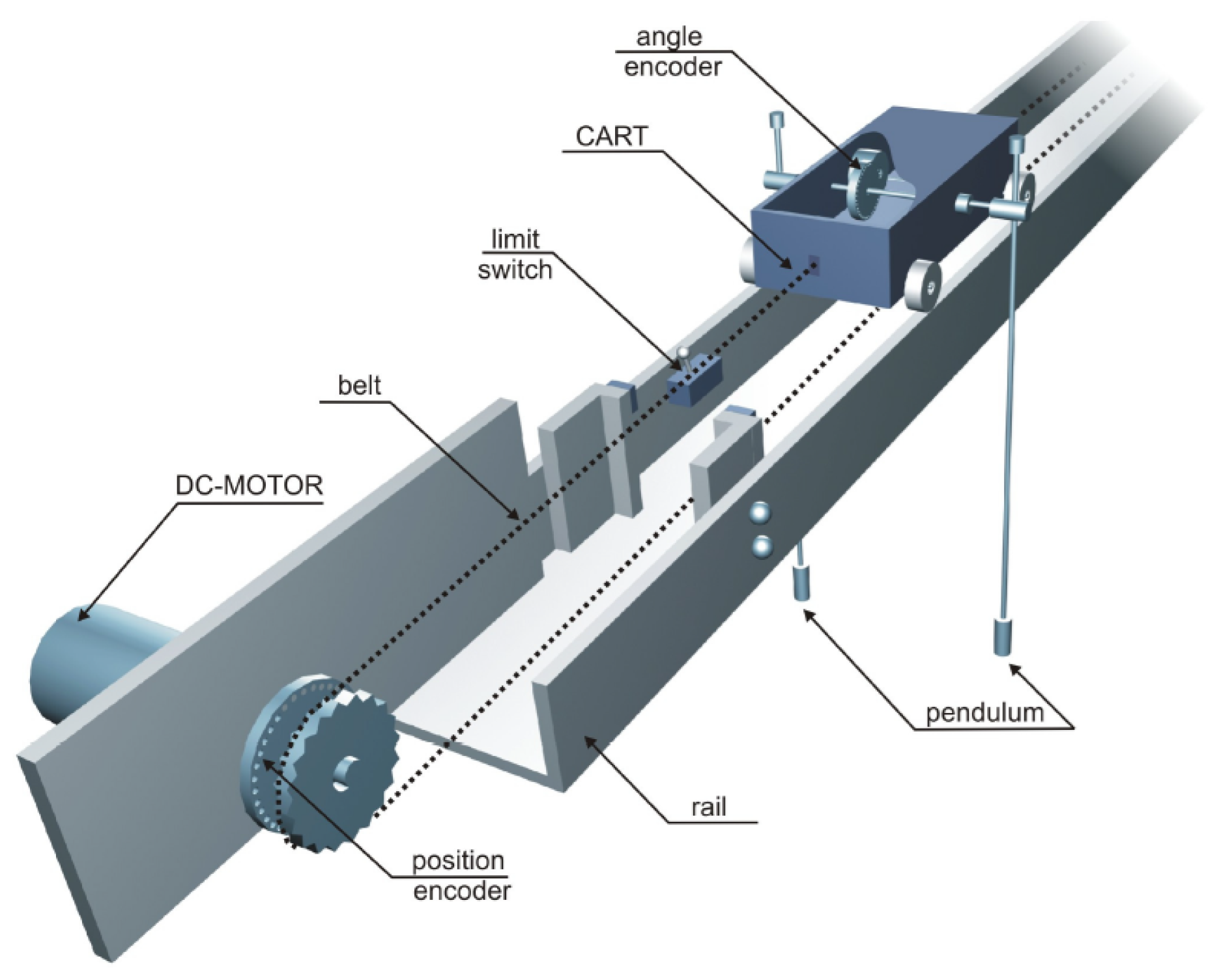
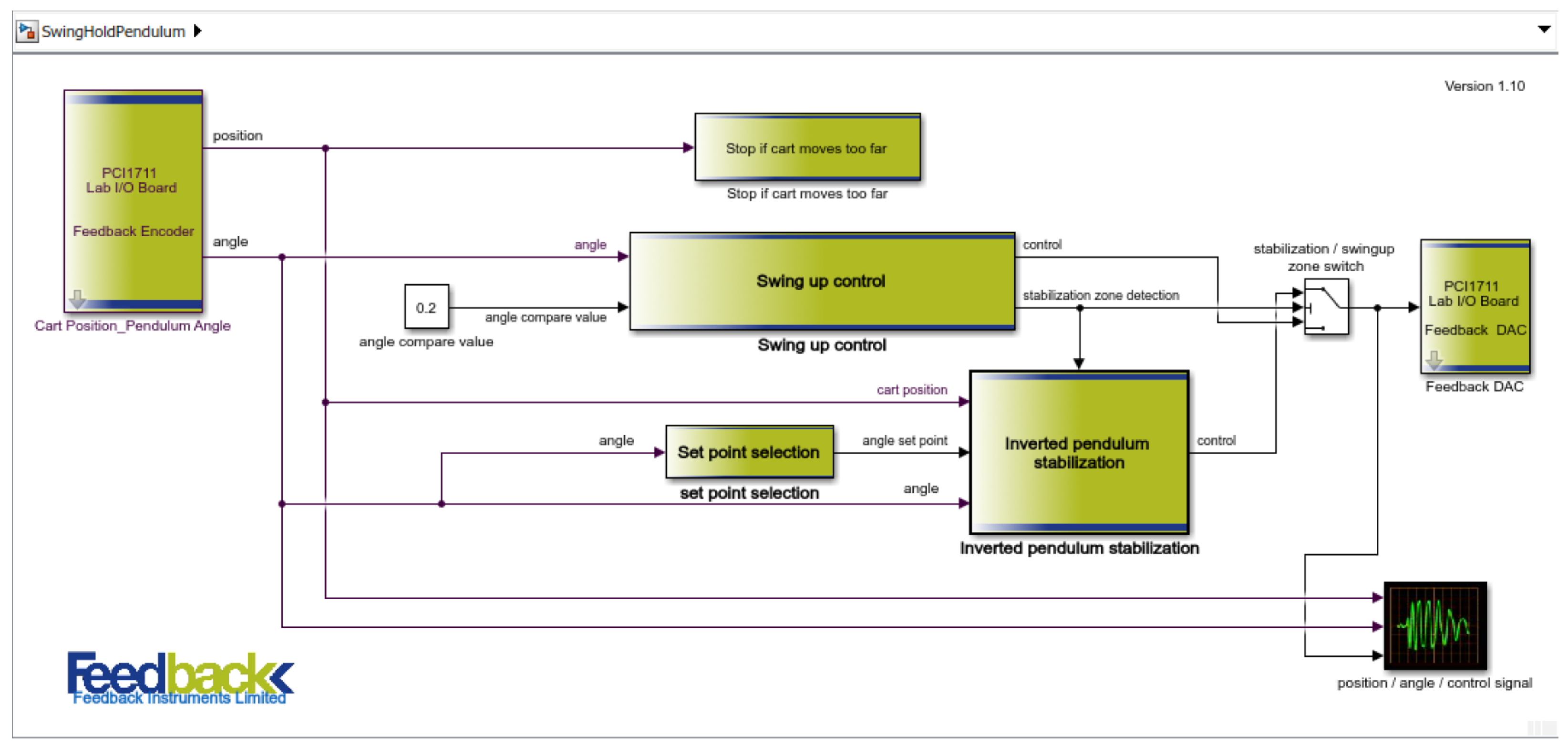
2.3. Inverted Pendulum System Description

The system to be controlled in this work corresponds to an Inverted Pendulum (InvP) system, manufactured by Feedback Instruments Ltd. Figure 1 shows a picture of the plant in the laboratory of the research group. A general diagram of this system, provided by the manufacturer, can be seen in Figure 2. The InvP system can be divided into three main components: the mechanical unit, the DC motor & interface unit, and the communication system.

The mechanical unit of the InvP includes all the mechanical elements of the system and essentially consists of a cart with two pendulums traveling on a rail [31]. The mechanical unit features a rail fixed to a base supported by two adjustable legs, which allows the rail to remain level. As illustrated in Figure 3, a direct current (DC) motor is positioned at one end of the rail, driving a sprocket wheel that, when in motion, moves a plastic toothed belt. This belt extends to the opposite end of the rail, where another sprocket wheel helps to maintain its tension before it returns to the motor’s end. A metal cart is connected to the plastic belt along the rail. A metal shaft in the center of the cart links two pendulums with mass at their longer ends, which can rotate freely. The movement of the cart is caused by the DC motor at the end of the rail, which pulls the belt in two directions. By applying voltage to the motor, the force with which the cart is pulled can be controlled. The force value depends on the control voltage applied to the motor, which rotates at a velocity proportional to the control voltage applied.

Both the cart shaft and the DC motor are equipped with optical encoders, enabling the measurement of the relative position of the cart and the relative position of the pendulum. An optical encoder comprises a light source, a light detector, and a slit disk positioned between them. This setup allows for the measurement of the relative position with respect to the initial point by counting the pulses detected by the light detector [31]. To obtain accurate data, the cart must be centered on the rail before any tests are conducted, and the pendulum should rest in the lower (hanging) position. These positions are defined as 0 [m] for the cart position and $\pi$ [rad] for the pendulum angular position, respectively. The cart can move freely along the rail, up to 1 [m] from the center in both directions. At these points, limit switches will activate if the cart reaches these positions, causing the DC motor to stop for safety reasons. In contrast, the pendulum can move through its full range from 0 [rad] to $2\pi$ [rad].

The DC motor and interface unit are responsible for receiving position signals from the optical sensors located in the mechanical unit and transmitting them to the computer, where the control algorithms will run. Similarly, it receives the control signal from the computer, which is a voltage ranging from −2.5 [V] to 2.5 [V], and sends it to the DC motor, which is also powered through this unit. Additionally, this unit executes the emergency stop if a limit switch is activated. It also features two buttons: a green button that allows tests to be conducted (enabling the inverted pendulum system to be used in experiments) and a red button that serves as a manual emergency stop.

The communication system comprises two fundamental components: a Small Computer System Interface (SCSI) adapter and a data acquisition card, specifically the Advantech PCI-1711U-CE. The SCSI adapter enables data and signal transmission between the computer and the mechanical unit, allowing real-time monitoring and control. The Advantech PCI-1711U-CE data acquisition card allows real-time data acquisition, which is essential for monitoring and controlling the system, and communicates with the computer through a Peripheral Component Interconnect (PCI) port. This card includes 16 analog input channels, two 12-bit analog output channels, 16 digital input channels, 16 digital output channels, a programmable counter, and a 12-bit analog/digital (A/D) converter with a sampling rate of up to 100 [kHz] [31]. Figure 4 illustrates the connection diagram between all the elements.

2.4. Mathematical Model of the Plant

To simulate the system as well as design, tune, and validate controllers for it, obtaining a sufficiently representative mathematical model of the system to be controlled is necessary. In the case of the InvP system, both the cart–pendulum and the DC motor must be modeled. In the case of the cart–pendulum system, the manufacturer provides a nonlinear model as follows [31]:

$$(M+m)\ddot{x}+b\dot{x}+ml\ddot{\theta }cos(\theta )-ml{\dot{\theta }}^{2}sin(\theta )=F,$$

(4)

$$(I+m{l}^2)\ddot{\theta }-mglsin(\theta )+ml\ddot{x}cos(\theta )+d\dot{\theta }=0,$$

(5)

where x [m] is the cart position with respect to the center of the rail, $\theta$ [rad] is the pendulum angular position with respect to the vertical, g is the gravitational acceleration, l is the pendulum length, M is the mass of the cart, m is the mass of the pendulum, I is the moment of inertia, b is the friction coefficient of the cart, d is the viscous friction coefficient of the pendulum, and F is the force applied to the cart by the motor and the input to the system. The numerical values of the eight specified parameters are listed in

Table 1. Numerical values of the model parameters for the InvP system (cart–pendulum and DC motor) [31].

Parameter	Value	Unit	Description
Cart–Pendulum System
g	9.81	[m/s2]	Gravitational acceleration
l	0.36	[m]	Pendulum length
M	2.4	[kg]	Mass of the cart
m	0.23	[kg]	Mass of the pendulum
I	0.099	[kg m2]	Moment of inertia
b	0.05	[N/rad/s]	Friction coefficient of the cart
d	0.005	[Nms/rad]	Viscous friction coefficient of the pendulum
DC Motor
Kt	0.05	[Nm/A]	Torque constant
Kb	0.05	[Vs/rad]	Electromotive constant
R	2.5	[Ω]	Electrical resistance
L	0.0025	[H]	Electrical inductance
J	0.000014	[Nms2/rad]	Rotor’s moment of inertia
B	0.000001	[Nms/rad]	Friction coefficient

. Although the manufacturer’s manual [31] provides only these nonlinear equations, they can be derived by defining the kinetic energy and potential energy, forming the Lagrangian, and obtaining the Lagrange equations for both the position of the cart (x) and the pendulum angular position ($\theta$). Details of this derivation are not included in this manuscript due to space constraints but can be found in [32].

Regarding the DC motor, it can be modeled as a resistor R in series with an inductance L, along with a voltage opposing the source (back electromotive force), which is generated by the motor’s angular velocity. Using Kirchhoff’s voltage law [33] and the rotational dynamics of the motor along with Newton’s second law, the following equations can be derived to describe the DC motor dynamics:

$$\begin{array}{ccc}\hfill J{\displaystyle \frac{dw(t)}{dt}}& =& K_{t}i(t)-Bw(t),\hfill \\ \hfill L{\displaystyle \frac{di(t)}{dt}}& =& v(t)-Ri(t)-K_{b}w(t),\hfill \end{array}$$

(6)

where i [A] is the current, v [V] is the source voltage, $\omega$ [rad/s] is the angular velocity, J is the inertial constant, B is the inertial moment with respect to the motor center of mass, $K_b$ is the electromotive constant, $K_t$ is the torque constant, R is the electrical resistance, and L is the electrical inductance. The numerical values of the six specified parameters can be found in Table 1. Since the DC motor model must be coupled with the cart–pendulum model, it is necessary to establish the mathematical relationship between the DC motor variables and the force F applied to the cart. In order to do this, the current–torque relationship and the torque–force relationship are used, both of which are included in the simulation software provided by the plant manufacturer [31] as follows:

$$T_m=K_{t}i,$$

(7)

$$F=600T_m,$$

(8)

where $T_m$ is the motor torque.

Once representative mathematical models of the cart–pendulum and DC motor are obtained, they are programmed in a computational environment. In this case, Matlab/Simulink R2022b is utilized, which is intuitive for modeling, simulating, and analyzing dynamic systems. Figure 5 illustrates a block diagram depicting the programmed structure. As shown in Figure 5, the input to the system corresponds to the voltage applied to the DC motor v, while the outputs are the pendulum’s angular position $\theta$ and the cart’s position x. In Matlab/Simulink, the DC motor Equations (6)–(8) are programmed into one block (DC motor block in Figure 5), whose input is the voltage applied to the motor, v, and the output is the force, F, applied to the cart. A second block (the one with the cart–pendulum in Figure 5) is then connected in series with the first block, which incorporates the nonlinear Equations (4) and (5). This second block takes the force F as input and produces the pendulum angular position, $\theta$, and the cart position, x, as outputs.

3. Controller Design and Tuning

The inverted pendulum control task can be seen as a self-erecting control problem, which is present in missile launching and control applications, to stabilize the inverted pendulum in an upright position. The inverted pendulum is inherently unstable. Left without a stabilizing controller, it will not be able to remain in an upright position when disturbed.

3.1. Controllers Included in the InvP System by the Manufacturer

The inverted pendulum control provided by the manufacturer is divided into two distinct control problems. The first is the swing-up control, which enables the pendulum to reach the upright position (around $\theta =0$) [rad]. The second involves controlling around that equilibrium point, which is achieved using PID control [31]. In the case of the swing-up control, the goal of the control is to bring the pendulum to an upright position with as minimal angular velocity as possible. This will ensure that the stabilizing controller, which takes over from the swing-up controller, will have an easy task. A large velocity value at the point of controller change could cause the pendulum to over swing; it could cause very volatile reactions of the cart or even cause it to hit the end of the track [31].

If the acceleration is unbounded, it is possible to bring the pendulum to the upright position in a single swing. However, for safety, it is better to swing up the pendulum in a robust way, which will ensure that the pendulum ends up in a vertical position where $\theta =0$. The motor control signal is bounded to ±2.5 [V] (the actual range is 0 [V] to +5 [V]) and ±20 [N] in terms of force, so these are the maximum values that can be transferred. The physical bound of the track also has to be considered [31]. There are many algorithms used for swing-up control; however, their robustness is in trade-off with their time performance. The manufacturer provides one strategy that achieves the control goal using a set of rules to define the control signal. Since the aim of this work is to propose controllers for the stabilization stage, the swing-up control provided by the manufacturer will be used without modifications.

For the stabilization stage, which is the main goal of this work, the manufacturer provides a PID controller. Since the inverted pendulum is a Single-Input Multiple-Output (SIMO) system, two separate PID controllers are provided (one for the angular position $\theta$ and one for cart position x), and their outputs are combined to generate the final single control signal, as can be observed in the block diagram of Figure 6. According to Figure 6 and the manufacturer manual, the control signal in the Laplace domain will be defined as

$$v(s)=\left[K_{p_{\theta }}+{\displaystyle \frac{K_{i_{\theta }}}{s}}+K_{d_{\theta }}s\right]e_{\theta }(s)-\left[K_{p_x}+{\displaystyle \frac{K_{i_x}}{s}}+K_{d_x}s\right]e_x(s),$$

(9)

where $K_{p_{\theta }}$, $K_{i_{\theta }}$, and $K_{d_{\theta }}$ are the proportional gain, integral gain, and derivative gain, respectively, of the PID controller for angular position. On the other hand, $K_{p_x}$, $K_{i_x}$, and $K_{d_x}$ denote the proportional gain, the integral gain, and the derivative gain, respectively, of the PID controller for the position of the cart. The control error for the position of the cart is expressed as $e_x=r_x-x$, while $e_{\theta }=r_{\theta }-\theta$ represents the error in the angular position of the pendulum, where $r_{\theta }$ and $r_x$ are the reference signals for the angular position of the pendulum and the position of the cart, respectively.

Since the goal is to center the cart on the rail and keep the pendulum in a stable upright vertical position, both the reference for the cart position $r_x$ and the reference for the pendulum’s angular position $r_{\theta }$ are set to zero. The manufacturer provided the numerical values of the controller gains as shown in

Table 2. Numerical values of the parameters for the PID_BASE controller provided by the manufacturer [31].

${\mathit{K}}_{{\mathit{p}}_{\mathit{x}}}$	${\mathit{K}}_{{\mathit{i}}_{\mathit{x}}}$	${\mathit{K}}_{{\mathit{d}}_{\mathit{x}}}$	${\mathit{K}}_{{\mathit{p}}_{\mathit{\theta }}}$	${\mathit{K}}_{{\mathit{i}}_{\mathit{\theta }}}$	${\mathit{K}}_{{\mathit{d}}_{\mathit{\theta }}}$
7	0.5	4	25	0.2	1.5

. These values were obtained using the Root Locus tool provided by the Matlab Control System Toolbox, together with a linearized model of the InvP. To do this, the manufacturer selected the desired location of the closed loop poles of the system, although no mention is made to the specific values used, just to the final gains obtained [31]. In the following sections, this controller will be referred to as PID_BASE.

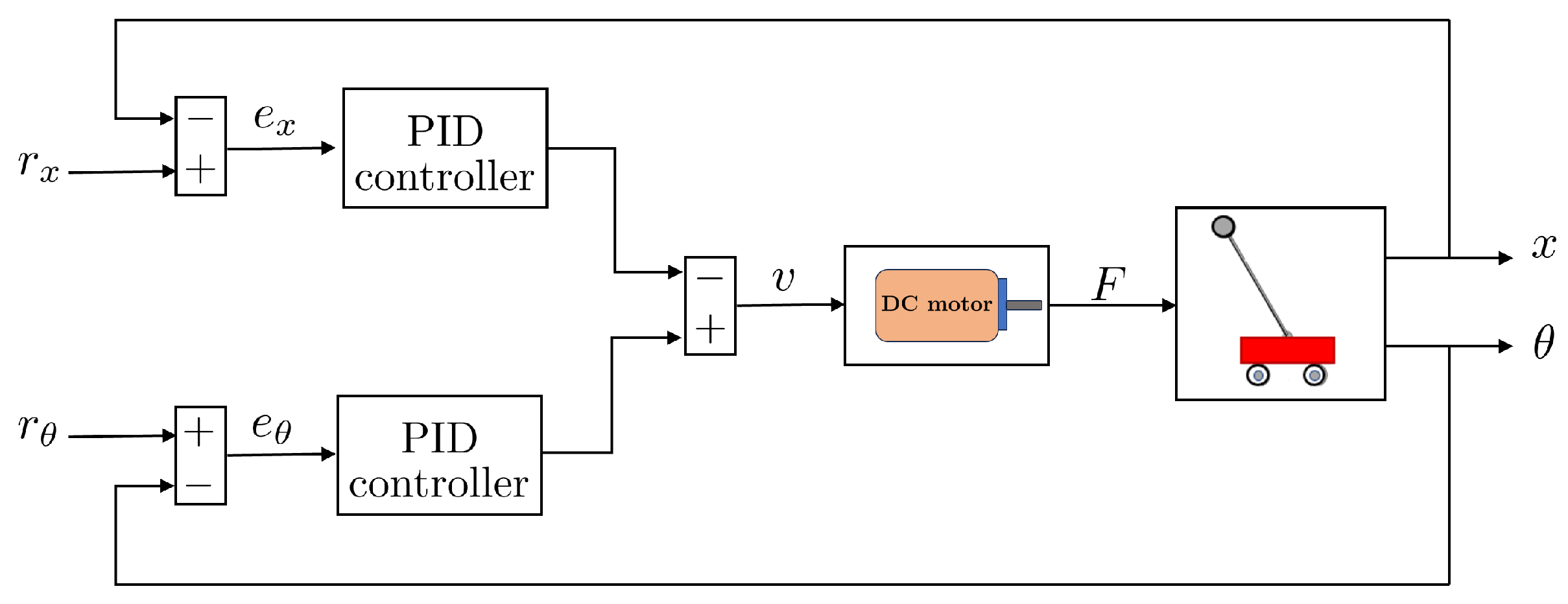
3.2. Design of the Switched Fractional-Order Proportional Integral Derivative Controller

A different tuning for PID controllers or the design and tuning of FOPID controllers could lead to improvements in control energy and system performance, compared to PID_BASE. However, these controllers can present a sort of trade-off between control energy and system performance, thus leading to the idea of using a switched version of them, trying to combine the strengths of both controllers. In the particular case of the inverted pendulum (PInv), the block diagram of the proposed strategy can be seen in Figure 7. A switching mechanism will allow one to alternate between a PID and FOPID controller, based on a criterion that, in this case, depends on the control error for the angular position $e_{\theta }$.

Specifically, the FOPID control signal will be sent to the plant when the absolute value of the angular position control error θ exceeds a certain threshold $e_s$ (design parameter), while the PID control signal will be sent when it is below this threshold. This means that the FOPID controllers would operate during transients and disturbed stages, providing their corresponding advantages, and the PID controllers would mostly operate near the steady state, offering their advantages of fast convergence. The equation representing the switched control scheme is therefore defined as follows:

$$v=\left\{\begin{array}{c}{u}_{FOPID}if|e_{\theta }(t)|>e_s\hfill \\ u_{PID}if|e_{\theta }(t)|\le e_s\hfill \end{array}\right.,$$

(10)

where $|e_{\theta }|$ corresponds to the absolute value of the control error of the pendulum’s angular position $e_{\theta }$, $e_s\ge 0$ is a design parameter, $u_{PID}$ is defined as in (9), and $u_{FOPID}$ is defined in the Laplace domain as

$$u_{FOPID}(s)=\left[K_{p_{{\theta }_f}}+{\displaystyle \frac{K_{i_{{\theta }_f}}}{s^{{\alpha }_{\theta }}}}+K_{d_{{\theta }_f}}{s}^{{\beta }_{\theta }}\right]e_{\theta }(s)-\left[K_{p_{x_f}}+{\displaystyle \frac{K_{i_{x_f}}}{s^{{\alpha }_x}}}+K_{d_{x_f}}{s}^{{\beta }_x}\right]e_x(s),$$

(11)

with $K_{p_{{\theta }_f}}$, $K_{i_{{\theta }_f}}$ and $K_{d_{{\theta }_f}}$ representing the proportional gain, integral gain and derivative gain, respectively, of the FOPID controller for the angular position. ${\alpha }_{\theta }$ and ${\beta }_{\theta }$ are the fractional orders for the integral part and the derivative part, respectively. On the other hand, $K_{p_{x_f}}$, $K_{i_{x_f}}$, and $K_{d_{x_f}}$ are the proportional gain, the integral gain, and the derivative gain, respectively, of the FOPID controller for the position of the cart, while ${\alpha }_x$ and ${\beta }_x$ are the fractional orders of the integral and derivative parts of this controller, respectively.

To implement the switched control scheme, we decided to filter the control signal v (as shown in Figure 7) to smooth it before injecting it into the system. This is necessary because switching between control schemes can lead to abrupt transitions, which should be avoided for the protection of actuators. The filter used is a first-order transfer function defined by

$$H(s)={\displaystyle \frac{1}{{\tau }_{f}s+1}},$$

(12)

where s represents the complex variable in the Laplace domain, and ${\tau }_f$ is the time constant. As shown in (12), incorporating this filter into the control scheme adds a pole to the system, which remains stable for any positive value of ${\tau }_f$. The time constant ${\tau }_f$ adjusts the speed of the filter response. A smaller value of ${\tau }_f$ enables the filter to pass higher frequency signals, resulting in a faster response but with a less smoothing effect on transitions. On the other hand, a larger value of ${\tau }_f$ will provide a greater smoothing effect but may introduce a delay in the system’s response. Therefore, there is a trade-off between smoothing and delay, so the process of selecting the time constant ${\tau }_f$ must be carried out carefully. For simulation purposes and controller tuning, a value of ${\tau }_f=0.001$ was established and maintained in the experimental tests. The tuning process was conducted through trial and error.

3.3. Tuning of Controller Parameters

According to the structure of the switched controller proposed in Section 3.2, the number of parameters to be tuned using the optimization process is 17, of which 6 correspond to the PID controllers, 10 correspond to the FOPID controllers, and the last corresponds to the threshold value $e_s$, which is compared to the absolute value of the error to determine when to switch. The parameter vector to be adjusted is therefore defined as follows.

$$\begin{array}{cc}\hfill p=[& \stackrel{\mathrm{PID}}{\overbrace{K_{px}{K}_{ix}{K}_{dx}{K}_{p\theta }{K}_{i\theta }{K}_{d\theta }}}\stackrel{\mathrm{FOPID}}{\overbrace{K_{p{x}_f}{K}_{i{x}_f}{K}_{d{x}_f}{\alpha }_x{\beta }_x{K}_{p{\theta }_f}{K}_{i{\theta }_f}{K}_{d{\theta }_f}{\alpha }_{\theta }{\beta }_{\theta }}}{e}_s],\hfill \end{array}$$

(13)

where the subscript f in the gains refers to the FOPID controller. Due to the large number of controller parameters to be tuned, an offline optimization process was conducted, specifically using particle swarm optimization (PSO) and using the mathematical model of the system for simulation purposes.

Before starting the controller tuning process with an optimization algorithm, it is essential to establish the criteria that the algorithm will use to evaluate and refine the design parameters. To achieve this, the system’s performance is assessed according to two criteria: the performance of the controlled system and the use of control energy. These performance indices will also facilitate conclusions about the impact of the design parameters and the pros and cons of the resulting controllers during a later comparison of results. The performance of the controlled system is evaluated through the integral of the time-weighted absolute error (ITAE), which is given by

$$ITAE=\underset{0}{\overset{T_i}{\int }}t|e(t)|dt,$$

(14)

where $T_i$ corresponds to the simulation/operation time of the controlled system at the time of controller tuning, and e to the control error of the system, in this case considering both the error in angular position and the error in the cart position, i.e., $e=e_x+e_{\theta }=(r_x-x)+(r_{\theta }-\theta )$. In the case of control energy, it is evaluated through the integral of the squared control signal ($ISI$), in this case

$$ISI=\underset{0}{\overset{T_i}{\int }}{v}^2\left(t\right)dt,$$

(15)

where v corresponds to the control signal injected into the system. This index allows us to measure the effort required to control the system, which translates into control energy. In that way, the cost function to be optimized during the tuning corresponds to the combination of both performance indexes, that is

$$J=ITAE+ISI.$$

(16)

The search space must be defined by setting the range of values that the parameters of p (13) can take, establishing an upper bound $(ub)$ and a lower bound $(lb)$. The search range for gains was set to ±50, while the range for the values of integral and derivative orders was defined as (0, 1.9), since this range ensures a necessary (though not sufficient) condition for the stability of a fractional-order system [30]. Since the controllers are designed to operate within the range of ±0.2 [rad] because they will address only the stabilization (not the swing-up), and considering that the absolute value of the error serves as the switching element, for the $e_s$ parameter, the lower and upper limits were set to 0 and 0.2 [rad], respectively.

For optimization, Matlab’s PSO toolbox was used. The number of particles, $noP$, was set to 200, the maximum number of iterations to $maxIter=200$, and the remaining algorithm parameters were maintained at their default values. Furthermore, the code was modified to start the search from the gains of the PID_BASE controller, for both the PID and the FOPID, with fractional orders equal to 1 for the latter and $e_s=0.2$, allowing the search to start from a stable and feasible controller. To carry out the optimization process, each parameter vector p (13) was used to run the pendulum stabilization simulation. Each simulation begins with the cart positioned at 0 [m] and the pendulum tilted at 0.2 [rad], which is roughly 11 degrees. The simulation duration for all experiments was established at 100 [s]. Upon concluding each simulation, the ITAE and ISI were calculated, and the cost function was computed, which was then sent back to the PSO algorithm to proceed with the search.

The parameter values resulting from the optimization process are shown in

Table 3. Resulting parameters from the optimization process for all designed controllers.

	${\mathit{K}}_{\mathit{p}}$	${\mathit{K}}_{\mathit{i}}$	${\mathit{K}}_{\mathit{d}}$	$\mathit{\alpha }$	$\mathit{\beta }$	${\mathit{e}}_{\mathit{s}}$
SW-FOPID-PID controller
${\mathrm{PID}}_x$	8.85	0.86	6.82	-	-	0.12
${\mathrm{PID}}_{\theta }$	19.11	5.25	3.61	-	-
${\mathrm{FOPID}}_x$	−2.25	2.43	0.88	0.91	0.40
${\mathrm{FOPID}}_{\theta }$	33.41	0.78	−2.17	1.56	0.56
PID controller
${\mathrm{PID}}_x$	4.53	0.58	4.82	-	-	-
${\mathrm{PID}}_{\theta }$	8.95	1.61	2.44	-	-	-
FOPID controller
${\mathrm{FOPID}}_x$	2.02	3.32	11.13	0.86	0.56	-
${\mathrm{FOPID}}_{\theta }$	48.36	−0.03	6.27	1.08	0.69	-

. Additionally, Table 3 includes non-switched PID and FOPID controllers, which were designed and tuned using the same procedure as the switched controller for comparison purposes. As can be observed, for the PID controller, the gain values obtained are all positive and relatively small in magnitude. In contrast, for the switched SW FOPID-PID controller, the parameter $e_s$ resulted in 0.12 [rad] (approximately 6.87 degrees), which is around the midpoint of the operating region for the stabilization controller. For FOPID controllers, the optimization algorithm produced controllers that lacked the derivative component $K_d$ (the order $\beta$ took a value of zero), which means that they were actually FOPI controllers. However, these controllers faced difficulties during experimental validation; they could achieve stabilization but at the cost of a control signal that caused the cart to move very quickly, leading to the suspension of the experiment for safety reasons regarding the plant’s components.

Consequently, we decided to repeat the tuning process for this controller, adding constraints to the algorithm’s search ranges in an attempt to reverse the previous outcomes. The ranges for controller gains were restricted to low positive values, and the range for fractional orders was limited to [0.2, 1.5] to prevent very slow control signals (orders less than 0.2) or highly oscillatory control signals (orders greater than 1.5). As a result, a new set of parameters was obtained for the FOPID controller, showing significant improvement in the behavior of this controller during stabilization. This set of parameters is shown in Table 3.

4. Experimental Validation of Controllers

To perform real-time tests of the proposed controllers, two elements must be considered that were not present during the simulation environment used for tuning. The first is how data might be obtained from the plant’s sensors in Matlab/Simulink, and the second is how the control signal generated by the controllers may be sents from Matlab/Simulink to the plant. Specific tools for these tasks in Matlab/Simulink are included in the software provided by the plant manufacturer [31]. The Feedback Encoder block, whose image is shown in Figure 8, is responsible for extracting information from the Advantech PCI-1711U-CE card, which establishes communication between the computer and the plant. This block provides the data for the cart position x [m] and the angular position of the pendulum $\theta$ [rad], with a sampling frequency of 1 [kHz].

The second block provided by the manufacturer’s software [31] is the Feedback DAC, which converts the control signal of the system into a voltage signal compatible with the physical system. Figure 9 shows an image of this block. To ensure proper operation of the plant, the software provided by the manufacturer for Matlab/Simulink also includes three safety components. The first is a Friction compensator, which helps to compensate for the effects of friction in the cart–pendulum system and improve control accuracy. The second corresponds to a Saturator, which limits the control voltage sent to the plant to a maximum range of ±2.5 [V]. Finally, the third is a Voltage scaler, used to add 2.5 [V] to the control signal to adjust the voltage ranges to those utilized by the Advantech PCI-1711U-CE communication card, as it has a unipolar DAC output ranging from 0 to 5 [V].

To bring the pendulum to the stabilization region where the proposed controllers will operate, the swing-up algorithm included in the plant software [31] was used. To integrate the proposed controllers with this swing-up stage, the block called Swing hold pendulum extra included in the software was utilized, as shown in the block diagram in Figure 10. As can be observed in Figure 10, this diagram incorporates a block responsible for lifting the pendulum and the other elements needed for its subsequent control in the stabilization zone. Therefore, the control block Inverted pendulum stabilization was replaced with the controllers designed in this work, while the lifting block Swing-up control remained as it appeared in the experiment.

The block responsible for lifting starts to operate with the pendulum in the position π [rad], equivalent to its stable lower position (free hanging). To initiate the pendulum’s swing, the cart is moved in one direction until the derivative of the pendulum’s angular position reaches zero, after which the cart’s movement is reversed. With each repetition of this process, the pendulum reaches a greater height. When the pendulum exceeds the horizontal position of $\pm {\displaystyle \frac{\pi }{2}}$ [rad], the cart reverses its direction, aiding the pendulum in rising even higher until it reaches a position of ±0.2 [rad]. At this point, the system switches from the lifting block to the control block (stabilizing control). It is crucial to note that the lifting block incorporates a PID controller that stabilizes the cart’s oscillations around the origin, preventing it from moving to the ends of the rail, where limit switches would stop the experimental test if activated.

Additionally, this experiment includes the block Set point selection. As shown in Figure 10, this block addresses an issue that was not considered at the simulation level when the controllers were tuned, where the stabilization reference was always set at 0 [rad], but the pendulum can also stabilize at the position $2\pi$ [rad]. This block changes the stabilization reference depending on which side the pendulum is moving. If the pendulum reaches values greater than $\pi$ [rad], it will stabilize at $2\pi$ [rad]; otherwise, if the values are less than $\pi$ [rad], it will use 0 [rad] as the reference.

4.1. Results and Discussion of Experimental Validation

The experimental tests were carried out for all proposed controllers, as well as for the PID_BASE included with the manufacturer’s software, for comparison purposes. The performance of the controllers is analyzed only for the stabilization phase of the pendulum, taking as the initial time the moment in which the transition from the lifting phase (common to all controllers) to the stabilization phase occurs. For the comparative analysis of each control scheme, the ISI and ITAE performance indicators are used. Note that these performance indicators are integrals calculated over the whole experiment and thus represent the overall control energy used and error performance, respectively. The peak values ($Peak$) and settling times ($T_s$) are also used as performance indicators, both for the cart position x and the angular position $\theta$. In the case of settling times, a tolerance of $5\%$ of the corresponding variable range is used to calculate their values. Additionally, the variance ($\sigma$) of controlled and manipulated variables is incorporated to assess the impact of the natural oscillations that occur in real experiments due to measurement noise, etc.

The resulting performance indicators are shown in

Table 4. Results obtained for the performance indicators in experimental tests to stabilize the InvP system using the designed controllers.

	$\mathit{ISI}$	$\mathit{ITAE}$	${\mathit{Peak}}_{\mathit{x}}$	${\mathit{Peak}}_{\mathit{\theta }}$	${\mathit{T}}_{{\mathit{s}}_{\mathit{x}}}$	${\mathit{T}}_{{\mathit{s}}_{\mathit{\theta }}}$	${\mathit{\sigma }}_{\mathit{v}}$	${\mathit{\sigma }}_{\mathit{x}}$	${\mathit{\sigma }}_{\mathit{\theta }}$
PIDBASE	4.75	7.34	0.18	0.19	5.99	17	2.79 $\times {10}^{-1}$	1.90 $\times {10}^{-3}$	1.10 $\times {10}^{-3}$
SW FOPID-PID	2.91	0.20	0.07	0.015	0.45	0.94	1.71 $\times {10}^{-1}$	1.71 $\times {10}^{-4}$	1.09 $\times {10}^{-4}$
FOPID	3.66	3.85	0.13	0.13	4.38	17	2.15 $\times {10}^{-1}$	1.50 $\times {10}^{-3}$	3.35 $\times {10}^{-4}$
PID	1.46	6.57	0.09	0.05	4.35	16.8	8.53 $\times {10}^{-2}$	7.26 $\times {10}^{-4}$	1.82 $\times {10}^{-4}$

. For visual reference, Figure 11 shows the cart position x, the angular position of the pendulum $\theta$, and the control signal v. Note that although the stabilization phase lasted 17 [sec], the x-axis shows only the transient for better visualization. On the other hand, Figure 12 and Figure 13 show how ITAE and ISI evolve over time. Based on the results, the following conclusions can be drawn.

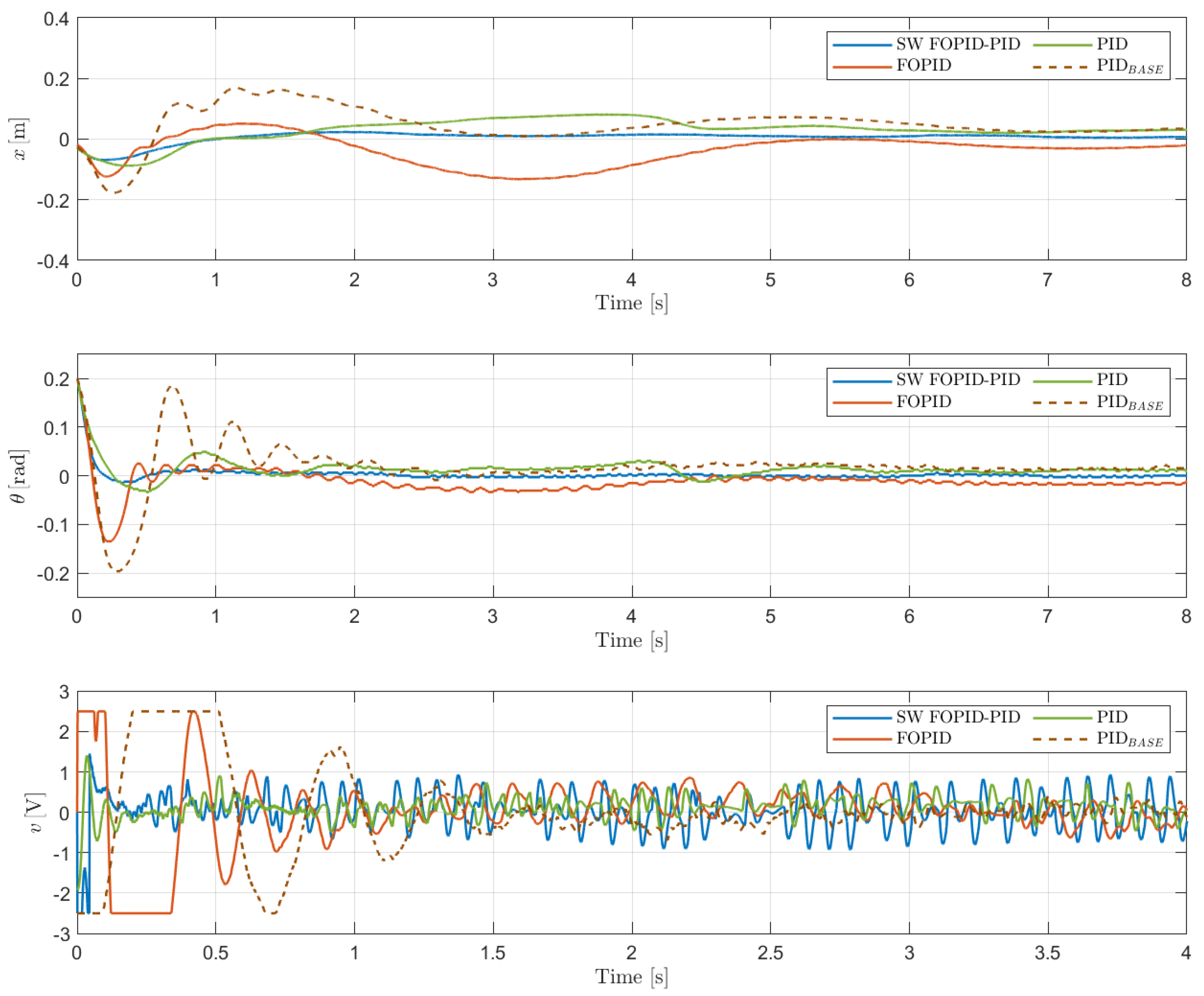
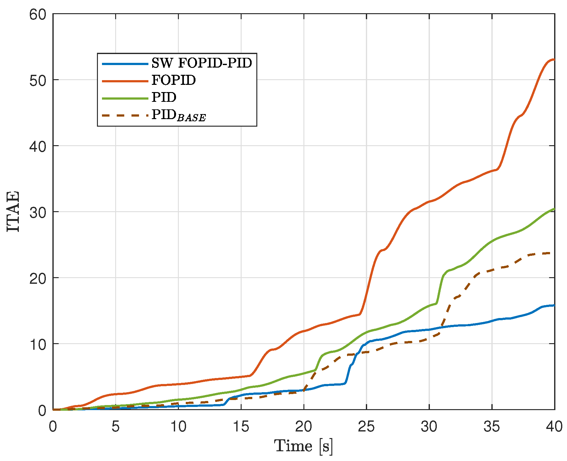
• The SW FOPI-PID controller has the lowest ITAE, with a significant margin compared to the other controllers. This is illustrated in Figure 11, which shows that this controller stabilizes both states fairly quickly. Additionally, Figure 12 shows that ITAE converges rapidly and reaches a much lower value compared to the rest of the controllers.
• In addition to having the lowest ITAE value, the SW FOPID-PID controller presents the lowest peak values and settling times for both the cart position and the pendulum angular position. Furthermore, this controller produced the lowest variances in both the pendulum angular position and cart position. Together with the previously mentioned results, this indicates that the switched controller performs the best.
• The only downside of this controller, as shown in Figure 11, is that its control signal saturates briefly at the beginning of the experiment and exhibits oscillations throughout the entire control process, leading to an increase in the ISI indicator. Nevertheless, the control energy used in this case lies in between the values obtained with the proposed PID and FOPID controllers, as can be corroborated from Figure 13 and Table 4. Note that this brief saturation does not have any significant effect in the controlled variables of the inverted pendulum, as can be observed from Figure 11, where both the cart position x and the pendulum angular position $\theta$ have smooth behaviors during that initial time and throughout the whole experiment. Moreover, the PID_BASE and the FOPID also saturate for time periods even longer than the switched controller, with the PID_BASE controller being the one that saturates for the longest time. Only the PID tuned in this work does not present saturation at the beginning of the simulation, but again, the switched controller exhibits better performance indicators for the controlled variables, which makes its brief saturation something that can be tolerated, since it does not represent risks for system actuators. Also, the switched controller outperforms the PID_BASE controller provided by the manufacturer and the designed FOPID controller in every single performance metric shown in Table 4. To summarize, it can be concluded that the switched controller not only achieves the best performance but also does so with a balanced use of control energy, compared to the non-switched controllers.
• The proposed PID controller exhibits the lowest ISI due to a smoother control signal with smaller oscillations, as shown in Figure 11. However, this leads to longer rise times compared to the FOPID and SW FOPID-PID controllers. Nevertheless, the proposed PID outperforms the manufacturer’s PID_BASE controller in every single indicator.
• The FOPID controller, as previously mentioned, presented several difficulties during the experimental tests, generating very abrupt responses, and despite managing to control the pendulum, the test had to be suspended due to very rapid oscillations of the cart. This was largely mitigated by retuning the controller, allowing for complete tests to be carried out without major issues, but as seen in Figure 11, the described tendency remains when observing the control signal of the controller. It saturated on more than one occasion and exhibited a greater number of oscillations with larger magnitudes, a behavior that can also be seen in the angular position of the pendulum, which showed small ripples throughout the experiment. Still, looking at the performance indicator data in Table 4, this controller outperforms the proposed PID in ITAE and has pretty similar values for settling times; it outperforms the manufacturer PID_BASE controller in every indicator.
• Finally, we refer to the analysis of the variances of the signals during the control process, which were added to visualize the magnitude of the parameter and provide valuable information about the stability and accuracy of the controlled system. Table 4 shows the values obtained for this indicator for the cart position, pendulum angular position, and control signal for each of the controllers under study. The PID controller has the lowest variance for the control signal, followed by the switched SW FOPID-PID controller. This result is consistent with what is observed in Figure 11, where the control signals of these two controllers show the smallest magnitudes in their oscillations. In contrast, controllers like FOPID and PID_BASE show an increase in this indicator compared to the others, making more frequent and larger adjustments, a situation that could cause wear on the system’s actuators.
• For both the cart position and the pendulum’s angular position, the variances for the PID and SW FOPID-PID controllers are quite similar, with the latter exhibiting the lowest values. This indicates that both controllers maintain both state positions with little deviation, resulting in good control performance. The FOPID and PID_BASE controllers, on the other hand, exhibit higher magnitudes for these variances, with lower values for the FOPID in the pendulum angular position and fairly similar values for the cart position in both. This means they show greater fluctuations in the positions and that the control exerted is effective but inferior in terms of performance compared to the switched SW FOPID-PID and PID controllers. The lower values of these indicators for these latter controllers may indicate that the controlled system is more robust against disturbances.

4.2. Results and Discussion of Experimental Validation in the Presence of Disturbances

Once the experiments mentioned in the previous section were concluded, the robustness of the controllers was tested in the presence of disturbances. To do this, the experiments were conducted similarly to the previous case, but after completing the pendulum’s lifting phase and stabilization, it was manually pushed at the end at which the mass is located. This introduced a disturbance in the angular position, which was also reflected in the cart position. This push was applied more than once during the experiments. The test carried out may not be entirely conclusive in determining how certain controllers outperform others, as experiments were, of course, carried out separately for each controller, meaning that the force applied manually to the pendulum as a disturbance was not of the same magnitude in all cases.

However, it does help to verify the robustness of the designed controllers. Only for reference, the resulting deviations of the controlled variables after the disturbances are applied are specified in the following, using degrees and centimeters for better intuitiveness. When using the SW FOPID-PID controller, the first disturbance was applied around $t=13.5$ [s] and the second was applied around $t=23.5$ [s], resulting in deviations of ($\theta =5.08$ degrees, $x=8.6$ [cm]) and ($\theta =10.7$ degrees, $x=14.9$ [cm]), respectively. For the PID controller, the first disturbance was applied around $t=20.8$ [s], and the second was applied around $t=30.5$ [s], resulting in deviations of ($\theta =6.85$ degrees, $x=11.8$ [cm]) and ($\theta =8.43$ degrees, $x=15.3$ [cm]), respectively. The FOPID controller received strikes around $t=15.7$ [s] and $t=24.4$ [s], resulting in deviations of ($\theta =3.16$ degrees, $x=14.5$ [cm]) and ($\theta =4.41$ degrees, $x=24.1$ [cm]), respectively. Finally, the PID_BASE controller was perturbed around $t=19.8$ [s] and $t=30.7$ [s], resulting in deviations of ($\theta =5.45$ degrees, $x=11.3$ [cm]) and ($\theta =6.15$ degrees, $x=12.9$ [cm]), respectively.

As in the experiments without disturbances, only the stabilization phase was considered when calculating the performance indicators, without taking into account the time it took the system to complete the lifting phase. The results obtained for the performance indicators in these tests are shown in

Table 5. Results obtained for the performance indicators in experimental tests to stabilize the InvP system using the designed controllers, in the presence of disturbances.

	$\mathit{ISI}$	$\mathit{ITAE}$	${\mathit{Peak}}_{\mathit{x}}$	${\mathit{Peak}}_{\mathit{\theta }}$	${\mathit{T}}_{{\mathit{s}}_{\mathit{x}}}$	${\mathit{T}}_{{\mathit{s}}_{\mathit{\theta }}}$	${\mathit{\sigma }}_{\mathit{v}}$	${\mathit{\sigma }}_{\mathit{x}}$	${\mathit{\sigma }}_{\mathit{\theta }}$
PIDBASE	5.24	23.85	0.13	0.14	33.58	36.86	0.13	1.1$\times {10}^{-3}$	3.3 $\times {10}^{-4}$
SW FOPID-PID	5.09	15.81	0.14	0.18	24.64	25.62	0.12	4.16 $\times {10}^{-4}$	5.8 $\times {10}^{-4}$
FOPID	8.82	53.05	0.36	0.15	39.31	39.46	0.22	9.0 $\times {10}^{-3}$	6.9 $\times {10}^{-4}$
PID	4.54	30.43	0.15	0.16	33.76	40	0.11	1.0 $\times {10}^{-3}$	3.4 $\times {10}^{-4}$

. Figure 14 shows the evolution of the controlled and manipulated variables, while Figure 15 and Figure 16 show the evolution of ITAE and ISI, respectively. Based on these results, the following conclusions and remarks can be made.

• Similar to cases without disturbances, the switched controller resulted in the lowest ITAE and settling times for both the cart position and the pendulum’s angular position. It also yielded the lowest value for the variance of x. Although the lowest peak values and the variance of $\theta$ were achieved with the manufacturer PID_BASE, this does not mean the PID was actually better in these performance indices, due to the points discussed in the following section.
• Although the PID_BASE controller provided by the manufacturer showed the lowest peak values and variance for $\theta$, outperforming SW FOPID-PID, and many of the remaining performance indicators were better than with PID and FOPID controllers, this result is not completely representative and cannot allow full conclusions to be drawn. This is because in the case of PID_BASE, several tests were needed to finish this experiment successfully. In most experiments, applying a second strike caused the pendulum to fall, or the cart, while trying to control it, would move to the end of the rail, triggering a limit switch and stopping the simulation. It can be seen from Figure 14 that disturbances applied to this controller were of lower magnitude, as that was the only way for the controller to recover after two strikes. Thus, it was obvious that the peak values and variance of $\theta$ would be lower for this controller. It is important to note that although in this test the depicted PID_BASE used a lot of control energy in attempting to stabilize the pendulum after the strikes, once the pendulum was stable, it required less energy compared to the other controllers. This can be seen in the ISI plot in Figure 16, where the slope after the disturbances is the lowest.
• Although the strikes applied to the PID tuned in this work were of higher magnitude than those for the PID_BASE, it also encountered issues in successfully completing the experiments. Several attempts were necessary in order to achieve a test in which the PID was able to stabilize completely after two strikes, due to the same reasons explained in the previous point for PID_BASE. Still, as can be seen from Table 5 and Figure 16, the PID is the controller with the lowest ISI, as in the case without disturbances. However, the differences with respect to the ISI for the rest of the controllers are not as representative as in the previous experiments.
• The FOPID controller demonstrated greater robustness than the previous two controllers. This was confirmed by its ability to apply multiple disturbances to the system without the pendulum falling or the cart deviating too much (three strikes can be seen in Figure 14 for this controller). However, it was necessary to include a speed filter in the generated control signal, as the system oscillated faster than the actuator could handle in the steady state, which could have caused problems with the setup. This filter helped in improving the steady state, achieving a low slope in both ITAE (see Figure 15) and ISI (see Figure 16). Nevertheless, the filter also negatively affected the controller’s performance in the transient states, as reflected in the slopes of ISI and ITAE at those moments and leading to this controller being the one with the highest values for both ITAE and ISI.
• Although the switched SW FOPID-PID controller was not the best in terms of energy performance, as seen in Figure 16, which shows a steeper slope in the steady state, the resulting value for ISI was in between the values used for PID and FOPID controllers, as it was in the case without disturbances. Considering all the previous analyses, it can be concluded that the SW FOPID-PID controller resulted in the best overall performance. Moreover, it was evident during the tests that it was the most robust controller, as it withstood stronger strikes and managed to remain stable in all cases.

4.3. Limitations and Future Work

As part of this work, we attempted to design and experimentally validate two more controllers for comparison purposes. The first was a Linear Quadratic Regulator (LQR) controller, which is one of the most common control strategies used for the InvP. In this work, an LQR controller was designed, tuned, and successfully tested at the simulation level. However, it was not possible to test it experimentally because, being a state-space controller, it needed all the state variables for practical implementation. That means that it needed not only the cart position x and pendulum angular position $\theta$, but also the cart speed $\dot{x}$ and angular speed of the pendulum $\dot{\theta }$. This imposed a practical restriction, since the plant does not have sensors to measure speeds, and thus it was not possible to implement the LQR controller. An alternative discussed to overcome this issue was including a state observer for these two variables, which is something currently being investigated.

The other kind of controller that we attempted to design this work was a Model Reference Adaptive Controller (MRAC). However, the tuning of this controller was not successful, as the optimization procedure did not find a set of controller parameters that could effectively stabilize the pendulum; this is why it was also not included in the study. However, different optimization techniques are currently being used in order to obtain an effective MRAC for the InvP system. Changes in the structure of the MRAC controller were also taken into account.

In addition, as a future work, alternative switching criteria for the controllers will be investigated. Since this work mainly focused on minimizing the angular error of the pendulum, that was the error used in the switching criterion. However, the cart position was also being controlled, and thus it made sense to use a different switching criterion for them (for instance, using $e_x$ rather than $e_{\theta }$).

Finally, we would like to mention that while the conclusions drawn from this study are supported by the experimental results on the InvP system, it is important to recognize that an inverted pendulum is a specific benchmark system with its own unique characteristics. Therefore, generalizing the conclusions, and by that we mean the usefulness of the SW FOPID-PID controller to broader classes of control systems, would require additional experimental studies on different plants.

5. Conclusions

In this paper, PID, FOPID, and switched SW FOPID-PID controllers were designed, implemented, and tuned to stabilize an inverted pendulum system (InvP). The tuning of the controllers was performed offline using particle swarm optimization and a mathematical model of the system for simulation purposes. The experimental validation of the controllers was carried out with and without external disturbances. Performance indicators such as ITAE, ISI, and controlled variables’ settling times, peak values, and variances were used to analyze the controlled system performance. A PID controller provided by the InvP system manufacturer was used for comparison.

In the case without disturbances, the three designed and tuned controllers outperformed the manufacturer’s PID across every performance indicator. The switched SW FOPID-PID controller achieved the lowest values for all performance indicators, except control energy and control signal variance, where the designed PID performed the best. However, the control energy used by the SW FOPID-PID yielded values between those obtained with the PID and the FOPID, achieving the desired balance. When a manual disturbance was applied to the InvP, the FOPID and SW FOPID-PID controllers were more robust than the designed PID and manufacturer’s PID, as they could withstand multiple disturbances without the pendulum falling or the cart deviating excessively. However, the FOPID required a speed filter, which impacted other performance indicators. Thus, the switched controller emerged as the most robust, able to withstand large impacts and respond quickly; it generated minimal errors in both the cart’s and the pendulum’s angular positions.

Future work will explore alternative switching criteria for the controllers, as in this work we primarily focused on minimizing the angular error of the pendulum, which was the error used in the switching criterion. In addition, the design and experimental validation of LQR controllers with state observers and adaptive controllers will be investigated.

References

1. Tepljakov, A.; Alagoz, B.B.; Yeroglu, C.; Gonzalez, E.A.; Hosseinnia, S.H.; Petlenkov, E.; Ates, A.; Cech, M. Towards Industrialization of FOPID Controllers: A Survey on Milestones of Fractional-Order Control and Pathways for Future Developments. IEEE Access 2021, 9, 21016–21042. [Google Scholar] [CrossRef]
2. Pataro, I.M.L.; Gil, J.D.; Alvarez, J.D.; Guzmán, J.L.; Berenguel, M. Robust Fractional Order PID Controller Coupled with a Nonlinear Filtered Smith Predictor for Solar Collector Fields. IFAC-PapersOnLine 2025, 58, 234–239. [Google Scholar] [CrossRef]
3. Ghamari, S.M.; Molaee, H.; Ghahramani, M.; Habibi, D.; Aziz, A. Design of an Improved Robust Fractional-Order PID Controller for Buck–Boost Converter using Snake Optimization Algorithm. IET Control Theory Appl. 2025, 19, e70008. [Google Scholar] [CrossRef]
4. Basil, N.; Mohammed, A.F.; Sabbar, B.M.; Marhoon, H.M.; Dessalegn, A.A.; Alsharef, M.; Ali, E.; Ghoneim, S.S.M. Performance analysis of hybrid optimization approach for UAV path planning control using FOPID-TID controller and HAOAROA algorithm. Sci. Rep. 2025, 15, 4840. [Google Scholar] [CrossRef]
5. Paliwal, S. Stabilization of Mobile Inverted Pendulum Using Fractional Order PID Controllers. In Proceedings of the 2017 International Conference on Innovations in Control, Communication and Information Systems (ICICCI), Greater Noida, India, 12–13 August 2017; pp. 1–4. [Google Scholar] [CrossRef]
6. Asadollahi, M.; Rikhtegar ghiasi, A.; Dehghani, H. Excitation control of a synchronous generator using a novel fractional-order controller. IET Gener. Transm. Dis. 2015, 9, 2255–2260. [Google Scholar] [CrossRef]
7. Oróstica, R.; Duarte-Mermoud, M.A.; Jáuregui, C. Stabilization of inverted pendulum using LQR, PID and fractional order PID controllers: A simulated study. In Proceedings of the 2016 IEEE International Conference on Automatica (ICA-ACCA), Curico, Chile, 19–21 October 2016; pp. 1–7. [Google Scholar] [CrossRef]
8. Mishra, S.K.; Chandra, D. Stabilization and Tracking Control of Inverted Pendulum Using Fractional Order PID Controllers. J. Eng. 2014, 2014, 752918. [Google Scholar] [CrossRef]
9. Acevedo Anabalón, N.; Otárola Tapia, J. Diseño y Ajuste de Estrategias de Control Conmutado para un Regulador Automático de Voltaje a Nivel de Simulaciones. Tesis de Pregrado para Optar al Título de Ingeniero Civil en Electrónica, Universidad Tecnológica Metropolitana, Santiago, Chile, 2022. [Google Scholar]
10. Aguila-Camacho, N.; Farias-Ibañez, S.E. Level Control of a Conical Tank System Using Switched Fractional Order PI Controllers: An Experimental Application. In Proceedings of the 2022 10th International Conference on Control, Mechatronics and Automation, ICCMA 2022, Belval, Luxembourg, 9–12 November 2022; pp. 82–87. [Google Scholar] [CrossRef]
11. Bettayeb, M.; Boussalem, C.; Mansouri, R.; Al-Saggaf, U.M. Stabilization of an inverted pendulum-cart system by fractional PI-state feedback. ISA Trans. 2014, 53, 508–516. [Google Scholar] [CrossRef]
12. Ju, D.; Lee, T.; Lee, Y.S. Transition Control of a Rotary Double Inverted Pendulum Using Direct Collocation. Mathematics 2025, 13, 640. [Google Scholar] [CrossRef]
13. Pak, U.S.; Nam, G.H.; Paek, M.R.; Kim, Y.S.; Won, I.S. Variable universe triangular cloud model-based controller design for real-time control of rotary parallel inverted pendulum. Int. J. Dyn. Contr. 2025, 13, 116. [Google Scholar] [CrossRef]
14. Tian, B.; Peng, H.; Kang, T. RBF-ARX model-based predictive control approach to an inverted pendulum with self-triggered mechanism. Chaos Soliton Fract. 2024, 186, 115291. [Google Scholar] [CrossRef]
15. Dwivedi, P.; Pandey, S.; Junghare, A. Performance Analysis and Experimental Validation of 2-DOF Fractional-Order Controller for Underactuated Rotary Inverted Pendulum. Arab. J. Sci. Eng. 2017, 42, 5121–5145. [Google Scholar] [CrossRef]
16. Dwivedi, P.; Pandey, S.; Junghare, A.S. Robust and novel two degree of freedom fractional controller based on two-loop topology for inverted pendulum. ISA Trans. 2018, 75, 189–206. [Google Scholar] [CrossRef]
17. Shalaby, R.; El-Hossainy, M.; Abo-Zalam, B. Fractional order modeling and control for under-actuated inverted pendulum. Commun. Nonlinear Sci. Numer. 2019, 74, 97–121. [Google Scholar] [CrossRef]
18. Mehedi, I.M.; Al-Saggaf, U.M.; Mansouri, R.; Bettayeb, M. Stabilization of a double inverted rotary pendulum through fractional order integral control scheme. Int. J. Adv. Robot. Syst. 2019, 16, 1–9. [Google Scholar] [CrossRef]
19. Mondal, R.; Chakraborty, A.; Dey, J.; Halder, S. Optimal fractional order PIλDμ controller for stabilization of cart-inverted pendulum system: Experimental results. Asian J. Control 2020, 22, 1345–1359. [Google Scholar] [CrossRef]
20. Mondal, R.; Dey, J. Performance Analysis and Implementation of Fractional Order 2-DOF Control on Cart–Inverted Pendulum System. IEEE Trans. Ind. Appl. 2020, 56, 7055–7066. [Google Scholar] [CrossRef]
21. Mondal, R.; Dey, J. A novel design methodology on cascaded fractional order (FO) PI-PD control and its real time implementation to Cart-Inverted Pendulum System. ISA Trans. 2022, 130, 565–581. [Google Scholar] [CrossRef]
22. Tomar, B.; Kumar, N.; Sreejeth, M. Robust Control of Rotary Inverted Pendulum Using Metaheuristic Optimization Techniques Based PID and Fractional Order PIλDμ Controller. J. Vib. Eng. Technol. 2024, 12, 1–20. [Google Scholar] [CrossRef]
23. Nguyen, T.V.A.; Dao, Q.T.; Bui, N.T. Optimized fuzzy logic and sliding mode control for stability and disturbance rejection in rotary inverted pendulum. Sci. Rep. 2024, 14, 31116. [Google Scholar] [CrossRef]
24. Awan, A.A.; Khan, U.S.; Awan, A.U.; Hamza, A. Tracking Control and Backlash Compensation in an Inverted Pendulum with Switched-Mode PID Controllers. Appl. Sci. 2024, 14, 10265. [Google Scholar] [CrossRef]
25. Afghoul, H.; Krim, F.; Chikouche, D.; Beddar, A. Robust switched fractional controller for performance improvement of single phase active power filter under unbalanced conditions. Front. Energy 2016, 10, 203–212. [Google Scholar] [CrossRef]
26. Afghoul, H.; Krim, F.; Chikouche, D.; Beddar, A. Design and real time implementation of fuzzy switched controller for single phase active power filter. ISA Trans. 2015, 58, 614–621. [Google Scholar] [CrossRef] [PubMed]
27. Beddar, A.; Bouzekri, H.; Babes, B.; Afghoul, H. Real time implementation of improved fractional order Proportional-Integral controller for grid connected wind energy conversion system. Rev. Roum. Sci. Tech. 2016, 61, 402–407. [Google Scholar]
28. Afghoul, H.; Krim, F.; Beddar, A.; Houabes, M. Switched fractional order controller for grid connected wind energy conversion system. In Proceedings of the 2017 5th International Conference on Electrical Engineering-Boumerdes (ICEE-B), Boumerdes, Algeria, 29–31 October 2017; pp. 1–5. [Google Scholar] [CrossRef]
29. Kilbas, A.A.; Srivastava, H.M.; Trujillo, J.J. Theory and Applications of Fractional Differential Equations; Elsevier: Amsterdam, The Netherlands, 2006. [Google Scholar]
30. Diethelm, K. The Analysis of Fractional Differential Equations: An Application-Oriented Exposition Using Differential Operators of Caputo Type; Springer Science & Business Media: Berlin/Heidelberg, Germany, 2010. [Google Scholar]
31. Feedback Instruments Ltd. Digital Pendulum Control Experiments, Manual: 33-936S; Feedback Instruments Ltd.: Crowborough, UK, 2022. [Google Scholar]
32. Fernández Jorquera, M.A.; Zepeda Rabanal, M.I. Diseño, Ajuste y Validación de Controladores Enteros, Fraccionarios y Conmutados para la Estabilización de un Sistema de Péndulo Invertido. Tesis de Pregrado para Optar al Título de Ingeniero Civil en Electrónica, Universidad Tecnológica Metropolitana, Santiago, Chile, 2024. [Google Scholar]
33. Chapman, S.J. Electric Machinery Fundamentals; McGraw-Hill: New York, NY, USA, 2005. [Google Scholar]
Figure 1. Picture of the InvP system at the research laboratory, Department of Electronic Engineering, Universidad Tecnológica Metropolitana, Chile.
Fractalfract 09 00234 g001
Figure 2. General diagram of the InvP system [31].
Fractalfract 09 00234 g002
Figure 3. Diagramof the mechanical unit of the InvP system [31].
Fractalfract 09 00234 g003
Figure 4. Diagram of connection between the mechanical unit, the DC & motor interface unit, and the computer, where the SCSI adapter and the Advantech PCI-1711U-CE data acquisition card are involved [31].
Fractalfract 09 00234 g004
Figure 5. Representative block diagram of the PInv system for simulation purposes, programmed in Matlab/Simulink.
Fractalfract 09 00234 g005
Figure 6. Block diagram for stabilization control of the InvP using PID controllers, as proposed by the manufacturer.
Fractalfract 09 00234 g006
Figure 7. Block diagram for stabilization control of the InvP using the proposed switched approach.
Fractalfract 09 00234 g007
Figure 8. Block Feedback Encoder present in the manufacture software for InvP system, to be used with Matlab/Simulink.
Fractalfract 09 00234 g008
Figure 9. BlockFeedback DAC present in the manufacture software for the InvP system, to be used with Matlab/Simulink.
Fractalfract 09 00234 g009
Figure 10. Block diagram in Matlab/Simulink for the Swing hold pendulum extra experiment [31].
Fractalfract 09 00234 g010
Figure 11. Evolution of the cart position, pendulum angular position, and control signal in experimental tests, using the PIDBASE and the proposed PID, FOPID, and SW FOPID-PID controllers.
Fractalfract 09 00234 g011
Figure 12. Evolution of the ITAE performance indicator in experimental tests, using the PIDBASE and the proposed PID, FOPID, and SW FOPID-PID controllers.
Fractalfract 09 00234 g012
Figure 13. Evolution of the ISI performance indicator in experimental tests, using the PIDBASE and the proposed PID, FOPID, and SW FOPID-PID controllers.
Fractalfract 09 00234 g013
Figure 14. Evolution of the cart position, pendulum angular position, and control signal in experimental tests, using the PIDBASE and the proposed PID, FOPID, and SW FOPID-PID controllers, in the presence of external disturbances.
Fractalfract 09 00234 g014
Figure 15. Evolutionof the ITAE performance indicator for controllers in an experimental test in the presence of external disturbances.
Fractalfract 09 00234 g015
Figure 16. Evolutionof the ISI performance indicator for controllers in an experimental test in the presence of external disturbances.
Fractalfract 09 00234 g016