Fractal, Spectral, and Topological Analysis of the Reservoir-Induced Seismicity of Pertusillo Area (Southern Italy)

Abstract

This study analyzes the temporal dynamics of instrumental seismicity recorded in the Pertusillo reservoir area (Southern Italy) between 2001 and 2018. The Gutenberg–Richter analysis of the frequency–magnitude distribution reveals that the seismic catalog is complete for events with magnitudes $M\ge 1.1$. The time-clustering of the sequence is at both global and local levels with a coefficient of variation $C_v$ and $L_v$ significantly beyond the 95% confidence band. The Allan Factor method, applied to the series of earthquake occurrence times, corroborates the found time-clustering, showing a bi-fractal behavior indicated by the co-existence of two scaling regimes with a cutoff time scale ${\tau }_c\approx 45$ days and two different fractal exponents, $\alpha \approx 0.3$ for time scales less than ${\tau }_c$ and $\alpha \approx 1.2$ for larger ones. The application of the correlogram-based periodogram to both the monthly number of events and the monthly mean water level of the Pertusillo reservoir identifies the yearly cycle as the most significant in both variables. The connection between seismicity and the water level is also demonstrated by the value above 0.5 of the Average Edge Overlap (AEO), a topological metric derived from the Visibility Graph method applied to both the monthly variables. Furthermore, the variation in the AEO between the monthly mean water level and the monthly number of events, along with the time delay between them, indicates that the first leads the second by 1 month.

1. Introduction

In recent years, there has been a marked increase in scientific interest regarding earthquakes potentially induced by human activities due to their strong social, environmental, and economic implications [1]. According to the Mohr–Coulomb failure criterion, two main mechanisms are typically cited to explain anthropogenic seismicity [2,3]: (1) variations in environmental stress conditions due to changes in the gravitational loading of reservoirs and aquifers, and (2) changes in pore pressure that reduces the effective normal stress on faults and fractures. Previous research demonstrated that even modest changes in pore pressure, as low as 0.01 MPa, can be enough to trigger seismic activity, especially when the Earth’s crust is near a critical stress threshold [4,5,6]. One of the primary types of anthropogenic seismic activity is reservoir-induced seismicity (RIS), known also as reservoir-triggered seismicity (RTS). A well-documented case of reservoir-induced seismicity is the 1967 Mw 6.3 Koyna-Warna earthquake [7], while the role of the Zipingpu reservoir impoundment in triggering the 2008 Mw 7.9 Wenchuan Earthquake is still debated [8]. The cases of reservoir-induced earthquakes recognized to date are documented in HiQuake, the continuously updated global database of induced seismicity [9,10]. Furthermore, using HiQuake, Chen et al. [11] identified and updated 54 reservoir-induced earthquakes in China. The interaction between reservoir load oscillation and fault stability was first examined by Roeloffs [12], who identified key factors influencing this relationship: the reservoir’s location relative to the fault, the fault’s orientation, and the regional stress field. Two primary mechanisms for reservoir-induced seismicity have been identified: an immediate undrained elastic response to loading [13,14] and delayed seismic response due to diffusion of pore fluid pressures that weaken the surrounding rock formations.

Generally, seismic activity related to reservoirs occurs after initial impoundment or following significant increases in water level, with the seismicity subsequently returning to pre-impoundment levels. However, some sites, such as Lake Mead [15], Lake Nasser [16], Koyna-Warna [17,18] and Nurek Dam [19], continue to experience periodic seismic events, even years after impoundment. This prolonged activity, termed “protracted” [20] or “continued” [21], provides valuable opportunities to study fault mechanics over extended periods, revealing how minor anthropogenic disturbances can influence fault stability.

The High Agri Valley in southern Italy is a notable example, where protracted reservoir-induced seismicity (RIS) has been extensively studied and documented in numerous publications [22,23,24,25,26,27,28,29,30]. This seismicity is characterized by low-magnitude events ($ML<3$) and shallow hypocenters (down to 6 km depth) located west of the Pertusillo Reservoir, which continuously occurs year after year along the southern portion of the Monti della Maddalena fault system (MMFS) with the highest seismicity rates observed between March and July [22,23,24]. Based on just 10 years of data (from 2002 to 2012), it was shown that this seismicity is very likely correlated with the annual water level fluctuations of the Pertusillo reservoir [25,26]. In this study, we examined the seismicity dynamics west of Pertusillo Lake over an extended period from August 2001 to September 2018. This timeframe includes a significant shift in 2013, characterized by a northward expansion of seismic activity that appeared uncorrelated with water level fluctuations [28]. To explore potential correlations, shared periodicities, and time lags between seismicity rates and water level changes during this period, we employed a suite of robust statistical techniques. Except for the correlogram-based periodogram [25], these methods are being applied for the first time to analyze this seismicity cluster. Specifically, our approach integrates global and local coefficients of variation, the Allan factor, Shuster’s spectrum, and the visibility graph.

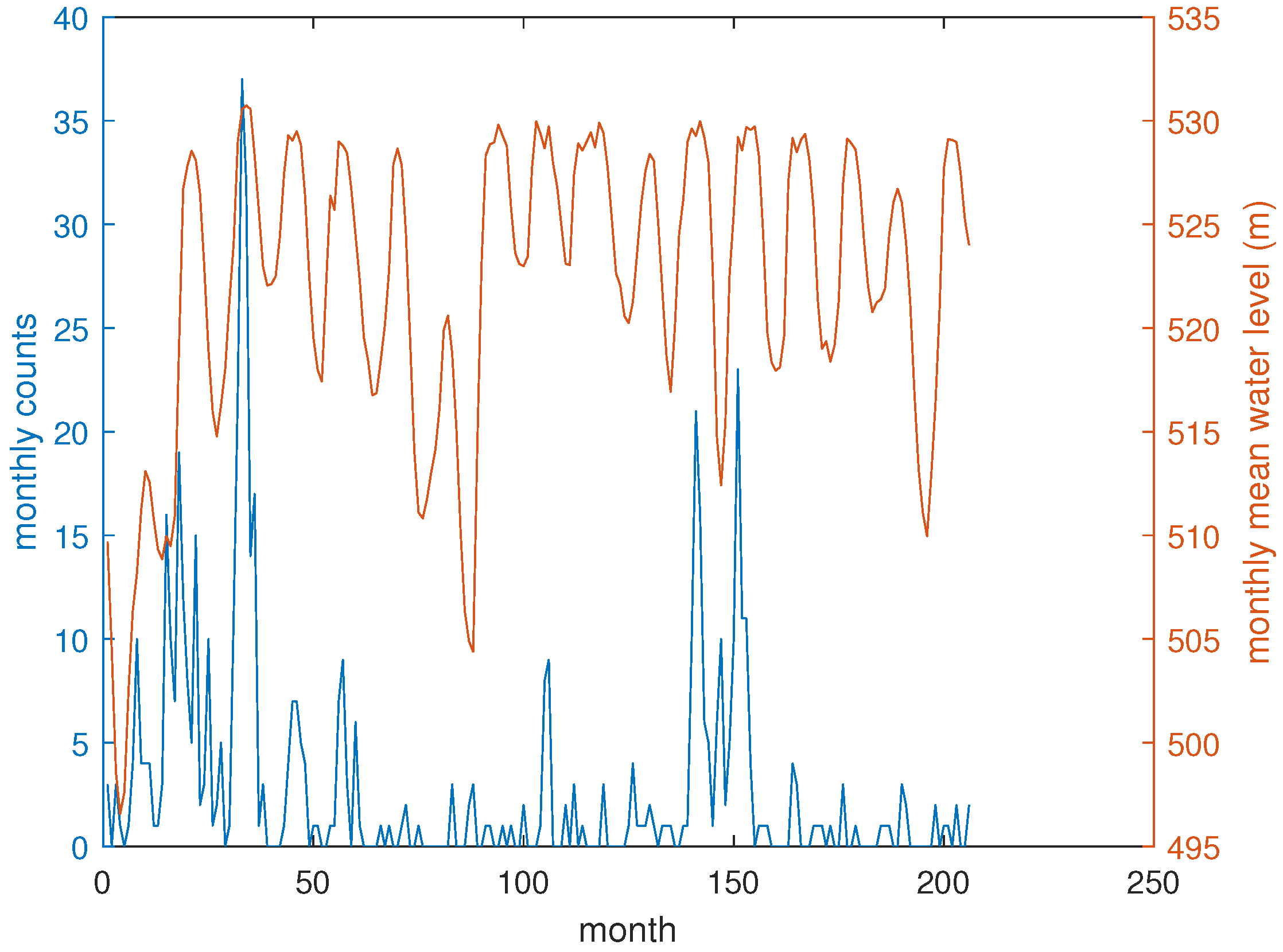
2. Seismotectonics of the High Agri Valley and Dataset Description

The High Agri Valley (HAV) is a quaternary intermontane basin located in the axial part of the Southern Apennines, hosting western Europe’s largest onshore oil reservoir. The latter is trapped in the Apulian carbonates by a system of wide anticlines: these developed during the upper Miocene-Early Pleistocene shortening phase experienced by the region and are overlaid by a thick tectonic melange composed of deeply deformed foredeep deposits [31,32]. The present geological and geomorphological configuration of the valley is dominated by two oppositely dipping, NW-trending systems of normal faults that developed in the Plio-Pleistocene regional extension: (1) the more recent Monti della Maddalena Fault System (MMFS), NE-dipping and bounding the valley to the southwest; (2) the more mature Eastern Agri Fault System (EAFS), SW-dipping and bounding the valley to the northwest. Both MMFS and EAFS are multi-segment arrays of faults running for approximately 25–30 km (Figure 1).

The HAV is currently affected by an ongoing tectonic activity as testified by stress indicators and geodetic and strain rate field data: the latter reveals an extension rate from 1 mm yr⁻¹ to 5 mm yr⁻¹. Furthermore, the study area is among the Mediterranean regions characterized by the strongest seismogenic potential, as witnessed by the 1857 M 7.1 Basilicata earthquake [33,34]. In the last 40 years, the HAV experienced only very low-magnitude earthquakes which very rarely exceed magnitude 3. The present natural seismicity mainly consists of small seismic events and earthquake sequences usually located at depths ranging between 8 km and 12 km (e.g., Castelsaraceno seismic sequence, [35]). In addition, the HAV seismicity is presently characterized by two clusters of events induced by human activities: (a) northeast of the artificial Pertusillo Lake, low-magnitude seismicity (ML < 2.0) is induced by the reinjection of coproduced formation water from oil reservoir exploitation via the Costa Molina 2 well [23,36]; (b) west of the Pertusillo reservoir, a cluster of low-magnitude seismicity (ML < 3) is associated with the annual pressure perturbations related to the 10–15 m water level fluctuations of the lake [25,27,37].

In this study, 1082 earthquakes located west of Pertusillo Lake, recorded between 2001 and 2018, were analyzed (Figure 2). The earthquake locations were determined by inverting 10,267 P-wave and 9390 S-wave arrival times, which were manually picked from the signals recorded by seismic stations belonging to several networks installed in the area. These include the private local network operated by ENI company [38], and the public seismic networks operating in the area such as the Italian National Seismic Network [39], the Irpinia Seismic Network [40], the HAVO network (formerly INSIEME) [41] and Geofon [42]. The earthquakes were in a 3-D velocity model of the area [38] using the probabilistic, non-linear, absolute earthquake location algorithm NonLinLoc [43]. On average, 18 seismic phases were used for locating the earthquakes, with values ranging from 4 to 68. The resulting earthquake locations are characterized by a median RMS value equal to 0.1 s and median horizontal and vertical location errors equal to 1.0 km and 1.3 km, respectively. The local magnitude of the located earthquakes was then computed using the Hutton and Boore relation [44], which is also employed by the Italian National Seismic Network [39].

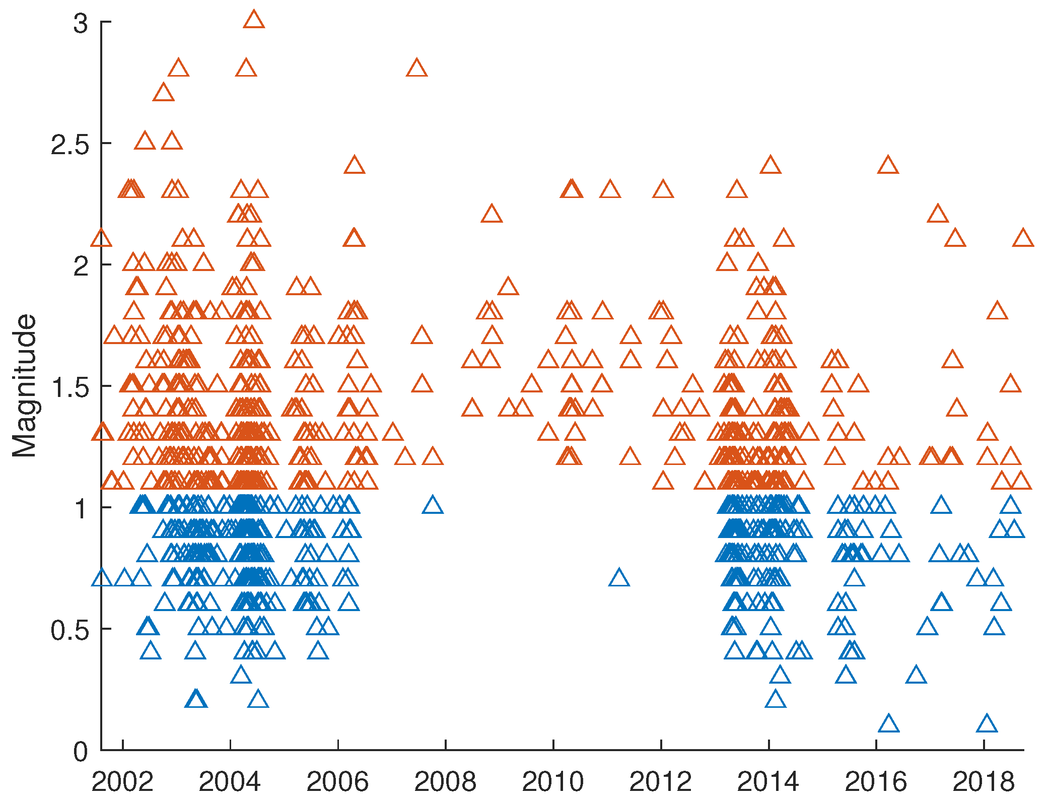
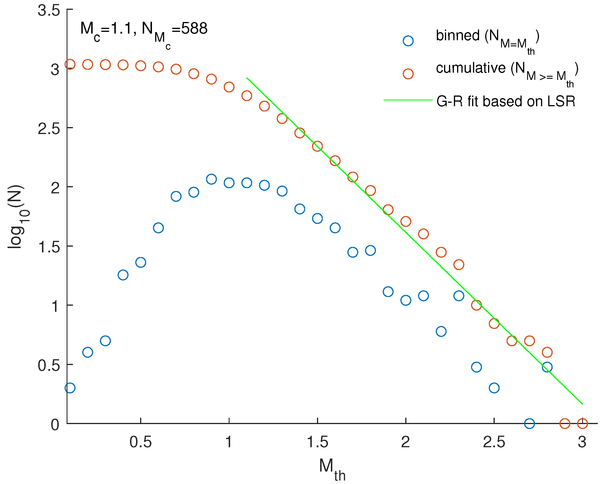
3. The Frequency–Magnitude Distribution

The frequency–magnitude distribution of earthquakes is generally fitted by the Gutenberg–Richter (GR) law [45] that is a relationship between the number N of earthquakes with magnitude $M\ge M_{th}$ and the magnitude threshold $M_{th}$ represented by $lo{g}_{10}N=a-b{M}_{th}$. The a-value represents the seismic productivity or seismic rate; thus, the larger the a, the larger the number of events. The b-value indicates the proportion of small events with respect to the large ones and informs on the stress crustal conditions; thus, a good and reliable estimation of the b-value is crucial for performing a reliable seismic hazard assessment [46,47,48,49,50].

Another important parameter to estimate when performing any statistical analysis of a seismic dataset is the estimation of the completeness magnitude $M_c$ that corresponds to the minimum magnitude above which all the seismic events are detected [51]. Thus, only the events with magnitude above or equal to $M_c$ are selected. There are several methods for estimating the $M_c$ [52,53,54,55]; in our study we used the maximum curvature method (MAXC) [52], where the completeness magnitude corresponds to the largest bin in the noncumulative frequency–magnitude distribution; however, [56] suggest to add 0.2 to the $M_c$ estimated by the MAXC method.

There are several methods to estimate the b-value; the most used ones are the least square linear regression (LSR) [57] and Aki’s method [58]. In our study, we used the LSR method (Supplementary File S1 shows the comparison between the LSR method and Aki’s method).

The LSR method is a curve-fitting technique that minimizes the summed squares of the residuals. Applying this procedure, the estimation of the b value is the following:

$$b={\displaystyle \frac{N{\sum }_{i=1}^N{M}_{\mathit{th},i}{log}_{10}{N}_{M\ge M_{\mathit{th},i}}-{\sum }_{i=1}^N{M}_{\mathit{th},\mathit{i}}{log}_{10}{N}_{M\ge M_{\mathit{th},i}}}{N{\sum }_{i=1}^N{\left(M_{\mathit{th},\mathit{i}}\right)}^2-{\left({\sum }_{i=1}^N{M}_{\mathit{th},\mathit{i}}\right)}^2}}.$$

(1)

where N represents the size of the earthquake dataset, and $N_{M\ge M_{th}}$ denotes the number of events with a magnitude $M\ge M_{th}$.

Figure 3 shows the frequency–magnitude distribution of the sequence of earthquakes under investigation. Applying the MAXC method [59] (consisting of taking the maximum of the binned frequency–magnitude distribution as the completeness magnitude) and incorporating a correction of 0.2 [56], the completeness magnitude was determined to be $M_C=1.1$. The b-value of the Gutenberg–Richter law, estimated using Equation (1), is 1.45. Consequently, after filtering for earthquakes with magnitudes $M\ge M_C$, the complete seismic catalog was reduced to 588 events (depicted as red triangles in Figure 2), which will serve as the basis for subsequent analyses.

4. Methods

4.1. The Global and Local Coefficient of Variation

The temporal clustering of an earthquake sequence can be analyzed using the following two coefficients of variation, $C_v$ [60] defined as

$$C_v={\displaystyle \frac{{\sigma }_T}{{\mu }_T}}$$

(2)

and $L_v$ [61] defined as

$$L_v={\displaystyle \frac{1}{N-1}}\sum _{i=1}^{N-1}3{\displaystyle \frac{{(T_i-T_{i+1})}^2}{{(T_i+T_{i+1})}^2}}$$

(3)

where $\{T_i,i=1,\dots ,N\}$ is the series of the interevent times and ${\sigma }_T$ and ${\mu }_T$ are their standard deviation and mean.

For seismic series, whose occurrence time is Poissonianly distributed, $C_v$ as well as $L_v$ range around 1. If the seismic sequence is periodic or quasi-periodic, both the coefficients of variations are smaller than 1. In the case of time-clusterized earthquake series, $C_v$ and $L_v$ are both larger than 1. $C_v$ is a global measure of the degree of clusterization of the seismic sequence and, thus, might be influenced by fluctuations of event rate. $L_v$ is a local measure of the stepwise variability of the interoccurrence intervals since it is quite independent of slow variation in average rate. For instance, a sequence obtained by joining two periodic sequences is characterized by $L_v=0$ (in fact, locally, it is periodic), but it is $C_v\gg 1$ because, globally, it appears strongly time-clusterized.

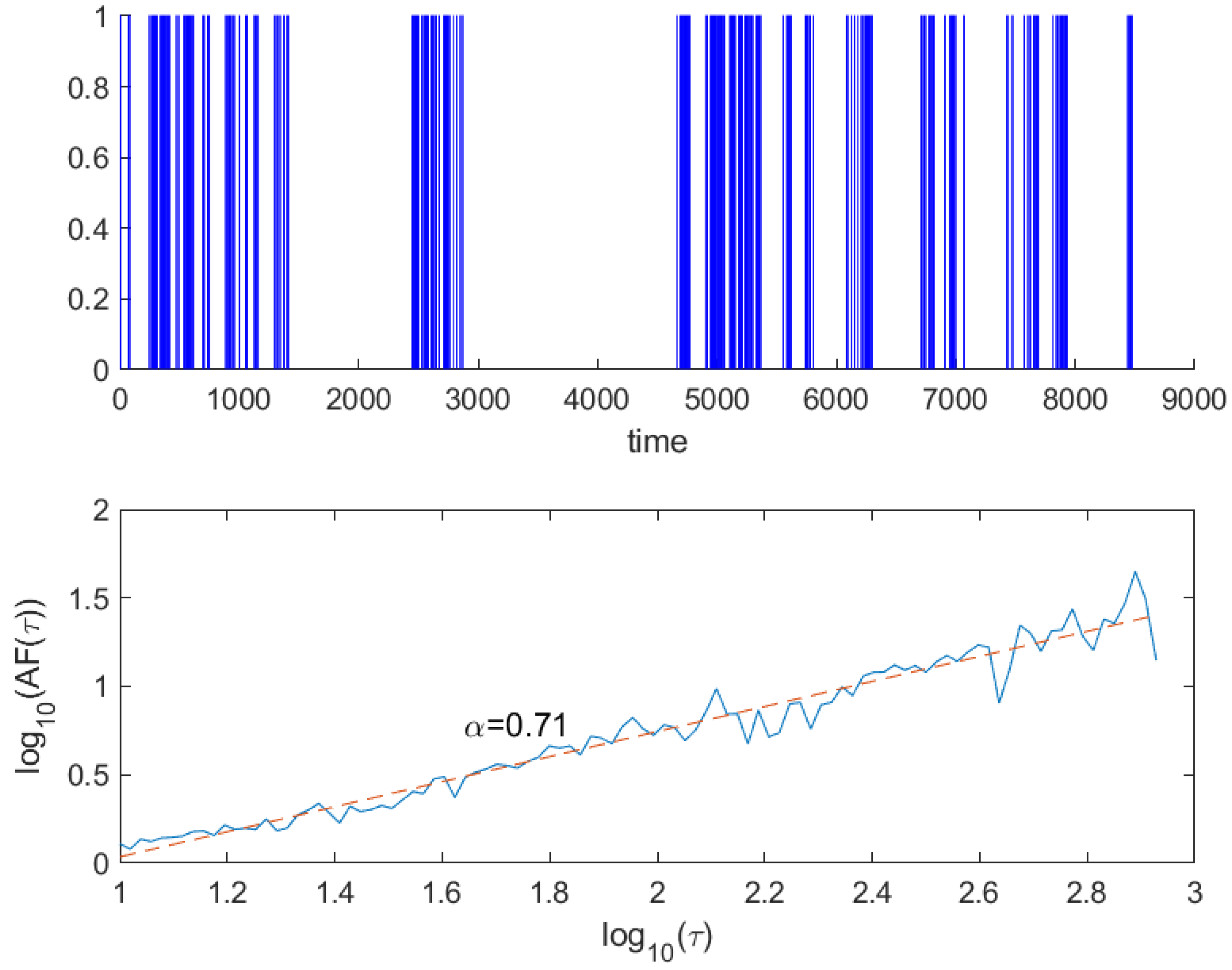
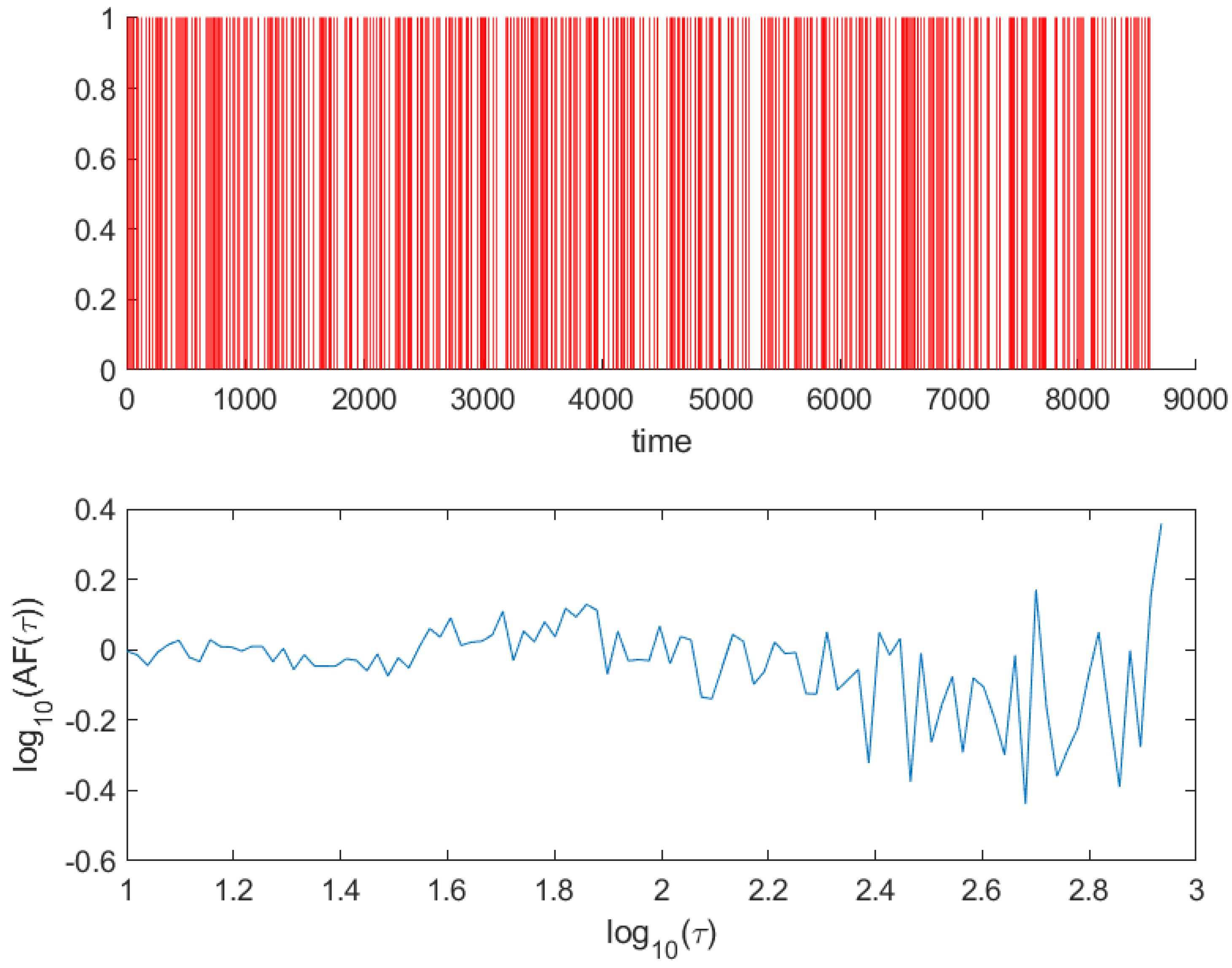
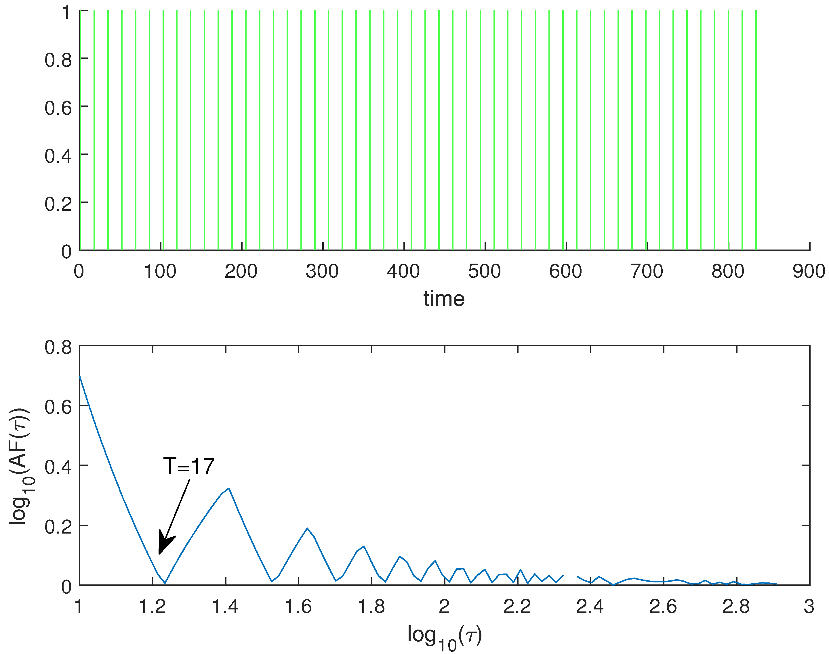
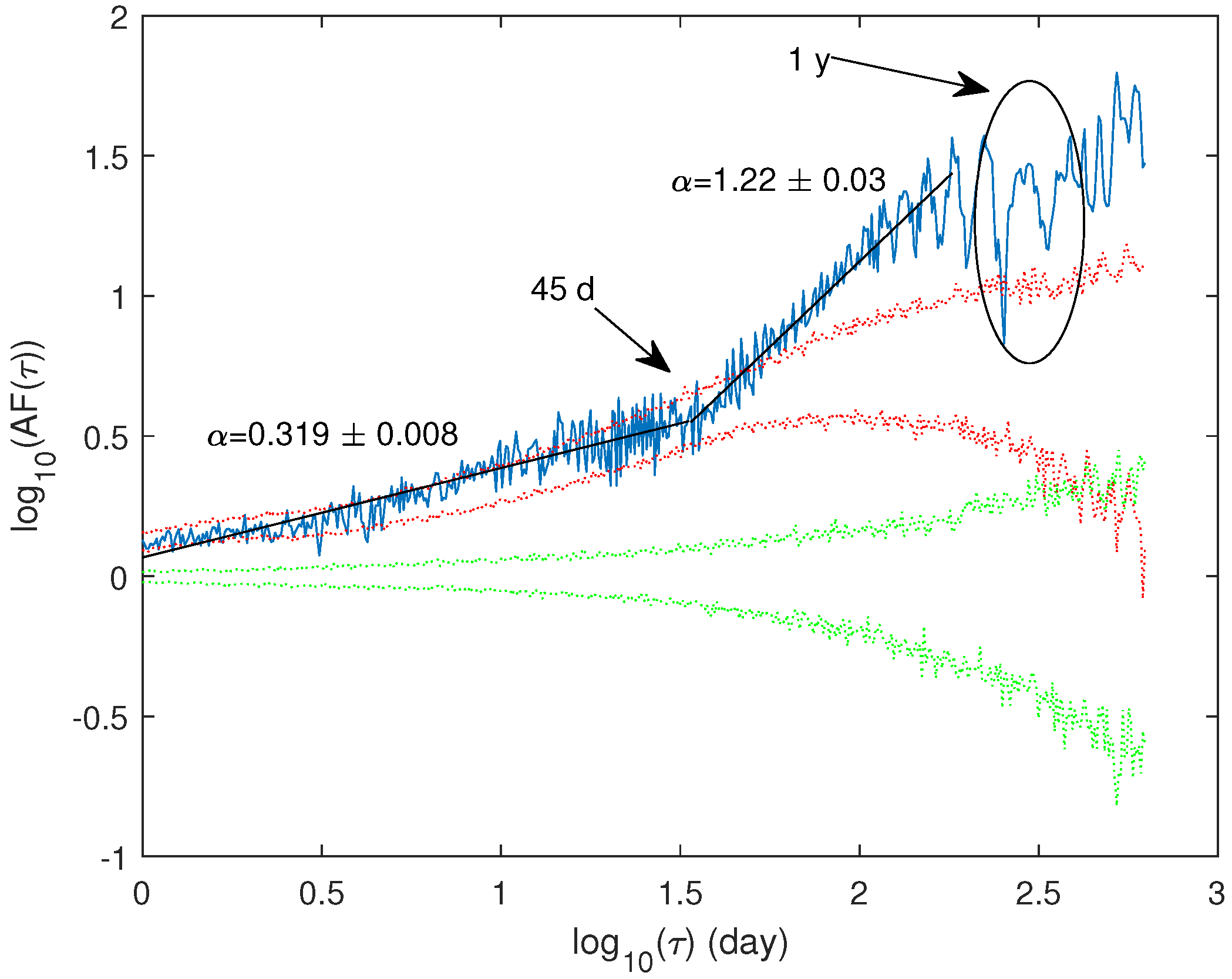
4.2. The Allan Factor

The Allan Factor (AF) is a fractal method used to reveal not only the existence of time-clusterized structures in earthquake sequence, similarly the global and local coefficients of variation, but also to identify the timescales where the sequence is time-clusterized. Dividing the time axis into equally spaced contiguous counting windows of duration $\tau$, which is the timescale, it is possible to construct the series of counts $\left\{N_k\left(\tau \right)\right\}$ that are the number of earthquakes falling in the k-th window [62]. The AF is defined by the following formula.

$$AF\left(\tau \right)={\displaystyle \frac{<{(N_{k+1}\left(\tau \right)-N_k\left(\tau \right))}^2>}{2<N_k\left(\tau \right)>}}$$

(4)

where the symbol $<..>$ indicates the average value. The AF has been used to investigate the time dynamics of a variety of natural phenomena [63,64]. A Poissonian sequence, whose events are uncorrelated and independent, is characterized by AF rather flat for all the investigated timescales assuming a value around 1 (except for very large timescales due to finite-size effects [65]); a clusterized sequence is, instead, characterized by AF changing with the timescale $\tau$; in particular, for a fractal (self-similar) sequence, the AF increases as power-law:

$$AF\left(\tau \right)\approx {\left({\displaystyle \frac{\tau }{{\tau }_0}}\right)}^{\alpha }.$$

(5)

The power-law exponent $\alpha$, called fractal exponent, quantifies the strength of time-clustering; ${\tau }_0$ is called fractal onset time and delimits the lower limit of significant scaling behavior in the AF [62]. Thus, if $\alpha \approx 0$, the earthquake sequence can be considered Poissonian, while if $\alpha >0$, it is clusterized. A drop of AF at a certain timescale indicates that the sequence is characterized by a periodicity of that timescale [66]. For a strictly periodic process, the AF tends toward zero as the timescale increases [66], with local minima occurring at timescales that are multiples of the primary period [67]. Consequently, the timescale at which the AF decreases corresponds to the periodicity.

For Poissonian point processes, where occurrence times are uncorrelated and independent, the probability density function of the interevent time, $p\left(T\right)$, follows a decaying exponential form, $p\left(T\right)=\lambda e^{-\lambda T}$, where $\lambda$ represents the mean rate of the process. Conversely, for clustered fractal point processes, $p\left(T\right)$ typically follows a power-law decay with the interevent time, expressed as $p\left(T\right)=k{T}^{-(1+\alpha )}$, where $\alpha$ is the aforementioned fractal exponent [62].

A seismic sequence is typically characterized by time-clustering, randomness, and periodicities. To analyze the time dynamics of a seismic sequence using the AF, we first examined how it behaves when applied to different types of point processes that can represent such sequences. Specifically, we considered three types of point processes: clusterized, Poissonian (random), and periodic. For each case, we simulated a point process with 500 events (consistent with the number of events in the earthquake sequences studied) and calculated the AF behavior for each.

Figure 4 (top panel) shows a simulated time-clusterized sequence generated with $\alpha =0.75$. The rate $\lambda$ of this process is ≈17, while its scaling exponent is ≈0.71, which is very close to the theoretical one. The scaling exponent is estimated by fitting the AF curve (bottom panel), plotted on log-log scales with a straight line, and calculating its slope using the least squares method. Figure 5 shows a simulated Poissonian sequence (top panel) with the same number of events as the clusterized at the same rate $\lambda$. The AF (bottom panel) is approximately flat, fluctuating around the value of 0. Figure 6 shows a periodic point process with period $T=\lambda =17$ (top panel). The AF (bottom panel) is characterized by a sequence of minima, the first one coinciding with the period of the sequence.

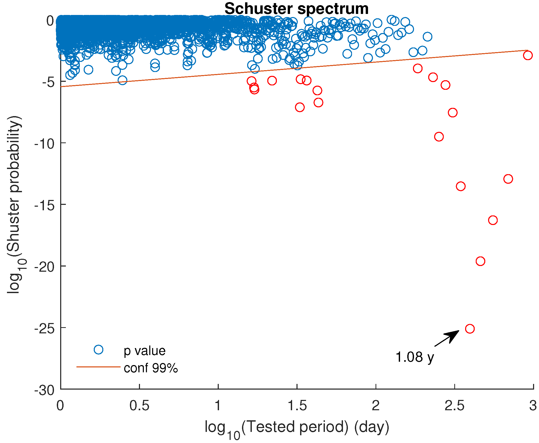
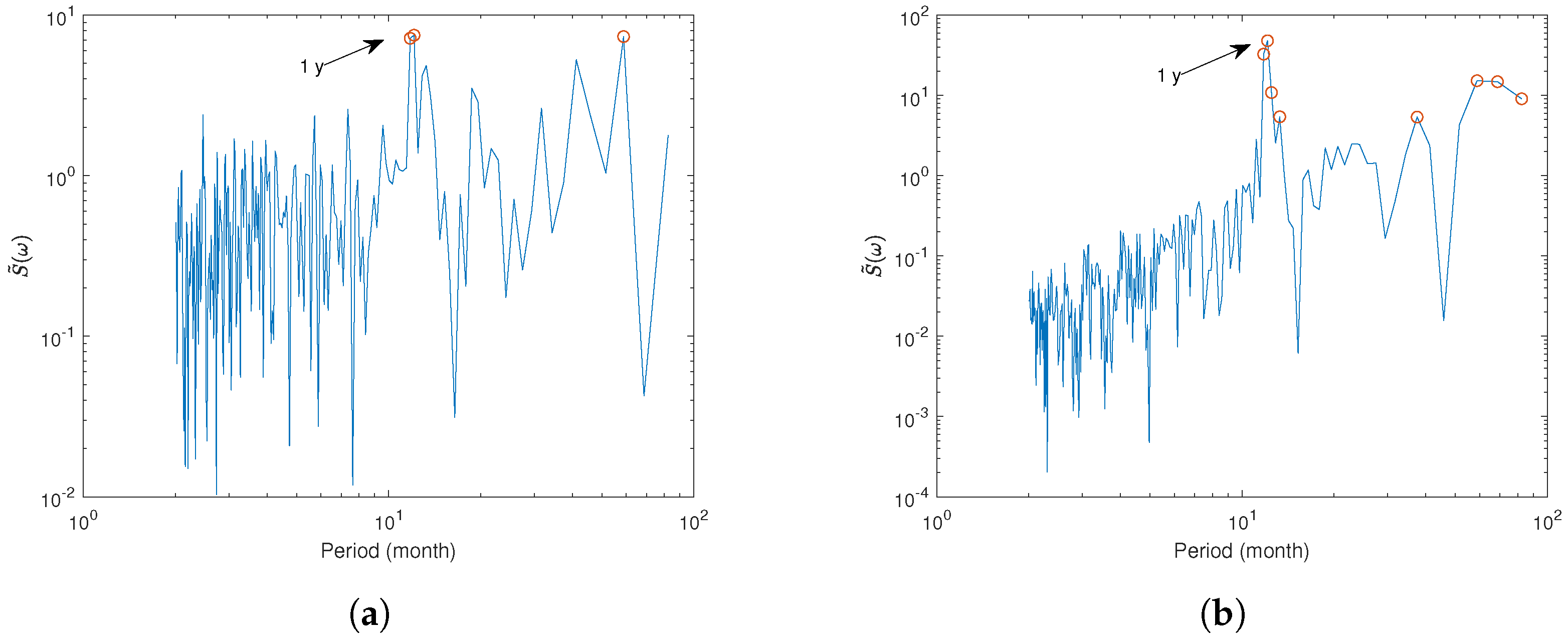
4.3. The Schuster’s Spectrum

The Schuster test was used to investigate tidal triggering [68] and reservoir-triggering [69] of seismicity. For a sinusoidal variation of seismic activity, supposing that the probability of occurrence times of earthquakes is a sinusoidal function of period T, to each occurrence time of the k-th earthquake $t_k$, a phase ${\theta }_k={\displaystyle \frac{2\pi t_k}{T}}$ can be associated, transforming the sequence of N occurrence times in a unit-length step 2-dimensional walk that changes direction with the phase ${\theta }_k$. If D is the distance between the starting and the ending points of this walk, the probability p that a distance larger than or equal to D can be reached by a uniformly distributed random 2-dimensional walk is the probability that the occurrence times $t_k$ are randomly originated by a uniform seismicity rate. This probability is called Schuster’s p-value, given by:

$$p=e^{-{\displaystyle \frac{D^2}{N}}}.$$

(6)

The lower the Schuster’s p-value, the larger the probability of a periodicity at period T. Indicating as $T_{min}$ and $T_{max}$ the minimum and the maximum of the periods to be tested, the number M of Schuster’s tests is given by [70,71]

$$M={\displaystyle \frac{t}{ϵ}}\left({\displaystyle \frac{1}{T_{min}}}-{\displaystyle \frac{1}{T_{max}}}\right).$$

(7)

where usually $ϵ=1$. As demonstrated in [70], a periodicity T will not be due to chance if its Schuster p-value is significantly lower than $T/t$.

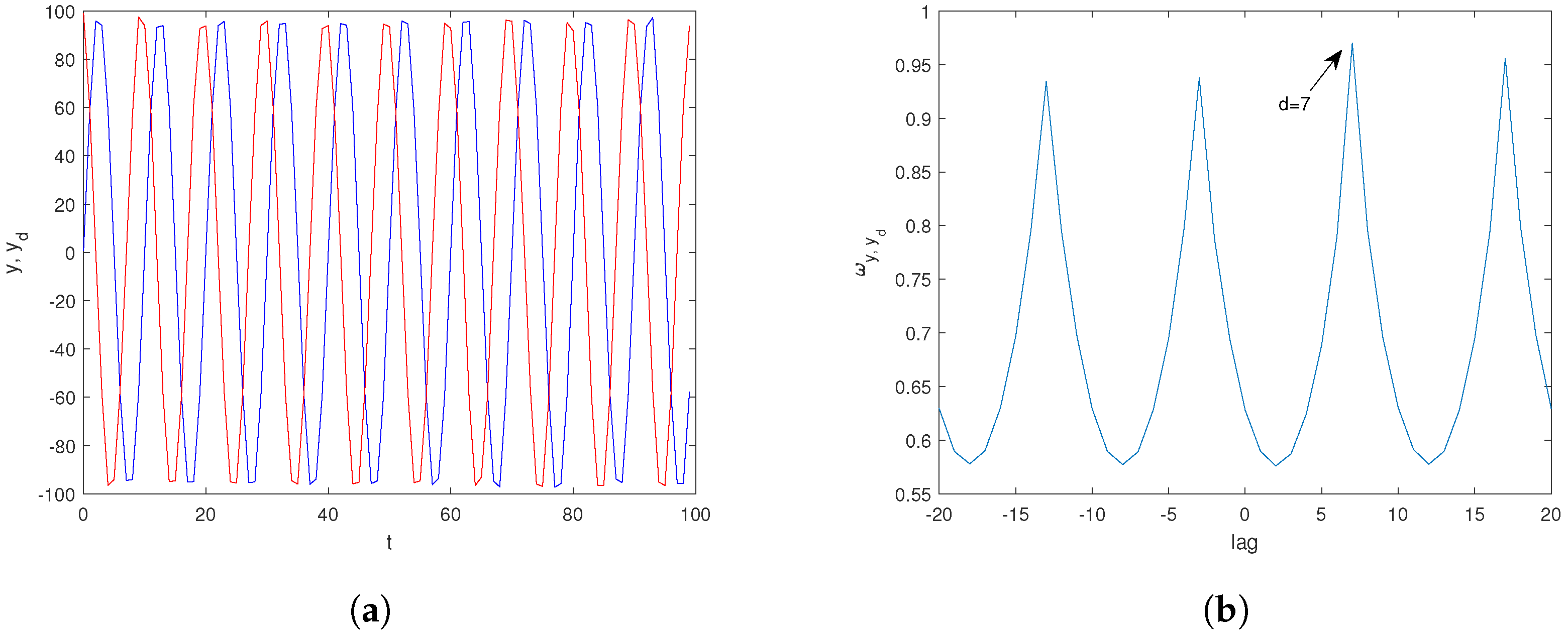
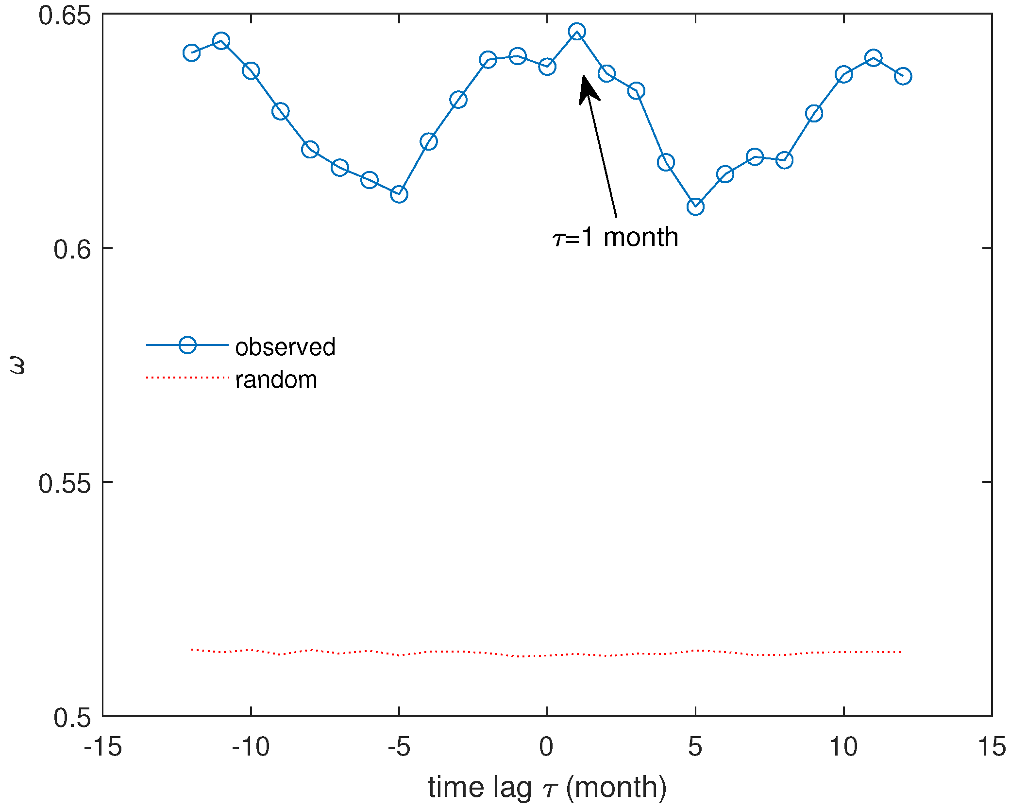
4.4. The Correlogram-Based Periodogram

Usually, the power spectrum of a time series $y_n$, for $n=0,\dots ,N-1$, where N is the length of the series, is estimated by the periodogram.

Considering the simple model of periodic series:

$$y_n=\beta cos(\omega t+\varphi )+{ϵ}_n$$

(8)

where $\beta >0$, $0<\omega <\pi$, $\varphi$ distributed as a uniform variable in $(-\pi ,\pi ]$, and ${ϵ}_n$ being a series of uncorrelated random variables with mean 0 and standard deviation $\sigma$, independent of $\varphi$.

The periodogram is given by

$$I\left(\omega \right)={\displaystyle \frac{1}{N}}|\sum _{n=1}^N{y}_n{e}^{-i\omega n}{|}^2,0\le \omega \le \pi$$

(9)

and it is calculated for

$${\omega }_l={\displaystyle \frac{2\pi l}{N}},l=0,1,\dots ,a$$

(10)

where $a=\left[{\displaystyle \frac{N-1}{2}}\right]$ and $\left[x\right]$ indicates the integer part of x. For a signal strongly modulated by a cycle with frequency ${\omega }_0$, the periodogram will be peaked at ${\omega }_0$. For an uncorrelated signal $(\beta =0)$, the periodogram will be uniformly distributed across the frequency range [72].

Ahdesmäki et al. [73] proposed the correlogram-based periodogram; this estimator detects more effective cycles in a series compared to the traditional periodogram. The periodogram $I\left(\omega \right)$ is equivalent to the correlogram

$$S\left(\omega \right)=\sum _{k=-N+1}^{N-1}\widehat{r}\left(k\right)e^{-i\omega k}$$

(11)

where

$$\widehat{r}\left(m\right)={\displaystyle \frac{1}{N}}\sum _{k=1}^{N-m}{y}_k{y}_{k+m}$$

(12)

is the estimator of the autocorrelation function. Using the sample autocorrelation function

$$\rho \left(m\right)={\displaystyle \frac{\frac{1}{N}{\sum }_{i=1}^N(x_i-\overline{x})(y_i-\overline{y})}{{\sigma }_x{\sigma }_y}}$$

(13)

where $\overline{x}$ indicates the mean, Ahdesmäki et al. [73] proposed the following correlogram-based periodogram to estimate the power spectrum of a series:

$$\tilde{S}\left(\omega \right)=2Re\left(\sum _{k=0}^L\tilde{\rho }\left(k\right)e^{-i\omega k}\right)-\tilde{\rho }\left(0\right).$$

(14)

where $Re\left(x\right)$ indicates the real part of x, N is the length of the series, $\tilde{\rho }\left(m\right)$ is the biased Spearman’s rank correlation coefficient. Contrarily to the standard periodogram, the correlogram-based periodogram can be negative; thus, the absolute value is considered. It was shown that the correlogram-based periodogram could be more effective than the traditional periodogram in estimating the power spectrum of short time series, even with only a few dozen samples [73].

To test a frequency ${\omega }_l$ the g-statistics can be used:

$$g={\displaystyle \frac{\left|\tilde{S}\left({\omega }_l\right)\right|}{{\sum }_{i=1}^a\left|\tilde{S}\left({\omega }_i\right)\right|}}.$$

(15)

A large g indicates a powerful frequency. The significance of the tested frequency can be analyzed by means of the simulation-based technique [73]: using Equation (8) we simulate random series, and each of them, we calculate the g-value by means of Equation (15). From all the obtained g-values, we estimate the distribution of g-statistics and then the p-value. A strong frequency of the series is identified by a low p-value.

4.5. The Visibility Graph

The Visibility Graph (VG) [74] converts a time series into a graph or network, whose nodes are given by the values of the series, and the links between them satisfy the following geometrical visibility rule:

$$y_c<y_b+(y_a-y_b){\displaystyle \frac{t_b-t_c}{t_b-t_a}},$$

(16)

where $t_a<t_c<t_b$. In practice, two values $y_a\left(t_a\right)$ and $y_b\left(t_b\right)$ are visible to each other if any other value $y_c\left(t_c\right)$ fulfils Equation (16). The VG method has been applied in several research fields, like economics [75,76,77], weather forecasting [78,79], medicine [80], oceanography [81], etc.

The adjacency matrix $A=\left\{a_{ij}\right\}$ is a mathematical representation used to describe the connections between nodes in a graph, and it is defined as follows:

$$a_{ij}=\left\{\begin{array}{c}1\mathrm{if}\mathrm{nodes}\mathrm{i}\mathrm{and}\mathrm{j}\mathrm{are}\mathrm{connected}\hfill \\ 0\mathrm{otherwise}\hfill \end{array}\right..$$

(17)

Thus, the adjacency matrix in a VG provides a way to encode the visibility relationships between values in a time series, indicating which values are directly visible to each other based on the visibility criterium (Equation (16)).

Considering two time series with adjacency matrices $A^1=\left\{a_{ij}^1\right\}$ and $A^2=\left\{a_{ij}^2\right\}$, the Average Edge Overlap (AEO) (defined in the context of the multivariate time series by [82,83,84]) is given by:

$${\omega }_{1,2}={\displaystyle \frac{{\sum }_i{\sum }_{j>i}{\sum }_{\nu =1}^2{a}_{ij}^{\nu }}{M{\sum }_i{\sum }_{j>i}\left(1-{\delta }_{0,{\sum }_{\nu =1}^2{a}_{ij}^{\nu }}\right)}}.$$

(18)

where ${\delta }_{0,{\sum }_{\nu =1}^2{a}_{ij}^{\nu }}$ is the Kronecker delta. ${\omega }_{1,2}$ can vary between 1 (when both the adjacency matrices are identical) and ${\displaystyle \frac{1}{2}}$ (when each edge exists just for one VG); we can view these two conditions like the maximum of correlation and the absence of correlation among the variables, respectively.

The AEO defined in Equation (18) can be used to estimate the time lag between two series. Given two time series $\left\{x_t\right\}$ and $\left\{y_t\right\}$, keeping the first fixed, we construct the time-shifted copies of the second one, $\left\{y_{t-{\tau }_1}\right\},\left\{y_{t-{\tau }_2}\right\},\left\{y_{t-{\tau }_3}\right\},\dots$ For $\left\{x_t\right\}$ and each of the time-shifted copies of $\left\{y_t\right\}$, we calculate the adjacency matrix, obtained by applying Equation (16). Indicating as $A^x$ the adjacency matrix of $x_t$ and as $A_{{\tau }_1}^y$, $A_{{\tau }_2}^y$, $A_{{\tau }_3}^y$, etc. the adjacency matrices of the delayed copies of $y_t$, from the maximum of sequence $\left\{{\omega }_{x,y}\left({\tau }_1\right)\right),{\omega }_{x,y}\left({\tau }_2\right)),{\omega }_{x,y}\left({\tau }_3\right))\dots \}$ the time lag between the series $\left\{x_t\right\}$ and $\left\{y_t\right\}$ can be derived. As an example, consider two sinusoids, $y\left(t\right)=100sin\left({\displaystyle \frac{2\pi t}{10}}\right)$ and $y_d\left(t\right)=100sin\left({\displaystyle \frac{2\pi (t-7)}{10}}\right)$; both have a period of $T=10$, while the second one is delayed by $d=7$ (Figure 7a). Plotting ${\omega }_{y,y_d}$ between the two sinusoids, the maximum is at $\tau =7$, which is exactly the delay of the second sinusoid with respect to the first one (Figure 7b). Even when the sinusoids are corrupted by random noise, ${\omega }_{y,y_d}$ effectively captures the delay between them. Specifically, Figure 8a illustrates $y\left(t\right)=100sin\left({\displaystyle \frac{2\pi t}{10}}\right)+w(0,300)$ and $y_d\left(t\right)=100sin\left({\displaystyle \frac{2\pi (t-7)}{10}}\right)+w(0,70)$, where $w(0,300)$ and $w(0,70)$ represent white noise with $\mu =0$ and variances ${\sigma }^2=300$ and ${\sigma }^2=70$, respectively. The $AEO$ correctly identifies the delay at lag $\tau =7$, as shown in Figure 8b.

5. Results and Discussion

We analyzed the seismicity of the Pertusillo area (southern Italy) from August 2001 to September 2019 (Figure 2). The number of events in the complete seismic dataset is 588.

Considering the series of the interevent times, we found $C_v=2.58$ and $L_v=1.30$. The 95% confidence intervals of these estimates were calculated by generating 1000 surrogate Poissonian earthquake sequences with the same number of events and the same mean interevent time of the original one; they are $\left[0.92,1.08\right]$ for $C_v$ and $\left[0.91,1.09\right]$ for $L_v$, where the left and right extremes of each interval are the 2.5th and 97.5th percentiles of the distribution of $C_v$ and $L_v$ calculated for the Poissonian surrogates. As can be seen, the earthquake series that occurred in the Pertusillo area is time-clusterized on both global and local scales, being their values well beyond the 95% confidence interval.

Figure 9 shows the AF for the investigated seismicity and the 95% confidence band in relationship with two types of surrogate sequences: 1000 Poissonian sequences with the same rate as the original one (green), and 1000 random sequences obtained by randomly shuffling the interevent times of the original one (red), keeping, then, the same probability density function of the interevent times $p\left(\tau \right)$. The AF increases with the timescale $\tau$, and this means that the Pertusillo seismicity is time-clusterized. The AF is well beyond the Poissonian 95% confidence, and this indicates that it is significantly non-Poissonian at all the investigated timescales. However, the AF is within the 95% confidence band based on 1000 random shuffles of the interevent times up to about 45 days; this indicates that the clustering behavior might depend on the $p\left(\tau \right)$ up to the timescale of about 45 days; while for larger timescales it is independent of the $p\left(\tau \right)$. Around the timescale of 1 year, the AF is characterized by a drop that is evidence of the existence of yearly periodic fluctuations of the time dynamics. Two distinct scaling regions are discernible in the log-log plot of the AF: the first encompasses shorter timescales, up to approximately 45 days, exhibiting a scaling exponent $\alpha \approx 0.32$; the second region spans longer timescales, exceeding 45 days, with a scaling exponent $\alpha \approx 1.22$. The presence of two different scaling regions indicates the co-existence of two different mechanisms that govern the time dynamics of the seismic process at two different timescale ranges. The increase in the scaling exponent $\alpha$ for timescales exceeding ≈45 days highlights a prolonged clustering of seismicity, indicative of swarm-like earthquake distributions, in contrast to short-term clustering typical of mainshock-aftershock sequences. This behavior is consistent with the protracted reservoir-induced nature of seismicity, driven by stress perturbations associated with seasonal fluctuations in the water level of the Pertusillo reservoir.

Figure 10 shows the Schuster’s spectrum. For each tested period ranging from 1 day to half of the entire period of investigation, the p-value (circles) was calculated; some periods have a p-value below the 95% confidence line (red circles). Among these, the period corresponding to the lowest p-value is about 1 year; this is in agreement with the previous AF result and signals the presence of annual periodicity in the time dynamics of the earthquakes.

The time series of monthly earthquake counts with magnitudes equal to or above the completeness magnitude, $M_c$, exhibits an oscillatory behavior resembling that of the monthly mean water level (Figure 11). The correlogram-based periodogram (CBP) for both variables is displayed in Figure 12. In the CBPs, periods significant at the 95% confidence level are marked with hollow circles. Among these significant peaks, the most prominent occurs at 1 year for both variables. The coherence observed between the two CBPs suggests a relationship between the two variables at a yearly timescale, highlighting the role of water level fluctuation as a driving force behind the seismicity rate variation in the area.

We applied the VG to both monthly time series and calculated the AEO varying the time lag $\tau$ between −12 and 12 months. The obtained values of $\omega$ are above 0.5 for all $\tau$.

To assess the significance of the obtained $\omega$ values, we generated a null distribution representing the case where no correlation exists between the two graphs. This distribution was created using a permutation-based approach, which follows these steps: (1) The positions of the elements in the adjacency matrices of both graphs are randomly permuted while preserving the null elements on the diagonal and maintaining symmetry. These constraints ensure that node connections are randomly shuffled while preserving the overall graph structure consistent with the VG rules; (2) The $\omega$ is calculated for each permutation and for each time lag $\tau$; (3) After performing this process 100 times, a distribution of $\omega$ values under the null hypothesis is obtained for each time lag $\tau$; (4) For each $\tau$, the 95th percentile of the corresponding distribution is calculated; (5) By enveloping these percentiles, a 95% confidence curve for the $\omega$ is constructed. If the observed $\omega$ exceeds this curve, it is considered statistically significant.

Figure 13 shows the observed $\omega$ between the monthly counts and the monthly mean water level as a function of $\tau$, along with the 95% confidence curve. The figure clearly demonstrates that the correlation between the two time series is significant for all time lags $\tau$. Notably, the maximum value of $\omega$ occurs at $\tau =1$, suggesting that the monthly mean water level leads the monthly earthquake counts by approximately one month (±0.5 months, given the monthly resolution of the time series). This finding supports the hypothesis that the dominant perturbation mechanism of the Pertusillo Lake on fault activation, already critically stressed by the tectonic stress field, is not the immediate undrained elastic response to loading but a delayed seismic response due to diffusion of pore fluid pressures.

The only open question to be answered that may justify a delay of $1.0\pm 0.5$ months of the monthly earthquake counts with respect to the monthly water level time series is the role of aquifers, whose recharges generally can have a temporal delay of up to 1 month with respect to the Pertusillo water level loading depending on the aquifers’ depth and the hydraulic conductivity of porous media through which water flows downward. By observing that some events in the period 2013–2015 were located northeast of the Pertusillo Lake (Figure 1), Picozzi et al. [28] already suggested that the triggering process of the northernmost located events could be potentially ascribed to aquifers. However, their role could be only investigated through simulations using numerical models due to the lack of information on aquifers in the study area.

6. Conclusions

In this study, we examined the temporal dynamics of instrumental seismic activity in the vicinity of the Pertusillo reservoir (Southern Italy) from 2001 to 2018. Our primary objective was to explore the time-dependent behavior of the seismicity using fractal and spectral analysis methods. The earthquakes in the investigated area exhibit time-clustered behavior, with a superimposed periodic cycle of approximately 1 year. Additionally, the application of the topological method of the Visibility Graph revealed a connection between seismicity and the reservoir’s water level, with the water level leading the earthquake-triggering process with a delay of 1.0 ± 0.5 months. These findings provide robust statistical evidence that the seismic activity in the Pertusillo reservoir area may be of the protracted reservoir-triggered type with a delayed response due to pore-pressure diffusion. While we encourage future studies to explore the potential role of aquifers through simulations, this study provides strong evidence that variations in the water level of the reservoir could be a driving force behind the observed seismicity for the whole investigation period.

We also emphasize the robustness and potential applicability of our methodology to other reservoir regions, as it relies solely on seismicity data and water level records. However, its broad applicability may be limited by factors such as catalog incompleteness (e.g., a limited number of detected events caused by the sensitivity of the seismic monitoring network, restricted spatial and temporal coverage, event misclassification, and errors in earthquake location and magnitude estimates) in other regions or the lack of detailed information on the reservoir.

Despite these considerations, our study highlights the novelty of integrating fractal, spectral, and topological analyses to better understand the temporal dynamics of continued reservoir-induced seismicity without requiring additional assumptions or datasets.

References

1. Moein, M.; Langenbruch, C.; Schultz, R.; Grigoli, F.; Ellsworth, W.; Wang, R.; Rinaldi, A.; Shapiro, S. The physical mechanisms of induced earthquakes. Nat. Rev. Earth Environ. 2023, 4, 847–863. [Google Scholar] [CrossRef]
2. Saar, M.; Manga, M. Seismicity induced by seasonal groundwater recharge at Mt. Hood, Oregon. Earth Planet. Sci. Lett. 2003, 214, 605–618. [Google Scholar] [CrossRef]
3. Shapiro, S.A. Fluid-Induced Seismicity; Cambridge University Press: Cambridge, UK, 2015; p. 298. [Google Scholar]
4. King, G.; Stein, R.; Lin, J. Static stress changes and the triggering of earthquakes. Bull. Seismol. Soc. Am. 1994, 84, 935–953. [Google Scholar]
5. Harris, R. Introduction to special section: Stress triggers, stress shadows, and implications for seismic hazard. J. Geophys. Res. 1998, 103, 24347–24358. [Google Scholar] [CrossRef]
6. Stokes, S.M.; Ge, S.; Brown, M.R.M.; Menezes, E.A.; Sheehan, A.F.; Tiampo, K.F. Pore pressure diffusion and onset of induced seismicity. J. Geophys. Res. 2023, 128, e2022JB026012. [Google Scholar] [CrossRef]
7. Gupta, H.K.; Rastogi, B.K. Dams and Earthquakes; Elsevier: Amsterdam, The Netherlands, 1976; p. 229. [Google Scholar]
8. Tao, W.; Masterlark, T.; Shen, Z.K.; Ronchin, E. Impoundment of the Zipingpu reservoir and triggering of the 2008 Mw 7.9 Wenchuan earthquake, China. J. Geophys. Res. Solid Earth 2015, 120, 7033–7047. [Google Scholar] [CrossRef]
9. Wilson, M.P.; Foulger, G.R.; Gluyas, J.G.; Davies, R.J.; Julian, B.R. HiQuake: The human-induced earthquake database. Seismol. Res. Lett. 2017, 88, 1560–1565. [Google Scholar] [CrossRef]
10. Wilkinson, M.; Mhana, N.; Wilson, M.P.; Foulger, G.R.; Tezel, T.; Gluyas, J.G. The plausibility of claimed induced seismicity. Sci. Rep. 2024, 14, 30846. [Google Scholar] [CrossRef]
11. Chen, R.; Zhu, J.; Li, S.; Zhang, S.; Chen, X.; Li, Q.; Wang, P.; Zhang, J.; Dai, L.; Jia, Y. Characteristics and mechanisms of human-induced earthquakes in China from the QuakeQuake database. Geol. J. 2023, 58, 2099–2131. [Google Scholar] [CrossRef]
12. Roeloffs, E.A. Fault stability changes induced beneath a reservoir with cyclic variations in water level. J. Geophys. Res. 1988, 93, 2107–2124. [Google Scholar]
13. Bell, M.L.; Nur, A. Strength changes due to reservoir-induced pore pressure and stresses and application to Lake Oroville. J. Geophys. Res. 1978, 83, 4469–4483. [Google Scholar] [CrossRef]
14. Simpson, D.W.; Leith, W.S.; Scholz, C.H. Two types of reservoir-induced seismicity. Bull. Seismol. Soc. Am. 1988, 78, 2025–2040. [Google Scholar]
15. Carder, D. Seismic investigations in the Boulder Dam area, 1940–1944, and the influence of reservoir loading on earthquake activity. Bull. Seismol. Soc. Am. 1945, 35, 175–192. [Google Scholar] [CrossRef]
16. Stabile, T.A.; Fat-Helbary, E.R.; Serlenga, V.; Panebianco, S.; Tizzani, P.; Castaldo, R.; Telesca, L.; El-Amin, E.M.; Hamed, A. Fault structure and earthquake clustering in Aswan region (Egypt) revealed by high-precision earthquake location from 35 years of recorded natural and induced seismicity. Earth Planet. Sci. Lett. 2024, 642, 118881. [Google Scholar] [CrossRef]
17. Dura-Gomez, I.; Talwani, P. Hydromechanics of the Koyna-Warna region, India. Pure Appl. Geophys. 2010, 167, 183–213. [Google Scholar] [CrossRef]
18. Goswami, D.; Akkiraju, V.V.; Roy, S. Heat flow and thermal structure in the Koyna seismic zone, western India: Implications for recurrent reservoir triggered seismicity. Tectonophysics 2024, 873, 230216. [Google Scholar] [CrossRef]
19. Simpson, D.; Negmatullaev, S. Induced seismicity at Nurek Reservoir, Tadjikistan, USSR. Bull. Seismol. Soc. Am. 1981, 71, 1561–1586. [Google Scholar] [CrossRef]
20. Talwani, P. On the nature of reservoir-induced seismicity. Pure Appl. Geophys. 1997, 150, 473–492. [Google Scholar] [CrossRef]
21. Gupta, H. A review of recent studies of triggered earthquakes by artificial water reservoirs with special emphasis on earthquakes in Koyna, India. Earth Sci. Rev. 2002, 58, 279–310. [Google Scholar] [CrossRef]
22. Valoroso, L.; Improta, L.; Chiaraluce, L.; DiStefano, R.; Ferranti, L.; Govoni, A.; Chiarabba, C. Active faults and induced seismicity in the Val d’Agri area (southern Apennines, Italy). Geophys. J. Int. 2009, 178, 488–502. [Google Scholar] [CrossRef]
23. Stabile, T.A.; Giocoli, A.; Perrone, A.; Piscitelli, S.; Lapenna, V. Fluid injection induced seismicity reveals a NE dipping fault in the southeastern sector of the High Agri Valley (southern Italy). Geophys. Res. Lett. 2014, 41, 5847–5854. [Google Scholar] [CrossRef]
24. Stabile, T.A.; Giocoli, A.; Perrone, A.; Piscitelli, S.; Telesca, L.; Lapenna, V. Relationship between seismicity and water level of the Pertusillo reservoir (southern Italy). Boll. Geofis. Teor. Appl. 2015, 56, 505–517. [Google Scholar] [CrossRef]
25. Telesca, L.; Giocoli, A.; Lapenna, V.; Stabile, T.A. Robust identification of periodic behavior in the time dynamics of short seismic series: The case of seismicity induced by Pertusillo Lake, southern Italy. Stoch. Environ. Res. Risk Assess. 2015, 29, 1437–1446. [Google Scholar] [CrossRef]
26. Vlček, J.; Eisner, L.; Stabile, T.A.; Telesca, L. Temporal Relationship Between Injection Rates and Induced Seismicity. Pure Appl. Geophys. 2018, 175, 2821–2835. [Google Scholar] [CrossRef]
27. Rinaldi, A.; Improta, L.; Hainzl, S.; Catalli, F.; Urpi, L.; Wiemer, S. Combined approach of poroelastic and earthquake nucleation applied to the reservoir-induced seismic activity in the Val d’Agri area, Italy. J. Rock Mech. Geotech. Eng. 2020, 12, 802–810. [Google Scholar] [CrossRef]
28. Picozzi, M.; Serlenga, V.; Stabile, T.A. Spatio-temporal evolution of ground motion intensity caused by reservoir-induced seismicity at the Pertusillo artificial lake (southern Italy). Front. Earth Sci. 2022, 10, 1048196. [Google Scholar] [CrossRef]
29. Barkat, A.; Tan, Y.J.; Madson, A. Deciphering the Interplay between Reservoir Loading and Dynamic Stresses at the Pertusillo Reservoir. Seismol. Res. Lett. 2024, 96, 461–472. [Google Scholar] [CrossRef]
30. Lavecchia, A.; Serlenga, V.; Filippucci, M.; Stabile, T.A.; Prosser, G.; Tallarico, A. Fault (re)activation and fluid-induced seismicity: An example from the Val d’Agri intermontane basin (southern Italy). J. Geophys. Res. Solid Earth 2024, 129, e2024JB028710. [Google Scholar] [CrossRef]
31. Mazzoli, S.; Barkham, S.; Cello, G.; Gambini, R.; Mattioni, L.; Shiner, P.; Tondi, E. Reconstruction of continental margin architecture deformed by the contraction of Lagonegro Basin, southern Apennines, Italy. J. Geol. Soc. 2001, 158, 309–319. [Google Scholar]
32. Shiner, P.; Beccaccini, A.; Mazzoli, S. Thin-skinned versus thick-skinned structural models for Apulian carbonate reservoirs: Constraints from the Val d’Agri Fields, S Apennines, Italy. Mar. Petrol. Geol. 2004, 21, 805–827. [Google Scholar]
33. Mallet, R. Great Neapolitan Earthquake of 1857. The First Principles of Observational Seismology; Traduzione italiana in Ferrari G.: London, UK, 1862. [Google Scholar]
34. Rovida, A.; Antonucci, A. EPICA-European PreInstrumental Earthquake Catalogue, Version 1.1; Istituto Nazionale di Geofisica e Vulcanologia (INGV): Roma, Italy, 2021. [Google Scholar] [CrossRef]
35. Panebianco, S.; Serlenga, V.; Satriano, C.; Cavalcante, F.; Stabile, T.A. Semi-automated template matching and machine-learning based analysis of the August 2020 Castelsaraceno microearthquake sequence (southern Italy). Geomat. Nat. Hazards Risk 2023, 14, 2207715. [Google Scholar] [CrossRef]
36. Stabile, T.A.; Vlček, J.; Wcisło, M.; Serlenga, V. Analysis of the 2016–2018 fluid-injection induced seismicity in the High Agri Valley (Southern Italy) from improved detections using template matching. Sci. Rep. 2021, 11, 20630. [Google Scholar] [CrossRef]
37. Stabile, T.A.; Giocoli, A.; Lapenna, V.; Perrone, A.; Piscitelli, S.; Telesca, L. Evidence of low-magnitude continued reservoir-induced seismicity associated with the Pertusillo artificial lake (southern Italy). Bull Seism. Soc. Am. 2014, 104, 1820–1828. [Google Scholar] [CrossRef]
38. Serlenga, V.; Stabile, T.A. How do local earthquake tomography and inverted dataset affect earthquake locations? The case study of High Agri Valley (Southern Italy). Geomat. Nat. Hazards Risk 2019, 10, 49–78. [Google Scholar] [CrossRef]
39. Eni spa. VAL D’AGRI NETWORK. [Data Set]. 2001. Available online: https://www.fdsn.org/networks/detail/VA/ (accessed on 31 January 2025).
40. INGV. Rete Sismica Nazionale (RSN); Istituto Nazionale di Geofisica e Vulcanologia (INGV): Roma, Italy, 2005. [Google Scholar] [CrossRef]
41. Stabile, T.A.; Serlenga, V.; Satriano, C.; Romanelli, M.; Gueguen, E.; Gallipoli, M.R.; Ripepi, E.; Saurel, J.M.; Panebianco, S.; Bellanova, J.; et al. The INSIEME seismic network: A research infrastructure for studying induced seismicity in the high Agri Valley (southern Italy). Earth Syst. Sci. Data 2020, 12, 519–538. [Google Scholar] [CrossRef]
42. GEOFON Data Centre. GEOFON Seismic Network; GFZ Data Services: Potsdam, Germany, 1993. [Google Scholar] [CrossRef]
43. Lomax, A.; Virieux, J.; Volant, P.; Berge, C. Probabilistic earthquake location in 3D and layered models: Introduction of a Metropolis-Gibbs method and comparison with linear locations. In Advances in Seismic Event Location; Thurber, C.H., Rabinowitz, N., Eds.; Kluwer: Amsterdam, The Netherlands, 2000; pp. 101–134. [Google Scholar]
44. Hutton, L.; Boore, D.M. The ML scale in southern California. Bull. Seismol. Soc. Am. 1987, 77, 2074–2094. [Google Scholar]
45. Gutenberg, R.; Richter, C. Frequency of earthquakes in California. Bull. Seismol. Soc. Am. 1944, 34, 185–188. [Google Scholar]
46. Scholz, C.H. The frequency-magnitude relation of microfracturing in rock and its relation to earthquakes. Bull. Seismol. Soc. Am. 1968, 58, 399–415. [Google Scholar]
47. Wyss, M. Towards a physical understanding of the earthquake frequency distribution. Geophys. J. R. Astron. Soc. 1973, 31, 341–359. [Google Scholar]
48. Amitrano, D. Brittle-ductile transition and associated seismicity: Experimental and numerical studies and relationship with the b value. J. Geophys. Res. 2003, 108, 2044. [Google Scholar] [CrossRef]
49. Gulia, L.; Wiemer, S. The influence of tectonic regimes on the earthquake size distribution: A case study for Italy. Geophys. Res. Lett. 2010, 37, 10305. [Google Scholar] [CrossRef]
50. Godano, C.; Petrillo, G. Estimating the Completeness Magnitude m and the b-Values in a Snap. Earth Space Sci. 2023, 10, e2022EA002540. [Google Scholar] [CrossRef]
51. Rydelek, P.A.; Sacks, I.S. Testing the completeness of Earthquake catalogs and the hypothesis of self-similarity. Nature 1989, 337, 251–253. [Google Scholar] [CrossRef]
52. Wiemer, S.; Wyss, M. Minimum magnitude of completeness in earthquake catalogs: Examples from Alaska, the Western United States, and Japan. Bull. Seismol. Soc. Am. 2000, 90, 859–869. [Google Scholar]
53. Cao, A.; Gao, S.S. Temporal variation of seismic b-values beneath northeastern Japan island arc. Geophys. Res. Lett. 2002, 29, 48-1–48-3. [Google Scholar] [CrossRef]
54. Ogata, Y.; Katsura, K. Analysis of temporal and spatial heterogeneity of magnitude frequency distribution inferred from earthquake catalogues. Geophys. J. Int. 1993, 113, 727–738. [Google Scholar] [CrossRef]
55. Godano, C. A new method for the estimation of the completeness magnitude. Phys. Earth Planet. Inter. 2017, 263, 7–11. [Google Scholar] [CrossRef]
56. Woessner, J.; Wiemer, S. Assessing the Quality of Earthquake Catalogues: Estimating the Magnitude of Completeness and Its Uncertainty. Bull. Seismol. Soc. Am. 2005, 95, 684–698. [Google Scholar] [CrossRef]
57. Kařník, V.; Klíma, K. Magnitude-frequency distribution in the European-Mediterranean earthquake regions. Tectonophysics 1993, 220, 309–323. [Google Scholar] [CrossRef]
58. Aki, K. Maximum likelihood estimate of b in the formula log(N) = abM and its confidence limits. Bull. Earthq. Res. Inst. Univ. Tokyo 1965, 43, 237–239. [Google Scholar]
59. Mignan, A.; Woessner, J. Estimating the magnitude of completeness for earthquake catalogs. Community Online Resour. Stat. Seism. Anal. 2012, 1–45. [Google Scholar] [CrossRef]
60. Kagan, Y.Y.; Jackson, D.D. Long-Term Earthquake Clustering. Geophys. J. Int. 1991, 104, 117–134. [Google Scholar] [CrossRef]
61. Shinomoto, S.; Miura, K.; Koyama, S. A measure of local variation of inter-spike intervals. Biosystems 2005, 79, 67–72. [Google Scholar] [CrossRef] [PubMed]
62. Thurner, S.; Lowen, S.B.; Feurstein, M.C.; Heneghan, C.; Feichtinger, H.G.; Teich, M.C. Analysis, synthesis, and estimation of fractal-rate stochastic point processes. Fractals 1997, 5, 565–596. [Google Scholar] [CrossRef]
63. Telesca, L.; Cuomo, V.; Lapenna, V.; Macchiato, M. Statistical analysis of fractal properties of point processes modelling seismic sequences. Phys. Earth Planet. Int. 2001, 125, 65–83. [Google Scholar] [CrossRef]
64. Telesca, L.; Amatulli, G.; Lasaponara, R.; Lovallo, M.; Santulli, A. Time-scaling properties in forest-fire sequences observed in Gargano area (southern Italy). Ecol. Model. 2005, 185, 531–544. [Google Scholar] [CrossRef]
65. Telesca, L.; ElShafey Fat ElBary, R.; Amin Mohamed, A.E.E.; ElGabry, M. Analysis of the cross-correlation between seismicity and water level in the Aswan area (Egypt) from 1982 to 2010. Nat. Hazards Earth Syst. Sci. 2012, 12, 2203–2207. [Google Scholar] [CrossRef]
66. Gebber, G.L.; Orer, H.S.; Barman, S.M. Fractal Noises and Motions in Time Series of Presympathetic and Sympathetic Neural Activities. J. Neurophysiol. 2006, 95, 1176–1184. [Google Scholar] [CrossRef]
67. Serinaldi, F.; Kilsby, C.G. On the sampling distribution of Allan factor estimator for a homogeneous Poisson process and its use to test inhomogeneities at multiple scales. Phys. A Stat. Mech. Its Appl. 2013, 392, 1080–1089. [Google Scholar] [CrossRef]
68. Tanaka, S.; Sato, H.; Matsumura, S.; Ohtake, M. Tidal triggering of earthquakes in the subducting Philippine Sea plate beneath the locked zone of the plate interface in the Tokai region, Japan. Tectonophysics 2006, 417, 69–80. [Google Scholar] [CrossRef]
69. Telesca, L.; Tsereteli, N.; Chelidze, T.; Lapenna, V. Spectral Investigation of the Relationship between Seismicity and Water Level in the Enguri High Dam Area (Georgia). Geosciences 2024, 14, 22. [Google Scholar] [CrossRef]
70. Ader, T.J.; Avouac, J.P. Detecting periodicities and declustering in earthquake catalogs using the Schuster spectrum, application to Himalayan seismicity. Earth Planet. Sci. Lett. 2013, 377–378, 97–105. [Google Scholar] [CrossRef]
71. Ader, T.J.; Lapusta, N.; Avouac, J.P.; Ampuero, J.P. Response of rate-and-state seismogenic faults to harmonic shear-stress perturbations. Geophys. J. Int. 2014, 198, 385–413. [Google Scholar] [CrossRef]
72. Priestley, M.B. Spectral Analysis and Time Series; Academic Press: London, UK; New York, NY, USA, 1981; p. 890. [Google Scholar]
73. Ahdesmäki, M.; Lähdesmäki, H.; Pearson, R.; Huttunen, H.; Yli-Harja, O. Robust detection of periodic time series measured from biological systems. BMC Bioinform. 2005, 6, 117. [Google Scholar]
74. Lacasa, L.; Luque, B.; Ballesteros, F.; Luque, J.; Nuno, J.C. From time series to complex networks: The visibility graph. Proc. Natl. Acad. Sci. USA 2008, 105, 4972–4975. [Google Scholar] [PubMed]
75. Zhang, R.; Ashuri, B.; Shyr, Y.; Deng, Y. Forecasting construction cost index based on visibility graph: A network approach. Phys. A Stat. Mech. Its Appl. 2018, 493, 239–252. [Google Scholar]
76. Long, Y. Visibility graph network analysis of gold price time series. Phys. A Stat. Mech. Its Appl. 2013, 392, 3374–3384. [Google Scholar]
77. Wang, N.; Li, D.; Wang, Q. Visibility graph analysis on quarterly macroeconomic series of China based on complex network theory. Phys. A Stat. Mech. Its Appl. 2012, 391, 6543–6555. [Google Scholar] [CrossRef]
78. Jiang, W.; Wei, B.; Zhan, J.; Xie, C.; Zhou, D. A visibility graph power averaging aggregation operator: A methodology based on network analysis. Comput. Ind. Eng. 2016, 101, 260–268. [Google Scholar]
79. Chen, S.; Hu, Y.; Mahadevan, S.; Deng, Y. A visibility graph averaging aggregation operator. Phys. A Stat. Mech. Its Appl. 2014, 403, 1–12. [Google Scholar]
80. Yu, M.; Hillebrand, A.; Gouw, A.A.; Stam, C.J. Horizontal visibility graph transfer entropy (HVG-TE): A novel metric to characterize directed connectivity in large-scale brain networks. NeuroImage 2017, 156, 249–264. [Google Scholar] [CrossRef] [PubMed]
81. Telesca, L.; Lovallo, M.; Pierini, J.O. Visibility graph approach to the analysis of ocean tidal records. Chaos. Solit. Fractals. 2012, 45, 1087–1091. [Google Scholar] [CrossRef]
82. Lacasa, L.; Nicosia, V.; Latora, V. Network structure of multivariate time series. Sci. Rep. 2015, 5, 15508. [Google Scholar] [PubMed]
83. Bianchi, F.M.; Livi, L.; Alippi, C.; Jenssen, R. Multiplex visibility graphs to investigate recurrent neural network dynamics. Sci. Rep. 2017, 7, 44037. [Google Scholar] [CrossRef]
84. Carmona-Cabezas, R.; Gómez-Gómez, J.; Ariza-Villaverde, A.B.; Gutiérrez de Ravé, E.; Jiménez-Hornero, F.J. Multiplex Visibility Graphs as a complementary tool for describing the relation between ground level O3 and NO2. Atmos. Pollut. Res. 2020, 11, 205–212. [Google Scholar]
Figure 1. Map view of the seismicity catalog analyzed in this study, comprising 1082 earthquakes recorded between 2001 and 2018, located west of Pertusillo Lake. Earthquake locations were determined using a 3-D velocity model. The figure also includes a schematic representation of the two main NW-trending fault systems bordering the valley: the NE-dipping Monti della Maddalena Fault System (MMFS) to the southwest and the SW-dipping Eastern Agri Fault System (EAFS) to the northwest.
Fractalfract 09 00208 g001
Figure 2. Earthquake time distribution. The red triangles represent the earthquakes above the completeness magnitude (see text).
Fractalfract 09 00208 g002
Figure 3. Binned (blue) and cumulative (red) frequency–magnitude distribution. The green line represents the Gutenberg–Richter fit based on the least square linear regression method.
Fractalfract 09 00208 g003
Figure 4. Simulated fractal point process with the theoretical value of α = 7.5 .
Fractalfract 09 00208 g004
Figure 5. Simulated Poisson point process with the same rate as the fractal process shown in Figure 4.
Fractalfract 09 00208 g005
Figure 6. Periodic point process with period identical to the rate of the fractal process shown in Figure 4.
Fractalfract 09 00208 g006
Figure 7. (a) Comparison between two sinusoids: y ( t ) = 100 sin 2 π t 10 (blue) and y d ( t ) = 100 sin 2 π ( t 7 ) 10 (red), both with period T = 10 and the second one delayed by d = 7 . (b) Variation of ω y , y d with the time lag τ ; the maximum indicates the time lag of d = 7 between the two sinusoids.
Fractalfract 09 00208 g007
Figure 8. (a) Comparison between two sinusoids: y ( t ) = 100 sin 2 π t 10 + w ( 0 , 300 ) (blue) and y d ( t ) = 100 sin 2 π ( t 7 ) 10 + w ( 0 , 70 ) (red), both with period T = 10 and the second one delayed by d = 7 . (b) Variation of ω y , y d with the time lag τ ; the maximum indicates the time lag of d = 7 between the two sinusoids.
Fractalfract 09 00208 g008
Figure 9. Allan Factor for the investigated seismicity (blue) along with the 95% Poissonian (green) and shuffle (red) confidence band. The two scaling regions are fitted by regression lines at small and large timescales with a crossover at about 45 days.
Fractalfract 09 00208 g009
Figure 10. Schuster’s spectrum.
Fractalfract 09 00208 g010
Figure 11. Time series of the monthly mean water level and volume (red) compared with that of the earthquake counts (blue).
Fractalfract 09 00208 g011
Figure 12. Correlogram-based periodogram of the monthly earthquake counts (a) and mean water level (b).
Fractalfract 09 00208 g012
Figure 13. Average edge overlap ω versus the time lag τ . The red dotted line represents the 95% confidence curve.
Fractalfract 09 00208 g013
Disclaimer/Publisher’s Note: The statements, opinions and data contained in all publications are solely those of the individual author(s) and contributor(s) and not of MDPI and/or the editor(s). MDPI and/or the editor(s) disclaim responsibility for any injury to people or property resulting from any ideas, methods, instructions or products referred to in the content.