Cost-Benefit and Dynamical Investigation of a Fractional-Order Corruption Population Dynamical System

Abstract

The main objective of this study was to investigate the effects of control measures on the diffusion of corruption in the population using a fractional order approach with optimal control theory and cost-benefit analysis. The associated fractional order optimal control problem using three time-dependent control measures was reformulated. Qualitative analysis of the model investigated the model solutions that exist uniquely, the equilibrium points and their stabilities, and the corruption threshold number. Furthermore, we utilized Pontryagin’s Maximum Principle to determine the optimal solution’s existence for the fractional order optimal control problem. Through completing numerical simulations, the study also verified the theoretical results and showed that the implementation of all the proposed control measures greatly reduced corruption diffusion in the community. Eventually, the cost-effectiveness investigation proved that strategy 1, which entailed implementing protection control measures, was the most cost-effective control strategy suggested to the stakeholders for reducing and managing the corruption diffusion problem in the population.

1. Introduction

It is difficult to conceptualize corruption from a social science standpoint because it can apply to a wide range of social activities and actions that will or will not be considered morally or even legally repugnant, depending on a specific set of cultural factors or beliefs [1]. However, according to other academics, corruption is an unpleasant and damaging behavior committed by people, such as unlawful gratitude, abusing a public position for personal benefit, or misusing public authority for one’s benefit [2,3]. It is a cancer for political, social, and economic reform and is sometimes referred to as a “worm inside the body of society” [4]. From the beginning of human history to the present time, corruption has been considered one major unavoidable social disease and has been associated with human being interactions [5]. It has been a socio-economic phenomenon or social threat that is rarely visible and is difficult to measure; however, theoretical discussions have tackled this phenomenon with enthusiasm but, due to the lack of firsthand real data, have rarely produced substantial results [6,7]. From minor violations or acts of unlawful remuneration to extensive mass theft by public authorities, corruption is a multifaceted topic and also has a significant negative impact on sustainable development and is known to cause inefficiencies, diversion of basic resources, and inequality as a result of such impacts [8,9]. The historical and cultural backgrounds of nations throughout the world have made great contributions to the intensity of corruption diffusion [10]. Since low corruption levels are related to high levels of institutional and social trust, the terms corruption and institutional quality play a fundamental role in a country’s socioeconomic development and overall welfare [11,12,13].

To develop the data and test their theories, sociologists who investigate the curse of corruption need to have a thorough understanding of history, society, language, and impacts from at least one intricate and detailed illustration [14]. The following conditions can be identified as mechanisms by which to mitigate corruption, even though complete eradication remains unattainable: a strong commitment to governance coupled with a spiritual engagement in the advancement of national and bureaucratic objectives; effective administration, along with suitable structural reforms within governmental frameworks and regulations to minimize the emergence of corruption; favorable historical and sociological contexts; the establishment of a robust anti-corruption value system; leadership from influential groups characterized by high moral and intellectual integrity; and a well-informed public capable of critically evaluating and responding to unfolding events [14].

Numerous scholars have developed and examined mathematical models pertaining to system dynamics in a variety of fields, such as the natural sciences, social sciences, and other fields [15,16]. While some studies have used fractional order derivatives, such as investigations [17,18], others have used integer order modeling, such as studies [19], to study real-world scenarios. Since its initial construction and analysis in 1975, the mathematical modeling of corruption has drawn the attention of numerous scholars due to its detrimental effects on society [5]. The diffusion of corruption has been the subject of numerous mathematical model studies, including [4,20,21]. We reviewed a number of studies in order to develop and evaluate our suggested fractional-order corruption diffusion model.

The rationale behind reviewing these studies was to determine the fundamental ideas of mathematical modeling, theories, methods, and methodologies, as well as to pinpoint any gaps or limitations. A six-compartmental fractional order optimal control problem for corruption diffusion dynamics was developed and examined by Bonyah Ebenezer [5]. The study did not conduct a cost-effectiveness analysis or divide the compromised individuals into two groups: ignorant and aware. Using optimum control strategies, Athithan et al. [21] investigated a corruption dissemination dynamical system. The cost-benefit of their suggested controlling activities was not evaluated, and their model, the standard SIR model, did not consider the different corruption statuses of people, such as their aware and unaware status. Danford, Oscar [22], “Corruption dynamics in Tanzania: Modeling the effects of control strategies”. A deterministic corruption diffusion dynamical system that considered the possible optimal control activities was developed and examined by Fantaye et al. [23]. Both the cost-benefit investigation of their suggested control activities and the different corruption statuses of individuals, such as their aware and unaware status, were not considered by their model. The study’s conclusions demonstrated that the best way to stop corruption from spreading was through prevention and punishment. An epidemiological corruption model with an immunity clause in Nigeria was developed and studied by Gweryina et al. [20]. Although they conducted both qualitative and quantitative analysis, they did not carry out a cost-benefit investigation. To investigate a corruption issue throughout the community, the study carried out by Alemneh et al. [24] investigated a corruption diffusion dynamical system with controlling activities. An investigation of cost-effectiveness was not conducted in their study. Tesfaye et al. [25] developed and examined the diffusion dynamics of stochastic corruption with transient immunity. Their four-class approach omitted cost-effectiveness analysis and optimum control theory. A dynamical system for corruption diffusion that took media coverage into consideration was developed and examined by Birhanu et al. [4]. Since their model took into account the effect of media coverage, it is unique when compared to other studies in the field. It did not, however, carry out cost-effectiveness analysis or optimal control. According to what we learned from the literature evaluation, no other researcher built a corruption diffusion dynamical system that takes into consideration both the conscious and uninformed classes. This study’s distinctiveness is ensured by the fact that it completed the cost-benefit for the proposed control activities investigation.

Our proposed study’s primary goal is to use a fractional order derivative approach in conjunction with the optimum control principle and cost-benefit investigation to examine how the proposed control measures affect the corruption diffusion problem. By taking into account three time-dependent regulating strategies, this paper primarily examines the corruption optimal control dynamical system with a fractional order derivatives approach. Additionally, there are corrupted and unaware and corrupted and aware subgroups within the human population of the corrupted group. Preventing corruption and improving the lives of those who are corrupted, both aware and unaware, are the controlling methods that we took into consideration. In order to investigate the most cost-benefit control activity to reduce and control the corruption diffusion, we numerically simulated the reconstructed control problem and conducted a cost-effectiveness investigation. The following parts comprise the remaining portion of this work: Section 2 defines the basic concepts of fractional calculus; Section 3 formulates and analyzes the fractional order model for corruption diffusion; Section 4 reformulates the fractional order control problem; Section 5 presents the results of the numerical simulation; Section 6 provides the cost-benefit investigation; and Section 7 concludes and provides future directions for the proposed study.

2. Fractional Calculus Concepts

Fundamental ideas in calculus in fractional form: The development of the suggested corruption diffusion dynamical system depends on the following basic definitions.

Definition 1.

Let $g\in C^n$ be a continuous function, then the φ’s Caputo fractional order derivative is defined by ^C$D_t^{\phi }g\left(t\right)={\displaystyle \frac{1}{\Gamma \left(n-\phi \right)}}{\int }_0^t{g}^n(\xi ){\displaystyle \frac{{(t-\xi )}^{n-\phi }}{t-\xi }}d\xi$, $n-1<\phi \le n\in N$ [26,27,28], where

$${}^{\mathrm{C}}D_t^{\phi }g\left(t\right)\mathrm{tends} \mathrm{to} \dot{g}\left(t\right)\mathrm{as} \phi \to 1.$$

Definition 2.

Let $g\in C^n$ be a function; consequently, the Caputo integral with a fractional order φ > 0 is defined as ^C$I_t^{\phi }g\left(t\right)={\displaystyle \frac{1}{\Gamma \left(\phi \right)}}{\int }_0^{t}f(\xi ){\displaystyle \frac{{(t-\xi )}^{\vartheta }}{t-\xi }}d\xi$, $0<\phi <1, t>0$ [5,26].

Definition 3.

Suppose ${\beta }_1>0,{\beta }_2>0$, then the function defined by $E_{{\beta }_1{,\beta }_2}\left(t\right)=\sum _{m=1}^{\infty }{\displaystyle \frac{t^m}{\Gamma \left({\beta }_{1}m+{\beta }_2\right)}}$ is known as a Mittag-Leffler approach function [8,25,29].

Definition 4.

Suppose ${\beta }_2=1$, then the Mittag-Leffler function is represented by $E_{{\beta }_1,1}\left(t\right)=\sum _{m=1}^{\infty }{\displaystyle \frac{t^m}{\Gamma \left({\beta }_{1}m+1\right)}}=E_{{\beta }_1}\left(t\right)$ [26].

Definition 5.

The stationary point for the Caputo-fractional order dynamical system is described by the constant $\theta \ast$ such that C$D_t^{\vartheta }\theta \left(t\right)=g\left(t,\theta \left(t\right)\right),\vartheta \in \left[\mathrm{0,1}\right]$ whenever $g\left(t,{\theta }^{\ast }\right)=0.$

Proposition 1.

Let φ$,$ for k $-1<\phi \le k$,$k\in N$ be the order of the derivative, then the Laplace transform is represented by $L\left(D_t^{\phi }h\right)\left(s\right)=s^{\phi }H\left(s\right)-\sum _{k=1}^{n-1}{s}^{\phi -k-1}{h}^k(0)$ such that $H\left(s\right)$, where $h\left(t\right)$ is the function in the Laplace transform approach.

Proposition 2.

For the two constants approach, the Mittag-Leffler case’s Laplace transformation is represented by $L\left(t^{{\beta }_2-1} E_{{\beta }_1,{\beta }_2}(\pm \gamma t^{{\beta }_1})\right)\left(s\right)={\displaystyle \frac{s^{{\beta }_1{\beta }_2}}{s^{{\beta }_1}\mp \gamma }}$.

Proposition 3.

Let $h(t)\in \mathcal{L}[0,T]$ and ^C$D_t^{\phi }h(t)\in \mathcal{L}[0,T]$ for φ$\in (\mathrm{0,1}]$, the Generalized Mean Value condition describes that  $h\left(t\right)=h\left(0\right)+{\displaystyle \frac{1}{\Gamma (\phi )}}$^C$D_t^{\phi }h(\zeta )t^{\phi }$ at $\zeta \in [0,t]$, at each point of time $t$, which satisfies $0<t\le T$.

Lemma 1.

From the third proposition mentioned above, we have the following approaches: (a) $h$ is not decreasing for all $t\in [0,T]$, if ^C$D_t^{\phi }h(t)\ge 0$, and (b) $h$ is not increasing for all $t\in [0,T]$, if ^C$D_t^{\phi }h(t)\le 0.$

Proposition 4.

Let us assume $f(t)\in L^{\infty }(\mathbb{R})\cap \mathcal{F}(\mathbb{R})$ and $\phi \in \mathbb{R},$ k $-1<\phi \le k, k\in N$ then the three criteria listed below are true (a). (^C$D_t^{\phi }{I}^{\phi }f)\left(t\right)=f\left(t\right)$, (b). $(I^{\phi }$ ^C$D_t^{\phi }f)\left(t\right)=f\left(t\right)-\sum _{j=0}^{k-1}{\displaystyle \frac{t^j}{j!}}{f}^j(0)$, (c). Particularly, if $0<\phi <1$, then $(I^{\phi }$ ^C$D_t^{\phi }f)\left(t\right)=f\left(t\right)-f(0)$, and (d). For a constant function $f\left(t\right)=b$ then ^C$D_t^{\phi }\left(b\right)=0.$

3. Formulation of Corruption Diffusion Fractional Order Model

3.1. Descriptions and Fundamental Assumptions

We divide the total population $N(t)$ at any time $t$ into five different groups in order to formulate the proposed corruption diffusion dynamical system for the corruption diffusion dynamics in the community that are considered in this study. These groups are as follows: people who are at risk for corruption are represented by $S(t)$; people who are exposed to corruption are represented by $E(t);$ people who are corrupted but unaware are represented by $U(t);$ people who are corrupted and aware are represented by $A(t);$ and people who are repented (improved) from corruption are represented by $R(t).$

$$N\left(t\right)=S\left(t\right)+E \left(t\right)+U \left(t\right)+A\left(t\right)+R\left(t\right).$$

(1)

The susceptible individuals become corrupted at the rate represented by

$${\mathsf{\lambda }}_{\mathrm{C}}\left(\mathrm{t}\right)={\displaystyle \frac{\mathsf{\beta }}{N}}\left({\mathsf{\rho }}_1{M}_C\left(t\right)+{\mathsf{\rho }}_2{H}_C\left(t\right)\right),$$

(2)

where ${\mathsf{\rho }}_1$ and ${\mathsf{\rho }}_2$ are parameters that reveal the corruptness of unaware and aware people, respectively.

➢

A $q$ portion of people who are exposed to corruption moves to the compartment $A(t)$ at $\varpi$, and the remaining part $(1-q$) enters into $U(t)$ with a similar rate.

➢

Some people from the unaware corrupted group $U(t)$ and from the $A(t)$ group progress into the group $R(t)$ at rates ${\alpha }_1$ and ${\alpha }_2$, respectively.

➢

The parameter $\eta$ is the rate of progression for unaware corrupted people to become aware of corruption.

➢

People in each compartment (group) homogeneously mix; i.e., they have the same corruption status.

➢

The total population is not constant.

➢

Fear of punishment is used as a mechanism for reducing corruption.

➢

Some protection mechanisms of corruption diffusion include: A strong commitment to governance coupled with a spiritual engagement in the advancement of national and bureaucratic objectives; effective administration along with suitable structural reforms within governmental frameworks and regulations to minimize the emergence of corruption; favorable historical and sociological contexts; the establishment of a robust anti-corruption value system; leadership from influential groups characterized by high moral and intellectual integrity; and a well-informed public capable of critically evaluating and responding to unfolding events.

➢

Corrupted individuals improve from corrupted activities due to fear of punishment, education mechanisms, and legal actions taken by the concerned body, etc.

➢

Some of the individuals who are in contact with exposed groups may be unaware they are corrupted, and some of them may be aware they are corrupted.

Using the descriptions, assumptions, and parameter descriptions interpreted in

Table 1. An explanation of model parameters.

Parameter	Interpretations
$d$	Human death rate due to natural condition
$\mathsf{{\rm K}}$	Rate of human recruitment
$\varpi$	Rate where people left the exposed class
${\alpha }_1$	Improvement rate of unaware corrupted individuals
$\eta$	Progression rate of unaware corrupted individuals
${\alpha }_2$	Improvement rate of aware corrupted individuals
$\mathsf{\beta }$	Corruption diffusion rate
$q$	Awareness and corruption increases by some portion of exposure

, the schematic diagram that represents the flow of individuals from one state of corruption diffusion to another state is represented in Figure 1.

The Corruption Diffusion Dynamical System: By considering Figure 1, as described above, the corruption diffusion dynamical system with a fractional order derivative approach is represented by:

$$\begin{array}{c}{}^{\mathrm{C}}D_t^{\phi }S={\mathsf{{\rm K}}}^{\phi }-\left({\lambda }_F+d^{\phi }\right)S,\\ {}^{\mathrm{C}}D_t^{\phi }E={\mathsf{\lambda }}_{\mathrm{F}}\mathrm{S}-\left(d^{\phi }+{\varpi }^{\phi }\right)E,\\ {}^{\mathrm{C}}D_t^{\phi }U=q^{\phi }{\varpi }^{\phi }E-\left(d^{\phi }+{\alpha }_1^{\phi }+{\eta }^{\phi }\right)U,\\ {}^{\mathrm{C}}D_t^{\phi }A=\left(1-q^{\phi }\right){\varpi }^{\phi }E+{\mathsf{\eta }}^{\phi }U-\left({\mathrm{d}}^{\phi }+{\alpha }_2^{\phi }\right)A,\\ {}^{\mathrm{C}}D_t^{\phi }R={\alpha }_1^{\phi }U+{\alpha }_2^{\phi }A-d^{\phi }R,\end{array}$$

(3)

where ${\mathsf{\lambda }}_{\mathrm{F}}\left(\mathrm{t}\right)={\displaystyle \frac{{\mathsf{\beta }}^{\phi }}{N}}\left({{\mathsf{\rho }}_1^{\phi }M}_C\left(t\right)+{\mathsf{\rho }}_2^{\phi }{H}_C\left(t\right)\right)$ with the initial condition described by

$$\begin{array}{c}S\left(0\right)>0, E\left(0\right)\ge 0, U\left(0\right)\ge 0,\\ A(0)\ge 0, \mathrm{and} R(0)\ge 0.\end{array}$$

(4)

3.2. Theoretical Approaches

3.2.1. None-Negativity and Boundedness of the Model (3) Solutions

The corruption diffusion dynamical system (3) should be well-posed theoretically and physically, and its solutions should demonstrate boundedness and non-negativity.

Theorem 1.

The region $\Omega =\left\{\begin{array}{c}\left(S,E,U,A,R\right)\in {\mathbb{R}}_{+}^5,N(t)\le {\displaystyle \frac{{{\rm K}}^{\phi }}{d^{\phi }}}\end{array}\right\}$ is bounded and positively invariant for all $t\in [0,T_0]$ where $T_0>0.$

Proof. 

The inequalities are derived from the fractional order model (3) and represented by

$${}^{\mathrm{C}}D_t^{\phi }S{|}_{S=0}={\mathsf{{\rm K}}}^{\phi }\ge 0,$$

$${}^{\mathrm{C}}D_t^{\phi }E{|}_{E=0}={\mathsf{\lambda }}_{\mathrm{F}}\mathrm{S}\ge 0,$$

$${}^{\mathrm{C}}D_t^{\phi }U{|}_{U=0}=q^{\phi }{\varpi }^{\phi }E\ge 0,$$

$${}^{\mathrm{C}}D_t^{\phi }A{|}_{A=0}=\left(1-q^{\phi }\right){\varpi }^{\phi }E+{\mathsf{\eta }}^{\phi }\mathrm{U}\ge 0,$$

$${}^{\mathrm{C}}D_t^{\phi }R{|}_{R=0}={\alpha }_1^{\phi }U+{\alpha }_2^{\phi }A.$$

Since $\left(S(0),E(0),U(0),A(0),R(0)\right)\in {\mathbb{R}}_{+}^5$ and any of the parameters in the dynamical system are positive, and applying Lemma 1 and Proposition 3, the set $\left(S(t),E(t),U(t),A(t),R(t)\right)$ enters into ${\mathbb{R}}_{+}^5$. This suggests that ${\mathbb{R}}_{+}^5$ is a positively invariant region. The result is now obtained by adding together each of the fractional-order differential equations mentioned in (3).

$${}^{\mathrm{C}}D_t^{\phi }N(t)={}^{\mathrm{C}}D_t^{\phi }S+{}^{\mathrm{C}}D_t^{\phi }E+D_t^{\phi }U+{}^{\mathrm{C}}D_t^{\phi }A+{}^{\mathrm{C}}D_t^{\phi }R={\mathsf{{\rm K}}}^{\phi }-d^{\phi }N\left(t\right)-d_2^{\phi }A.$$

$$⟹D_t^{\phi }N\left(t\right)\le {\mathsf{{\rm K}}}^{\phi }-d^{\phi }N(t).$$

The Laplace transformation conditions described in Propositions 1 and 2 are now applied to calculate $\mathcal{L}\left(D_t^{\phi }N\left(t\right)\right)\le {\displaystyle \frac{{\mathsf{{\rm K}}}^{\phi }}{S}}-d^{\phi }\mathcal{L}\left(N\left(t\right)\right)$. This is then simplified to ascertain the outcome $\mathcal{L}\left(N\left(t\right)\right)\le {\displaystyle \frac{\mathsf{{\rm K}}{\mathrm{S}}^{-1}}{S^{\phi }+d^{\phi }}}+{\displaystyle \frac{{\mathrm{S}}^{\phi -1}N(0)}{S^{\phi }+d^{\phi }}}$. We discovered the outcome using definition 5 and the inverse Laplace transformation criteria $N\left(t\right)\le N\left(0\right)E_{\phi }\left(-d^{\phi }{t}^{\phi }\right)+{\displaystyle \frac{{\mathsf{{\rm K}}}^{\phi }}{d^{\phi }}}(1-E_{\phi }\left(-d^{\phi }{t}^{\phi }\right))$. Thus, if $N\left(0\right)\le {\displaystyle \frac{{\mathsf{{\rm K}}}^{\phi }}{d^{\phi }}}$, then $0<N\left(t\right)\le {\displaystyle \frac{{\mathsf{{\rm K}}}^{\phi }}{d^{\phi }}}$ for every time $t\ge 0.$ Thus, the dynamical system (3) is well-posed and means one can investigate mathematically as well as the biological conditions, since the entire number of humans included in this paper is represented by $N(t),$ bounded by $\mathsf{\Omega }\mathrm{s}\left\{\begin{array}{c}\left(S,E,U,A,R\right)\in {\mathbb{R}}_{+}^5,N(t)\le {\displaystyle \frac{{\mathsf{{\rm K}}}^{\phi }}{d^{\phi }}}\end{array}\right\}$.□

3.2.2. Existence of the Corruption Dynamical System (3) Unique Solution

Assume that $J=\left[0,T\right]$ and $T$ is a positive real number. Let us use the norm defined by $‖Y‖=sup\left\{\left|Y(t)\right|:t\in J\right\}$, and to understand the collection of continuous bounded functions described in the set $J$ by ${\mathcal{F}}_b^0\left(J\right)$; when combined with (12), the fractional-order system (3) can be expressed as

$$\left\{\begin{array}{c}{D}_t^{\phi }Y\left(t\right)=G\left(t,Y\left(t\right)\right), 0<t<T_f<\infty ,\\ Y\left(0\right)=Y_0,\end{array}\right.$$

(5)

where $Y\left(t\right)=\left(S(t),E(t),U(t),A(t),R(t)\right)$, it symbolizes the five compartments of the proposed dynamical system, and G is defined as

$$G\left(t,Y\left(t\right)\right)=\left[\begin{array}{c}{G}_1\left(t,S(t)\right)\\ G_2\left(t,E\left(t\right)\right)\\ G_3\left(t,M_C(t)\right)\\ G_4\left(t,H_C(t)\right)\\ G_5\left(t,R(t)\right)\end{array}\right]=\left[\begin{array}{c}{\mathsf{{\rm K}}}^{\phi }-\left({\mathsf{\lambda }}_{\mathrm{F}}+d^{\phi }\right)S\\ {\mathsf{\lambda }}_{\mathrm{F}}S-\left(d^{\phi }+{\varpi }^{\phi }\right)E\\ {(1-q}^{\phi }){\varpi }^{\phi }E-\left(d^{\phi }+{\alpha }_1^{\phi }+{\eta }^{\phi }\right)U\\ q^{\phi }{\varpi }^{\phi }E+{\mathsf{\eta }}^{\phi }U-\left({\mathrm{d}}^{\phi }+{\alpha }_2^{\phi }\right)A\\ {\alpha }_1^{\phi }U+{\alpha }_2^{\phi }A-d^{\vartheta }R\end{array}\right].$$

(6)

Using the aforementioned Proposition 4 condition (c), we ascertain the integral equations listed below.

$$\begin{array}{c}S\left(t\right)-S\left(0\right)=I_t^{\phi }({\mathsf{{\rm K}}}^{\phi }-\left({\mathsf{\lambda }}_{\mathrm{F}}+d^{\phi }\right)S),\\ E\left(t\right)-E\left(0\right)=I_t^{\phi }({\mathsf{\lambda }}_{\mathrm{F}}\mathrm{S}-\left(d^{\phi }+{\varpi }^{\phi }\right)E),\\ U\left(t\right)-U\left(0\right)=I_t^{\phi }({(1-q}^{\phi }){\varpi }^{\phi }E-\left(d^{\phi }+{\alpha }_1^{\phi }+{\eta }^{\phi }\right)U),\\ A\left(t\right)-A\left(0\right)=I_t^{\phi }(q^{\phi }{\varpi }^{\phi }E+{\mathsf{\eta }}^{\phi }U-\left({\mathrm{d}}^{\phi }+{\alpha }_2^{\phi }\right)A),\\ R\left(t\right)-R\left(0\right)=I_t^{\phi }({\alpha }_1^{\phi }U+{\alpha }_2^{\phi }A-d^{\phi }R).\end{array}$$

(7)

Equation (7) has led us to the following conclusion.

$$\begin{array}{c}S\left(t\right)=S\left(0\right)+{\displaystyle \frac{1}{\mathsf{\Gamma }\left(\phi \right)}}{\int }_0^t{\left(t-s\right)}^{\phi -1}{G}_1\left(s,S\left(s\right)\right)ds,\\ E\left(t\right)=E\left(0\right)+{\displaystyle \frac{1}{\mathsf{\Gamma }\left(\phi \right)}}{\int }_0^t{\left(t-s\right)}^{\phi -1}{G}_2\left(s,E\left(s\right)\right)ds,\\ U\left(t\right)=U\left(0\right)+{\displaystyle \frac{1}{\mathsf{\Gamma }\left(\phi \right)}}{\int }_0^t{\left(t-s\right)}^{\phi -1}{G}_3\left(s,M_C\left(s\right)\right)ds,\\ A\left(t\right)=A\left(0\right)+{\displaystyle \frac{1}{\mathsf{\Gamma }\left(\phi \right)}}{\int }_0^t{\left(t-s\right)}^{\phi -1}{G}_4\left(s,H_C\left(s\right)\right)ds,\\ R\left(t\right)=R\left(0\right)+{\displaystyle \frac{1}{\mathsf{\Gamma }\left(\phi \right)}}{\int }_0^t{\left(t-s\right)}^{\phi -1}{G}_5\left(s,R\left(s\right)\right)ds.\end{array}$$

(8)

Furthermore, we have ascertained the following using Picard’s numerical iteration method [30,31]:

$$\begin{array}{c}{S}_n\left(t\right)={\displaystyle \frac{1}{\mathsf{\Gamma }\left(\phi \right)}}{\int }_0^t{\left(t-s\right)}^{\phi -1}{G}_1\left(s,S_{n-1}\left(s\right)\right)ds,\\ E_n\left(t\right)={\displaystyle \frac{1}{\mathsf{\Gamma }\left(\phi \right)}}{\int }_0^t{\left(t-s\right)}^{\phi -1}{G}_2\left(s,E_{n-1}\left(s\right)\right)ds,\\ U_n\left(t\right)={\displaystyle \frac{1}{\mathsf{\Gamma }\left(\phi \right)}}{\int }_0^t{\left(t-s\right)}^{\phi -1}{G}_3\left(s,U_{n-1}\left(s\right)\right)ds,\\ A_n\left(t\right)={\displaystyle \frac{1}{\mathsf{\Gamma }\left(\phi \right)}}{\int }_0^t{\left(t-s\right)}^{\phi -1}{G}_4\left(s,A_{n-1}\left(s\right)\right)ds,\\ R_n\left(t\right)={\displaystyle \frac{1}{\mathsf{\Gamma }\left(\phi \right)}}{\int }_0^t{\left(t-s\right)}^{\phi -1}{G}_5\left(s,R_{n-1}\left(s\right)\right)ds.\end{array}$$

(9)

In the end, the original value described in (5) is modified as

$Y\left(t\right)=Y\left(0\right)+{\displaystyle \frac{1}{\mathsf{\Gamma }\left(\phi \right)}}{\int }_0^t{G(s,Y\left(s\right))\left(t-s\right)}^{\phi -1}ds.$ Then, we formulated the lemma described as follows:

Lemma 2.

Suppose $G(t,Y)$, a vector represented in (6), satisfies the conditions of the Lipschitz approach at $Y$ on $[0,T]\times {\mathbb{R}}_{+}^5$ with constant $\mathcal{A}=\mathit{max}\left(\beta \left({\alpha }_1^{\phi }+{\alpha }_2^{\phi }\right), \left(d^{\phi }+{\varpi }^{\phi }\right),\left(d^{\phi }+{\alpha }_1^{\phi }+{\eta }^{\phi }\right),\left(d^{\phi }+{\alpha }_2^{\phi }\right),d^{\phi }\right)$ for the Lipschitz approach [5,32].

Proof. 

Then, we have the following assertions

$$\begin{array}{c}‖G_1\left(t, S_1\left(t\right)\right)-G_1\left(t, S_2\left(t\right)\right)‖=‖{\displaystyle \frac{{\mathsf{\beta }}^{\phi }\left({\mathsf{\rho }}_1^{\phi }U+{\mathsf{\rho }}_2^{\phi }A\right)}{N}}-d^{\phi }\left(S_1\left(t\right)-S_2\left(t\right)\right)‖,\\ \le {(\mathsf{\beta }}^{\phi }\left({\mathsf{\rho }}_1^{\phi }+{\mathsf{\rho }}_2^{\phi }\right)+d)‖S_1-S_2‖,\\ ‖G_2\left(t, E_1\left(t\right)\right)-G_2\left(t, E_2\left(t\right)\right)‖\le \left(d^{\phi }+{\varpi }^{\phi }\right)‖E_1-E_2‖,\\ ‖G_3\left(t, U_1\left(t\right)\right)-G_3\left(t, U_2\left(t\right)\right)‖\le \left(d^{\phi }+{\alpha }_1^{\phi }+{\eta }^{\phi }\right)‖U_1-U_2‖,\\ ‖G_4\left(t, A_1\left(t\right)\right)-G_4\left(t, A_2\left(t\right)\right)‖\le \left({\mathrm{d}}^{\phi }+d_2^{\phi }+{\alpha }_2^{\phi }\right)‖A_1-A_2‖,\\ ‖G_5\left(t, R_1\left(t\right)\right)-G_5\left(t, R_2\left(t\right)\right)‖\le {\mathrm{d}}^{\phi }‖R_1-R_2‖.\end{array}$$

(10)

Thus, we conclude that

$$‖G\left(t,Y_1\left(t\right)\right)-G\left(t,Y_2\left(t\right)\right)‖\le \mathcal{A}‖Y_1-Y_2‖$$

(11)

with $\mathcal{A}=\max \left(\mathsf{\beta }\left({\mathsf{\alpha }}_1^{\phi }+{\mathsf{\alpha }}_2^{\phi }\right),\left({\mathrm{d}}^{\phi }+{\mathsf{\varpi }}^{\phi }\right),\left({\mathrm{d}}^{\phi }+{\mathsf{\alpha }}_1^{\phi }+{\mathsf{\eta }}^{\phi }\right),\left({\mathrm{d}}^{\phi }+{\mathsf{\alpha }}_2^{\phi }\right),{\mathrm{d}}^{\phi }\right).$ □

Lemma 3.

Given Equation (11), there is only one solution to the starting value fractional order equation given in (3) with (4), such that $Y\left(t\right)\in {\mathcal{F}}_b^0\left(J\right).$

Proof. 

Let us combine the Picard-Lindelöf approach and fixed point theory [30,31]; we can demonstrate Lemma 3. $Y(t)=T(Y(t))$ is the expression for the dynamical system (3) with the conditions provided at (4). In this case, $T$ represents the Picard operator provided by

$$T: {\mathcal{F}}_b^0\left(J,{\mathbb{R}}^5\right)⟶{\mathcal{F}}_b^0\left(J,{\mathbb{R}}^5\right), T[Y\left(t\right)]=Y\left(0\right)+{\displaystyle \frac{1}{\mathsf{\Gamma }\left(\phi \right)}}{\int }_0^t{G(s, Y\left(s\right))\left(t-s\right)}^{\phi -1}ds.$$

Moreover, we have $‖T\left(Y_1\left(t\right)\right)-T\left(Y_2\left(t\right)\right)‖=‖{\displaystyle \frac{1}{\mathsf{\Gamma }\left(\phi \right)}}{\int }_0^t{\left(t-s\right)}^{\phi -1}\times [G\left(s,Y_1\left(s\right)\right)-G\left(s,Y_2\left(s\right)\right)]‖\le {\displaystyle \frac{1}{\mathsf{\Gamma }\left(\phi \right)}}{\int }_0^t{\left(t-s\right)}^{\phi -1}ds\times ‖G\left(s,Y_1\left(s\right)\right)-G\left(s,Y_2\left(s\right)\right)‖\le {\displaystyle \frac{\mathcal{A}}{\mathsf{\Gamma }\left(\phi \right)}}{\int }_0^t{\left(t-s\right)}^{\phi -1}ds\le {\displaystyle \frac{\mathcal{A}}{\vartheta \mathsf{\Gamma }\left(\phi \right)}}T$.

Thus, the corruption diffusion dynamical system (3) with the conditions represented by (4) has a solution uniquely determined if we have ${\displaystyle \frac{\mathcal{A}}{\vartheta \mathsf{\Gamma }\left(\phi \right)}}T<1$, as $T$ exhibits a contraction.□

3.2.3. Equilibrium Points and Basic Reproduction Number

We calculate the expression ^C$D_t^{\phi }S\left(t\right)=$ ^C$D_t^{\phi }E\left(t\right)$ = ^C$D_t^{\phi }U\left(t\right)$= ^C$D_t^{\phi }A\left(t\right)$= ^C$D_t^{\phi }R\left(t\right)$= 0 by setting all the numbers of exposed, corrupted, and recovered individuals to zero, since $E=U=A=R=0.$ This allows us to find the corruption-free stationary point of the dynamical system (3). Following additional calculations, we identify the suggested corruption-free stationary point of the formulated model (3) as $E_C^0=(S^0,E^0,U^0,A^0{,R}^0$) =$({\displaystyle \frac{{\mathsf{{\rm K}}}^{\phi }}{d^{\phi }}},0,0,\mathrm{0,0})$.

The corruption diffusion dynamics reproduction number, which can be represented by ${\mathcal{R}}_0^{\phi }$, is important and plays a key role in real-world scenarios. We utilize a similar criterion outlined in [33] in order to calculate the corruption diffusion reproduction number ${\mathcal{R}}_0^{\phi }$. We calculate the model’s reproduction number (3) using the same methodology as described in [33] as ${\mathcal{R}}_0^{\phi }={\displaystyle \frac{1}{{\varpi }^{\phi }+d^{\phi }}}\left({\mathcal{R}}_1+{\mathcal{R}}_2+{\mathcal{R}}_3\right)$ where ${\mathcal{R}}_1={\displaystyle \frac{{\mathsf{\beta }}^{\phi }{\varpi }^{\phi }{\rho }_1^{\phi }\left(1-q^{\phi }\right)}{{\eta }^{\phi }+{\alpha }_1^{\phi }+d^{\phi }}}$, ${\mathcal{R}}_2={\displaystyle \frac{{\mathsf{\beta }}^{\phi }{\varpi }^{\phi }{\rho }_2^{\phi }{q}^{\phi }}{{\alpha }_2^{\phi }+d^{\phi }}}$, and ${\mathcal{R}}_3={\displaystyle \frac{{\mathsf{\beta }}^{\phi }{\varpi }^{\phi }{\rho }_2^{\phi }\left(1-q^{\phi }\right){\eta }^{\phi }}{({\eta }^{\phi }+{\alpha }_1^{\phi }+d^{\phi })({\alpha }_2^{\phi }+d^{\phi })}}$.

The dynamical system (11)’s right-hand side is set to zero in order to calculate the corruption persistence stationary point. Assuming that ${ E}_C^{\ast }=\left(S^{\ast },E^{\ast },U^{\ast },A^{\ast },R^{\ast }\right)$ as the corruption persistence stationary point of dynamical system (3), we find the unique corruption persistence stationary point at ${\mathcal{R}}_0^{\phi }>1$ for each of $S^{\ast },E^{\ast },U^{\ast },A^{\ast },R^{\ast }$ by solving

$$E_C^{\ast }={\displaystyle \frac{{\mathsf{{\rm K}}}^{\phi }({\mathcal{R}}_0^{\phi }-1)}{\left({\varpi }^{\phi }+d^{\phi }\right)\left({\mathcal{R}}_0^{\phi }-1\right)+\left(d^{\phi }+\frac{d^{\phi }}{{\mathsf{\beta }}^{\phi }{\rho }_1^{\phi }}+\frac{{\alpha }_1^{\phi }}{d^{\phi }{\mathsf{\beta }}^{\phi }{\rho }_1^{\phi }}\right){\mathcal{R}}_1+\left(\frac{1}{{\mathsf{\beta }}^{\phi }{\rho }_2^{\phi }}+\frac{{\alpha }_2^{\phi }}{d^{\phi }{\mathsf{\beta }}^{\phi }{\rho }_2^{\phi }}\right){(\mathcal{R}}_2+{\mathcal{R}}_3)}},S^{\ast }={\displaystyle \frac{1+\left({\varpi }^{\phi }+d^{\phi }\right){\mathcal{R}}_0^{\phi }}{{\mathcal{R}}_0^{\phi }-1}}{E}^{\ast },$$

$$U^{\ast }={\displaystyle \frac{{\mathcal{R}}_1}{{\mathsf{\beta }}^{\phi }{\rho }_1^{\phi }}}{E}^{\ast }, A^{\ast }=({\displaystyle \frac{{\mathcal{R}}_2}{{\mathsf{\beta }}^{\phi }{\rho }_2^{\phi }}}+{\displaystyle \frac{{\mathcal{R}}_3}{{\mathsf{\beta }}^{\phi }{\rho }_2^{\phi }}})E^{\ast }\mathrm{and} R^{\ast }=\left({\displaystyle \frac{{\alpha }_1^{\phi }}{d^{\phi }{\mathsf{\beta }}^{\phi }{\rho }_1^{\phi }}}{\mathcal{R}}_1+{\displaystyle \frac{{\alpha }_2^{\phi }}{d^{\phi }{\mathsf{\beta }}^{\phi }{\rho }_2^{\phi }}}\left({\mathcal{R}}_2+{\mathcal{R}}_3\right)\right)E^{\ast }.$$

3.2.4. Stabilities of the Equilibrium Points

The corruption-free stationary point $E_C^0$’s local and global stabilities are examined by demonstrating Theorems 2 and 4 below, while the corruption persistence equilibrium point $E_C^{\ast }$’s global stability is examined by demonstrating Theorem 5 below.

Theorem 2.

The corruption-free stationary point $E_C^0$ is locally asymptotically stable if ${\mathcal{R}}_0^{\phi }<1$, and unstable if ${\mathcal{R}}_0^{\phi }>1$.

Proof. 

The corruption-free equilibrium point $E_C^0=(S^0,E^0,U^0,A^0{,R}^0$) = $\left({\displaystyle \frac{{\mathsf{{\rm K}}}^{\phi }}{d^{\phi }}},0,0,\mathrm{0,0}\right)$ local stability is proved using the same approach outlined in Theorem 2. The Jacobian matrix at the corruption-free equilibrium point $E_C^0$ is computed and represented by

$$J\left(E_C^0\right)=\left(\begin{array}{cccc}-{\mathrm{d}}^{\phi }& 0& -{\mathsf{\beta }}^{\phi }{\rho }_1^{\phi }& -{\mathsf{\beta }}^{\phi }{\rho }_2^{\phi }\\ 0& –{(\varpi }^{\phi }+d^{\phi })& {\mathsf{\beta }}^{\phi }{\rho }_1^{\phi }& {\mathsf{\beta }}^{\phi }{\rho }_2^{\phi }\\ 0& {\varpi }^{\phi }\left(1-q^{\phi }\right)& -({\eta }^{\phi }+{\alpha }_1^{\phi }+d^{\phi })& 0\\ 0& {\varpi }^{\phi }{q}^{\phi }& {\eta }^{\phi }& -({\alpha }_2^{\phi }+d^{\phi })\end{array}\right).$$

Following the resolution of the Jacobian matrix $J\left(E_C^0\right)$’s characteristics equation $\det \left(J\left(E_C^0\right)-\lambda I_4\right)=0$, we are able to ascertain the eigenvalues of $J\left(E_C^0\right)$, which are provided by

$${\lambda }_1=-{\mathrm{d}}^{\phi },{\lambda }_2=-({\mathrm{d}}^{\phi }+{\varpi }^{\phi }),{\lambda }_3=-\left({\eta }^{\phi }+{\alpha }_1^{\phi }+d^{\phi }\right)R_1, \mathrm{and}{ \lambda }_4=-({\alpha }_2^{\phi }+d^{\phi }){\displaystyle \frac{1-{\mathcal{R}}_0^{\phi }}{1-R_1}}.$$

Consequently, the corruption-free stationary point $E_C^0$ has local asymptotic stability, since each eigenvalue has a negative real portion whenever ${\mathcal{R}}_0^{\phi }<1$.□

Theorem 3.

(a). Assuming that $y(t)$ is a continuous, differentiable, real-valued function, we obtain ${\displaystyle \frac{1}{2}}{}_T{}^C{D}_t^{\phi }(y^2\left(t\right))\le y\left(t\right){}_T{}^C{D}_t^{\phi }y\left(t\right)$ for all $0<\phi \le 1$ for every $t \ge T$ [13].

• (b). For each $t \ge T$, we do have ${}_T{}^C{D}_t^{\phi }\left[y\left(t\right)-y^{\ast }-y^{\ast }\mathit{ln}\left({\displaystyle \frac{y\left(t\right)}{y^{\ast }}}\right)\right]\le \left(1-{\displaystyle \frac{y\left(t\right)}{y^{\ast }}}\right){}_T{}^C{D}_t^{\phi }y\left(t\right), y^{\ast }\in {\mathbb{R}}_{+},$ $for all$ $0<\phi \le 1$ [13] since $y(t)$ is a differentiable and real-valued function [13].

Theorem 4.

For model (3), the corruption-free stationary point represented by $E_C^0=(S^0,E^0,U^0,A^0{,R}^0$) = $\left({\displaystyle \frac{{{\rm K}}^{\phi }}{d^{\phi }}},0,0,\mathrm{0,0}\right)$ is unstable when ${\mathcal{R}}_0^{\phi }>1$ stable when ${\mathcal{R}}_0^{\phi }<1$ in global sense.

Proof. 

Applying similar criteria as described in the literature [34,35], we construct the Lyapunov function, defined as follows

$$\mathbb{L}\left(t\right)={\displaystyle \frac{\mathsf{\Gamma }\left(\phi \right)}{2{\mathrm{S}}^0}}{E}^2(t)+{\displaystyle \frac{{\mathsf{\beta }}^{\phi }{\rho }_1^{\phi }\mathsf{\Gamma }\left(\phi \right)}{2{\mathrm{S}}^0\left({\eta }^{\phi }+{\alpha }_1^{\phi }+d^{\phi }\right)}}{I}_A^2(t)+{\displaystyle \frac{{\mathsf{\beta }}^{\phi }{\rho }_2^{\phi }\mathsf{\Gamma }\left(\phi \right)}{2{\mathrm{S}}^0\left({\alpha }_2^{\phi }+d^{\phi }\right)}}{I}_C^2(t)$$

where ${\mathrm{S}}^0={\displaystyle \frac{{\mathsf{{\rm K}}}^{\phi }}{{\mathrm{d}}^{\phi }}}$; where $\mathbb{L}\left(t\right)$ is positive definite and continuous for all $\mathrm{t}\ge 0$.

Similar to the use of the statement in Theorem 4 described above, we determine that

$$\begin{array}{c}{}^{\mathrm{C}}D_t^{\phi }\left(\mathbb{L}\left(t\right)\right)={\displaystyle \frac{\mathsf{\Gamma }\left(\phi \right)}{2{\mathrm{S}}^0}}{D}_t^{\vartheta }{E}^2(\mathrm{t})+{\displaystyle \frac{{\mathsf{\beta }}^{\phi }{\rho }_1^{\phi }\mathsf{\Gamma }\left(\phi \right)}{2{\mathrm{S}}^0\left({\eta }^{\phi }+{\alpha }_1^{\phi }+d^{\phi }\right)}}{D_t^{\phi }M}_C^2\left(t\right)+{\displaystyle \frac{{\mathsf{\beta }}^{\phi }{\rho }_2^{\phi }\mathsf{\Gamma }\left(\phi \right)}{2{\mathrm{S}}^0\left(d_2^{\phi }+{\alpha }_2^{\phi }+d^{\phi }\right)}}{D}_t^{\phi }{H}_C^2\left(t\right),\\ \le {\displaystyle \frac{\mathsf{\Gamma }(\phi )}{{\mathrm{S}}^0}}{E(\mathrm{t})D}_t^{\phi }E(\mathrm{t})+{\displaystyle \frac{{\mathsf{\beta }}^{\phi }{\rho }_1^{\phi }\mathsf{\Gamma }\left(\phi \right)}{{\mathrm{S}}^0\left({\eta }^{\phi }+{\alpha }_1^{\phi }+d^{\phi }\right)}}U(t)D_t^{\phi }U\left(t\right)+{\displaystyle \frac{{\mathsf{\beta }}^{\phi }{\rho }_2^{\phi }\mathsf{\Gamma }\left(\phi \right)}{{\mathrm{S}}^0\left({\alpha }_2^{\phi }+d^{\phi }\right)}}A\left(t\right)D_t^{\phi }A\left(t\right)\end{array}$$

Since $\mathsf{\Omega }=\left\{\begin{array}{c}\left(S,E,U,A,R\right)\in {\mathbb{R}}_{+}^5,N(t)\le {\displaystyle \frac{{\mathsf{{\rm K}}}^{\phi }}{d^{\phi }}}\end{array}\right\}$, we have

$$\begin{array}{c}{}^{\mathrm{C}}D_t^{\phi }\left(\mathbb{L}\left(t\right)\right)\le {\displaystyle \frac{{\mathsf{{\rm K}}}^{\phi }}{\mathsf{\Gamma }\left(\phi \right){\mathrm{d}}^{\phi }}}\left({\displaystyle \frac{\mathsf{\Gamma }\left(\phi \right)}{{\mathrm{S}}^0}}{D}_t^{\phi }E\left(\mathrm{t}\right)+{\displaystyle \frac{{\mathsf{\beta }}^{\phi }{\rho }_1^{\phi }\mathsf{\Gamma }\left(\phi \right)}{{\mathrm{S}}^0\left({\eta }^{\phi }+{\alpha }_1^{\phi }+d^{\phi }\right)}}{D}_t^{\phi }U\left(t\right)+{\displaystyle \frac{{\mathsf{\beta }}^{\phi }{\rho }_2^{\phi }\mathsf{\Gamma }\left(\vartheta \phi \right)}{{\mathrm{S}}^0\left({\alpha }_2^{\phi }+d^{\phi }\right)}}{D}_t^{\phi }A\left(t\right)\right),\\ \le D_t^{\phi }E\left(\mathrm{t}\right)+{\displaystyle \frac{{\mathsf{\beta }}^{\phi }{\rho }_1^{\phi }}{\left({\eta }^{\phi }+{\alpha }_1^{\phi }+d^{\phi }\right)}}{D}_t^{\phi }U\left(t\right)++{\displaystyle \frac{{\mathsf{\beta }}^{\phi }{\rho }_2^{\phi }}{\left({\alpha }_2^{\phi }+d^{\phi }\right)}}{D}_t^{\phi }A\left(t\right)),\\ \le ({\displaystyle \frac{{\mathsf{\beta }}^{\phi }\left({\rho }_1^{\phi }U+{\rho }_2^{\phi }A\right)S}{N}}-{(\varpi }^{\phi }+d^{\phi })E)+{\displaystyle \frac{{\mathsf{\beta }}^{\phi }{\rho }_1^{\phi }({\varpi }^{\phi }\left(1-q^{\phi }\right)E-\left({\eta }^{\phi }+{\alpha }_1^{\phi }+d^{\phi }\right)U)}{\left({\eta }^{\phi }+{\alpha }_1^{\phi }+d^{\phi }\right)}}\\ +{\displaystyle \frac{{\mathsf{\beta }}^{\phi }{\rho }_2^{\phi }({\varpi }^{\phi }{q}^{\phi }E+\left({\eta }^{\vartheta }A-({\alpha }_2^{\phi }+d^{\phi }\right)A)}{\left({\eta }^{\phi }+{\alpha }_1^{\phi }+d^{\phi }\right)}},\\ \le ({\mathsf{\beta }}^{\phi }\left({\rho }_1^{\phi }U+{\rho }_2^{\phi }A\right)\left({\displaystyle \frac{S}{N}}-1\right)+{\displaystyle \frac{{\mathsf{\beta }}^{\phi }{\rho }_1^{\phi }}{\left({\eta }^{\phi }+{\alpha }_1^{\phi }+d^{\phi }\right)}}\left({\varpi }^{\phi }\left(1-q^{\phi }\right)+{\displaystyle \frac{{\mathsf{\beta }}^{\phi }{\rho }_2^{\phi }{\varpi }^{\phi }{q}^{\phi }}{\left({\alpha }_2^{\phi }+d^{\phi }\right)}}-{(\varpi }^{\phi }+d^{\phi })\right)E+{\displaystyle \frac{{\mathsf{\beta }}^{\phi }{\rho }_2^{\phi }{\eta }^{\phi }U}{\left({\alpha }_2^{\phi }+d^{\phi }\right)}}.\end{array}$$

Using the equilibrium point $U={\displaystyle \frac{{\varpi }^{\phi }\left(1-q^{\phi }\right)}{\left({\eta }^{\phi }+{\alpha }_1^{\phi }+d^{\phi }\right)}}E$, we have

$$\begin{array}{c}{D}_t^{\phi }\left(\mathbb{L}|\left(t\right)\right)\le ({\mathsf{\beta }}^{\phi }\left({\rho }_1^{\phi }U+{\rho }_2^{\phi }A\right)\left({\displaystyle \frac{S}{N}}-1\right)+{\displaystyle \frac{{\mathsf{\beta }}^{\phi }{\rho }_1^{\phi }}{\left({\eta }^{\phi }+{\alpha }_1^{\phi }+d^{\phi }\right)}}\left(\begin{array}{c}{\varpi }^{\phi }\left(1-q^{\phi }\right)+{\displaystyle \frac{{\mathsf{\beta }}^{\phi }{\rho }_2^{\phi }{\varpi }^{\phi }{q}^{\phi }}{\left({\alpha }_2^{\phi }+d^{\phi }\right)}}\\ -{(\varpi }^{\phi }+d^{\phi })\end{array}\right)E\\ +{\displaystyle \frac{{\mathsf{\beta }}^{\phi }{\rho }_2^{\phi }{\eta }^{\phi }A}{\left({\alpha }_2^{\phi }+d^{\phi }\right)}}\le {\mathsf{\beta }}^{\phi }\left({\rho }_1^{\phi }U+{\rho }_2^{\phi }A\right)\left({\displaystyle \frac{S}{N}}-1\right)+{(\varpi }^{\vartheta }+d^{\phi })({\displaystyle \frac{{\mathsf{\beta }}^{\phi }{\rho }_1^{\phi }{\varpi }^{\phi }\left(1-q^{\phi }\right)}{{(\varpi }^{\phi }+d^{\phi })\left({\eta }^{\phi }+{\alpha }_1^{\phi }+d^{\phi }\right)}}+{\displaystyle \frac{{\mathsf{\beta }}^{\vartheta }{\rho }_2^{\phi }{\varpi }^{\phi }{q}^{\phi }}{{(\varpi }^{\phi }+d^{\phi })\left(d_2^{\phi }+{\alpha }_2^{\phi }+d^{\phi }\right)}}\\ +{\displaystyle \frac{{\mathsf{\beta }}^{\phi }{\rho }_2^{\phi }{\varpi }^{\phi }\left(1-q^{\phi }\right)}{{(\varpi }^{\vartheta }+d^{\vartheta })\left({\eta }^{\phi }+{\alpha }_1^{\phi }+d^{\phi }\right)\left({\alpha }_2^{\phi }+d^{\phi }\right)}})E,\\ \le {\mathsf{\beta }}^{\phi }\left({\rho }_1^{\phi }U+{\rho }_2^{\phi }A\right)\left({\displaystyle \frac{S}{N}}-1\right)+{(\varpi }^{\phi }+d^{\phi })({\mathcal{R}}_0^{\phi }-1)E.\end{array}$$

The last expression suggests that ^C$D_t^{\phi }\left(\mathbb{L}|\left(t\right)\right)\le 0$, since $S\le N$ and ${\mathcal{R}}_0^{\phi }\le 1$. Furthermore, whenever $\left(S,E,U,A,R\right)={\mathrm{E}}_{\mathrm{C}}^0=\left(S^0,\mathrm{0,0},\mathrm{0,0}\right)$, then ^C$D_t^{\phi }\left(\mathbb{L}\left(t\right)\right)=0$. Therefore, the singleton set $\left\{{\mathrm{E}}_{\mathrm{C}}^0=\left({\displaystyle \frac{{\mathsf{{\rm K}}}^{\phi }}{d^{\phi }}},\mathrm{0,0},\mathrm{0,0}\right)\right\}$ is the invariant set $\left\{\begin{array}{c}\left(S,E,U,A,R\right)\in {\mathbb{R}}_{+}^5:D_t^{\phi }\left(\mathbb{L}\left(t\right)\right)=0 \end{array}\right\}$. Therefore, according to LaSalle’s invariance criterion [35], whenever ${\mathcal{R}}_0^{\phi }<1$, the model (3) corruption-free stationary point has global asymptotic stability.□

Theorem 5.

The fractional order model (3)’s corruption persistence stationary point, illustrated by $E_C^{\ast }=(S^{\ast },E^{\ast },U^{\ast },A^{\ast }{,R}^{\ast }$), has global asymptotic stability in the area represented by $\Omega =\left\{\begin{array}{c}\left(S,E,U,A,R\right)\in {\mathbb{R}}_{+}^5,N(t)\le {\displaystyle \frac{{{\rm K}}^{\phi \phi }}{d^{\phi }}}\end{array}\right\}$ whenever ${\mathcal{R}}_0^{\phi }>1$.

Proof. 

It is necessary to demonstrate that the unique corruption persistence stationary point ${\mathrm{E}}_{\mathrm{C}}^{\ast }$ has global asymptotic stability if ${\mathcal{R}}_0^{\phi }>1$ , assuming that the fractional order for the corruption diffusion model (3) is $0<\phi \le 1$ . Let us construct the Lyapunov function using the same approach applied in [27] as

$$\begin{array}{c}G\left(t)\right)=\left(S-S^{\ast }-S^{\ast }\ln \left({\displaystyle \frac{S}{S^{\ast }}}\right)\right)+\left(E-E^{\ast }-E^{\ast }\ln \left({\displaystyle \frac{E}{E^{\ast }}}\right)\right)+\\ {\displaystyle \frac{{\mathsf{\beta }}^{\phi }{\rho }_1^{\phi }}{\left({\eta }^{\phi }+{\alpha }_1^{\phi }+d^{\phi }\right)}}{S}^{\ast }\left(\mathrm{U}-{\mathrm{U}}^{\ast }-U^{\ast }\ln \left({\displaystyle \frac{\mathrm{U}}{{\mathrm{U}}^{\ast }}}\right)\right)+{\displaystyle \frac{{\mathsf{\beta }}^{\phi }{\rho }_2^{\phi }}{\left({\alpha }_2^{\phi }+d^{\phi }\right)}}{S}^{\ast }\left(A-{\mathrm{A}}^{\ast }-{\mathrm{A}}^{\ast }\ln \left({\displaystyle \frac{\mathrm{A}}{{\mathrm{A}}^{\ast }}}\right)\right).\end{array}$$

The following outcome is obtained by using item (b) of Theorem 3.

$$\begin{array}{c}{}^{\mathrm{C}}D_t^{\phi }\left(G\left(t\right)\right)\le \left(1-{\displaystyle \frac{S}{S^{\ast }}}\right)D_t^{\phi }S\left(t\right)+\left(1-{\displaystyle \frac{E}{E^{\ast }}}\right)D_t^{\phi }E\left(t\right)+{\displaystyle \frac{{\mathsf{\beta }}^{\phi }{\rho }_1^{\phi }}{\left({\eta }^{\phi }+{\alpha }_1^{\phi }+d^{\phi }\right)}}{S}^{\ast }\left(1-{\displaystyle \frac{\mathrm{U}}{{\mathrm{U}}^{\ast }}}\right)D_t^{\phi }\mathrm{U}\left(t\right)\\ +{\displaystyle \frac{{\mathsf{\beta }}^{\phi }{\rho }_2^{\phi }}{\left({\alpha }_2^{\phi }+d^{\phi }\right)}}{S}^{\ast }\left(1-{\displaystyle \frac{\mathrm{A}}{{\mathrm{A}}^{\ast }}}\right)D_t^{\phi }\mathrm{A}\left(t\right).\end{array}$$

(12)

The following formulas can be obtained by using model (3) and the model corruption persistence equilibrium point that was previously calculated:

$$\begin{array}{c}{\mathsf{{\rm K}}}^{\phi }={\mathsf{\beta }}^{\phi }\left({\rho }_1^{\phi }{\mathrm{U}}^{\ast }+{\rho }_2^{\phi }{\mathrm{A}}^{\ast }\right)S^{\ast }+d^{\phi }{S}^{\ast },\\ {-(\varpi }^{\phi }+d^{\phi })={\displaystyle \frac{{\mathsf{\beta }}^{\phi }\left({\rho }_1^{\phi }{\mathrm{U}}^{\ast }+{\rho }_2^{\phi }{\mathrm{A}}^{\ast }\right)S^{\ast }}{E^{\ast }}},\\ {\varpi }^{\phi }{(1-q}^{\phi })={\displaystyle \frac{{\left({\eta }^{\phi }+{\alpha }_1^{\phi }+d^{\phi }\right)\mathrm{U}}^{\ast }}{E^{\ast }}},\\ {\varpi }^{\phi }{q}^{\phi }={\displaystyle \frac{{\eta }^{\phi }{\mathrm{U}}^{\ast }+\left({\alpha }_2^{\phi }+d^{\phi }\right){\mathrm{A}}^{\ast }}{E^{\ast }}}.\end{array}$$

(13)

The inequalities are provided by calculating the results of substituting items from (13) into (12).

$D_t^{\phi }\mathrm{G}\left(\mathrm{t}\right)\le 2d^{\phi }{S}^{\mathrm{*}}\left(2-{\displaystyle \frac{S}{S^{\mathrm{*}}}}-{\displaystyle \frac{S^{\mathrm{*}}}{S}}\right)+{\mathsf{\beta }}^{\phi }{\rho }_1^{\phi }{U}^{\mathrm{*}}{S}^{\mathrm{*}}\left(3-{\displaystyle \frac{S^{\mathrm{*}}}{S}}-{\displaystyle \frac{E{U}^{\mathrm{*}}}{E^{\mathrm{*}}U}}-{\displaystyle \frac{S{E}^{\mathrm{*}}U}{S^{\mathrm{*}}E{U}^{\mathrm{*}}}}\right)+{\mathsf{\beta }}^{\phi }{\rho }_2^{\phi }{A}^{\mathrm{*}}{S}^{\mathrm{*}}\left(3-{\displaystyle \frac{S^{\mathrm{*}}}{S}}-{\displaystyle \frac{E{A}^{\mathrm{*}}}{E^{\mathrm{*}}A}}-{\displaystyle \frac{S{E}^{\mathrm{*}}A}{S^{\mathrm{*}}E{A}^{\mathrm{*}}}}\right)$, the inequalities are then derived from the arithmetic-geometric mean requirements as $2-{\displaystyle \frac{S}{S^{\mathrm{*}}}}-{\displaystyle \frac{S^{\mathrm{*}}}{S}}\le 0,$ $3-{\displaystyle \frac{S^{\mathrm{*}}}{S}}-{\displaystyle \frac{E{U}^{\mathrm{*}}}{E^{\mathrm{*}}U}}-{\displaystyle \frac{S{E}^{\mathrm{*}}U}{S^{\mathrm{*}}E{U}^{\mathrm{*}}}}\le 0$ and $3-{\displaystyle \frac{S^{\mathrm{*}}}{S}}-{\displaystyle \frac{E{A}^{\mathrm{*}}}{E^{\mathrm{*}}A}}-{\displaystyle \frac{S{E}^{\mathrm{*}}A}{S^{\mathrm{*}}E{A}^{\mathrm{*}}}}\le 0$. According to these findings, ^C$D_t^{\phi }\mathrm{G}\left(\mathrm{t}\right)\le 0$. Additionally, whenever $\{\left(S,E,U,A,R\right)\in {\mathbb{R}}_{+}^5:D_t^{\phi }\mathrm{G}\left(\mathrm{t}\right)=0\}$, then ^C$D_t^{\phi }\mathrm{G}\left(\mathrm{t}\right)=0$. Thus, only the singleton set $\{{\mathrm{E}}_{\mathrm{C}}^{\mathrm{*}}=\left(S^{\mathrm{*}},E^{\mathrm{*}},U^{\mathrm{*}},A^{\mathrm{*}},R^{\mathrm{*}}\right)\}$ is the biggest invariant set when the feasibility region meets the criteria $\{\left(S,E,U,A,R\right)\in {\mathbb{R}}_{+}^5:D_t^{\phi }\mathrm{G}\left(\mathrm{t}\right)=0\}$. Therefore, whenever ${\mathcal{R}}_E^{\phi }>1$, the corruption diffusion model corruption persistence stationary point has global asymptotic stability.□

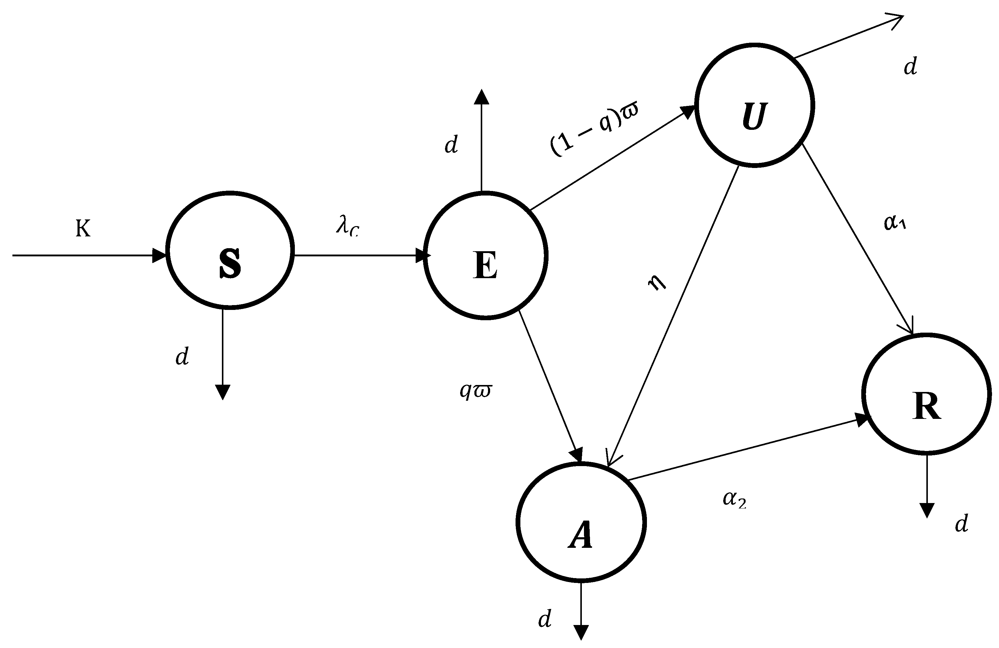
4. Theoretical Investigation of the Control Dynamics

Here, let us modify the corruption diffusion dynamical system (3) by considering three time-based control techniques. To express the control measures incorporated into the corruption diffusion dynamics in the community, we denoted the functions ${\mathrm{u}}_1\left(\mathrm{t}\right)$ as the protection control activity, ${\mathrm{u}}_2\left(\mathrm{t}\right)$ as the improvement activity, and ${\mathrm{u}}_3\left(\mathrm{t}\right)$ as the improvement activity, such that 0 $\le {\mathrm{u}}_1\left(\mathrm{t}\right)\le \mathrm{h},{\mathrm{u}}_2\left(\mathrm{t}\right)\le \mathrm{h}$ and ${\mathrm{u}}_3\left(\mathrm{t}\right)\le \mathrm{n}$ are the Lebesgue measurable controlling functions.

Measures to prevent corruption. The degree of the corruption prevention mechanism, or the efforts carried out to stop people from engaging in corrupt practices, is denoted by the control activity ${\mathrm{u}}_1\left(\mathrm{t}\right)$.

Corruption Improvement Techniques: The time-dependent control measures for unaware and aware corrupted persons are represented by ${\mathrm{u}}_2\left(\mathrm{t}\right)$ and ${\mathrm{u}}_3\left(\mathrm{t}\right)$, respectively.

The new optimal control dynamical system for the dynamical system (3) is reconstructed as:

$$\begin{array}{c}{}^{\mathrm{C}}D_t^{\phi }S={\mathsf{{\rm K}}}^{\phi }-\left((1-u_1\left(t\right)){\displaystyle \frac{{\mathsf{\beta }}^{\phi }({\rho }_1^{\phi }U+{\rho }_2^{\phi }A)}{N}}+d^{\phi }\right)S,\\ {}^{\mathrm{C}}D_t^{\phi }E=(1-u_1\left(t\right)){\displaystyle \frac{{\mathsf{\beta }}^{\phi }({\rho }_1^{\phi }U+{\rho }_2^{\phi }A)}{M}}-\left(d^{\phi }+{\varpi }^{\phi }\right)E,\\ {}^{\mathrm{C}}D_t^{\phi }U=(1-q^{\phi }){\varpi }^{\phi }E-(d^{\phi }+{\eta }^{\phi }+u_2(t){\alpha }_1^{\phi })U,\\ {}^{\mathrm{C}}D_t^{\phi }A=q^{\phi }{\varpi }^{\phi }E+{\eta }^{\phi }U-(d^{\phi }+u_3(t){\alpha }_2^{\phi })A,\\ {}^{\mathrm{C}}D_t^{\phi }R=u_2(t){\alpha }_1^{\phi }U+u_3(t){\alpha }_2^{\phi }A-d^{\phi }R,\end{array}$$

(14)

where $S\left(0\right)>0$, $E\left(0\right)\ge 0,U\left(0\right)\ge 0$, $A\left(0\right)\ge 0$, $R\left(0\right)\ge 0,$ and the set ${\mathsf{\Delta }}_C=\left\{{(u}_1,u_2,u_3):0u_1\left(t\right)\le 1,u_2\left(t\right)\le 1,u_3\left(t\right)\le 1,t\in \left[0,T_f\right]\right\}$, which contains control techniques where $T_f$ is the last moment to put control measures into action. The goal of constructing the control dynamical system is, at the expense of implementing control techniques, to raise the repentant people number and decrease the number of exposed people, unaware corrupted people, and aware corrupted people. In order to reduce the corrupted people, we construct the objective function denoted by

$$J\left(u_1, u_2,u_3\right)={\int }_0^{T_f}\left({\chi }_{1}E+{\chi }_2\mathrm{U}+{\chi }_3\mathrm{A}+{\displaystyle \frac{{\mathsf{\Gamma }}_1}{2}}{u}_1^2+{\displaystyle \frac{{\mathsf{\Gamma }}_2}{2}}{u}_2^2+{\displaystyle \frac{{\mathsf{\Gamma }}_3}{2}}{u}_3^2\right) dt.$$

(15)

System (15) minimizes ${ u}_1\left(t\right), u_2\left(t\right)$, and $u_3\left(t\right)$ in order to regulate the corrupted people number and the expense of applying protection and improvement control activities. The final time is represented by the constant $T_f$ in this section, the coefficients ${\chi }_1,{\chi }_2$ and ${\chi }_3$ are positive constants, and the costs relative to protection and improvement activities, ${\displaystyle \frac{{\mathsf{\Gamma }}_1}{2}}, {\displaystyle \frac{{\mathsf{\Gamma }}_2}{2}}$, and ${\displaystyle \frac{{\mathsf{\Gamma }}_3}{2}}$, correspond to the controls $u_1, u_2$, and $u_3$, respectively. Additionally, the units of integrand are balanced. The purpose is to minimize the objective function and determine the ideal values $U^{\ast }=\left(u_1^{\ast }, u_2^{\ast },u_3^{\ast }\right)$ of the controls $U=\left(u_1, u_2,u_3\right)$ so that the state trajectories $S^{\ast }, E^{\ast }, U^{\ast }, A^{\ast }, R^{\ast }$ are solutions of (15) in the specified time range $\left[0,T_f\right]$ with starting data. The cost associated with exposed individuals is denoted by the phrase “${\chi }_{1}E$” in the cost functional, the cost associated with moderately corrupted persons by the term “${\chi }_{2}U$”, and the cost associated with severely corrupted individuals by the term “${\chi }_3\mathrm{A}$”. Additionally, $T_f$ is the last time the control measures are applied, and ${\chi }_i$ and ${\mathsf{\Gamma }}_i$ are constants that are non-negative and indicate the cost for the triple control activities implementation and the related attempts to reduce the diffusion of corruption, respectively, for $i=\mathrm{1,2},3$.

Subject to the dynamical system represented by (14) with the given initial criteria, the goal of the corruption diffusion dynamical system (14) is to find the optimal value of the control activity $u(t)$ that minimizes the objective function described as $\underset{\overline{u} \in \overline{U}}{\min }J(\overline{u})$. The controlling vector is $\overline{u}=\{u_1, u_2, u_3)$, and the acceptable controls are the set $\overline{U}=\{\overline{u} \in {(L^{\infty }(\left[0,T_f\right]))}^3, 0 \le { u}_i \le 1, i=1, 2, 3\}$.

Existence and Suitability of Control Techniques: It is possible to rewrite the corruption diffusion dynamical system (3) with (4) as

$$D_t^{\phi }V=M\left(t,V\left(t\right)\right)+H\left(t,V\left(t\right)\right)\overline{u},0\mathrm{n}t\le T_f,V\left(t\right)=V_0,$$

where $V\left(t\right)=(S\left(t\right),E\left(t\right),U\left(t\right),A\left(t\right),R\left(t\right))$ symbolizes the variables, $u\left(t\right)=(u_1\left(t\right),u_2\left(t\right),u_3\left(t\right)$ represents control activities of the model (14), and

$$M\left(t,V\left(t\right)\right)=\left[\begin{array}{c}{\mathsf{{\rm K}}}^{\phi }-\left({\displaystyle \frac{{\mathsf{\beta }}^{\phi }\left({\rho }_1^{\phi }U+{\rho }_2^{\phi }A\right)}{N}}+d^{\phi }\right)S\\ {\displaystyle \frac{{\mathsf{\beta }}^{\phi }\left({\rho }_1^{\phi }U+{\rho }_2^{\phi }A\right)}{N}}S-\left(d^{\phi }+{\varpi }^{\phi }\right)E\\ {(1-q}^{\phi }){\varpi }^{\phi }E-\left(d^{\phi }+{\eta }^{\phi }\right)U\\ q^{\phi }{\varpi }^{\phi }E+{\mathsf{\eta }}^{\phi }U-{\mathrm{d}}^{\phi }A\\ -d^{\phi }R\end{array}\right],$$

$$H\left(t,V\left(t\right)\right)=\left[\begin{array}{ccc}{\displaystyle \frac{{\mathsf{\beta }}^{\phi }({\rho }_1^{\phi }U+{\rho }_2^{\phi }A)}{N}}\mathrm{S}& 0& 0\\ -{\displaystyle \frac{{\mathsf{\beta }}^{\phi }({\rho }_1^{\phi }U+{\rho }_2^{\phi }A)}{N}}\mathrm{S}& 0& 0\\ 0& -{\alpha }_1^{\phi }U& 0\\ 0& 0& -{\alpha }_2^{\phi }A\\ 0& {\alpha }_1^{\phi }U& {\alpha }_1^{\phi }U\end{array}\right].$$

Here, we must demonstrate the existence of the three ideal control techniques by proving the following conditions: the collection of control functions is a convex set, a bounded set, and a closed set, the control trajectories are non-empty, and $M\left(t,V\left(t\right)\right)+H\left(t,V\left(t\right)\right)$ is constrained by the control variables and state variables, and ${\chi }_{1}E+{\chi }_2\mathrm{U}+{\chi }_3\mathrm{A}+{\displaystyle \frac{{\mathsf{\Gamma }}_1}{2}}{u}_1^2+{\displaystyle \frac{{\mathsf{\Gamma }}_2}{2}}{u}_2^2+{\displaystyle \frac{{\mathsf{\Gamma }}_3}{2}}{u}_3^2$ on the collection $\overline{U}$ is convex.

Note that: The requirements listed below are predicated using definitions from the manuscript: as per the collection, the $\overline{U}$ definition is a convex set, a bounded set, and a closed set. Since $0d{u}_i\le 1,$ for $i=\mathrm{1,2},3$, the system dynamics (14) solutions are uniquely constrained based on similar criteria applied in the system dynamics (3). The solution $Y=(S,E,U,A,R)$ for the system dynamics (3) with the supplied initial population is non-empty with control functions values of${ u}_1=1,$ $u_2=0$, and ${ u}_3=0$ in the admissible control set $\overline{U}$ described above.

Theorem 6.

The function represented by $M\left(t,V\left(t\right)\right)+H\left(t,V\left(t\right)\right)\overline{u}$ meets at the corruption diffusion system dynamics solution $\overline{V}=(S,E,U,A,R)$ , where $‖M\left(t,\overline{V}\right)+H\left(t,\overline{V}\right)‖\le max(k_1,k_2)(‖\overline{V}‖+‖\overline{u}‖)$, $k_1=max(1+{\beta }^{\phi }\left({\rho }_1^{\phi }+{\rho }_2^{\phi }\right)+d^{\phi },d^{\phi }+{\varpi }^{\phi },d^{\phi }+{\eta }^{\phi }+{\alpha }_1^{\phi },d^{\phi }+{\alpha }_2^{\phi },d^{\phi })$, and $k_2=max({\beta }^{\phi }\left({\rho }_1^{\phi }+{\rho }_2^{\phi }\right), {\eta }^{\phi },1)$.

Proof. 

Let us describe $M\left(t,V\left(t\right)\right)$ as

$$M\left(t,V\left(t\right)\right)=\left[\begin{array}{ccccc}D& 0& 0& 0& 0\\ {\displaystyle \frac{{\mathsf{\beta }}^{\phi }({\rho }_1^{\phi }U+{\rho }_2^{\phi }A)}{N}}& -\left(d^{\phi }+{\varpi }^{\phi }\right)& 0& 0& 0\\ 0& {(1-q}^{\phi }){\varpi }^{\phi }& \left(d^{\phi }+{\eta }^{\phi }+{\alpha }_1^{\phi }\right)& 0& 0\\ 0& q^{\phi }{\varpi }^{\phi }& {\eta }^{\phi }& \left(d^{\phi }+{\alpha }_2^{\phi }\right)& 0\\ 0& 0& {\alpha }_1^{\phi }& {\alpha }_2^{\phi }& -d^{\phi }\end{array}\right]\left[\begin{array}{c}S\\ E\\ \mathrm{U}\\ \mathrm{A}\\ R\end{array}\right],$$

where $D={\displaystyle \frac{{\mathsf{{\rm K}}}^{\phi }}{S}}-{\displaystyle \frac{{\mathsf{\beta }}^{\phi }({\rho }_1^{\phi }U+{\rho }_2^{\phi }A)}{N}}$. Based on the conditions of the matrix $M\left(t,V\left(t\right)\right)$, we get ${\mathsf{{\rm K}}}^{\phi }\le S$ and, because we have demonstrated that the solution is bounded, $‖M\left(t,\overline{V}\right)‖\le \mathrm{m}\mathrm{a}\mathrm{x}(1+{\beta }^{\phi }\left({\rho }_1^{\phi }+{\rho }_2^{\phi }\right)+d^{\phi },d^{\phi }+{\varpi }^{\phi },d^{\phi }+{\eta }^{\phi }+{\alpha }_1^{\phi },d^{\phi }+{\alpha }_2^{\phi },d^{\phi })‖\overline{V}‖$. With the same approach, one can prove that $‖M\left(t,\overline{V}\right)‖\le \mathrm{m}\mathrm{a}\mathrm{x}({\beta }^{\phi }\left({\rho }_1^{\phi }+{\rho }_2^{\phi }\right), {\eta }^{\phi },1)‖\overline{u}‖$.□

Theorem 7.

We construct a function described by $Q\left(t,\overline{V},\overline{u}\right)={\chi }_{1}E+{\chi }_{2}U+{\chi }_{3}A+{\displaystyle \frac{{\Gamma }_1}{2}}{u}_1^2+{\displaystyle \frac{{\Gamma }_2}{2}}{u}_2^2+{\displaystyle \frac{{\Gamma }_3}{2}}{u}_3^2$ in the admissible control zone $\overline{U}$, which is convex, and k is a non-negative parameter that exists and that satisfies $Q\left(t,\overline{V},\overline{u}\right)\ge k\overline{u}$.

Proof. 

For function $Q\left(t,\overline{V},\overline{u}\right)$ one can obtain the matching matrix (Hessian), which is provided as

$$\mathbb{H}=\left[\begin{array}{ccc}2u_1& 0& 0\\ 0& 2u_2& 0\\ 0& 0& 2u_3\end{array}\right].$$

Consequently, $Q\left(t,\overline{V},\overline{u}\right)$ is strictly convex in $U$, since $H$ described above is a positive definite diagonal matrix in the area $\overline{U}$. Let $k=\mathrm{m}\mathrm{i}\mathrm{n}({\displaystyle \frac{{\mathsf{\Gamma }}_1}{2}},{\displaystyle \frac{{\mathsf{\Gamma }}_2}{2}},{\displaystyle \frac{{\mathsf{\Gamma }}_3}{2}})$, then $\mathbb{V}\left(t,\overline{Y},\overline{u}\right)={\chi }_{1}E+{\chi }_2\mathrm{U}+{\chi }_3\mathrm{A}+{\displaystyle \frac{{\mathsf{\Gamma }}_1}{2}}{u}_1^2+{\displaystyle \frac{{\mathsf{\Gamma }}_2}{2}}{u}_2^2+{\displaystyle \frac{{\mathsf{\Gamma }}_3}{2}}{u}_3^2\ge {\displaystyle \frac{{\mathsf{\Gamma }}_1}{2}}{u}_1^2+{\displaystyle \frac{{\mathsf{\Gamma }}_2}{2}}{u}_2^2+{\displaystyle \frac{{\mathsf{\Gamma }}_3}{2}}{u}_3^2\ge k({\displaystyle \frac{{\mathsf{\Gamma }}_1}{2}}{u}_1^2+{\displaystyle \frac{{\mathsf{\Gamma }}_2}{2}}{u}_2^2+{\displaystyle \frac{{\mathsf{\Gamma }}_3}{2}}{u}_3^2)$. Hence, we establish the required proof.□

Theorem 8.

The model-associated solutions ${\overline{Y}}^{\ast }=\left(S^{\ast },E^{\ast },U^{\ast },A^{\ast },R^{\ast }\right),$ as well as the optimal control point ${\overline{u}}^{\ast }=(u_1^{\ast },u_2^{\ast },u_3^{\ast })$ that minimize $J(\overline{u})$ on the collection $\overline{U}$ so that $\underset{\overline{u} \in \overline{U}}{\mathit{min}}J(\overline{u})=J({\overline{u}}^{\ast })$.

The requirement for optimality is, according to [17], the optimality necessary condition that the optimal control issues (14) and (15) must satisfy comes from Pontryagin’s Maximum Principle. Additionally, it is satisfied by transforming into a function (Hamiltonian function) that minimizes regard to the control activities $(u_1,u_2,u_3)$. The following is the derivation of the equivalent Hamiltonian for (14) and (15):

$$H\left(\overline{Y},\overline{u}, {\mathsf{{\rm K}}}^{\phi }\right)={\chi }_{1}E+{\chi }_2 \mathrm{U}+{\chi }_3 \mathrm{A}+{\displaystyle \frac{{\mathsf{\Gamma }}_1}{2}}{u}_1^2+{\displaystyle \frac{{\mathsf{\Gamma }}_2}{2}}{u}_2^2+{\displaystyle \frac{{\mathsf{\Gamma }}_3}{2}}{u}_3^2$$

$$\begin{array}{c}{\lambda }_1({\mathsf{{\rm K}}}^{\phi }-((1-u_1(t)){\displaystyle \frac{{\mathsf{\beta }}^{\phi }({\rho }_1^{\phi }U+{\rho }_2^{\phi }A)}{M}}+d^{\phi }\left)S\right)+{\lambda }_2\left(\begin{array}{c}(1-u_1(t)){\displaystyle \frac{{\mathsf{\beta }}^{\phi }({\rho }_1^{\phi }U+{\rho }_2^{\phi }A)}{N}}-\\ (d^{\phi }+{\varpi }^{\phi })E\end{array}\right)+\\ {\lambda }_3((1-q^{\phi }){\varpi }^{\phi }E-(d^{\phi }+{\eta }^{\phi }+u_2(t){\alpha }_1^{\phi })U)+{\lambda }_4(q^{\phi }{\varpi }^{\phi }E+{\eta }^{\phi }U-(d^{\phi }+d_2^{\phi }+u_3(t({\alpha }_2^{\phi })A)+{\lambda }_5(u_2(t){\alpha }_1^{\phi }U+\\ u_3\left(t\right){\alpha }_2^{\phi }A-d^{\phi }R),\end{array}$$

where the co-state or adjoint variables are ${\lambda }_1, {\lambda }_2, {\lambda }_3, {\lambda }_4,$ and ${\lambda }_5$ at time t.

Theorem 9.

Given solutions $u_i^{\ast }$ at $i=\mathrm{1,2},3$ and solutions of the system dynamics (14) that minimize the function illustrated in (15) in the region $\overline{U}$, there exist adjoints ${\lambda }_1(t), {\lambda }_2(t),{\lambda }_3(t),{\lambda }_4(t)$, and ${\lambda }_5(t)$ such that s:

$$\begin{array}{c}{}^{\mathrm{C}}D_t^{\phi }{\lambda }_1=\left({\lambda }_1-{\lambda }_2\right)\left(1-u_1\right){\displaystyle \frac{{\mathsf{\beta }}^{\phi }\left({\rho }_1^{\phi }U+{\rho }_2^{\phi }A\right)}{N}}\left(1-{\displaystyle \frac{S}{N}}\right)+d^{\phi }{\lambda }_1,\\ {}^{\mathrm{C}}D_t^{\phi }{\lambda }_2=({\lambda }_2-{\lambda }_1)(1-u_1)\frac{{\mathsf{\beta }}^{\phi }({\rho }_1^{\phi }U+{\rho }_2^{\phi }A)S}{N^2}+{\lambda }_2(d^{\phi }+{\varpi }^{\phi })-{\lambda }_3(1-q^{\phi }){\varpi }^{\phi }-{\lambda }_3{q}^{\phi }{\varpi }^{\phi }-{\chi }_1,\\ {}^{\mathrm{C}}D_t^{\phi }{\lambda }_3=\left({\lambda }_2-{\lambda }_1\right)\left(1-u_1\right)\left({\displaystyle \frac{{\mathsf{\beta }}^{\phi }\left({\rho }_1^{\phi }U+{\rho }_2^{\phi }A\right)S}{N^2}}-{\mathsf{\beta }}^{\phi }{\rho }_1^{\phi }{\displaystyle \frac{S}{N}}\right)+\left({\lambda }_3-{\lambda }_4\right){(\eta }^{\phi }+u_2)+{\lambda }_{3}B+{\lambda }_4{\alpha }_1^{\phi }-{\chi }_2,\\ {}^{\mathrm{C}}D_t^{\phi }{\lambda }_4=\left({\lambda }_2-{\lambda }_1\right)\left(1-u_1\right)\left({\displaystyle \frac{{\mathsf{\beta }}^{\phi }\left({\rho }_1^{\phi }U+{\rho }_2^{\phi }A\right)S}{N^2}}-{\mathsf{\beta }}^{\phi }{\rho }_2^{\phi }{\displaystyle \frac{S}{N}}\right)+\left({\lambda }_4-{\lambda }_5\right)({\alpha }_2^{\phi }+u_3)+{\lambda }_4\left(d^{\phi }+d_2^{\phi }\right)-{\chi }_3,\\ {}^{\mathrm{C}}D_t^{\phi }{\lambda }_5=\left({\lambda }_2-{\lambda }_1\right)\left(1-u_1\right){\displaystyle \frac{{\mathsf{\beta }}^{\phi }\left({\rho }_1^{\phi }U+{\rho }_2^{\phi }A\right)S}{M^2}}+{\lambda }_5{d}^{\phi },\end{array}$$

where $B=\left(d^{\phi }+{\alpha }_1^{\phi }\right).$ Then, for previously specified function H system’s transversality criteria, ${\mathsf{\lambda }}_{\mathrm{i}}^{\mathrm{*}}\left({\mathrm{T}}_{\mathrm{f}}\right)=0$ at $i=1, 2, \dots ,5,$ and the previously specified function H. Additionally, the best control parameters ($u_1^{\ast }$, $u_2^{\ast }$,$u_3^{\ast }$) that minimize $J\left(u_1, u_2,u_3\right)$ over $U$ are given by:

$$\begin{array}{c}{u}_1^{\ast }\left(t\right)=\max \left\{1, \mathrm{m}\mathrm{i}\mathrm{n}[0,{\displaystyle \frac{\left({\lambda }_1-{\lambda }_2\right)}{{\mathsf{\Gamma }}_1}}{\displaystyle \frac{{\mathsf{\beta }}^{\phi }\left({\rho }_1^{\phi }U+{\rho }_2^{\phi }A\right)S}{N}}]\right\},\\ u_2^{\ast }\left(t\right)=\max \left\{1, \mathrm{m}\mathrm{i}\mathrm{n}[0,{\displaystyle \frac{\left({\lambda }_3-{\lambda }_5\right)}{{\mathsf{\Gamma }}_2}}U]\right\},\\ u_3^{\ast }\left(t\right)=\max \left\{1, \mathrm{m}\mathrm{i}\mathrm{n}[0,{\displaystyle \frac{\left({\lambda }_4-{\lambda }_5\right)}{{\mathsf{\Gamma }}_3}}A]\right\},\end{array}$$

(16)

where ${\lambda }_1\left(t\right), {\lambda }_2\left(t\right), {\lambda }_3\left(t\right), {\lambda }_4\left(t\right), \mathrm{a}\mathrm{n}\mathrm{d} {\lambda }_5\left(t\right)$ adjoint variables, satisfying (14)–(16) with the following transversality conditions: ${\lambda }_1\left({\mathrm{T}}_{\mathrm{f}}\right)={\lambda }_2\left({\mathrm{T}}_{\mathrm{f}}\right),={\lambda }_3\left({\mathrm{T}}_{\mathrm{f}}\right)={\lambda }_4\left({\mathrm{T}}_{\mathrm{f}}\right)={\lambda }_5\left({\mathrm{T}}_{\mathrm{f}}\right)=0$ and

$$u_1^{\ast }=\left\{\begin{array}{c}0, if u_1\le 0,\\ u_1, if 0<u_1<1, \\ 1, if u_1>0,\end{array}\right.\mathrm{and} u_2^{\ast }=\left\{\begin{array}{c}0, if u_2\le 0,\\ u_2, if 0<u_2<1, \\ 1, if u_2>0.\end{array}\right.$$

Proof. 

Using similar approaches used in reference [19,36], applying the Pontryagins Maximum Principle, we can determine that the convexity of the integrand of $J$ with respect to controls ${ u}_1, u_2,$ and $u_3$, the boundedness of the state solutions, and the Lipschitz property of the state system with respect to the state variables all lead to the existence of an optimal solution with the corresponding optimal control result represented by:

^C$D_{{\mathrm{T}}_{\mathrm{f}}}^{\phi }{\lambda }_1={\displaystyle \frac{\partial H}{\partial S}}$, ^C$D_{{\mathrm{T}}_{\mathrm{f}}}^{\phi }{\lambda }_2={\displaystyle \frac{\partial H}{\partial E}}$, ^C$D_{{\mathrm{T}}_{\mathrm{f}}}^{\phi }{\lambda }_3={\displaystyle \frac{\partial H}{\partial U}}$, ^C$D_{{\mathrm{T}}_{\mathrm{f}}}^{\phi }{\lambda }_4={\displaystyle \frac{\partial H}{\partial A}}$ and ^C$D_{{\mathrm{T}}_{\mathrm{f}}}^{\phi }{\lambda }_5$ = ${\displaystyle \frac{\partial H}{\partial R}}$. Thus, the optimality conditions are obtained by differentiating the Hamiltonian function $H$ with respect to the control variables $u_1,u_2,$ and $u_3$: ${\displaystyle \frac{\partial H}{\partial u_1}}={\displaystyle \frac{\partial H}{\partial u_2}}={\displaystyle \frac{\partial H}{\partial u_3}}=0$. □

5. Results of Numerical Simulations

For quantitative validation of the theoretical investigation described in the previous sections, particularly the optimal control system dynamics (14), this study carried out simulations using numerical approaches by considering the values for the corruption diffusion system dynamics parameter values represented in

Table 2. Simulation-related parameters and values.

	Values	Source
$d$	0.0189	[36]
$\mathsf{{\rm K}}$	50.000	[19,21]
$\varpi$	0.2000	[37]
${\alpha }_1$	0.4500	[38]
$\eta$	0.4000	[38]
${\alpha }_2$	0.3800	[38]
$\mathsf{\beta }$	0.02340	[37]
$q$	0.5000	[39]
${\mathsf{\rho }}_1$	0.01	Assume
${\mathsf{\rho }}_2$	0.2	Assume

below.

Performing simulations for the corruption diffusion dynamics optimal control system (14) is fundamental to the vital pictorial view and verifies the qualitative (theoretical) investigation of the proposed dynamical system with optimal control strategies. Therefore, by modeling the execution of the potential strategy combinations of the suggested control measures, we report the simulation results of the study in this section. Considering Table 2 above, the optimal control system dynamics (14) were simulated using MATLAB 2016a and the usual Runge-Kutta numerical approach. Three scenarios, the application of single control activity, dual control activities, and triple control activities with assumed cost weight parameter values, were created from the potential combination strategies of the suggested control measures as ${\chi }_1={\chi }_2={\chi }_3=15$, ${\mathsf{\Gamma }}_1=38$, ${\mathsf{\Gamma }}_2=40$,${\mathsf{\Gamma }}_3=42$ and with various starting population numbers. We used the fractional order constant $\phi =0.82$ to numerically simulate the system dynamics variables in the optimum control system dynamics (14) for investigating the effects of the proposed control activities in the following three scenarios and possible methods in each of the scenarios.

Scenario A (Implement single control measure)

➢

Strategy 1: practicing the protection control measures, such as education, media awareness, etc. (i.e., $u_1\ne 0,{u_2=u}_3=0$).

Scenario B (Implement double control measures)

➢

Strategy 2: practicing the improvement control measures, such as education, fear of punishments, etc. ($u_1=0,{u_2\ne 0, u}_3\ne 0$) for unaware corrupted individuals.

Scenario C (Implement triple control measures)

➢

Strategy 3: practicing the protection control measures, such as education, media awareness, etc. Practicing the improvement control measures, such as education, fear of punishments, etc., for both unaware and aware corrupted people, which means $u_1\ne 0, u_2\ne 0$, and $u_3\ne 0$.

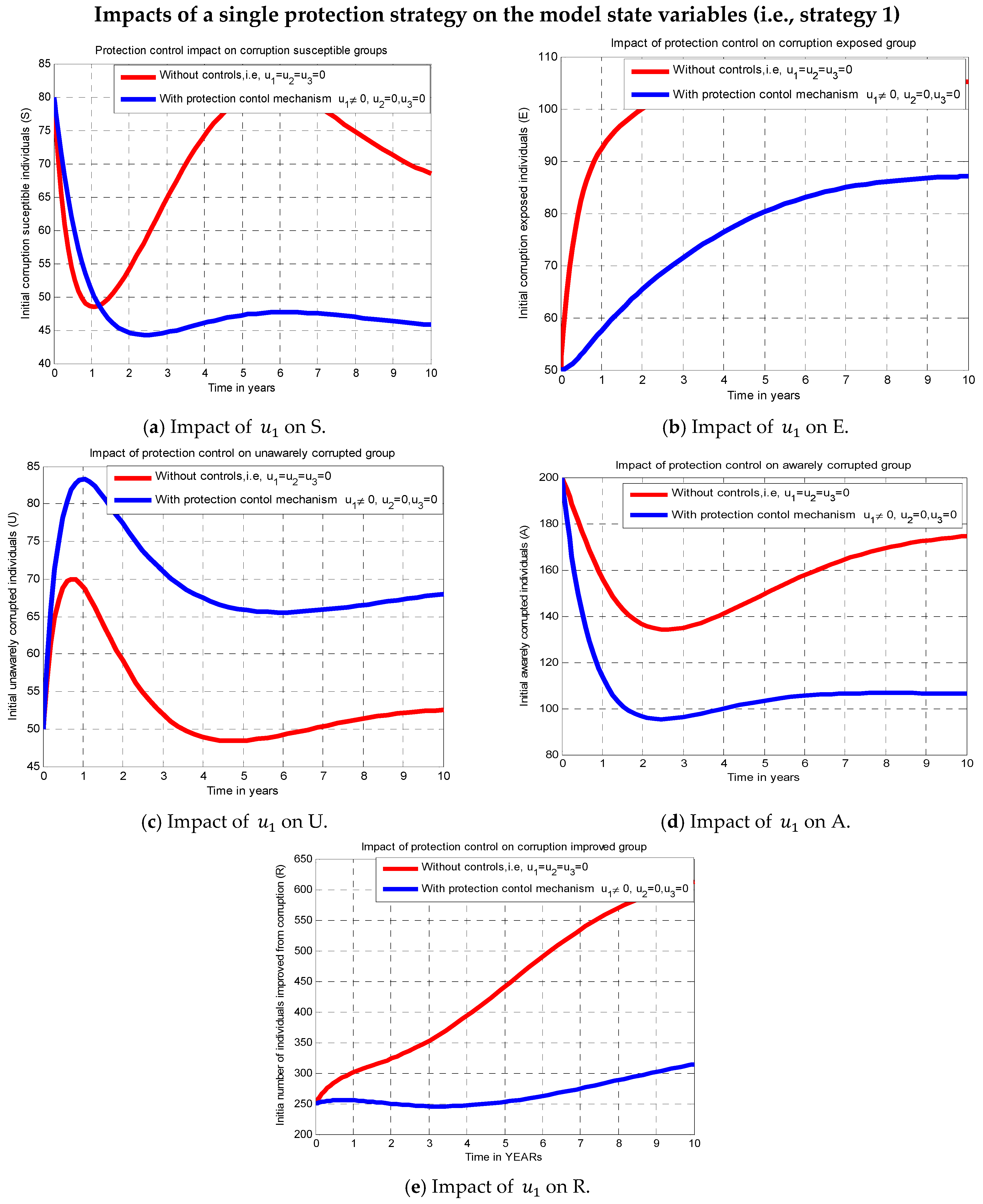
The effect of the strategy (i.e., $u_1\ne 0$,$u_2=0$, and $u_3=0$) known as the corruption prevention mechanism, by setting $\phi =0.75$, is examined in this subsection through numerical simulations where protection or improvement control strategies were not applied and when the corruption diffusion prevention strategy (strategy 1) was applied. Figure 2a–e each display a graphical interpretation that illustrates how the preventative method affects the dynamics of corruption diffusion. All susceptible, exposed, unaware corrupted, aware corrupted, and enhanced persons are drastically reduced when the protection control strategy $u_1$ is used, in contrast to the simulation scenario in which no control strategies were used.

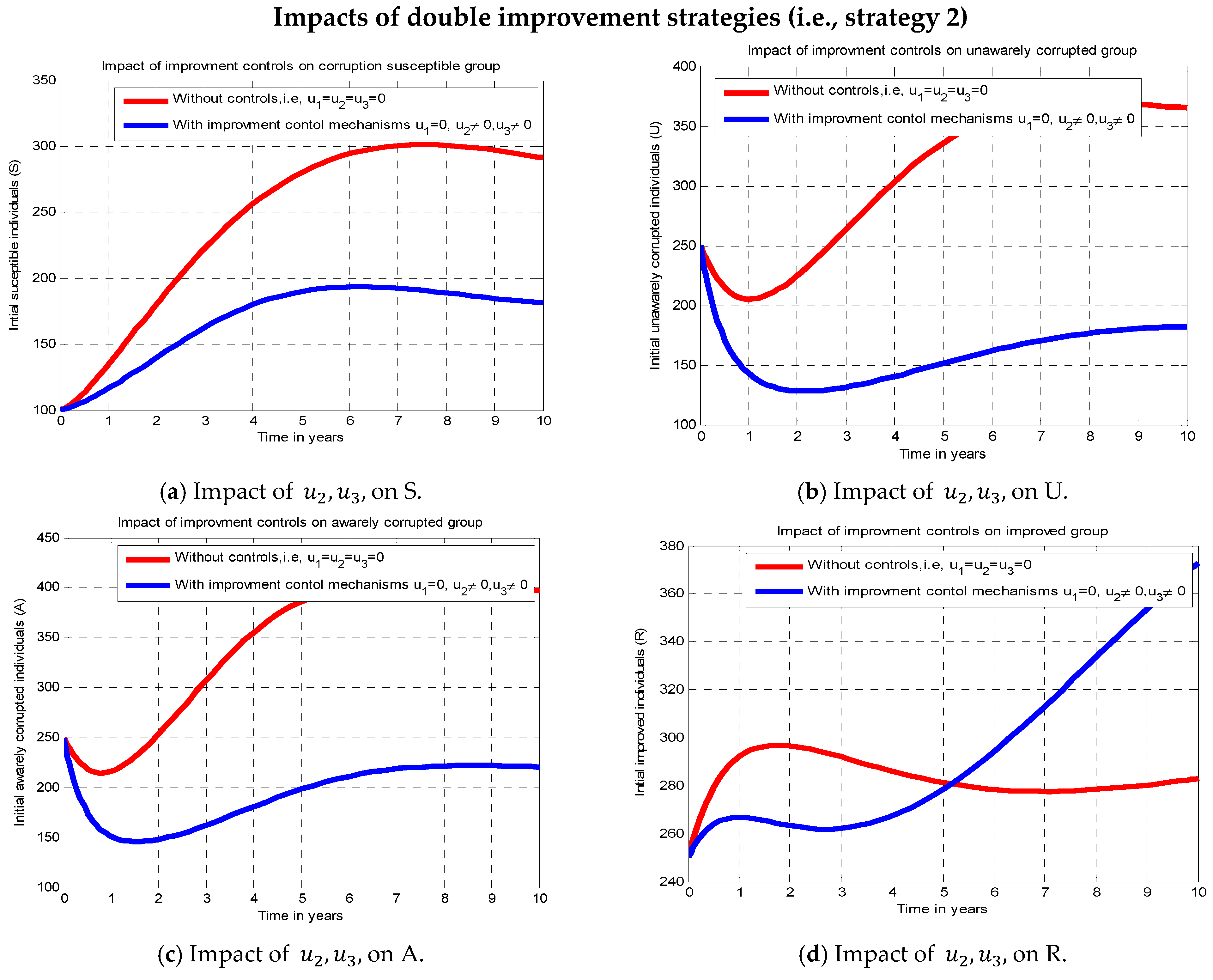
In this subsection, we conduct numerical simulations using the improvement strategies ${(u}_2\ne 0$ and $u_3\ne 0$, i.e., strategy 2), and without using the corruption protection control strategy ${(u}_1$). According to the simulation revealed in Figure 3 above, Figure 3a indicates that the number of people in the exposed class decreased somewhat in comparison to Figure 2b. Figure 3b,c confirm the effect of using double improvement strategies and show a rapid decline in comparison to the results in Figure 2c and Figure 2d, respectively. The impact of using double improvement control procedures is confirmed in Figure 3d, which also demonstrates that as improvement strategies rise, so does the number of people who are rescued from corrupted activities.

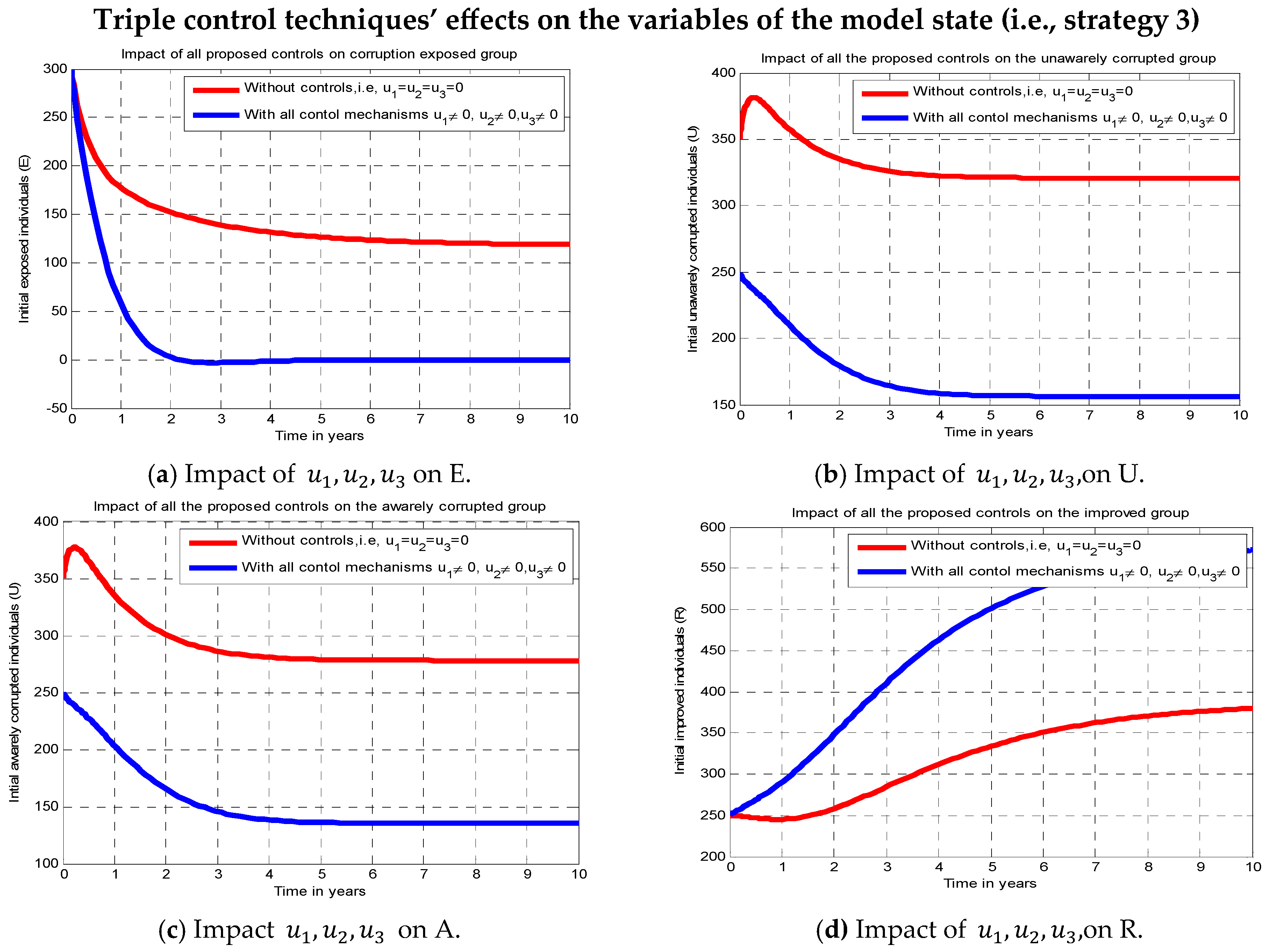
In this subsection, we conduct numerical simulations both with and without the implementation of all suggested regulating techniques $(u_1\ne 0 , u_2\ne 0,$ and $u_3\ne 0)$ (strategy 3) at the same time. We can examine the impacts of various control tactics on the system dynamic variables corruption status based on the results shown in Figure 4. All of the suggested controlling strategies have a significant result in reducing the exposed people by simulating without implementing all of the suggested control strategies, and by implementing any other control strategies, as shown in Figure 4a. Figure 4b illustrates the impact of putting all of the suggested controlling strategies into practice using the number of people who are unaware of corruption. This has a significant result in reducing people who are unaware and corrupted in comparison to the numbers shown in Figure 2c and Figure 3b, respectively. As compared to the corrupted people depicted in Figure 2d and Figure 3c, respectively, Figure 4c illustrates the impact of all suggested controlling strategies on the number of aware corrupted individuals and significantly reduces that number. In contrast to the number of repented persons depicted in Figure 2e and Figure 3d, respectively, Figure 4d illustrates the influence of all suggested control activities on the repented (improved) individuals and significantly increases repented people. Lastly, we can see from Figure 4 that, after ten years, corrupted people in the population significantly decline if all potential regulating activities $(u_1\ne 0, u_2\ne 0,$ and $u_3\ne 0,$ i.e., using strategy 3) are put into practice. Additionally, this approach is the most successful in reducing and controlling the dynamics of corruption dissemination in the population when compared to other approaches.

Figure 5 above reveals that whenever the fractional order constant decreases, the number of unaware and corrupted individuals decreases due to the memory effect of the fractional order derivative.

6. Investigation of Cost-Benefits

In order to compare and contrast possible control activities’ cost-benefits that are included in the fractional order optimum control problem (14), we conducted a cost-benefit investigation for the suggested control activities in this section. Applying the same standards as the study [9], which were established by $\mathrm{ICER}=\frac{\mathrm{Total} \mathrm{cost} \mathrm{Change} \mathrm{between} \mathrm{strategy} \mathrm{A} \mathrm{and} \mathrm{Strategy} \mathrm{B}}{\mathrm{Control} \mathrm{benefit} \mathrm{change} \mathrm{between} \mathrm{strategy} \mathrm{A} \mathrm{and} \mathrm{Strategy} \mathrm{B}}$, where the differences in the costs of corruption avoided, protected case costs, and improvement costs are among the factors included in the numerator of the incremental cost-benefit ratio, or ICER. On the other hand, the denominator of ICER takes into consideration the disparities in social outcomes, such as the aggregate number of corruption instances avoided. By placing the control activities in increasing order of benefit based on corrupted people avoided and leaving the condition with the biggest ICER value, the cost-benefits of various corruption diffusion control measures are assessed. Thus, each of the seven control strategies can be ranked in increasing order according to corrupted people avoided, as shown by

Table 3. Increasing the Order of Corruptions Averted for Strategies 1–3.

Strategy	Aggregate of Corruptions Averted	Aggregate Cost (in US$)	ICER Value
Strategy 1	4.0015 $\times {10}^5$	0.041 × ${10}^2$	$1.0250\times {10}^{-5}$
Strategy 3	4.0329 $\times {10}^5$	0.059 × ${10}^2$	$5.7325\times {10}^{-4}$
Strategy 2	4.1242 $\times {10}^5$	0.33 $\times {10}^2$	$2.9659\times {10}^{-3}$

, from the seven control strategies categorized by three scenarios, namely Scenario A, Scenario B, and Scenario C, respectively.

6.1. Investigation of Scenario A Cost-Effectiveness

To compare the two comparable strategies incrementally, the ICER is calculated for the control schemes Strategy 1 and Strategy 3 in Table 3. This is as follows:

$$\mathrm{ICER} (\mathrm{Strategy} 1)={\displaystyle \frac{0.041\times {10}^2}{4.0015\times {10}^5}}=1.0250\times {10}^{-5},$$

$$\mathrm{ICER} (\mathrm{Strategy} 3)={\displaystyle \frac{0.059\times {10}^2-0.041\times {10}^2}{4.0329\times {10}^5-4.0015\times {10}^5}}=5.7325\times {10}^{-4},$$

$$\mathrm{ICER} (\mathrm{Strategy} 2)={\displaystyle \frac{0.33\times {10}^2-0.059\times {10}^2}{4.1242\times {10}^5-4.0329\times {10}^5}}=2.9659\times {10}^{-3},$$

According to the analysis in Table 3, Strategy 3’s ICER value is higher than Strategy 1’s, indicating that it is less effective and more expensive than Strategy 1. The ICER for Strategy 1 and Strategy 2 was recalculated since we eliminated other competing strategies for scarce resources because Strategy 3 was too costly and ineffective.

We demonstrated that Strategy 2 should be eliminated since its ICER value was higher than Strategy 1 using comparable criteria and the findings shown in

Table 4. Strategy 1 and Strategy 2 comparison.

Strategy	Aggregate of Corruptions Averted	Aggregate Cost (in US$)	ICER
Strategy 1	4.0015 $\times {10}^5$	0.041 × ${10}^2$	$1.0250\times {10}^{-5}$
Strategy 2	4.1242 $\times {10}^5$	0.33 $\times {10}^2$	$2.3553\times {10}^{-3}$

. Therefore, we removed Strategy 2 from the lists provided in scenario A since it is more expensive than Strategy 1, as seen by the results in Table 4 above, and Strategy 1 has a higher potential cost-effectiveness.

6.2. Investigation of Scenario B Cost-Effectiveness

To compare the two comparison strategies, the ICER value is computed for the control activities (strategies), Strategy 6 and Strategy 4, as shown in

Table 5. For Strategies 4–6, the number of corruptions avoided increases in order.

Strategy	Aggregate of Corruptions Averted	Aggregate Cost (in US $)	ICER Value
Strategy 6	5.0015 $\times {10}^5$	0.064 × ${10}^2$	$1.2796\times {10}^{-5}$
Strategy 4	5.0329 $\times {10}^5$	0.071 × ${10}^2$	$2.2293\times {10}^{-4}$
Strategy 5	5.1242 $\times {10}^5$	0.43 $\times {10}^2$	$3.9407\times {10}^{-2}$

. This value is incrementally determined as follows:

$$\mathrm{ICER} (\mathrm{Strategy} 6)={\displaystyle \frac{0.064\times {10}^2}{5.0015\times {10}^5}}=1.2796\times {10}^{-5},$$

$$\mathrm{ICER} (\mathrm{Strategy} 4)={\displaystyle \frac{0.071\times {10}^2-0.064\times {10}^2}{5.0329\times {10}^5-5.0015\times {10}^5}}=2.2293\times {10}^{-4},$$

$$\mathrm{ICER} (\mathrm{Strategy} 5)={\displaystyle \frac{0.43\times {10}^2-0.071\times {10}^2}{5.1242\times {10}^5-5.0329\times {10}^5}}=3.9407\times {10}^{-2},$$

According to the cost analysis presented in Table 5, Strategy 6’s ICER value is greater than Strategy 4’s, indicating that Strategy 4 is less effective and more expensive than Strategy 6. The ICER for Strategy 6 and Strategy 5 was recalculated since we eliminated other competing strategies for scarce resources because Strategy 4 was too costly and ineffective.

We demonstrated that Strategy 5 should be eliminated since its ICER value was higher than Strategy 6 using comparable criteria and the findings shown in

Table 6. Strategy 6 and Strategy 5 comparison.

Strategy	Aggregate of Corruptions Averted	Aggregate Cost (in US $)	ICER
Strategy 6	5.0015 $\times {10}^5$	0.064 × ${10}^2$	$1.2796\times {10}^{-5}$
Strategy 5	5.1242 $\times {10}^5$	0.43 $\times {10}^2$	$2.9829\times {10}^{-3}$

. Therefore, we removed Strategy 5 from the lists provided in Scenario B since it is more cost-effective than Strategy 6, as demonstrated by the results in Table 5 above. Additionally, Strategy 6 has a high potential cost-effectiveness.

6.3. Investigation of Scenario C Cost-Effectiveness

We determined from

Table 7. Strategy 7.

Strategy	Aggregate of Corruptions Averted	Aggregate Cost (in US$)	ICER
Strategy 7	6.2341 $\times {10}^6$	1.5213 × ${10}^3$	$2.4402\times {10}^{-4}$

that method 7 is the most economical control method in Scenario C, as it is the only one shown in the above scenario. The combinations of collections of each of the control strategies with high potential cost-effectiveness from Scenarios A, B, and C, respectively, as mentioned above, are shown in the following

Table 8. Comparison of Strategies 1 and 6 for Control.

Strategy	Aggregate of Corruptions Averted	Aggregate Cost (in US$)	ICER
Strategy 1	4.0014 $\times {10}^5$	0.041 × ${10}^2$	$1.0250\times {10}^{-5}$
Strategy 6	5.0015 $\times {10}^5$	0.064 × ${10}^2$	2.3000 × ${10}^{-5}$
Strategy 7	6.2341 $\times {10}^6$	1.5213 × ${10}^3$	2.6520 × ${10}^{-3}$

below. This allows one to calculate the control strategy with the greatest potential in comparison to other potential strategies used to reduce and control the corruption diffusion problem in the population.

6.4. Cost-Effectiveness of the Collections

Based on the ICER values calculated in Table 8, we determined that Strategy 6 is more expensive than Strategy 1, as seen by the outcome displayed in Table 8 above. This suggests that Strategy 6 execution is less successful and more expensive than Strategy 1 implementation. The list of alternate control techniques vying for the same scarce resources is thus reduced to exclude Strategy 6. Finally, as seen in

Table 9. Compare Strategy 1 and Strategy 7 for Control.

Strategy	Aggregate of Corruptions Averted	Aggregate Cost (in US$)	ICER
Strategy 1	4.0014 $\times {10}^5$	0.041 × ${10}^2$	$1.0250\times {10}^{-5}$
Strategy 7	6.2341 $\times {10}^6$	1.5213 × ${10}^3$	6.6006 × ${10}^{-4}$

below, the ICER is recalculated for Strategies 1 and 7.

According to the results shown in Table 9, one can conclude that Strategy 7 is more expensive than Strategy 1 based on the ICER values calculated in that table. This suggests that Strategy 7 execution is less successful and more expensive than Strategy 1 implementation. The list of alternate control techniques vying for the same scarce resources is thus reduced to exclude Strategy 7. In the end, we determined that the most economical control strategy recommended to the stakeholders to lessen and manage the corruption diffusion issue in the population is Strategy 1, which involves implementing protection control measures like education, media awareness, etc. (i.e., $u_1\ne 0,{u_2=u}_3=0$).

7. Conclusions and Future Directions

In this study, the authors constructed and analyzed a fractional order model on the diffusion of corruption in the population with optimal control theory and also investigated the cost-benefit for the proposed control strategies. The theoretical part of this study analyzed the basic properties of the formulated model, such as the existence of the model solutions, the uniqueness of the model solutions, positivity, and the boundedness of the model solutions. This study calculated the model threshold number by using the matrix operator method and examined the stability of equilibrium points using the stability criterion for the fractional modeling approach and the model threshold number. This study also analyzed the corresponding fractional-order corruption diffusion control system dynamics with three time-dependent control measures using Pontryagin’s Maximum Principle. Furthermore, this study conducted a cost-benefit investigation for the controlling activities and numerically simulated the model using the parameter values stated in Table 2, the popular Runge-Kutta numerical fourth-order approach in MATLAB, in order to identify which of the three scenarios, such as implementing one control measure, two control measures, and three control measures, respectively. In this study, we have investigated the numerical simulation results of the optimal control problem by implementing each of the three control strategies (Strategy 1, Strategy 2, and Strategy 3) independently, and the results reveal that each of the strategies has a great impact on reducing and managing the corruption diffusion in the community. However, the cost-benefit analysis verified that Strategy 1, which did not incorporate punishment or fear of punishment, is the most cost-effective strategy as compared with the other two strategies. Therefore, the most cost-benefit control strategy recommended to the stakeholders to reduce and manage the corruption diffusion problem in the population is Strategy 1, which is implementing protection control measures like education and media awareness.

Finally, as the fractional order corruption diffusion model constructed in this study is not all-inclusive, potential researchers in the field can modify the model by adding more elements like the stochastic approach, individual age distribution, community roles, and sensitivity analysis, and since this study adopted parameter values from the literature carried out in different geographical locations, any interested researcher can validate the results of this study by collecting real corruption data from the community in the study area.

References

1. Teixeira, M.A.C.; Spinelli, M.V.C. Corruption: A Brief Review of Theoretical Approach. Beijing Law Rev. 2024, 15, 624–637. [Google Scholar] [CrossRef]
2. Kotola, B.S.; Teklu, S.W. A mathematical modeling analysis of racism and corruption codynamics with numerical simulation as infectious diseases. Comput. Math. Methods Med. 2022, 2022, 9977727. [Google Scholar]
3. Mokaya, N.O.; Alemmeh, H.T.; Ngari, C.G.; Muthuri, G.G. Mathematical modelling and analysis of corruption of morals amongst adolescents with control measures in Kenya. Discret. Dyn. Nat. Soc. 2021, 2021, 6662185. [Google Scholar]
4. Birhanu, Z.K.; Fantaye, A.K. Modeling and analysis of corruption dynamics incorporating media coverage. Commun. Math. Biol. Neurosci. 2022, 2022, 94. [Google Scholar]
5. Bonyah, E. Fractional optimal control for a corruption model. J. Prime Res. Math. 2020, 16, 11–29. [Google Scholar]
6. Graeff, P. Social mechanisms of corruption: Analytical sociology and its applicability to corruption research. Anal. Krit. 2016, 38, 53–72. [Google Scholar]
7. Tubanambazi, M.F.; Ruvuna, E. Modeling the Impacts of E-Government Services on Corruption Reduction in Rwanda: A Case Evidence From Nyamasheke District, Rwanda. Eur. J. Soc. Sci. Stud. 2021, 6, 1–24. [Google Scholar] [CrossRef]
8. Ghahari, S.; Queiroz, C.; Labi, S.; McNeil, S. Cluster forecasting of corruption using nonlinear autoregressive models with exogenous variables (NARX)—An artificial neural network analysis. Sustainability 2021, 13, 11366. [Google Scholar] [CrossRef]
9. Engida, H.A.; Gathungu, D.K.; Ferede, M.M.; Belay, M.A.; Kawe, P.C.; Mataru, B. Optimal control and cost-effectiveness analysis for the human melioidosis model. Heliyon 2024, 10, e26487. [Google Scholar]
10. Hassan, H. Social implications of corruption in developing countries: Case study of Pakistan and India. Cent. Eur. J. Public Policy 2022, 16, 1–13. [Google Scholar]
11. Wittberg, E. Corruption Risks in a Mature Democracy: Mechanisms of Social Advantage and Danger Zones for Corruption. Ph.D. Thesis, Linköping University Electronic Press, Linköping, Sweden, 2023. [Google Scholar]
12. Turkewitz, J.A.; Chemouni, B.H.; Mkrtchyan, A. Rwanda’s Anti-Corruption Experience: Actions, Accomplishments, and Lessons; World Bank Group: Washington, DC, USA, 2020. [Google Scholar]
13. Oyamada, E. Combating corruption in Rwanda: Lessons for policy makers. Asian Educ. Dev. Stud. 2017, 6, 249–262. [Google Scholar]
14. Roesli, M. Corruption Sociology. J. Soc. Political Sci. 2020, 1, 93–101. [Google Scholar]
15. Alemneh, H.T.; Alemu, N.Y. Mathematical modeling with optimal control analysis of social media addiction. Infect. Dis. Model. 2021, 6, 405–419. [Google Scholar]
16. Baba, B.A.; Bilgehan, B. Optimal control of a fractional order model for the COVID–19 pandemic. Chaos Solitons Fractals 2021, 144, 110678. [Google Scholar] [PubMed]
17. Islam, M.; Akbar, M.A. A study on the fractional-order COVID-19 SEIQR model and parameter analysis using homotopy perturbation method. Partial. Differ. Equ. Appl. Math. 2024, 12, 100960. [Google Scholar]
18. Ogunrinde, R.B.; Nwajeri, U.K.; Fadugba, S.E.; Ogunrinde, R.R.; Oshinubi, K.I. Dynamic model of COVID-19 and citizens reaction using fractional derivative. Alex. Eng. J. 2021, 60, 2001–2012. [Google Scholar]
19. Teklu, S.W. Analysis of fractional order model on higher institution students’ anxiety towards mathematics with optimal control theory. Sci. Rep. 2023, 13, 6867. [Google Scholar]
20. Gweryina, R.I.; Kura, M.Y.; Okwu, E. An epidemiological model of corruption with immunity clause in Nigeria. World J. Model. Simul. 2019, 15, 262–275. [Google Scholar]
21. Athithan, S.; Ghosh, M.; Li, X.-Z. Mathematical modeling and optimal control of corruption dynamics. Asian-Eur. J. Math. 2018, 11, 1850090. [Google Scholar]
22. Danford, O. Corruption Dynamics in Tanzania: Modeling the Effects of Control Strategies. Ph.D. Thesis, NM-AIST, Arusha, Tanzania, 2021. [Google Scholar]
23. Fantaye, A.K.; Birhanu, Z.K. Mathematical model and analysis of corruption dynamics with optimal control. J. Appl. Math. 2022, 2022, 8073877. [Google Scholar]
24. Alemneh, H.T. Mathematical modeling, analysis, and optimal control of corruption dynamics. J. Appl. Math. 2020, 2020, 5109841. [Google Scholar]
25. Tesfaye, A.W.; Alemneh, H.T. Analysis of a stochastic model of corruption transmission dynamics with temporary immunity. Heliyon 2023, 9, e12752. [Google Scholar]
26. Balatif, O.; Boujallal, L.; Labzai, A.; Rachik, M. Stability analysis of a fractional-order model for abstinence behavior of registration on the electoral lists. Int. J. Differ. Equ. 2020, 2020, 4325640. [Google Scholar]
27. Mandal, M.; Jana, S.; Nandi, S.K.; Kar, T.K. Modelling and control of a fractional-order epidemic model with fear effect. Energy Ecol. Environ. 2020, 5, 421–432. [Google Scholar] [CrossRef] [PubMed]
28. Mekonnen, T.T. Mathematical model analysis and numerical simulation for codynamics of meningitis and pneumonia infection with intervention. Sci. Rep. 2022, 12, 2639. [Google Scholar]
29. Pontryagin, L.S.; Boltyanskii, V.; Gamkrelidze, R.; Mishchenko, E.; Trirogoff, K.; Neustadt, L.; Pontryagin, L.S. Selected Works: The Mathematical Theory of Optimal Processes; Routledge: London, UK, 2018. [Google Scholar]
30. Rezapour, S.; Etemad, S.; Mohammadi, H. A mathematical analysis of a system of Caputo–Fabrizio fractional differential equations for the anthrax disease model in animals. Adv. Differ. Equ. 2020, 2020, 481. [Google Scholar]
31. Baleanu, D.; Mohammadi, H.; Rezapour, S. Analysis of the model of HIV-1 infection of CD 4+ T-cell with a new approach of fractional derivative. Adv. Differ. Equ. 2020, 2020, 71. [Google Scholar]
32. Rezapour, S.; Mohammadi, H.; Samei, M.E. SEIR epidemic model for COVID-19 transmission by Caputo derivative of fractional order. Adv. Differ. Equ. 2020, 2020, 490. [Google Scholar]
33. Van den Driessche, P.; Watmough, J. Reproduction numbers and sub-threshold endemic equilibria for compartmental models of disease transmission. Math. Biosci. 2002, 180, 29–48. [Google Scholar] [CrossRef] [PubMed]
34. Vargas-De-León, C. Volterra-type Lyapunov functions for fractional-order epidemic systems. Commun. Nonlinear Sci. Numer. Simul. 2015, 24, 75–85. [Google Scholar] [CrossRef]
35. Sadki, M.; Harroudi, S.; Allali, K. Fractional-order SIR epidemic model with treatment cure rate. Partial. Differ. Equ. Appl. Math. 2023, 8, 100593. [Google Scholar]
36. Teklu, S.W.; Kotola, B.S.; Alemneh, H.T. Smoking and alcoholism dual addiction dissemination model analysis with optimal control theory and cost-effectiveness. PLoS ONE 2024, 19, e0309356. [Google Scholar]
37. Yang, Q.; Chen, D.; Zhao, T.; Chen, Y. Fractional calculus in image processing: A review. Fract. Calc. Appl. Anal. 2016, 19, 1222–1249. [Google Scholar]
38. Yousef, A.M.; Salman, S.M. Backward bifurcation in a fractional-order SIRS epidemic model with a nonlinear incidence rate. Int. J. Nonlinear Sci. Numer. Simul. 2016, 17, 401–412. [Google Scholar]
39. Petráš, I. Fractional-Order Nonlinear Systems: Modeling, Analysis and Simulation; Springer Science & Business Media: Berlin/Heidelberg, Germany, 2011. [Google Scholar]
Figure 1. The schematic diagram where λ C is described in Equation (8).
Fractalfract 09 00207 g001
Figure 2. Impact of u 1 on the status of corrupted people with φ = 0.75 .
Fractalfract 09 00207 g002
Figure 3. How the corruption statuses of various population groups are affected by the corruption improvement strategies ( u 2   and   u 3 ) with φ = 0.75 .
Fractalfract 09 00207 g003
Figure 4. Effects of Strategy 3 on the level of corruption in various demographic groups with φ = 0.75 .
Fractalfract 09 00207 g004
Figure 5. Effects of fractional orders on unaware and corrupted individuals variable U , whenever φ = 0.5 ,   φ = 0.75 , and φ = 1 .
Fractalfract 09 00207 g005