Investigation of Delay-Induced Hopf Bifurcation in a Fractional Neutral-Type Neural Network

Abstract

This paper investigates stability switches induced by Hopf bifurcation in a fractional three-neuron network that incorporates both neutral time delay and communication delay, as well as a general structure. Initially, we simplified the characteristic equation by eliminating trigonometric terms associated with purely imaginary roots, enabling us to derive the Hopf bifurcation conditions for communication delay while treating the neutral time delay as a constant. The results reveal that communication delay can drive a stable equilibrium into instability once it exceeds the Hopf bifurcation threshold. Furthermore, we performed a sensitivity analysis to identify the fractional order and neutral delay as the two most sensitive parameters influencing the bifurcation value for the illustrative example. Notably, in contrast to neural networks with only retarded delays, our numerical observations show that the Hopf bifurcation curve is non-monotonic, highlighting that the neural network with a fixed communication delay can exhibit stability switches and eventually stabilize as the neutral delay increases.

1. Introduction

Neural networks, as energetic frontal interdisciplinary studies, have garnered considerable scientific interest due to their applications as diverse as pattern recognition and deep learning in recent decades [1,2]. These applications are closely contingent on the related dynamical mechanism of the designed neural networks. Therefore, we need to detail the dynamics of neural networks [3]. In scenarios where neural networks are designed to address practical issues, communication delays cannot be avoided due to the influence of the reaction to the speed of electronic devices or the non-instantaneous propagation of signals of biological neurons [4,5]. Moreover, the incorporation of communication delays in neural networks is essential and can be better used to describe some circuits [6]. However, communication delays usually have adverse effects on the stability performance of neural networks, which may give rise to stability switches due to Hopf bifurcation. This transition of stability could be pertinent to some cognitive diseases [7]. The study of Hopf bifurcation in neural networks still constitutes a important topic that deserves further study [8,9].

On the other hand, when large-scale integrated circuits constitute a neural network, the appearance of various categories of time delays is undeniable [10,11,12]. For example, the rate of change of the state variables pertaining to some neural networks hinges on the current and past states, as well as the change in past rates [13,14,15]. That is, time delays appear not only in the current states themselves but also in the time derivative of past states of the neurons. This kind of neural networks is called a neutral-type neural network [16,17]. The dynamics of a neutral-type neural network without external input can be characterized by the following system, as introduced in [18]:

$$\begin{array}{cc}\hfill {\displaystyle \frac{\mathrm{d}{x}_i\left(t\right)}{\mathrm{d}t}}=& -k_i{x}_i\left(t\right)+\sum _{j=1}^n{\alpha }_{ij}{f}_j\left(x_j\left(t\right)\right)+\sum _{j=1}^n{\beta }_{ij}{f}_j\left(x_j(t-{\tau }_x)\right)\hfill \\ & +\sum _{j=1}^n{d}_{ij}{x}_j(t-{\tau }_y),i=1,2,\cdots ,n.\hfill \end{array}$$

(1)

In system (1), $x_i\left(t\right)$ relates to the state variable of the i-th neuron at time t; $k_i>0$ represents the internal decay rate; $f(·)$ stands for the neuron activation function; ${\alpha }_{ij}$, ${\beta }_{ij}$, and $d_{ij}$ refer to the connection weight, the delayed connection weight and the neutral delayed connection, respectively, of the three neurons; ${\tau }_x\mathrm{and}{\tau }_y$ measure the constant communication delay and the constant neutral time delay, respectively. They presented the equilibrium global stability criteria. Since neutral-type neural networks can precisely characterize the complicated properties of neural cells, including neuron reactions [19,20], they have attracted many investigations in recent years [21,22].

Recently, fractional differential equations have gained increasing recognition for their effectiveness in modeling the temporal evolution of neural networks, thanks to the unique strengths of fractional calculus [23,24,25]. These advantages include its ability to capture memory effects, provide better parameter fitting, and describe the behavior of the inverse power law [26,27]. As a result, fractional differential equations have garnered significant attention in the study of neural networks, with numerous works exploring their applications in this context [28,29]. For instance, research has demonstrated that the drift effects observed in fingerprints related to Fracmemristors can only be accurately described using fractional-order systems [30]. Additionally, it has been revealed that neuronal responses inherently follow the principles of fractional derivatives [28], further underscoring the relevance of fractional calculus in neural network modeling. Consequently, fractional neural networks have emerged as a promising advancement in the field [31,32]. There are now numerous definitions of fractional derivatives, each suited to different application scenarios [33]. Among the classical definitions are the Caputo, Grünwald–Letnikov, and Riemann–Liouville derivatives. Compared to the other two classical fractional derivatives, the Caputo derivative of a constant function and its initial conditions are the same as those of the integer-order derivative. In addition, the Caputo derivative is a special case of the unified fractional derivative defined in [34]. Therefore, many researchers utilize the Caputo derivative to describe the memory properties of neurons, benefiting from its intuitive physical interpretation and wide applicability across diverse fields [35]. For instance, the authors in [36,37] incorporate the Caputo derivative into neutral-type neural networks, examining their robust stability and asymptotic stability, respectively.

Most previous studies have primarily focused on stability analysis, with relatively little attention given to Hopf bifurcation induced by two delays in neutral-type neural networks. While recent research has increasingly explored Hopf bifurcation in fractional neural networks with retarded delays [24,25], investigations into more complex scenarios—such as fractional neural networks that incorporate both neutral and retarded delays, as well as networks with more than two neurons—remain limited [38,39]. This gap underscores the need for further exploration in this direction. To address this limitation, our study systematically examined the impact of both neutral and retarded delays on the Hopf bifurcation dynamics of fractional neural networks. Specifically, we incorporated the Caputo derivative into system (1) following the approach in [36] and considered the case where $n=3$. As a result, the dynamics of our fractional neutral-type neural network can be described by the following system:

$$\left\{\begin{array}{cc}\hfill D^{\vartheta }{x}_1\left(t\right)=& -k_1{x}_1\left(t\right)+{\alpha }_{11}f\left(x_1\left(t\right)\right)+{\alpha }_{12}f\left(x_2\left(t\right)\right)+{\alpha }_{13}f\left(x_3\left(t\right)\right)\hfill \\ & +{\beta }_{11}f\left(x_1(t-{\tau }_x)\right)+{\beta }_{12}f\left(x_2(t-{\tau }_x)\right)+{\beta }_{13}f\left(x_3(t-{\tau }_x)\right)\hfill \\ & +d_{11}{D}^{\vartheta }{x}_1(t-{\tau }_y)+d_{12}{D}^{\vartheta }{x}_2(t-{\tau }_y)+d_{13}{D}^{\vartheta }{x}_3(t-{\tau }_y),\hfill \\ \hfill D^{\vartheta }{x}_2\left(t\right)=& -k_2{x}_2\left(t\right)+{\alpha }_{21}f\left(x_1\left(t\right)\right)+{\alpha }_{22}f\left(x_2\left(t\right)\right)+{\alpha }_{23}f\left(x_3\left(t\right)\right)\hfill \\ & +{\beta }_{21}f\left(x_1(t-{\tau }_x)\right)+{\beta }_{22}f\left(x_2(t-{\tau }_x)\right)+{\beta }_{23}f\left(x_3(t-{\tau }_x)\right)\hfill \\ & +d_{21}{D}^{\vartheta }{x}_1(t-{\tau }_y)+d_{22}{D}^{\vartheta }{x}_2(t-{\tau }_y)+d_{23}{D}^{\vartheta }{x}_3(t-{\tau }_y),\hfill \\ \hfill D^{\vartheta }{x}_3\left(t\right)=& -k_3{x}_2\left(t\right)+{\alpha }_{31}f\left(x_1\left(t\right)\right)+{\alpha }_{32}f\left(x_2\left(t\right)\right)+{\alpha }_{33}f\left(x_3\left(t\right)\right)\hfill \\ & +{\beta }_{31}f\left(x_1(t-{\tau }_x)\right)+{\beta }_{32}f\left(x_2(t-{\tau }_x)\right)+{\beta }_{33}f\left(x_3(t-{\tau }_x)\right)\hfill \\ & +d_{31}{D}^{\vartheta }{x}_1(t-{\tau }_y)+d_{32}{D}^{\vartheta }{x}_2(t-{\tau }_y)+d_{33}{D}^{\vartheta }{x}_3(t-{\tau }_y).\hfill \end{array}\right.$$

(2)

In system (2), the symbol $D^{\vartheta }g\left(t\right)$$(\vartheta \in (0,1\left]\right)$ refers to the Caputo fractional derivative of fractional order $\vartheta$ for a function $g\left(t\right),t\in [0,+\infty )$; the initial conditions are

$$x_i\left(t\right)={\Psi }_i\left(t\right),t\in [-\max \{{\tau }_x,{\tau }_y\},0],i=1,2,3,$$

where ${\Psi }_i\left(t\right)\in C([-\max \{{\tau }_x,{\tau }_y\},0],\mathbb{R})$. We usually assume that Hypothesis 1 $f(·)\in C^1(\mathbb{R},\mathbb{R})$, $f\left(0\right)=0$ and $f^{\prime }\left(0\right)\ne 0$. Obviously, Hypothesis 1 implies the origin is the equilibrium of system (2). We intend to, as best as we are able, procure the conditions for the Hopf bifurcation induced by delays for system (2).

Building on the previous discussions, we analyze the instability behaviors due to Hopf bifurcation of system (2). The main contributions and novelties of this paper are as follows:

• System (2) extends the works of Gupta [9] and Li et al. [40] by incorporating neutral terms, while also generalizing the systems studied by Huang et al. [41] and Kumar et al. [39] by considering a network with more than two neurons and a more generalized structure.
• We establish the conditions under which system (2) can undergo bifurcation without imposing additional parameter constraints. Notably, our analysis does not require assumptions such as identical neurons [9] or the equality of communication delay and neutral time delay [42].
• Our numerical findings indicate that neutral delay and fractional order are the two most sensitive parameters affecting the bifurcation value. Notably, neutral delay can trigger multiple stability switches.

In summary, our results could provide a new avenue to understand the dynamics of neural networks. The rest of this paper is structured as follows. In Section 2, by eliminating all trigonometric functions of the characteristic equation with purely imaginary roots, we establish criteria to detect the Hopf bifurcation point of communication delay. It is shown that the system can not preserve its stability when the communication delay increases through the Hopf bifurcation point. In Section 3, we provide a numerical example to verify the validation of the technique used. We finalize our paper with some conclusions in Section 4.

2. Main Results

In this section, we present the main results of this paper. The proof of our results is structured as follows. First, we derive the associated characteristic Equation (4) using the Laplace transform. Next, we establish the conditions for the local stability of the trivial equilibrium of system (2) in the absence of delays. We then determine the neutral delay range within which the system (2) remains stable. Finally, we provide the conditions for the occurrence of Hopf bifurcation induced by communication delay, considering the neutral time delay within its stability interval.

We linearize system (2) at origin yielding

$$\left\{\begin{array}{cc}\hfill D^{\vartheta }{x}_1\left(t\right)=& -k_1{x}_1\left(t\right)+a_{11}{x}_1\left(t\right)+a_{12}{x}_2\left(t\right)+a_{13}{x}_3\left(t\right)\hfill \\ & +b_{11}{x}_1(t-{\tau }_x)+b_{12}{x}_2(t-{\tau }_x)+b_{13}{x}_3(t-{\tau }_x)\hfill \\ & +d_{11}{D}^{\vartheta }{x}_1(t-{\tau }_y)+d_{12}{D}^{\vartheta }{x}_2(t-{\tau }_y)+d_{13}{D}^{\vartheta }{x}_3(t-{\tau }_y),\hfill \\ \hfill D^{\vartheta }{x}_2\left(t\right)=& -k_2{x}_2\left(t\right)+a_{21}{x}_1\left(t\right)+a_{22}{x}_2\left(t\right)+a_{23}{x}_3\left(t\right)\hfill \\ & +b_{21}{x}_1(t-{\tau }_x)+b_{22}{x}_2(t-{\tau }_x)+b_{23}{x}_3(t-{\tau }_x)\hfill \\ & +d_{21}{D}^{\vartheta }{x}_1(t-{\tau }_y)+d_{22}{D}^{\vartheta }{x}_2(t-{\tau }_y)+d_{23}{D}^{\vartheta }{x}_3(t-{\tau }_y),\hfill \\ \hfill D^{\vartheta }{x}_3\left(t\right)=& -k_3{x}_2\left(t\right)+a_{31}{x}_1\left(t\right)+a_{32}{x}_2\left(t\right)+a_{33}{x}_3\left(t\right)\hfill \\ & +b_{31}{x}_1(t-{\tau }_x)+b_{32}{x}_2(t-{\tau }_x)+b_{33}{x}_3(t-{\tau }_x)\hfill \\ & +d_{31}{D}^{\vartheta }{x}_1(t-{\tau }_y)+d_{32}{D}^{\vartheta }{x}_2(t-{\tau }_y)+d_{33}{D}^{\vartheta }{x}_3(t-{\tau }_y),\hfill \end{array}\right.$$

(3)

where $a_{ij}={\alpha }_{ij}{f}^{\prime }\left(0\right)$ and $b_{ij}={\beta }_{ij}{f}^{\prime }\left(0\right)$.

Inspired by the ideas in [43,44], we can procure the following characteristic determinant for system (3) by performing Laplace transform on both sides of (3):

$$\begin{array}{cc}\hfill & \left|\begin{array}{cc}{s}^{\vartheta }+k_1-a_{11}-b_{11}{\mathrm{e}}^{-s{\tau }_x}-d_{11}{s}^{\vartheta }{\mathrm{e}}^{-s{\tau }_y}& -a_{12}-b_{12}{\mathrm{e}}^{-s{\tau }_x}-d_{12}{s}^{\vartheta }{\mathrm{e}}^{-s{\tau }_y}\\ -a_{21}-b_{21}{\mathrm{e}}^{-s{\tau }_x}-d_{21}{s}^{\vartheta }{\mathrm{e}}^{-s{\tau }_y}& s^{\vartheta }+k_2-a_{22}-b_{22}{\mathrm{e}}^{-s{\tau }_x}-d_{22}{s}^{\vartheta }{\mathrm{e}}^{-s{\tau }_y}\\ -a_{31}-b_{31}{\mathrm{e}}^{-s{\tau }_x}-d_{31}{s}^{\vartheta }{\mathrm{e}}^{-s{\tau }_y}& -a_{32}-b_{32}{\mathrm{e}}^{-s{\tau }_x}-d_{32}{s}^{\vartheta }{\mathrm{e}}^{-s{\tau }_y}\end{array}\right.\\ \hfill & \left.\begin{array}{c}-a_{13}-b_{13}{\mathrm{e}}^{-s{\tau }_x}-d_{13}{s}^{\vartheta }{\mathrm{e}}^{-s{\tau }_y}\\ -a_{23}-b_{23}{\mathrm{e}}^{-s{\tau }_x}-d_{23}{s}^{\vartheta }{\mathrm{e}}^{-s{\tau }_y}\\ s^{\vartheta }+k_3-a_{33}-b_{33}{\mathrm{e}}^{-s{\tau }_x}-d_{33}{s}^{\vartheta }{\mathrm{e}}^{-s{\tau }_y}\end{array}\right|=0.\end{array}$$

That is,

$$\begin{array}{cc}\hfill & {\varphi }_3\left(s\right){\mathrm{e}}^{-3s{\tau }_x}+({\varphi }_2\left(s\right)-{\psi }_2\left(s\right){\mathrm{e}}^{-s{\tau }_y}){\mathrm{e}}^{-2s{\tau }_x}+{\varphi }_0\left(s\right)+{\psi }_{01}\left(s\right){\mathrm{e}}^{-s{\tau }_y}\hfill \\ \hfill +& \left({\varphi }_1\left(s\right)+{\psi }_{11}\left(s\right){\mathrm{e}}^{-s{\tau }_y}-{\psi }_{12}\left(s\right){\mathrm{e}}^{-2s{\tau }_y}\right){\mathrm{e}}^{-s{\tau }_x}+{\psi }_{02}\left(s\right){\mathrm{e}}^{-2s{\tau }_y}-{\psi }_{03}\left(s\right){\mathrm{e}}^{-3s{\tau }_y}=0,\hfill \end{array}$$

(4)

where

$$\begin{array}{cc}\hfill {\varphi }_3\left(s\right)=& c_{30},\hfill \\ \hfill {\varphi }_2\left(s\right)=& c_{21}{s}^{\vartheta }+c_{20},\hfill \\ \hfill {\psi }_2\left(s\right)=& l_{21}{s}^{\vartheta },\hfill \\ \hfill {\varphi }_1\left(s\right)=& c_{12}{s}^{2\vartheta }+c_{11}{s}^{\vartheta }+c_{10},\hfill \\ \hfill {\psi }_{11}\left(s\right)=& l_{12}{s}^{2\vartheta }+l_{11}{s}^{\vartheta },\hfill \\ \hfill {\psi }_{12}\left(s\right)=& l_{13}{s}^{2\vartheta },\hfill \\ \hfill {\varphi }_0\left(s\right)=& c_{03}{s}^{3\vartheta }+c_{02}{s}^{2\vartheta }+c_{01}{s}^{\vartheta }+c_{00},\hfill \\ \hfill {\psi }_{01}\left(s\right)=& q_{13}{s}^{3\vartheta }+q_{12}{s}^{2\vartheta }+q_{11}{s}^{\vartheta },\hfill \\ \hfill {\psi }_{02}\left(s\right)=& q_{23}{s}^{3\vartheta }+q_{22}{s}^{2\vartheta },\hfill \\ \hfill {\psi }_{03}\left(s\right)=& q_{33}{s}^{3\vartheta },\hfill \end{array}$$

and

$$\begin{array}{cc}\hfill c_{30}=& b_{11}(b_{23}{b}_{32}-b_{22}{b}_{33})+b_{12}{b}_{21}{b}_{33}-b_{12}{b}_{23}{b}_{31}-b_{13}{b}_{21}{b}_{32}+b_{13}{b}_{22}{b}_{31},\hfill \\ \hfill c_{21}=& b_{11}(b_{33}+b_{22})+b_{22}{b}_{33}-b_{12}{b}_{21}-b_{13}{b}_{31}-b_{23}{b}_{32},\hfill \\ \hfill c_{20}=& a_{11}(b_{23}{b}_{32}-b_{22}{b}_{33})+a_{22}(b_{13}{b}_{31}-b_{11}{b}_{33})+a_{33}(b_{12}{b}_{21}-b_{11}{b}_{22})\hfill \\ \hfill & +b_{11}(a_{23}{b}_{32}+a_{32}{b}_{23}+b_{22}{k}_3+b_{33}{k}_2)+b_{22}(a_{13}{b}_{31}+a_{31}{b}_{13}+b_{33}{k}_1)\hfill \\ \hfill & -a_{23}{b}_{12}{b}_{31}-a_{31}{b}_{12}{b}_{23}-a_{32}{b}_{13}{b}_{21}-b_{12}{b}_{21}{k}_3-b_{13}{b}_{31}{k}_2-a_{12}{b}_{23}{b}_{31}\hfill \\ \hfill & +b_{33}(a_{12}{b}_{21}+a_{21}{b}_{12})-a_{13}{b}_{21}{b}_{32}-a_{21}{b}_{13}{b}_{32}-b_{23}{b}_{32}{k}_1,\hfill \\ \hfill l_{21}=& b_{11}(b_{22}{d}_{33}+b_{33}{d}_{22}-b_{23}{d}_{32}-b_{32}{d}_{23})+b_{22}(b_{33}{d}_{11}-b_{13}{d}_{31}-b_{31}{d}_{13})\hfill \\ \hfill & -b_{33}(b_{12}{d}_{21}+b_{21}{d}_{12})-b_{23}{b}_{32}{d}_{11}-b_{13}{b}_{31}{d}_{22}-b_{12}{b}_{21}{d}_{33}+b_{21}{b}_{32}{d}_{13}\hfill \\ \hfill & +b_{13}(b_{21}{d}_{32}+b_{32}{d}_{21})+b_{12}(b_{23}{d}_{31}+b_{31}{d}_{23})+b_{23}{b}_{31}{d}_{12},\hfill \\ \hfill c_{12}=& -b_{11}-b_{22}-b_{33},\hfill \\ \hfill c_{11}=& a_{11}(b_{33}+b_{22})+a_{22}(b_{11}+b_{33})+a_{33}(b_{11}+b_{22})-b_{11}(k_3+k_2)-b_{22}(k_1+k_3)\hfill \\ \hfill & -b_{33}(k_1+k_2)-a_{13}{b}_{31}-a_{21}{b}_{12}-a_{23}{b}_{32}-a_{31}{b}_{13}-a_{32}{b}_{23}-a_{12}{b}_{21},\hfill \\ \hfill c_{10}=& a_{11}(a_{23}{b}_{32}+a_{32}{b}_{23}+b_{22}{k}_3+b_{33}{k}_2-a_{22}{b}_{33}-a_{33}{b}_{22})-k_2(a_{13}{b}_{31}+a_{31}{b}_{13})\hfill \\ \hfill & +a_{22}(a_{13}{b}_{31}+a_{31}{b}_{13}+b_{11}{k}_3+b_{33}{k}_1-a_{33}{b}_{11})\hfill \\ \hfill & +a_{33}(a_{12}{b}_{21}+a_{21}{b}_{12}+b_{11}{k}_2+b_{22}{k}_1)-k_1(a_{23}{b}_{32}+a_{32}{b}_{23})\hfill \\ \hfill & +b_{11}(a_{23}{a}_{32}-k_2{k}_3)+b_{22}(a_{13}{a}_{31}-k_1{k}_3)+b_{33}(a_{12}{a}_{21}-k_1{k}_2)\hfill \\ \hfill & -k_3(a_{12}{b}_{21}+a_{21}{b}_{12})-a_{12}(a_{23}{b}_{31}+a_{31}{b}_{23})-a_{13}(a_{21}{b}_{32}+a_{32}{b}_{21})\hfill \\ \hfill & -a_{21}{a}_{32}{b}_{13}-a_{23}{a}_{31}{b}_{12},\hfill \\ \hfill l_{12}=& b_{11}(d_{22}+d_{33})+b_{22}(d_{11}+d_{33})+b_{33}(d_{11}+d_{22})-d_{21}{b}_{12}-d_{31}{b}_{13}-d_{12}{b}_{21}\hfill \\ \hfill & -b_{23}{d}_{32}-d_{13}{b}_{31}-b_{32}{d}_{23},\hfill \\ \hfill l_{11}=& -a_{11}(b_{22}{d}_{33}+b_{33}{d}_{22}-b_{23}{d}_{32}-b_{32}{d}_{23})\hfill \\ \hfill & -a_{22}(b_{11}{d}_{33}+b_{33}{d}_{11}-b_{13}{d}_{31}-b_{31}{d}_{13})\hfill \\ \hfill & -a_{33}(b_{11}{d}_{22}+b_{22}{d}_{11}-b_{12}{d}_{21}-b_{21}{d}_{12})\hfill \\ \hfill & +b_{11}(a_{23}{d}_{32}+a_{32}{d}_{23}+d_{22}{k}_3+d_{33}{k}_2)\hfill \\ \hfill & +b_{22}(a_{13}{d}_{31}+a_{31}{d}_{13}+d_{11}{k}_3+d_{33}{k}_1)\hfill \\ \hfill & +b_{33}(a_{12}{d}_{21}+a_{21}{d}_{12}+d_{11}{k}_2+d_{22}{k}_1)\hfill \\ \hfill & +d_{11}(a_{23}{b}_{32}+a_{32}{b}_{23})+d_{22}(a_{13}{b}_{31}+a_{31}{b}_{13})+d_{33}(a_{12}{b}_{21}+a_{21}{b}_{12})\hfill \\ \hfill & -k_1(b_{23}{d}_{32}+b_{32}{d}_{23})-k_2(b_{13}{d}_{31}+b_{31}{d}_{13})-k_3(b_{12}{d}_{21}+b_{21}{d}_{12})\hfill \\ \hfill & -a_{12}(b_{23}{d}_{31}+b_{31}{d}_{23})-a_{13}(b_{21}{d}_{32}+b_{32}{d}_{21})-a_{21}(b_{13}{d}_{32}+b_{32}{d}_{13})\hfill \\ \hfill & -a_{23}(b_{12}{d}_{31}+b_{31}{d}_{12})-a_{31}(b_{12}{d}_{23}+b_{23}{d}_{12})-a_{32}(b_{13}{d}_{21}+b_{21}{d}_{13}),\hfill \\ \hfill l_{13}=& b_{11}(d_{22}{d}_{33}-d_{23}{d}_{32})+b_{22}(d_{11}{d}_{33}-d_{13}{d}_{31})+b_{33}(d_{11}{d}_{22}-d_{12}{d}_{21})\hfill \\ \hfill & -d_{11}(b_{23}{d}_{32}+b_{32}{d}_{23})-d_{22}(b_{13}{d}_{31}+b_{31}{d}_{13})-d_{33}(b_{12}{d}_{21}+b_{21}{d}_{12})\hfill \\ \hfill & +b_{12}{d}_{23}{d}_{31}+b_{13}{d}_{21}{d}_{32}+b_{21}{d}_{13}{d}_{32}+b_{23}{d}_{12}{d}_{31}+b_{31}{d}_{12}{d}_{23}+b_{32}{d}_{13}{d}_{21},\hfill \\ \hfill c_{03}=& 1,\hfill \\ \hfill c_{02}=& k_1+k_2+k_3-a_{11}-a_{22}-a_{33},\hfill \\ \hfill c_{01}=& a_{11}(a_{22}+a_{33}-k_2-k_3)+a_{22}(a_{33}-k_1-k_3)-a_{33}(k_1+k_2)+k_1(k_2+k_3)\hfill \\ \hfill & -a_{13}{a}_{31}-a_{12}{a}_{21}-a_{23}{a}_{32}+k_2{k}_3,\hfill \\ \hfill c_{00}=& a_{11}\left(a_{22}(k_3-a_{33})+a_{23}{a}_{32}+k_2{a}_{33}-k_2{k}_3\right)+a_{22}(a_{13}{a}_{31}+a_{33}{k}_1-k_1{k}_3)\hfill \\ \hfill & +a_{33}(a_{12}{a}_{21}-k_1{k}_2)+k_1(k_2{k}_3-a_{23}{a}_{32})-a_{13}{a}_{21}{a}_{32}-a_{13}{a}_{31}{k}_2\hfill \\ \hfill & -a_{12}{a}_{21}{k}_3-a_{12}{a}_{23}{a}_{31},\hfill \\ \hfill q_{13}=& -(d_{22}+d_{11}+d_{33}),\hfill \\ \hfill q_{12}=& a_{11}(d_{22}+d_{33})+a_{22}(d_{11}+d_{33})+a_{33}(d_{11}+d_{22})-d_{11}(k_3+k_2)-d_{22}(k_1+k_3)\hfill \\ \hfill & -d_{33}(k_1+k_2)-a_{13}{d}_{31}-a_{21}{d}_{12}-a_{23}{d}_{32}-a_{31}{d}_{13}-a_{32}{d}_{23}-a_{12}{d}_{21},\hfill \\ \hfill q_{11}=& -(a_{11}(a_{22}{d}_{33}+a_{33}{d}_{22}-a_{23}{d}_{32}-a_{32}{d}_{23}-d_{22}{k}_3-d_{33}{k}_2)+a_{21}{a}_{32}{d}_{13}\hfill \\ \hfill & +a_{12}(a_{23}{d}_{31}+a_{31}{d}_{23})+a_{22}(a_{33}{d}_{11}-a_{13}{d}_{31}-a_{31}{d}_{13}-d_{11}{k}_3-d_{33}{k}_1)\hfill \\ \hfill & -a_{33}(a_{12}{d}_{21}+a_{21}{d}_{12}+d_{11}{k}_2+d_{22}{k}_1)+d_{11}(k_2{k}_3-a_{23}{a}_{32})\hfill \\ \hfill & +d_{22}(k_1{k}_3-a_{13}{a}_{31})+d_{33}(k_1{k}_2-a_{12}{a}_{21})+k_1(a_{23}{d}_{32}+a_{32}{d}_{23})\hfill \\ \hfill & +k_2(a_{13}{d}_{31}+a_{31}{d}_{13})+k_3(a_{12}{d}_{21}+a_{21}{d}_{12})\hfill \\ \hfill & +a_{13}(a_{21}{d}_{32}+a_{32}{d}_{21})+a_{23}{a}_{31}{d}_{12}),\hfill \\ \hfill q_{23}=& d_{11}(d_{22}+d_{33})+d_{22}{d}_{33}-d_{12}{d}_{21}-d_{13}{d}_{31}-d_{23}{d}_{32},\hfill \\ \hfill q_{22}=& a_{11}(d_{23}{d}_{32}-d_{22}{d}_{33})+a_{22}(d_{13}{d}_{31}-d_{11}{d}_{33})+a_{33}(d_{12}{d}_{21}-d_{11}{d}_{22})\hfill \\ \hfill & +d_{33}(a_{12}{d}_{21}+a_{21}{d}_{12})+d_{11}(a_{23}{d}_{32}+a_{32}{d}_{23}+d_{22}{k}_3+d_{33}{k}_2)\hfill \\ \hfill & +d_{22}(a_{13}{d}_{31}+a_{31}{d}_{13}+d_{33}{k}_1)-a_{13}{d}_{21}{d}_{32}-a_{21}{d}_{13}{d}_{32}-a_{23}{d}_{12}{d}_{31}\hfill \\ \hfill & -a_{31}{d}_{12}{d}_{23}-a_{32}{d}_{13}{d}_{21}-d_{12}{d}_{21}{k}_3-d_{13}{d}_{31}{k}_2-a_{12}{d}_{23}{d}_{31}-d_{23}{d}_{32}{k}_1,\hfill \\ \hfill q_{33}=& d_{11}(d_{22}{d}_{33}-d_{23}{d}_{32})+d_{12}{d}_{23}{d}_{31}+d_{13}{d}_{21}{d}_{32}-d_{12}{d}_{21}{d}_{33}-d_{13}{d}_{31}{d}_{22}.\hfill \end{array}$$

We first consider the scenario ${\tau }_x={\tau }_y=0$; we then convert Equation (4) into

$$\begin{array}{c}\hfill s^{3\vartheta }+{\iota }_1{s}^{2\vartheta }+{\iota }_2{s}^{\vartheta }+{\iota }_3=0,\end{array}$$

(5)

where

$$\begin{array}{cc}\hfill {\iota }_1=& {\displaystyle \frac{c_{02}+c_{12}+l_{12}+q_{12}+q_{22}-l_{13}}{c_{03}+q_{13}+q_{23}-q_{33}}},\hfill \\ \hfill {\iota }_2=& {\displaystyle \frac{c_{01}+c_{11}+c_{21}+l_{11}+q_{11}-l_{21}}{c_{03}+q_{13}+q_{23}-q_{33}}},\hfill \\ \hfill {\iota }_3=& {\displaystyle \frac{c_{00}+c_{10}+c_{20}+c_{30}}{c_{03}+q_{13}+q_{23}-q_{33}}}.\hfill \end{array}$$

In the remainder of this paper, we assume the following.

Hypothesis 2.

${\iota }_{\zeta }>0(\zeta =1,2,3),{\iota }_1{\iota }_2-{\iota }_3>0.$

We can deduce that all the roots of Equation (5) are in the left-half complex plane by dint of the results set forth in [43]. Therefore, the following result is true.

Lemma 1. 

The origin of system (2) is stable provided ${\tau }_x={\tau }_y=0$.

Now, we explore the scenario when communication delay is absent. Then, Equation (4) turns into

$$\begin{array}{cc}\hfill & {\varphi }_0\left(s\right)+{\varphi }_1\left(s\right)+{\varphi }_2\left(s\right)+{\varphi }_3\left(s\right)+\left({\psi }_{01}\left(s\right)+{\psi }_{11}\left(s\right)-{\psi }_2\left(s\right)\right){\mathrm{e}}^{-s{\tau }_y}\hfill \\ \hfill +& \left({\psi }_{02}\left(s\right)-{\psi }_{12}\left(s\right)\right){\mathrm{e}}^{-2s{\tau }_y}-{\psi }_{03}\left(s\right){\mathrm{e}}^{-3s{\tau }_y}=0.\hfill \end{array}$$

(6)

Multiplying ${\mathrm{e}}^{2s{\tau }_y}$ on both sides of Equation (6), we have

$$\begin{array}{cc}\hfill & -{\psi }_{03}\left(s\right){\mathrm{e}}^{-s{\tau }_y}+{\psi }_{02}\left(s\right)-{\psi }_{12}\left(s\right)+\left({\psi }_{01}\left(s\right)+{\psi }_{11}\left(s\right)-{\psi }_2\left(s\right)\right){\mathrm{e}}^{s{\tau }_y}\hfill \\ \hfill +& \left({\varphi }_0\left(s\right)+{\varphi }_1\left(s\right)+{\varphi }_2\left(s\right)+{\varphi }_3\left(s\right)\right){\mathrm{e}}^{2s{\tau }_y}=0.\hfill \end{array}$$

(7)

Suppose $s=\varsigma {\mathrm{e}}^{i{\displaystyle \frac{\pi }{2}}}(\varsigma >0)$ is a root of Equation (7). Performing some algebra yields

$$\left\{\begin{array}{c}{\displaystyle {\mathfrak{R}}_3\cos 2\varsigma {\tau }_y-{\mathfrak{T}}_3\sin 2\varsigma {\tau }_y+({\mathfrak{R}}_2+{\mathfrak{R}}_0)\cos \varsigma {\tau }_y+({\mathfrak{T}}_0-{\mathfrak{T}}_2)\sin \varsigma {\tau }_y+{\mathfrak{R}}_1=0,}\hfill \\ {\displaystyle {\mathfrak{T}}_3\cos 2\varsigma {\tau }_y+{\mathfrak{R}}_3\sin 2\varsigma {\tau }_y+({\mathfrak{T}}_2+{\mathfrak{T}}_0)\cos \varsigma {\tau }_y+({\mathfrak{R}}_2-{\mathfrak{R}}_0)\sin \varsigma {\tau }_y+{\mathfrak{T}}_1=0,}\hfill \end{array}\right.$$

(8)

where

$$\begin{array}{cc}\hfill {\mathfrak{R}}_0=& -q_{33}{\varsigma }^{3\vartheta }\cos \left({\displaystyle \frac{3\vartheta \pi }{2}}\right),\hfill \\ \hfill {\mathfrak{T}}_0=& -q_{33}{\varsigma }^{3\vartheta }\sin \left({\displaystyle \frac{3\vartheta \pi }{2}}\right),\hfill \\ \hfill {\mathfrak{R}}_1=& q_{23}{\varsigma }^{3\vartheta }\cos \left({\displaystyle \frac{3\vartheta \pi }{2}}\right)+q_{22}{\varsigma }^{2\vartheta }\cos \left({\displaystyle \frac{2\vartheta \pi }{2}}\right)-l_{13}{\varsigma }^{2\vartheta }\cos \left({\displaystyle \frac{2\vartheta \pi }{2}}\right),\hfill \\ \hfill {\mathfrak{T}}_1=& q_{23}{\varsigma }^{3\vartheta }\sin \left({\displaystyle \frac{3\vartheta \pi }{2}}\right)+q_{22}{\varsigma }^{2\vartheta }\sin \left({\displaystyle \frac{2\vartheta \pi }{2}}\right)-l_{13}{\varsigma }^{2\vartheta }\sin \left({\displaystyle \frac{2\vartheta \pi }{2}}\right),\hfill \\ \hfill {\mathfrak{R}}_2=& q_{13}{\varsigma }^{3\vartheta }\cos \left({\displaystyle \frac{3\vartheta \pi }{2}}\right)+q_{12}{\varsigma }^{2\vartheta }\cos \left({\displaystyle \frac{2\vartheta \pi }{2}}\right)+q_{11}{\varsigma }^{\vartheta }\cos \left({\displaystyle \frac{\vartheta \pi }{2}}\right)\hfill \\ \hfill & +l_{12}{\varsigma }^{2\vartheta }\cos \left({\displaystyle \frac{2\vartheta \pi }{2}}\right)+l_{11}{\varsigma }^{\vartheta }\cos \left({\displaystyle \frac{\vartheta \pi }{2}}\right)-l_{21}{\varsigma }^{\vartheta }\cos \left({\displaystyle \frac{\vartheta \pi }{2}}\right),\hfill \\ \hfill {\mathfrak{T}}_2=& q_{13}{\varsigma }^{3\vartheta }\sin \left({\displaystyle \frac{3\vartheta \pi }{2}}\right)+q_{12}{\varsigma }^{2\vartheta }\sin \left({\displaystyle \frac{2\vartheta \pi }{2}}\right)+q_{11}{\varsigma }^{\vartheta }\sin \left({\displaystyle \frac{\vartheta \pi }{2}}\right)\hfill \\ \hfill & +l_{12}{\varsigma }^{2\vartheta }\sin \left({\displaystyle \frac{2\vartheta \pi }{2}}\right)+l_{11}{\varsigma }^{\vartheta }\sin \left({\displaystyle \frac{\vartheta \pi }{2}}\right)-l_{21}{\varsigma }^{\vartheta }\sin \left({\displaystyle \frac{\vartheta \pi }{2}}\right),\hfill \\ \hfill {\mathfrak{R}}_3=& c_{03}{\varsigma }^{3\vartheta }\cos \left({\displaystyle \frac{3\vartheta \pi }{2}}\right)+c_{02}{\varsigma }^{2\vartheta }\cos \left({\displaystyle \frac{2\vartheta \pi }{2}}\right)+c_{01}{\varsigma }^{\vartheta }\cos \left({\displaystyle \frac{\vartheta \pi }{2}}\right)+c_{00}+c_{10}+c_{20}+c_{30}\hfill \\ \hfill & +c_{12}{\varsigma }^{2\vartheta }\cos \left({\displaystyle \frac{2\vartheta \pi }{2}}\right)+c_{11}{\varsigma }^{\vartheta }\cos \left({\displaystyle \frac{\vartheta \pi }{2}}\right)+c_{21}{\varsigma }^{\vartheta }\cos \left({\displaystyle \frac{\vartheta \pi }{2}}\right),\hfill \\ \hfill {\mathfrak{T}}_3=& c_{03}{\varsigma }^{3\vartheta }\sin \left({\displaystyle \frac{3\vartheta \pi }{2}}\right)+c_{02}{\varsigma }^{2\vartheta }\sin \left({\displaystyle \frac{2\vartheta \pi }{2}}\right)+c_{01}{\varsigma }^{\vartheta }\sin \left({\displaystyle \frac{\vartheta \pi }{2}}\right)\hfill \\ \hfill & +c_{12}{\varsigma }^{2\vartheta }\sin \left({\displaystyle \frac{2\vartheta \pi }{2}}\right)+c_{11}{\varsigma }^{\vartheta }\sin \left({\displaystyle \frac{\vartheta \pi }{2}}\right)+c_{21}{\varsigma }^{\vartheta }\sin \left({\displaystyle \frac{\vartheta \pi }{2}}\right).\hfill \end{array}$$

On the other hand, multiplying ${\mathrm{e}}^{s{\tau }_y}$ on both sides of Equation (6) yields

$$\begin{array}{cc}\hfill & -{\psi }_{03}\left(s\right){\mathrm{e}}^{-2s{\tau }_y}+\left({\psi }_{02}\left(s\right)-{\psi }_{12}\left(s\right)\right){\mathrm{e}}^{-s{\tau }_y}+\left({\psi }_{01}\left(s\right)+{\psi }_{11}\left(s\right)-{\psi }_2\left(s\right)\right)\hfill \\ \hfill +& \left({\varphi }_0\left(s\right)+{\varphi }_1\left(s\right)+{\varphi }_2\left(s\right)+{\varphi }_3\left(s\right)\right){\mathrm{e}}^{s{\tau }_y}=0.\hfill \end{array}$$

(9)

We can deduce the following equations by substituting $s=\varsigma {\mathrm{e}}^{i{\displaystyle \frac{\pi }{2}}}(\varsigma >0)$ into Equation (9):

$$\left\{\begin{array}{c}{\displaystyle {\mathfrak{R}}_0\cos 2\varsigma {\tau }_y+{\mathfrak{T}}_0\sin 2\varsigma {\tau }_y+({\mathfrak{R}}_1+{\mathfrak{R}}_3)\cos \varsigma {\tau }_y+({\mathfrak{T}}_1-{\mathfrak{T}}_3)\sin \varsigma {\tau }_y+{\mathfrak{R}}_2=0,}\hfill \\ {\displaystyle {\mathfrak{T}}_0\cos 2\varsigma {\tau }_y-{\mathfrak{R}}_0\sin 2\varsigma {\tau }_y+({\mathfrak{T}}_1+{\mathfrak{T}}_3)\cos \varsigma {\tau }_y+({\mathfrak{R}}_3-{\mathfrak{R}}_1)\sin \varsigma {\tau }_y+{\mathfrak{T}}_2=0.}\hfill \end{array}\right.$$

(10)

We can solve $\cos 2\varsigma {\tau }_y,\sin 2\varsigma {\tau }_y$ from Equation (10):

$$\left\{\begin{array}{c}{\displaystyle \cos 2\varsigma {\tau }_y=\frac{\left({\mathfrak{R}}_0({\mathfrak{R}}_1+{\mathfrak{R}}_3)+{\mathfrak{T}}_0({\mathfrak{T}}_1+{\mathfrak{T}}_3)\right)\cos \varsigma {\tau }_y+\left({\mathfrak{R}}_0({\mathfrak{T}}_1-{\mathfrak{T}}_3)+{\mathfrak{T}}_0({\mathfrak{R}}_3-{\mathfrak{R}}_1)\right)\sin \varsigma {\tau }_y+{\mathfrak{R}}_0{\mathfrak{R}}_2+{\mathfrak{T}}_0{\mathfrak{T}}_2}{-({\mathfrak{R}}_0^2+{\mathfrak{T}}_0^2)},}\hfill \\ {\displaystyle \sin 2\varsigma {\tau }_y=\frac{\left({\mathfrak{T}}_0({\mathfrak{R}}_1+{\mathfrak{R}}_3)-{\mathfrak{R}}_0({\mathfrak{T}}_1+{\mathfrak{T}}_3)\right)\cos \varsigma {\tau }_y+\left({\mathfrak{R}}_0({\mathfrak{R}}_1-{\mathfrak{R}}_3)+{\mathfrak{T}}_0({\mathfrak{T}}_1-{\mathfrak{T}}_3)\right)\sin \varsigma {\tau }_y-{\mathfrak{R}}_0{\mathfrak{T}}_2+{\mathfrak{R}}_2{\mathfrak{T}}_0}{-({\mathfrak{R}}_0^2+{\mathfrak{T}}_0^2)}.}\hfill \end{array}\right.$$

Substituting these into Equation (8) results in

$$\left\{\begin{array}{c}{\Pi }_1\sin \varsigma {\tau }_y+{\Xi }_1\cos \varsigma {\tau }_y={\Theta }_1,\hfill \\ {\Pi }_2\sin \varsigma {\tau }_y+{\Xi }_2\cos \varsigma {\tau }_y={\Theta }_2,\hfill \end{array}\right.$$

(11)

where

$$\begin{array}{cc}\hfill {\Pi }_1=& ({\mathfrak{T}}_0-{\mathfrak{T}}_2){\mathfrak{R}}_0^2+({\mathfrak{R}}_1{\mathfrak{T}}_3-{\mathfrak{R}}_3{\mathfrak{T}}_1){\mathfrak{R}}_0+{\mathfrak{T}}_0\left({\mathfrak{T}}_0^2-{\mathfrak{T}}_0{\mathfrak{T}}_2-{\mathfrak{R}}_3^2+{\mathfrak{R}}_1{\mathfrak{R}}_3-{\mathfrak{T}}_3({\mathfrak{T}}_3-{\mathfrak{T}}_1)\right),\hfill \\ \hfill {\Xi }_1=& {\mathfrak{R}}_0^3+{\mathfrak{R}}_0^2{\mathfrak{R}}_2+\left({\mathfrak{T}}_0^2-{\mathfrak{R}}_3^2-{\mathfrak{R}}_1{\mathfrak{R}}_3-{\mathfrak{T}}_3({\mathfrak{T}}_1+{\mathfrak{T}}_3)\right){\mathfrak{R}}_0+{\mathfrak{T}}_0({\mathfrak{R}}_1{\mathfrak{T}}_3+{\mathfrak{R}}_2{\mathfrak{T}}_0-{\mathfrak{R}}_3{\mathfrak{T}}_1),\hfill \\ \hfill {\Theta }_1=& -{\mathfrak{R}}_1{\mathfrak{T}}_0^2+({\mathfrak{R}}_3{\mathfrak{T}}_2-{\mathfrak{R}}_2{\mathfrak{T}}_3){\mathfrak{T}}_0+{\mathfrak{R}}_0({\mathfrak{R}}_2{\mathfrak{R}}_3+{\mathfrak{T}}_2{\mathfrak{T}}_3-{\mathfrak{R}}_0{\mathfrak{R}}_1),\hfill \\ \hfill {\Pi }_2=& -{\mathfrak{R}}_0^3+{\mathfrak{R}}_0^2{\mathfrak{R}}_2+\left({\mathfrak{R}}_3^2-{\mathfrak{R}}_1{\mathfrak{R}}_3+{\mathfrak{T}}_3({\mathfrak{T}}_3-{\mathfrak{T}}_1)-{\mathfrak{T}}_0^2\right){\mathfrak{R}}_0+({\mathfrak{R}}_1{\mathfrak{T}}_3+{\mathfrak{R}}_2{\mathfrak{T}}_0-{\mathfrak{R}}_3{\mathfrak{T}}_1){\mathfrak{T}}_0,\hfill \\ \hfill {\Xi }_2=& ({\mathfrak{T}}_0+{\mathfrak{T}}_2){\mathfrak{R}}_0^2+({\mathfrak{R}}_3{\mathfrak{T}}_1-{\mathfrak{R}}_1{\mathfrak{T}}_3){\mathfrak{R}}_0-\left({\mathfrak{R}}_3^2+{\mathfrak{R}}_1{\mathfrak{R}}_3+{\mathfrak{T}}_3({\mathfrak{T}}_1+{\mathfrak{T}}_3)-{\mathfrak{T}}_0^2-{\mathfrak{T}}_0{\mathfrak{T}}_2\right){\mathfrak{T}}_0,\hfill \\ \hfill {\Theta }_2=& -{\mathfrak{T}}_0^2{\mathfrak{T}}_1+({\mathfrak{R}}_2{\mathfrak{R}}_3+{\mathfrak{T}}_2{\mathfrak{T}}_3){\mathfrak{T}}_0+{\mathfrak{R}}_0({\mathfrak{R}}_2{\mathfrak{T}}_3-{\mathfrak{R}}_0{\mathfrak{T}}_1-{\mathfrak{R}}_3{\mathfrak{T}}_2).\hfill \end{array}$$

We can deduce from Equation (11) that

$$\left\{\begin{array}{c}{\displaystyle \cos \varsigma {\tau }_y=\frac{{\Pi }_1{\Theta }_2-{\Pi }_2{\Theta }_1}{{\Pi }_1{\Xi }_2-{\Xi }_1{\Pi }_2}:={\hslash }_1\left(\varsigma \right),}\hfill \\ {\displaystyle \sin \varsigma {\tau }_y=\frac{{\Xi }_2{\Theta }_1-{\Xi }_1{\Theta }_2}{{\Pi }_1{\Xi }_2-{\Xi }_1{\Pi }_2}:={\hslash }_2\left(\varsigma \right).}\hfill \end{array}\right.$$

(12)

We can derive from Equation (12) that

$$\begin{array}{c}{\hslash }_1^2\left(\varsigma \right)+{\hslash }_2^2\left(\varsigma \right)=1.\hfill \end{array}$$

(13)

If Equation (13) admits positive real roots ${\varsigma }_i(i=1,2,\cdots )$, we can deduce from the first equation of (12) that

$$\begin{array}{c}\hfill {\tau }_{yk}^{\left(i\right)}={\displaystyle \frac{\arccos {\hslash }_1\left({\varsigma }_i\right)+2\kappa \pi }{{\varsigma }_i}},i=1,2,\cdots ,\kappa =0,1,\cdots .\end{array}$$

Hence, we define the critical value for ${\tau }_y$ without ${\tau }_x$ as follows:

$$\begin{array}{cc}\hfill {\tau }_y^0& =\min \left\{{\tau }_{y\kappa }^{\left(i\right)}\right\},\hfill \\ \hfill {\varsigma }_0& ={\varsigma }_i.\hfill \end{array}$$

The delay ${\tau }_y$ cannot alter the stability of system (2) provided that the real number can not be the root of Equation (13). Hence, ${\tau }_y^0$ can be defined as $+\infty$ under such a scenario.

Now, we consider the case where a communication delay is present. Multiplying ${\mathrm{e}}^{2s{\tau }_x}$ on both sides of Equation (4), we directly have

$$\begin{array}{cc}\hfill & {\varphi }_3\left(s\right){\mathrm{e}}^{-s{\tau }_x}+({\varphi }_2\left(s\right)-{\psi }_2\left(s\right){\mathrm{e}}^{-s{\tau }_y})+\left({\varphi }_1\left(s\right)+{\psi }_{11}\left(s\right){\mathrm{e}}^{-s{\tau }_y}-{\psi }_{12}\left(s\right){\mathrm{e}}^{-2s{\tau }_y}\right){\mathrm{e}}^{s{\tau }_x}\hfill \\ \hfill +& \left({\varphi }_0\left(s\right)+{\psi }_{01}\left(s\right){\mathrm{e}}^{-s{\tau }_y}+{\psi }_{02}\left(s\right){\mathrm{e}}^{-2s{\tau }_y}-{\psi }_{03}\left(s\right){\mathrm{e}}^{-3s{\tau }_y}\right){\mathrm{e}}^{2s{\tau }_x}=0,\hfill \end{array}$$

(14)

We perform elementary calculations by substituting $s=\varrho {\mathrm{e}}^{i{\displaystyle \frac{\pi }{2}}}(\varrho >0)$ into Equation (14), yielding

$$\left\{\begin{array}{c}{\displaystyle R_3\cos 2\varrho {\tau }_x-T_3\sin 2\varrho {\tau }_x+(R_0+R_2)\cos \varrho {\tau }_x+(T_0-T_2)\sin \varrho {\tau }_x+R_1=0,}\hfill \\ {\displaystyle T_3\cos 2\varrho {\tau }_x+R_3\sin 2\varrho {\tau }_x+(T_0+T_2)\cos \varrho {\tau }_x+(R_2-R_0)\sin \varrho {\tau }_x+T_1=0,}\hfill \end{array}\right.$$

(15)

where

$$\begin{array}{cc}\hfill R_0=& c_{30},\hfill \\ \hfill T_0=& 0,\hfill \\ \hfill R_1=& c_{21}{\varrho }^{\vartheta }\cos \left({\displaystyle \frac{\vartheta \pi }{2}}\right)+c_{20}-l_{21}{\varrho }^{\vartheta }\cos \left({\displaystyle \frac{\vartheta \pi }{2}}\right)\cos \left(\varrho {\tau }_y\right)-l_{21}{\varrho }^{\vartheta }\sin \left({\displaystyle \frac{\vartheta \pi }{2}}\right)\sin \left(\varrho {\tau }_y\right),\hfill \\ \hfill T_1=& c_{21}{\varrho }^{\vartheta }\sin \left({\displaystyle \frac{\vartheta \pi }{2}}\right)+l_{21}{\varrho }^{\vartheta }\cos \left({\displaystyle \frac{\vartheta \pi }{2}}\right)\sin \left(\varrho {\tau }_y\right)-l_{21}{\varrho }^{\vartheta }\sin \left({\displaystyle \frac{\vartheta \pi }{2}}\right)\cos \left(\varrho {\tau }_y\right),\hfill \\ \hfill R_2=& c_{12}{\varrho }^{2\vartheta }\cos \left({\displaystyle \frac{2\vartheta \pi }{2}}\right)+c_{11}{\varrho }^{\vartheta }\cos \left({\displaystyle \frac{\vartheta \pi }{2}}\right)+c_{10}+\left(l_{12}{\varrho }^{2\vartheta }\cos \left({\displaystyle \frac{2\vartheta \pi }{2}}\right)+l_{11}{\varrho }^{\vartheta }\cos \left({\displaystyle \frac{\vartheta \pi }{2}}\right)\right)\cos \left(\varrho {\tau }_y\right)\hfill \\ \hfill & +\left(l_{12}{\varrho }^{2\vartheta }\sin \left({\displaystyle \frac{2\vartheta \pi }{2}}\right)+l_{11}{\varrho }^{\vartheta }\sin \left({\displaystyle \frac{\vartheta \pi }{2}}\right)\right)\sin \left(\varrho {\tau }_y\right)-l_{13}{\varrho }^{2\vartheta }\cos \left({\displaystyle \frac{\vartheta \pi }{2}}\right)\cos \left(2\varrho {\tau }_y\right)\hfill \\ \hfill & -l_{13}{\varrho }^{2\vartheta }\sin \left({\displaystyle \frac{\vartheta \pi }{2}}\right)\sin \left(2\varrho {\tau }_y\right),\hfill \\ \hfill T_2=& c_{12}{\varrho }^{2\vartheta }\sin \left({\displaystyle \frac{2\vartheta \pi }{2}}\right)+c_{11}{\varrho }^{\vartheta }\sin \left({\displaystyle \frac{\vartheta \pi }{2}}\right)-\left(l_{12}{\varrho }^{2\vartheta }\cos \left({\displaystyle \frac{2\vartheta \pi }{2}}\right)+l_{11}{\varrho }^{\vartheta }\cos \left({\displaystyle \frac{\vartheta \pi }{2}}\right)\right)\sin \left(\varrho {\tau }_y\right)\hfill \\ \hfill & +\left(l_{12}{\varrho }^{2\vartheta }\sin \left({\displaystyle \frac{2\vartheta \pi }{2}}\right)+l_{11}{\varrho }^{\vartheta }\sin \left({\displaystyle \frac{\vartheta \pi }{2}}\right)\right)\cos \left(\varrho {\tau }_y\right)+l_{13}{\varrho }^{2\vartheta }\cos \left({\displaystyle \frac{\vartheta \pi }{2}}\right)\sin \left(2\varrho {\tau }_y\right)\hfill \\ \hfill & -l_{13}{\varrho }^{2\vartheta }\sin \left({\displaystyle \frac{\vartheta \pi }{2}}\right)\cos \left(2\varrho {\tau }_y\right),\hfill \\ \hfill R_3=& c_{03}{\varrho }^{3\vartheta }\cos \left({\displaystyle \frac{3\vartheta \pi }{2}}\right)+c_{02}{\varrho }^{2\vartheta }\cos \left({\displaystyle \frac{2\vartheta \pi }{2}}\right)+c_{01}{\varrho }^{\vartheta }\cos \left({\displaystyle \frac{\vartheta \pi }{2}}\right)+c_{00}\hfill \\ \hfill & +\left(q_{13}{\varrho }^{3\vartheta }\cos \left({\displaystyle \frac{3\vartheta \pi }{2}}\right)+q_{12}{\varrho }^{2\vartheta }\cos \left({\displaystyle \frac{2\vartheta \pi }{2}}\right)+q_{11}{\varrho }^{\vartheta }\cos \left({\displaystyle \frac{\vartheta \pi }{2}}\right)\right)\cos \left(\varrho {\tau }_y\right)\hfill \\ \hfill & +\left(q_{13}{\varrho }^{3\vartheta }\sin \left({\displaystyle \frac{3\vartheta \pi }{2}}\right)+q_{12}{\varrho }^{2\vartheta }\sin \left({\displaystyle \frac{2\vartheta \pi }{2}}\right)+q_{11}{\varrho }^{\vartheta }\sin \left({\displaystyle \frac{\vartheta \pi }{2}}\right)\right)\sin \left(\varrho {\tau }_y\right)\hfill \\ \hfill & +\left(q_{23}{\varrho }^{3\vartheta }\cos \left({\displaystyle \frac{3\vartheta \pi }{2}}\right)+q_{22}{\varrho }^{2\vartheta }\cos \left({\displaystyle \frac{2\vartheta \pi }{2}}\right)\right)\cos \left(2\varrho {\tau }_y\right)-q_{33}{\varrho }^{3\vartheta }\cos \left({\displaystyle \frac{3\vartheta \pi }{2}}\right)\cos \left(3\varrho {\tau }_y\right)\hfill \\ \hfill & +\left(q_{23}{\varrho }^{3\vartheta }\sin \left({\displaystyle \frac{2\vartheta \pi }{2}}\right)+q_{22}{\varrho }^{2\vartheta }\sin \left({\displaystyle \frac{2\vartheta \pi }{2}}\right)\right)\sin \left(2\varrho {\tau }_y\right)-q_{33}{\varrho }^{3\vartheta }\sin \left({\displaystyle \frac{3\vartheta \pi }{2}}\right)\sin \left(3\varrho {\tau }_y\right),\hfill \\ \hfill T_3=& c_{03}{\varrho }^{3\vartheta }\sin \left({\displaystyle \frac{3\vartheta \pi }{2}}\right)+c_{02}{\varrho }^{2\vartheta }\sin \left({\displaystyle \frac{2\vartheta \pi }{2}}\right)+c_{01}{\varrho }^{\vartheta }\sin \left({\displaystyle \frac{\vartheta \pi }{2}}\right)\hfill \\ \hfill & -\left(q_{13}{\varrho }^{3\vartheta }\cos \left({\displaystyle \frac{3\vartheta \pi }{2}}\right)+q_{12}{\varrho }^{2\vartheta }\cos \left({\displaystyle \frac{2\vartheta \pi }{2}}\right)+q_{11}{\varrho }^{\vartheta }\cos \left({\displaystyle \frac{\vartheta \pi }{2}}\right)\right)\sin \left(\varrho {\tau }_y\right)\hfill \\ \hfill & +\left(q_{13}{\varrho }^{3\vartheta }\sin \left({\displaystyle \frac{3\vartheta \pi }{2}}\right)+q_{12}{\varrho }^{2\vartheta }\sin \left({\displaystyle \frac{2\vartheta \pi }{2}}\right)+q_{11}{\varrho }^{\vartheta }\sin \left({\displaystyle \frac{\vartheta \pi }{2}}\right)\right)\cos \left(\varrho {\tau }_y\right)\hfill \\ \hfill & -\left(q_{23}{\varrho }^{3\vartheta }\cos \left({\displaystyle \frac{3\vartheta \pi }{2}}\right)+q_{22}{\varrho }^{2\vartheta }\cos \left({\displaystyle \frac{2\vartheta \pi }{2}}\right)\right)\sin \left(2\varrho {\tau }_y\right)+q_{33}{\varrho }^{3\vartheta }\cos \left({\displaystyle \frac{3\vartheta \pi }{2}}\right)\sin \left(3\varrho {\tau }_y\right)\hfill \\ \hfill & +\left(q_{23}{\varrho }^{3\vartheta }\sin \left({\displaystyle \frac{2\vartheta \pi }{2}}\right)+q_{22}{\varrho }^{2\vartheta }\sin \left({\displaystyle \frac{2\vartheta \pi }{2}}\right)\right)\cos \left(2\varrho {\tau }_y\right)-q_{33}{\varrho }^{3\vartheta }\sin \left({\displaystyle \frac{3\vartheta \pi }{2}}\right)\cos \left(3\varrho {\tau }_y\right).\hfill \end{array}$$

We also multiply both sides of Equation (4) by ${\mathrm{e}}^{s{\tau }_x}$, yielding

$$\begin{array}{cc}\hfill & {\varphi }_3\left(s\right){\mathrm{e}}^{-2s{\tau }_x}+\left({\varphi }_2\left(s\right)-{\psi }_2\left(s\right){\mathrm{e}}^{-s{\tau }_y}\right){\mathrm{e}}^{-s{\tau }_x}+\left({\varphi }_1\left(s\right)+{\psi }_{11}\left(s\right){\mathrm{e}}^{-s{\tau }_y}-{\psi }_{12}\left(s\right){\mathrm{e}}^{-2s{\tau }_y}\right)\hfill \\ \hfill +& \left({\varphi }_0\left(s\right)+{\psi }_{01}\left(s\right){\mathrm{e}}^{-s{\tau }_y}+{\psi }_{02}\left(s\right){\mathrm{e}}^{-2s{\tau }_y}-{\psi }_{03}\left(s\right){\mathrm{e}}^{-3s{\tau }_y}\right){\mathrm{e}}^{s{\tau }_x}=0.\hfill \end{array}$$

(16)

Similarly, by plugging $s=\varrho {\mathrm{e}}^{i{\displaystyle \frac{\pi }{2}}}(\varrho >0)$ into Equation (16), we can deduce the following equations:

$$\left\{\begin{array}{c}{\displaystyle R_0\cos 2\varrho {\tau }_x+T_0\sin 2\varrho {\tau }_x+(R_1+R_3)\cos \varrho {\tau }_x+(T_1-T_3)\sin \varrho {\tau }_x+R_2=0,}\hfill \\ {\displaystyle T_0\cos 2\varrho {\tau }_x-R_0\sin 2\varrho {\tau }_x+(T_1+T_3)\cos \varrho {\tau }_x+(R_3-R_1)\sin \varrho {\tau }_x+T_2=0.}\hfill \end{array}\right.$$

(17)

We can solve $\cos 2\varrho {\tau }_x,\sin 2\varrho {\tau }_x$ from Equation (17):

$$\left\{\begin{array}{c}{\displaystyle \cos 2\varrho {\tau }_x=\frac{\left(R_0(R_1+R_3)+T_0(T_1+T_3)\right)\cos \varrho {\tau }_x+\left(R_0(T_1-T_3)+T_0(R_3-R_1)\right)\sin \varrho {\tau }_x+R_0{R}_2+T_0{T}_2}{-(R_0^2+T_0^2)},}\hfill \\ {\displaystyle \sin 2\varrho {\tau }_x=\frac{\left(T_0(R_1+R_3)-R_0(T_1+T_3)\right)\cos \varrho {\tau }_x+\left(R_0(R_1-R_3)+T_0(T_1-T_3)\right)\sin \varrho {\tau }_x-R_0{T}_2+R_2{T}_0}{-(R_0^2+T_0^2)}.}\hfill \end{array}\right.$$

Substituting these into Equation (15) results in

$$\left\{\begin{array}{c}{\mathcal{M}}_1\sin \varrho {\tau }_x+{\mathcal{N}}_1\cos \varrho {\tau }_x={\mathcal{Q}}_1,\hfill \\ {\mathcal{M}}_2\sin \varrho {\tau }_x+{\mathcal{N}}_2\cos \varrho {\tau }_x={\mathcal{Q}}_2,\hfill \end{array}\right.$$

(18)

where

$$\begin{array}{cc}\hfill {\mathcal{M}}_1=& (T_0-T_2)R_0^2+(R_1{T}_3-R_3{T}_1)R_0+T_0\left(T_0^2-T_0{T}_2-R_3^2+R_1{R}_3-T_3(T_3-T_1)\right),\hfill \\ \hfill {\mathcal{N}}_1=& R_0^3+R_0^2{R}_2+\left(T_0^2-R_3^2-R_1{R}_3-T_3(T_1+T_3)\right)R_0+T_0(R_1{T}_3+R_2{T}_0-R_3{T}_1),\hfill \\ \hfill {\mathcal{Q}}_1=& -R_1{T}_0^2+(R_3{T}_2-R_2{T}_3)T_0+R_0(R_2{R}_3+T_2{T}_3-R_0{R}_1),\hfill \\ \hfill {\mathcal{M}}_2=& -R_0^3+R_0^2{R}_2+\left(R_3^2-R_1{R}_3+T_3(T_3-T_1)-T_0^2\right)R_0+(R_1{T}_3+R_2{T}_0-R_3{T}_1)T_0,\hfill \\ \hfill {\mathcal{N}}_2=& (T_0+T_2)R_0^2+(R_3{T}_1-R_1{T}_3)R_0-\left(R_3^2+R_1{R}_3+T_3(T_1+T_3)-T_0^2-T_0{T}_2\right)T_0,\hfill \\ \hfill {\mathcal{Q}}_2=& -T_0^2{T}_1+(R_2{R}_3+T_2{T}_3)T_0+R_0(R_2{T}_3-R_0{T}_1-R_3{T}_2).\hfill \end{array}$$

From Equation (18), we can deduce that

$$\left\{\begin{array}{c}{\displaystyle \cos \varrho {\tau }_x=\frac{{\mathcal{M}}_1{\mathcal{Q}}_2-{\mathcal{M}}_2{\mathcal{Q}}_1}{{\mathcal{M}}_1{\mathcal{N}}_2-{\mathcal{N}}_1{\mathcal{M}}_2}:={\mathfrak{f}}_1\left(\varrho \right),}\hfill \\ {\displaystyle \sin \varrho {\tau }_x=\frac{{\mathcal{N}}_2{\mathcal{Q}}_1-{\mathcal{N}}_1{\mathcal{Q}}_2}{{\mathcal{M}}_1{\mathcal{N}}_2-{\mathcal{N}}_1{\mathcal{M}}_2}:={\mathfrak{f}}_2\left(\varrho \right).}\hfill \end{array}\right.$$

(19)

We directly acquire from Equation (19) that

$$\begin{array}{c}{\mathfrak{f}}_1^2\left(\varrho \right)+{\mathfrak{f}}_2^2\left(\varrho \right)=1.\hfill \end{array}$$

(20)

We further assume that

Hypothesis 3.

Equation (20) has positive real roots ${\varrho }_{\ell }(\ell =1,2,\cdots ).$

Thereupon, Equation (19) implies that

$$\begin{array}{c}\hfill {\tau }_{xk}^{(\ell )}={\displaystyle \frac{\arccos {\mathfrak{f}}_1\left({\varrho }_{\ell }\right)+2k\pi }{{\varrho }_{\ell }}},\ell =1,2,\cdots ,k=0,1,\cdots .\end{array}$$

Hence, we can define the critical value as follows:

$$\begin{array}{cc}\hfill {\tau }_x^0& =\min \left\{{\tau }_{xk}^{(\ell )}\right\},\hfill \\ \hfill {\varrho }_0& ={\varrho }_{\ell }.\hfill \end{array}$$

(21)

To ensure ${\tau }_x^0$ is the Hopf bifurcation point, we also postulate the following assumption:

Hypothesis 4.

${\displaystyle \frac{\Re (\Phi (i\varrho \left)\right)\Re (\Psi (i\varrho \left)\right)+\Im (\Phi (i\varrho \left)\right)\Im (\Psi (i\varrho \left)\right)}{{\Re }^2(\Psi \left(i\varrho \right))+{\Im }^2(\Psi \left(i\varrho \right))}}{|}_{(\varrho ={\varrho }_0,{\tau }_x={\tau }_x^0)}>0$ , where $\Phi \left(i\varrho \right)$ and $\Psi \left(i\varrho \right)$ are subject to Equation (23).

Lemma 2. 

The following transversality condition holds given (Hypothesis 4):

$$\begin{array}{c}\hfill \Re \left[{\displaystyle \frac{\mathrm{d}s}{\mathrm{d}\tau }}\right]{|}_{(\varrho ={\varrho }_0,{\tau }_x={\tau }_x^0)}>0.\end{array}$$

Proof.

We differentiate both sides of Equation (4) about ${\tau }_x$ to give

$$\begin{array}{cc}\hfill & -3{\varphi }_3\left(s\right)\left[s{\mathrm{e}}^{-3s{\tau }_x}+\tau {\mathrm{e}}^{-3s{\tau }_x}{\displaystyle \frac{\mathrm{d}s}{\mathrm{d}{\tau }_x}}\right]+\left[{\varphi }_2^{\prime }\left(s\right)-{\psi }_2^{\prime }\left(s\right){\mathrm{e}}^{-s{\tau }_y}+{\psi }_2\left(s\right){\tau }_y{\mathrm{e}}^{-s{\tau }_y}\right]{\mathrm{e}}^{-2s{\tau }_x}{\displaystyle \frac{\mathrm{d}s}{\mathrm{d}{\tau }_x}}\hfill \\ & -({\varphi }_1\left(s\right)+{\psi }_{11}\left(s\right){\mathrm{e}}^{-s{\tau }_y}-{\psi }_{12}\left(s\right){\mathrm{e}}^{-2s{\tau }_y})\left[s{\mathrm{e}}^{-s{\tau }_x}+{\tau }_x{\mathrm{e}}^{-s{\tau }_x}{\displaystyle \frac{\mathrm{d}s}{\mathrm{d}{\tau }_x}}\right]\hfill \\ & -2({\varphi }_2\left(s\right)-{\psi }_2\left(s\right){\mathrm{e}}^{-s{\tau }_y})\left[s{\mathrm{e}}^{-2s{\tau }_x}+{\tau }_x{\mathrm{e}}^{-2s{\tau }_x}{\displaystyle \frac{\mathrm{d}s}{\mathrm{d}{\tau }_x}}\right]\hfill \\ & +\left[{\varphi }_1^{\prime }\left(s\right)+{\psi }_{11}^{\prime }\left(s\right){\mathrm{e}}^{-s{\tau }_y}-{\psi }_{11}\left(s\right){\tau }_y{\mathrm{e}}^{-s{\tau }_y}-{\psi }_{12}^{\prime }\left(s\right){\mathrm{e}}^{-2s{\tau }_y}+2{\psi }_{12}\left(s\right){\tau }_y{\mathrm{e}}^{-2s{\tau }_y}\right]{\mathrm{e}}^{-s{\tau }_x}{\displaystyle \frac{\mathrm{d}s}{\mathrm{d}{\tau }_x}}\hfill \\ & +[{\varphi }_0^{\prime }\left(s\right)+{\psi }_{01}^{\prime }\left(s\right){\mathrm{e}}^{-s{\tau }_y}-{\psi }_{01}\left(s\right){\tau }_y{\mathrm{e}}^{-s{\tau }_y}+{\psi }_{02}^{\prime }\left(s\right){\mathrm{e}}^{-2s{\tau }_y}-2{\psi }_{02}\left(s\right){\tau }_y{\mathrm{e}}^{-2s{\tau }_y}\hfill \\ & -{\psi }_{03}^{\prime }\left(s\right){\mathrm{e}}^{-3s{\tau }_y}+3{\psi }_{03}\left(s\right){\tau }_y{\mathrm{e}}^{-3s{\tau }_y}]{\displaystyle \frac{\mathrm{d}s}{\mathrm{d}{\tau }_x}}=0.\hfill \end{array}$$

(22)

We solve from Equation (22) that

$$\begin{array}{c}\hfill {\displaystyle \frac{\mathrm{d}s}{\mathrm{d}{\tau }_x}}={\displaystyle \frac{\Phi \left(s\right)}{\Psi \left(s\right)}},\end{array}$$

(23)

where

$$\begin{array}{cc}\hfill \Phi \left(s\right)=& 3{\varphi }_3\left(s\right)s{\mathrm{e}}^{-3s{\tau }_x}+2\left({\varphi }_2\left(s\right)-{\psi }_2\left(s\right){\mathrm{e}}^{-s{\tau }_y}\right)s{\mathrm{e}}^{-2s{\tau }_x}\hfill \\ & +\left({\varphi }_1\left(s\right)+{\psi }_{11}\left(s\right){\mathrm{e}}^{-s{\tau }_y}-{\psi }_{12}\left(s\right){\mathrm{e}}^{-2s{\tau }_y}\right)s{\mathrm{e}}^{-s{\tau }_x},\hfill \end{array}$$

and

$$\begin{array}{cc}\hfill \Psi \left(s\right)=& -3{\varphi }_3\left(s\right){\tau }_x{\mathrm{e}}^{-3s{\tau }_x}+[{\varphi }_2^{\prime }\left(s\right)-{\psi }_2^{\prime }\left(s\right){\mathrm{e}}^{-s{\tau }_y}+{\psi }_2\left(s\right){\tau }_y{\mathrm{e}}^{-s{\tau }_y}]{\mathrm{e}}^{-2s{\tau }_x}\hfill \\ \hfill & +\left[{\varphi }_1^{\prime }\left(s\right)+{\psi }_{11}^{\prime }\left(s\right){\mathrm{e}}^{-s{\tau }_y}-{\psi }_{11}\left(s\right)\sigma {\mathrm{e}}^{-s{\tau }_y}-{\psi }_{12}^{\prime }\left(s\right){\mathrm{e}}^{-2s{\tau }_y}+2{\psi }_{12}\left(s\right){\tau }_y{\mathrm{e}}^{-2s{\tau }_y}\right]{\mathrm{e}}^{-s{\tau }_x}\hfill \\ \hfill & +[{\varphi }_0^{\prime }\left(s\right)+{\psi }_{01}^{\prime }\left(s\right){\mathrm{e}}^{-s{\tau }_y}-{\psi }_{01}\left(s\right){\tau }_y{\mathrm{e}}^{-s{\tau }_y}+{\psi }_{02}^{\prime }\left(s\right){\mathrm{e}}^{-2s{\tau }_y}-2{\psi }_{02}\left(s\right){\tau }_y{\mathrm{e}}^{-2s{\tau }_y}\hfill \\ \hfill & -{\psi }_{03}^{\prime }\left(s\right){\mathrm{e}}^{-3s{\tau }_y}+3{\psi }_{03}\left(s\right){\tau }_y{\mathrm{e}}^{-3s{\tau }_y}]-\left({\varphi }_1\left(s\right)+{\psi }_{11}\left(s\right){\mathrm{e}}^{-s{\tau }_y}-{\psi }_{12}\left(s\right){\mathrm{e}}^{-2s{\tau }_y}\right){\tau }_x{\mathrm{e}}^{-s{\tau }_x}\hfill \\ \hfill & -2\left({\varphi }_2\left(s\right)-{\psi }_2\left(s\right){\mathrm{e}}^{-s{\tau }_y}\right){\tau }_x{\mathrm{e}}^{-2s{\tau }_x}.\hfill \end{array}$$

We readily check from Equation (23) that

$$\begin{array}{c}\hfill \Re \left[{\displaystyle \frac{\mathrm{d}s}{\mathrm{d}\tau }}\right]{|}_{(\varrho ={\varrho }_0,{\tau }_x={\tau }_x^0)}={\displaystyle \frac{\Re (\Phi (i\varrho \left)\right)·\Re (\Psi (i\varrho \left)\right)+\Im (\Phi (i\varrho \left)\right)·\Im (\Psi (i\varrho \left)\right)}{{\Re }^2(\Psi \left(i\varrho \right))+{\Im }^2(\Psi \left(i\varrho \right))}}{|}_{(\varrho ={\varrho }_0,{\tau }_x={\tau }_x^0)}>0.\end{array}$$

Hence, the transversality condition is matched. □

In fact, ${\tau }_x^0$ depends on ${\tau }_y$ for ${\tau }_y\in [0,{\tau }_y^0]$; that is, ${\tau }_x^0={\tau }_x^0\left({\tau }_y\right)$. To sum up the above arguments, we procure the following main Theorem.

Theorem 1. 

If (H1)–(H4) hold, then the origin of system (2) is asymptotically stable given ${\tau }_x<{\tau }_x^0\left({\tau }_y\right)$ and becomes unstable when ${\tau }_x$ is increased past ${\tau }_x^0\left({\tau }_y\right)$.

Remark 1. 

The same sort of analysis can apply to the scenario in which we can take ${\tau }_y$ as the bifurcation parameter by letting ${\tau }_x$ be a constant. We can procure the same Hopf bifurcation curve in the $({\tau }_y,{\tau }_x)$ plane as illustrated in Figure 3.

3. Illustrative Example

We shed some light on the validity of our developed technique by providing a numerical example in this section. All calculations and simulations were performed using MATLAB 2016b. The numerical scheme proposed in [45] was applied to visualize the results obtained. All initial conditions are given as follows:

$$x_1\left(t\right)=0.1,x_2\left(t\right)=-0.1,x_3\left(t\right)=0.1,t\in [-\max \{{\tau }_x,{\tau }_y\},0].$$

We fixed $f_i(·)=g_i(·)=\tanh (·)$, and

$$\begin{array}{c}\hfill k_1=1,k_2=1,k_3=1,{\alpha }_{ij}=0,\end{array}$$

and we chose ϑ= 0.95, β₁₁ = −0.8, β₁₂ = −1.3, β₁₃ = −1.3, β₂₁ = 0.02, β₂₂ = −0.8, β₂₃ = −1.3, β₃₁ = 0.02, β₃₂ = −1.3, β₃₃ = −0.8, d₁₁ = 0.2, d₁₂ = 0.5, d₁₃ = 0.5, d₂₁ = 0.05, d₂₂ = 0.2, d₂₃ = 0.5, d₃₁ = 0.05, d₃₂ = 0.5, d₃₃ = 0.2. Then, system (2) obtained the following form:

$$\left\{\begin{array}{cc}\hfill {\displaystyle D^{0.95}{x}_1\left(t\right)=}& -x_1\left(t\right)-0.8\tanh \left(x_1(t-{\tau }_x)\right)-1.3\tanh \left(x_2(t-{\tau }_x)\right)-1.3\tanh \left(x_3(t-{\tau }_x)\right)\hfill \\ & {\displaystyle +0.2D^{0.95}{x}_1(t-{\tau }_y)+0.5D^{0.95}{x}_2(t-{\tau }_y)+0.5D^{0.95}{x}_3(t-{\tau }_y),}\hfill \\ \hfill {\displaystyle D^{0.95}{x}_2\left(t\right)=}& -x_2\left(t\right)+0.02\tanh \left(x_1(t-{\tau }_x)\right)-0.8\tanh \left(x_2(t-{\tau }_x)\right)-1.3\tanh \left(x_3(t-{\tau }_x)\right)\hfill \\ & {\displaystyle +0.05D^{0.95}{x}_1(t-{\tau }_y)+0.2D^{0.95}{x}_2(t-{\tau }_y)+0.5D^{0.95}{x}_3(t-{\tau }_y),}\hfill \\ \hfill {\displaystyle D^{0.95}{x}_3\left(t\right)=}& -x_3\left(t\right)+0.02\tanh \left(x_1(t-{\tau }_x)\right)-1.3\tanh \left(x_2(t-{\tau }_x)\right)-0.8\tanh \left(x_3(t-{\tau }_x)\right)\hfill \\ & {\displaystyle +0.05D^{0.95}{x}_1(t-{\tau }_y)+0.5D^{0.95}{x}_2(t-{\tau }_y)+0.2D^{0.95}{x}_3(t-{\tau }_y).}\hfill \end{array}\right.$$

(24)

We can see that ${\tau }_y^0=\infty$. It is easy to compute from (21) that ${\varrho }_0=3.9084$, ${\tau }_x^0=0.2760$, and $\Re \left[{\displaystyle \frac{\mathrm{d}s}{\mathrm{d}\tau }}\right]{|}_{(\varrho ={\varrho }_0,{\tau }_x={\tau }_x^0)}=3.5917>0$ by choosing ${\tau }_y=0.2$. Theorem 1 states that the trivial equilibrium of system (24) is locally asymptotically stable when ${\tau }_x<{\tau }_x^0$. This is further confirmed by Figure 1, where ${\tau }_x=0.27<{\tau }_x^0$. In comparison, the trivial equilibrium loses its stability, causing system (24) to exhibit oscillatory behaviors over time if ${\tau }_x>{\tau }_x^0$. This is further supported by Figure 2, where $\tau =0.28>{\tau }_x^0$.

We next plotted the Hopf bifurcation curves ${\tau }_x^0\left({\tau }_y\right)$ for different orders based on the calculations in

Table 1. The values of Hopf bifurcation point ${\tau }_x^0$ for different orders and neutral delays.

	$\mathit{\vartheta }$	$\mathit{\vartheta }=1$	$\mathit{\vartheta }=0.95$	$\mathit{\vartheta }=0.90$	$\mathit{\vartheta }=0.85$	$\mathit{\vartheta }=0.80$
ine ${\mathit{\tau }}_{\mathit{y}}$
ine ${\tau }_y=0.0000$		0.2195	0.2206	0.2197	0.2147	0.2042
${\tau }_y=0.0250$		0.1497	0.1501	0.1491	0.1467	0.1431
${\tau }_y=0.0500$		0.1610	0.1654	0.1681	0.1696	0.1701
${\tau }_y=0.0750$		0.1773	0.1845	0.1900	0.1944	0.1982
${\tau }_y=0.1000$		0.1940	0.2036	0.2115	0.2185	0.2252
${\tau }_y=0.1250$		0.2104	0.2222	0.2324	0.2419	0.2513
${\tau }_y=0.1500$		0.2265	0.2403	0.2529	0.2648	0.2767
${\tau }_y=0.1750$		0.2424	0.2583	0.2730	0.2873	0.3017
${\tau }_y=0.2000$		0.2484	0.2760	0.2929	0.3094	0.3261
${\tau }_y=0.2250$		0.2738	0.2936	0.3126	0.3314	0.3503
${\tau }_y=0.2500$		0.2841	0.3112	0.3323	0.3532	0.3742
${\tau }_y=0.2750$		0.3050	0.3287	0.3519	0.3749	0.3977
${\tau }_y=0.3000$		0.3185	0.3463	0.3715	0.3964	0.4212
${\tau }_y=0.3250$		0.3354	0.3640	0.3910	0.4179	0.4444
${\tau }_y=0.3500$		0.3520	0.3817	0.4107	0.4393	0.4675
${\tau }_y=0.3750$		0.3685	0.4000	0.4303	0.4606	0.4904
${\tau }_y=0.4000$		0.3844	0.4174	0.4499	0.4818	0.5131
${\tau }_y=0.4250$		0.4011	0.4354	0.4695	0.5030	0.5357
${\tau }_y=0.4500$		0.4170	0.4535	0.4892	0.5241	0.5581
${\tau }_y=0.4750$		0.4334	0.4716	0.5088	0.5451	0.5804
${\tau }_y=0.5000$		0.4502	0.4898	0.5284	0.5660	0.6025

, as shown in Figure 3. In Figure 3, the Hopf bifurcation curves divide the first quadrant of the (${\tau }_x$, ${\tau }_y$) plane into two categories: the domain above ${\tau }_x^0\left({\tau }_y\right)$ is the unstable one, while the other below is the stable one. We can observe the following:

• Although, in general, the stability of the equilibrium improves as the fractional order decreases, opposite trends can be observed when the neutral delay is small, as shown in Table 1.
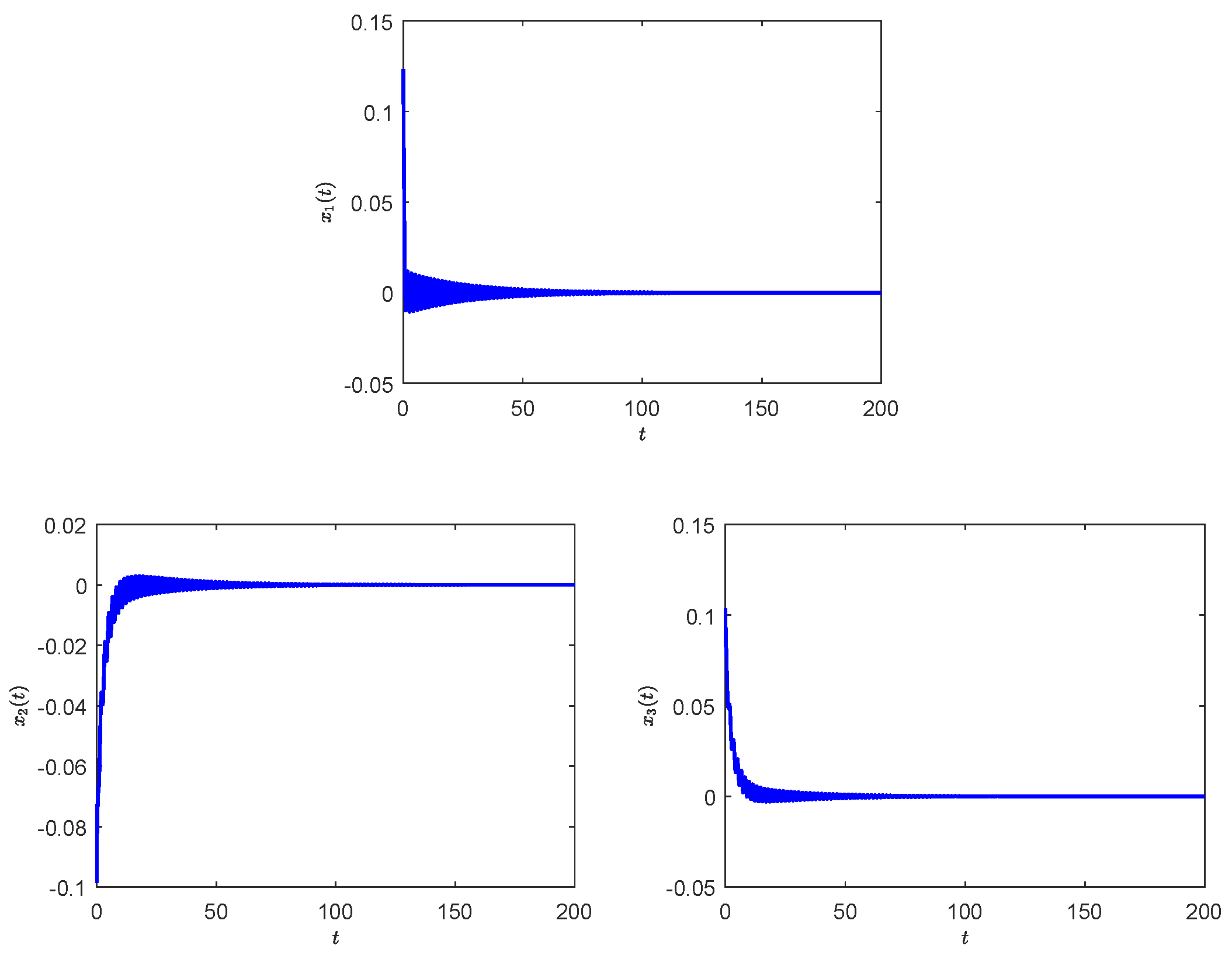
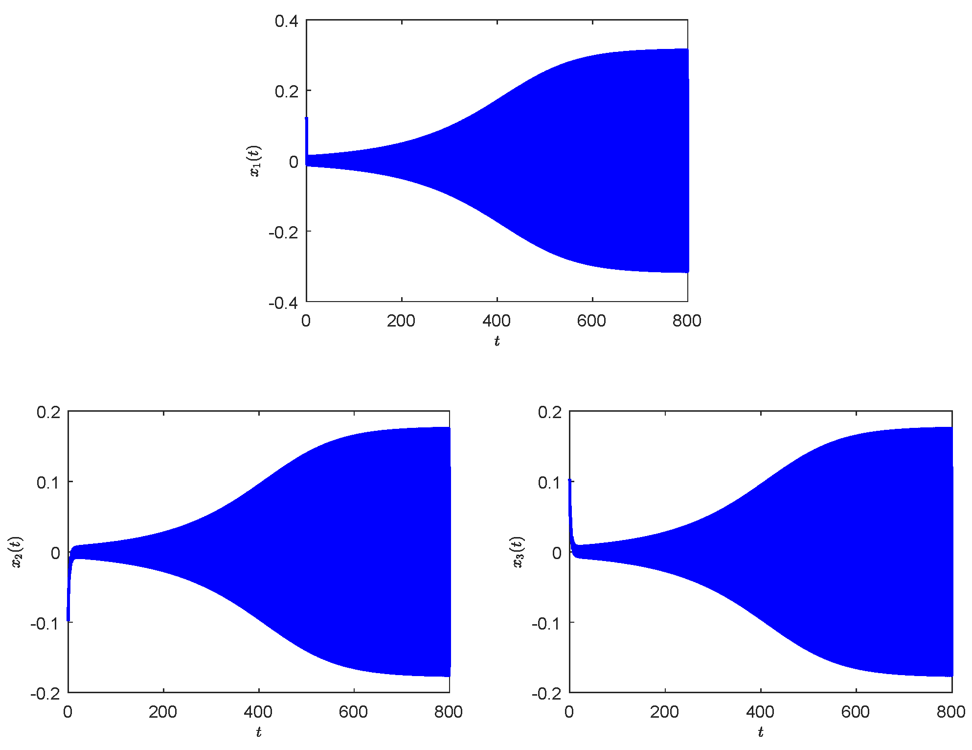
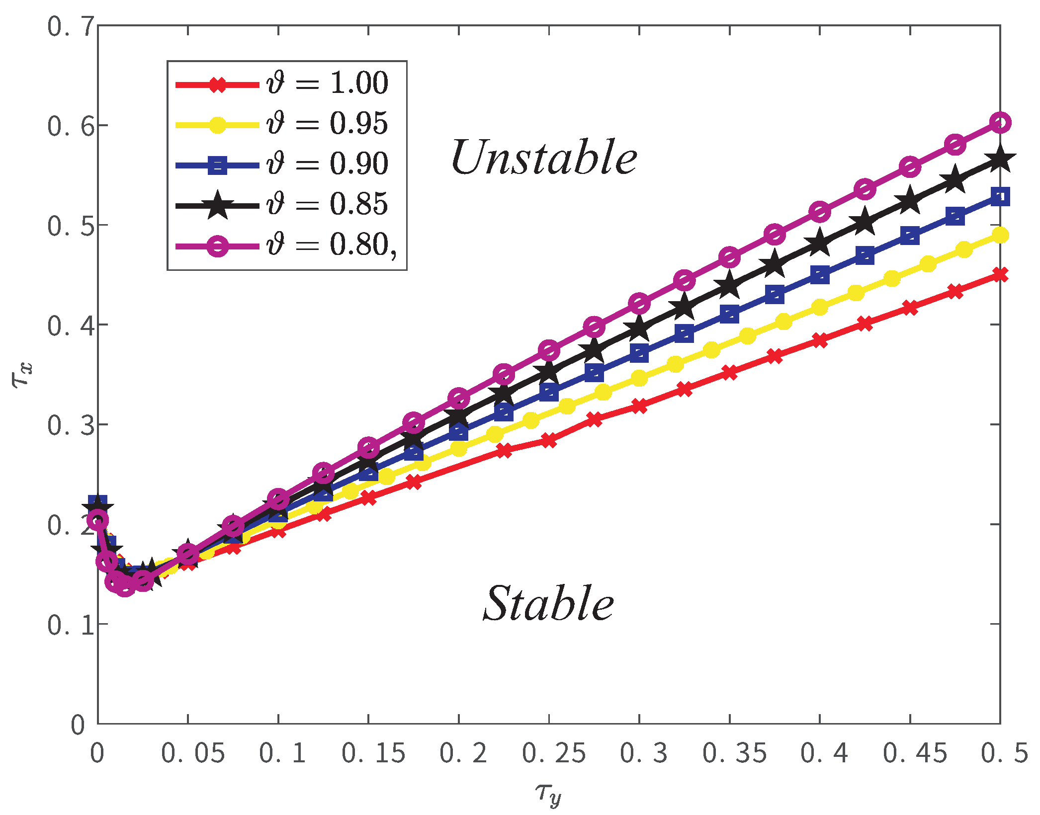
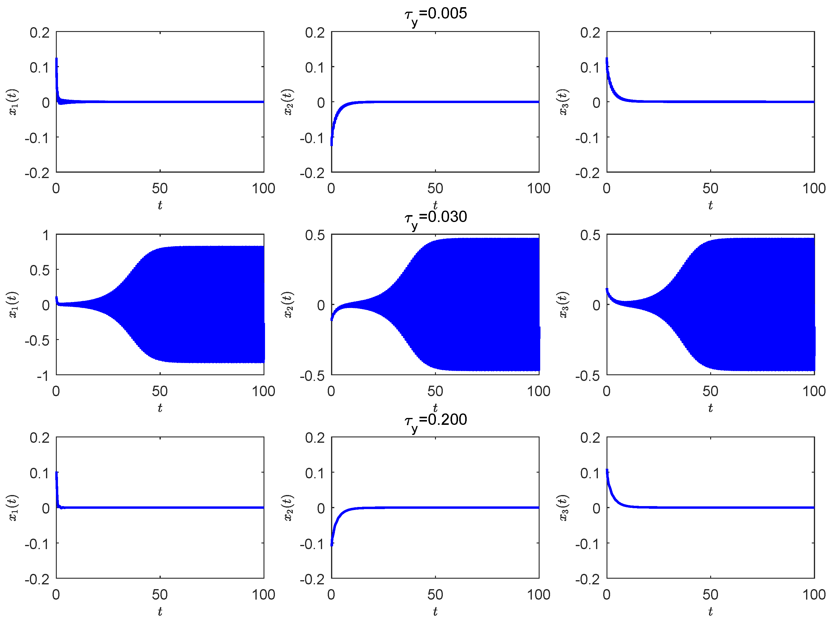
• In contrast to neural networks with only retarded delays, the Hopf bifurcation curve is non-monotonic. This indicates that system (24) with a fixed communication delay can exhibit stability switches and eventually stabilize as the neutral delay increases. We also plotted the time series for ${\tau }_y=0.005$, ${\tau }_y=0.030$, and ${\tau }_y=0.200$, respectively, by fixing ${\tau }_x=0.17$, as shown in Figure 4 which is in excellent agreement with our observation.

Finally, we conducted a sensitivity analysis to show how variations in the parameters affect the Hopf bifurcation point ${\tau }_x^0$. We applied the normalized forward sensitivity index to the positive parameter P, as presented in [46].

$$\begin{array}{c}{\displaystyle Normalizedforwardsensitivityindex=\frac{\partial {\tau }_x^0}{\partial P}·\frac{P}{{\tau }_x^0}.}\hfill \end{array}$$

We adopted the central difference approximation technique to evaluate the following partial derivatives:

$${\displaystyle \frac{\partial {\tau }_x^0}{\partial P}}={\displaystyle \frac{{\tau }_x^0(P+\xi )-{\tau }_x^0(P-\xi )}{2\xi }}+o\left({\xi }^2\right).$$

Accordingly, we defined the sensitivity index $S.I.\left(P\right)$ of the positive parameter P by choosing $ϵ=1\%P$ as below [47]:

$${\displaystyle S.I.\left(P\right)=\frac{{\tau }_x^0\left(1.01P\right)-{\tau }_x^0\left(0.99P\right)}{0.02{\tau }_x^0\left(P\right)}.}$$

(25)

If the parameter P is negative, the result differs from formula (25) by a negative sign. Therefore, we can use formula (25) to evaluate the impacts of the variations in the fractional order and delay-relevant parameters on the stability of system (24). The results are presented in

Table 2. The sensitivity indix $S.I.\left(P\right)$ of ${\tau }_x^0$ about the parameters.

Parameters	$\mathit{S}.\mathit{I}.\left(\mathit{P}\right)$ for ${\mathit{\tau }}_{\mathit{x}}^0$	Parameters	$\mathit{S}.\mathit{I}.\left(\mathit{P}\right)$ for ${\mathit{\tau }}_{\mathit{x}}^0$
$\vartheta$	−1.1851	${\tau }_y$	0.5117
${\beta }_{11}$	0.0541	$d_{11}$	0.0097
${\beta }_{12}$	0.0400	$d_{12}$	−0.0428
${\beta }_{13}$	0.0400	$d_{13}$	−0.0428
${\beta }_{21}$	0.0043	$d_{21}$	−0.0872
${\beta }_{22}$	0.1166	$d_{22}$	−0.1726
${\beta }_{23}$	0.1803	$d_{23}$	−0.4168
${\beta }_{31}$	−0.0043	$d_{31}$	−0.0872
${\beta }_{32}$	0.1803	$d_{32}$	−0.4168
${\beta }_{33}$	0.1166	$d_{33}$	−0.1726

.

A positive (negative) value of the index indicates that an increase (decrease) in the associated parameter enhances the system stability. The magnitude reflects the strength of this relationship. It is observed that the fractional order $\vartheta$ and the neutral delay ${\tau }_y$ are the two most sensitive parameters affecting the bifurcation point ${\tau }_x^0$. In other words, compared to other parameters, small variations in the two parameters can significantly impact the stability of system (24).

4. Conclusions

In this study, we propose a novel delayed fractional neutral tri-neuron network that integrates key factors such as the memory properties of neural networks, communication delay, and neutral delay. By applying the Laplace transformation [43,44], we derived the corresponding characteristic equation. To determine the bifurcation value of the communication delay, we overcame significant mathematical challenges associated with handling the terms ${\mathrm{e}}^{-3s{\tau }_x}$ and ${\mathrm{e}}^{-3s{\tau }_y}$ in the characteristic equation. Our findings reveal that as the communication delay surpasses the bifurcation threshold, the system transitions into an unstable state. Furthermore, sensitivity analysis indicates that neutral delay and fractional order are the two most sensitive parameters affecting the bifurcation value. The simulations showed that increasing the neutral delay induces stability switches.

Despite these insights, several essential and challenging issues remain open for future research. The study of neural networks can be broadly categorized into theoretical research and applied research. Some applications rely heavily on the dynamic properties of the designed neural networks. For instance, the robustness of associative memory is closely tied to the attractive domain of equilibrium points. Our findings offer valuable insights into the stability of equilibrium under fixed parameters, laying a solid foundation for further advancements. A promising direction for future research involves the circuit implementation of memristors to design robust associative memories [48] and hardware implementation to conduct image encryption based on our theoretical framework [49]. Additionally, our approach to calculating the Hopf bifurcation draws inspiration from previous work [43,44], where the authors employed the Caputo derivative and applied the Laplace transform to analyze the associated linear system. It is worth noting that fractional derivatives extend beyond the Caputo definition. The formulation of time delays and characteristic equations can vary significantly under different fractional derivatives, such as the Caputo–Hadamard derivative [50]. Successfully extending our approach to analyze Hopf bifurcations across various fractional derivatives remains a complex mathematical challenge. Addressing these questions is an important avenue for future investigation.

References

1. Bishop, C.M. Neural Networks for Pattern Recognition; Oxford University Press: Oxford, UK, 1995. [Google Scholar]
2. Aggarwal, C.C. Neural Networks and Deep Learning; Springer: Berlin/Heidelberg, Germany, 2018; Volume 10. [Google Scholar]
3. Hopfield, J.J. Neurons with graded response have collective computational properties like those of two-state neurons. Proc. Natl. Acad. Sci. USA 1984, 81, 3088–3092. [Google Scholar] [CrossRef]
4. Marcus, C.M.; Westervelt, R.M. Stability of analog neural networks with delay. Phys. Rev. A 1989, 39, 347. [Google Scholar] [CrossRef]
5. Krstic, M. Delay Compensation for Nonlinear, Adaptive, and PDE Systems; Springer: Berlin/Heidelberg, Germany, 2009. [Google Scholar] [CrossRef]
6. Pahnehkolaei, S.M.A.; Alfi, A.; Machado, J.T. Delay-dependent stability analysis of the QUAD vector field fractional order quaternion-valued memristive uncertain neutral type leaky integrator echo state neural networks. Neural Netw. 2019, 117, 307–327. [Google Scholar] [CrossRef] [PubMed]
7. Lu, Y.X.; Xiao, M.; Liang, J.L.; Chen, J.; Lin, J.X.; Wang, Z.X.; Cao, J.D. Spatiotemporal Evolution of Large-Scale Bidirectional Associative Memory Neural Networks With Diffusion and Delays. IEEE Trans. Syst. Man. Cybern. Syst. 2023, 54, 1388–1400. [Google Scholar] [CrossRef]
8. Wei, J.J.; Ruan, S.G. Stability and bifurcation in a neural network model with two delays. Phys. D 1999, 130, 255–272. [Google Scholar] [CrossRef]
9. Gupta, P.D.; Majee, N.; Roy, A. Stability, bifurcation and global existence of a Hopf-bifurcating periodic solution for a class of three-neuron delayed network models. Nonlinear Anal. Theory Methods Appl. 2007, 67, 2934–2954. [Google Scholar] [CrossRef]
10. Lien, C.H.; Yu, K.W.; Lin, Y.F.; Chung, Y.J.; Chung, L.Y. Global exponential stability for uncertain delayed neural networks of neutral type with mixed time delays. IEEE Trans. Syst. Man. Cybern. B. 2008, 38, 709–720. [Google Scholar] [CrossRef]
11. Song, Q.K.; Zhao, Z.J.; Liu, Y.R.; Alsaadi, F.E. Mean-square input-to-state stability for stochastic complex-valued neural networks with neutral delay. Neurocomputing 2022, 470, 269–277. [Google Scholar] [CrossRef]
12. Zhang, Z.Q.; Liu, W.B.; Zhou, D.M. Global asymptotic stability to a generalized Cohen–Grossberg BAM neural networks of neutral type delays. Neural Netw. 2012, 25, 94–105. [Google Scholar] [CrossRef]
13. Fridman, E. New Lyapunov–Krasovskii functionals for stability of linear retarded and neutral type systems. Syst. Control. Lett. 2001, 43, 309–319. [Google Scholar] [CrossRef]
14. Han, Q.L. Robust stability of uncertain delay-differential systems of neutral type. Automatica 2002, 38, 719–723. [Google Scholar] [CrossRef]
15. Cheng, C.J.; Liao, T.L.; Yan, J.J.; Hwang, C.C. Globally asymptotic stability of a class of neutral-type neural networks with delays. IEEE Trans. Syst. Man. Cybern. B. 2006, 36, 1191–1195. [Google Scholar] [CrossRef]
16. Zhang, H.G.; Liu, Z.W.; Huang, G.B. Novel delay-dependent robust stability analysis for switched neutral-type neural networks with time-varying delays via SC technique. IEEE Trans. Syst. Man. Cybern. B. 2010, 40, 1480–1491. [Google Scholar] [CrossRef]
17. Faydasicok, O. New criteria for global stability of neutral-type Cohen–Grossberg neural networks with multiple delays. Neural Netw. 2020, 125, 330–337. [Google Scholar] [CrossRef] [PubMed]
18. Arik, S. New criteria for stability of neutral-type neural networks with multiple time delays. IEEE Trans. Neural Networks Learn. Syst. 2019, 31, 1504–1513. [Google Scholar] [CrossRef]
19. He, Y.; Liu, G.P.; Rees, D.; Wu, M. Stability analysis for neural networks with time-varying interval delay. IEEE Trans. Neural Netw. 2007, 18, 1850–1854. [Google Scholar] [CrossRef] [PubMed]
20. Dong, T.; Xia, L.M. Stability and Hopf bifurcation of a reaction–diffusion neutral neuron system with time delay. Int. J. Bifurcat. Chaos 2017, 27, 1750214. [Google Scholar] [CrossRef]
21. Park, J.H.; Kwon, O.M.; Lee, S.M. LMI optimization approach on stability for delayed neural networks of neutral-type. Appl. Math. Comput. 2008, 196, 236–244. [Google Scholar] [CrossRef]
22. Feng, J.E.; Xu, S.Y.; Zou, Y. Delay-dependent stability of neutral type neural networks with distributed delays. Neurocomputing 2009, 72, 2576–2580. [Google Scholar] [CrossRef]
23. Zhang, Y.; Li, L.; Huang, J.; Gorbachev, S.; Aravind, R.V. Exploration on bifurcation for an incommensurate five-neuron fractional-order BAM neural network involving multiple delays. Phys. D 2024, 460, 134047. [Google Scholar] [CrossRef]
24. Xu, C.; Zhao, Y.; Lin, J.; Pang, Y.; Liu, Z.; Shen, J.; Liao, M.; Li, P.; Qin, Y. Bifurcation investigation and control scheme of fractional neural networks owning multiple delays. Comp. Appl. Math. 2024, 43, 1–33. [Google Scholar] [CrossRef]
25. Li, S.; Cao, J.; Liu, H.; Huang, C. Delay-dependent parameters bifurcation in a fractional neural network via geometric methods. Appl. Math. Comput. 2024, 478, 128812. [Google Scholar] [CrossRef]
26. Wu, Z.; Cai, Y.; Wang, Z.; Wang, W. Global stability of a fractional order SIS epidemic model. J. Differ. Equations 2023, 352, 221–248. [Google Scholar] [CrossRef]
27. Khalighi, M.; Lahti, L.; Ndaïrou, F.; Rashkov, P.; Torres, D.F. Fractional modelling of COVID-19 transmission incorporating asymptomatic and super-spreader individuals. Math. Biosci. 2025, 380, 109373. [Google Scholar] [CrossRef]
28. Lundstrom, B.N.; Higgs, M.H.; Spain, W.J.; Fairhall, A.L. Fractional differentiation by neocortical pyramidal neurons. Nat. Neurosci. 2008, 11, 1335–1342. [Google Scholar] [CrossRef]
29. Anastasio, T.J. The fractional-order dynamics of brainstem vestibulo-oculomotor neurons. Biol. Cybern. 1994, 72, 69–79. [Google Scholar] [CrossRef]
30. Pu, Y.F.; Yuan, X.; Yu, B. Analog circuit implementation of fractional-order memristor: Arbitrary-order lattice scaling fracmemristor. IEEE Trans. Circuits Syst. I: Regul. Pap. 2018, 65, 2903–2916. [Google Scholar] [CrossRef]
31. Chen, J.J.; Zeng, Z.G.; Jiang, P. Global Mittag-Leffler stability and synchronization of memristor-based fractional-order neural networks. Neural Netw. 2014, 51, 1–8. [Google Scholar] [CrossRef] [PubMed]
32. Cheng, Z. Control of the Bifurcation Behaviors of Delayed Fractional-Order Neural Networks with Cooperation–Competition Topology. Fractal Fract. 2024, 8, 689. [Google Scholar] [CrossRef]
33. Ortigueira, M.D. A factory of fractional derivatives. Symmetry 2024, 16, 814. [Google Scholar] [CrossRef]
34. Valério, D.; Ortigueira, M.D.; Lopes, A.M. How many fractional derivatives are there? Mathematics 2022, 10, 737. [Google Scholar] [CrossRef]
35. Podlubny, I. Fractional Differential Equations: An Introduction to Fractional Derivatives, Fractional Differential Equations, to Methods of Their Solution and Some of Their Applications; Academic Press: New York, NY, USA, 1999. [Google Scholar]
36. Huang, W.; Song, Q.; Zhao, Z.; Liu, Y.; Alsaadi, F.E. Robust stability for a class of fractional-order complex-valued projective neural networks with neutral-type delays and uncertain parameters. Neurocomputing 2021, 450, 399–410. [Google Scholar] [CrossRef]
37. Popa, C.A. Neutral-type and mixed delays in fractional-order neural networks: Asymptotic stability analysis. Fractal Fract. 2022, 7, 36. [Google Scholar] [CrossRef]
38. Huang, C.D.; Liu, H.; Huang, T.W.; Cao, J.D. Bifurcations Due to Different Neutral Delays in a Fractional-Order Neutral-Type Neural Network. IEEE Trans. Emerg. Top. Comput. 2024, 8, 563–575. [Google Scholar] [CrossRef]
39. Kumar, P.; Lee, T.H.; Erturk, V.S. A novel fractional-order neutral-type two-delayed neural network: Stability, bifurcation, and numerical solution. Math. Comput. Simul. 2025, 232, 245–260. [Google Scholar] [CrossRef]
40. Li, L.; Yuan, Y. Dynamics in three cells with multiple time delays. Nonlinear Anal. Real World Appl. 2008, 9, 725–746. [Google Scholar] [CrossRef]
41. Wang, H.; Huang, C.; Liu, S.; Cao, J.; Liu, H. Bifurcation detection of a neutral-type fractional-order delayed neural network via stability switching curve. Nonlinear Dyn. 2025, 113, 3781–3790. [Google Scholar] [CrossRef]
42. Gao, J.; Huang, C.D.; Liu, H. Hopf bifurcations in a fractional-order neural network introducing delays into neutral terms. Eur. Phys. J. Plus. 2024, 139, 1–11. [Google Scholar] [CrossRef]
43. Deng, W.H.; Li, C.P.; Lü, J.H. Stability analysis of linear fractional differential system with multiple time delays. Nonlinear Dyn. 2007, 48, 409–416. [Google Scholar] [CrossRef]
44. Pakzad, M.A.; Pakzad, S.; Nekoui, M.A. On the stability of fractional-order systems of neutral type. J. Comput. Nonlinear Dyn. 2015, 10, 051013. [Google Scholar] [CrossRef]
45. Tuan, H.T.; Thai, H.D.; Garrappa, R. An analysis of solutions to fractional neutral differential equations with delay. Commun. Nonlinear Sci. Numer. Simul. 2021, 100, 105854. [Google Scholar] [CrossRef]
46. Chitnis, N.; Hyman, J.M.; Cushing, J.M. Determining important parameters in the spread of malaria through the sensitivity analysis of a mathematical model. Bull. Math. Biol. 2008, 70, 1272–1296. [Google Scholar] [CrossRef] [PubMed]
47. Li, S.; Huang, C.D.; Yuan, S.L. Hopf bifurcation of a fractional-order double-ring structured neural network model with multiple communication delays. Nonlinear Dyn. 2022, 108, 379–396. [Google Scholar] [CrossRef]
48. Chen, C.; Min, F.; Cai, J.; Bao, H. Memristor synapse-driven simplified Hopfield neural network: Hidden dynamics, attractor control, and circuit implementation. IEEE Trans. Circuits Syst. I Regul. Pap. 2024, 71, 2308–2319. [Google Scholar] [CrossRef]
49. Kong, X.; Yu, F.; Yao, W.; Cai, S.; Zhang, J.; Lin, H. Memristor-induced hyperchaos, multiscroll and extreme multistability in fractional-order HNN: Image encryption and FPGA implementation. Neural Netw. 2024, 171, 85–103. [Google Scholar] [CrossRef]
50. Bounoua, M.D.; Yin, C. Hopf bifurcation in Caputo–Hadamard fractional-order differential system. Fractals 2022, 30, 2250015. [Google Scholar] [CrossRef]
Figure 1. Time series of system (24) with τ x = 0.27 < τ x 0 .
Fractalfract 09 00189 g001
Figure 2. Time series of system (24) with τ x = 0.28 > τ x 0 .
Fractalfract 09 00189 g002
Figure 3. Hopf bifurcation curves and stable and unstable regions in the ( τ x , τ y ) plane for different fractional orders.
Fractalfract 09 00189 g003
Figure 4. Stability switches occur as τ y increases in system (24) with τ x = 0.17 .
Fractalfract 09 00189 g004