Analyzing the Transient Process and the Realizability of Fractional Systems via Intermittent Control

Abstract

In this paper, we have studied the transient process and the realizability of fractional systems via intermittent control. For any system under intermittent control input, a transient oscillation process is inevitable when the input switches, which is irrelevant to mathematical model. But this process is usually neglected when considering the achievements of fractional intermittent control systems as the initial value is changed by the switching input. The obtained theoretical results cannot agree with the real physical model. The input signal is treated as a piecewise signal by means of convolution operation and unit step function, and the output is drawn by convoluting the control input with a time decay function. We have drawn the conclusions that the initial value of the fractional model can not be updated by any outer input and that a transient process must exist that is related to all historic process and the memory property of a fractional system. If the response function of a system is taken as the time decay function, the results obtained are in good agreement with the actual model and can be used to analyze the transient phenomena in nature. Some examples are presented to verify our theoretical achievements.

1. Introduction

For a control system, the aim is to optimize the output performance by designing the control input. The output can be drawn by convoluting the input with the unit impulsive response. The unit impulsive response is an essential property of a system that is irrelevant to its input, and reflects the memory property of all inputs, beginning with the initial time [1,2]. When the input is switched, the input information before this switch still has an effect on the output, and a transient oscillation process is inevitable [3,4,5]. Transient processes are widely presented in many fields such as power, machine, control, etc.

The fractional calculus defined by convolution operation contains all the dynamic information. The initial time of the fractional model denotes the starting point of the historical information [6,7,8]. It can do well with this memory characteristics [9,10] and is a very good tool to study the response property of a system [11,12,13]. Using the fractional model and intermittent control, many achievements have been attained [12,14,15,16,17]. In these achievements, the initial value is usually updated with the intermittent control input [18,19]. This means that the inner memory characteristics are changed by the intermittent control [11,20,21]. But, the memory characteristics are an internal attribute and cannot be changed by any external input. Clearly, the effect of the historical input information on the transient process is neglected, which is inconsistent with the real physical process [22,23,24].

Aiming to address the aforementioned problems, we have studied whether the lower bound can be updated and present a transient process for a fractional system via intermittent control in this paper.

The primary contribution of this article can be summarized as follows:

(1)

By introducing a convolution operation and unit step function, the intermittent signal is treated as a piecewise signal, and the output is drawn by convoluting the control input with a time decay function that is relevant to all historical input information.

(2)

We have drawn the conclusions that the initial value of fractional model cannot be updated by any outer input and that a transient process exists. No signal can make this transient process suddenly disappear.

(3)

We have established a tie between the fractional model and a real physical system via intermittent control. This agrees with the real physical model under intermittent control and can be used to study the transient process in nature.

The rest of this paper is organized as follows. In Section 2, the main problem is formulated. The lower bound of fractional calculus is studied in Section 3. In Section 4, we present the transient process analysis of a fractional system under intermittent control. Some examples are proposed to verify our theoretical analysis in Section 5. Lastly, a conclusion is drawn in Section 6.

Notations:  $\Gamma (\Psi )={\int }_0^{\propto }{e}^{-ϵ}{ϵ}^{\Psi -1}dϵ$ is the Gamma function. Operation ‘*’ denotes the convolution operation.

2. Problem Formulation

For simplicity, we take the synchronization of fractional intermittent control system as an example to begin our analysis.

Generally, in the mentioned papers [21,23,24], a fractional target system tends to be depicted as

$$\begin{array}{cc}\hfill & {}_0{}^{C}D_t^{\Psi }x\left(t\right)=\vartheta \left(x\left(t\right)\right)\hfill \end{array}$$

(1)

and the response system via intermittent control is described as

$$\left\{\begin{array}{c}\begin{array}{cc}\hfill & {}_0{}^{C}D_t^{\Psi }y\left(t\right)=\vartheta \left(y\left(t\right)\right)t\in [t_k,{\varsigma }_k)\hfill \\ \hfill & {}_0{}^{C}D_t^{\Psi }y\left(t\right)=\vartheta \left(y\left(t\right)\right)+u_k\left(t\right)t\in [{\varsigma }_k,t_{k+1})\hfill \end{array}\hfill \end{array}\right.$$

(2)

where $u_k\left(t\right)$ and $t_k$ denote the intermittent control and the k switching time, and ${}_0{}^{C}D_t^{\Psi }x\left(t\right)$ and ${}_0{}^{C}D_t^{\Psi }y\left(t\right)$ represent the Caputo fractional derivative of $x\left(t\right)$ and $y\left(t\right)$ with order $\Psi$, respectively.

From Equations (1) and (2), it is of no doubt that the following error equation should be drawn as

$$\left\{\begin{array}{c}\begin{array}{cc}\hfill & {}_{t_0}{}^{C}D_t^{\Psi }e\left(t\right)=\tilde{\vartheta }\left(e\left(t\right)\right)t\in [t_k,{\varsigma }_k)\hfill \\ \hfill & {}_{t_0}{}^{C}D_t^{\Psi }e\left(t\right)=\tilde{\vartheta }\left(e\left(t\right)\right)+u_k\left(t\right)t\in [{\varsigma }_k,t_{k+1})\hfill \end{array}\hfill \end{array}\right.$$

(3)

where $\tilde{\vartheta }\left(e\left(t\right)\right)=\vartheta \left(y\left(t\right)\right)-\vartheta \left(x\left(t\right)\right)$, $\tau =t_k-t_{k-1}$ is the control period and $\vartheta ={\varsigma }_k-t_k$ is the control width.

But in many results, the following error system is derived as

$$\left\{\begin{array}{c}\begin{array}{cc}\hfill & {}_{t_k}{}^{C}D_t^{\Psi }e\left(t\right)=\tilde{\vartheta }\left(e\left(t\right)\right)t\in [t_k,{\varsigma }_k)\hfill \\ \hfill & {}_{{\varsigma }_k}{}^{C}D_t^{\Psi }e\left(t\right)=\tilde{\vartheta }\left(e\left(t\right)\right)+u_k\left(t\right)t\in [{\varsigma }_k,t_{k+1})\hfill \end{array}\hfill \end{array}\right.$$

(4)

Clearly, ${}_{t_0}{}^{C}D_t^{\Psi }e\left(t\right)$ is usually not equal to ${}_{t_k}{}^{C}D_t^{\Psi }e\left(t\right)$ or ${}_{{\varsigma }_k}{}^{C}D_t^{\Psi }e\left(t\right)$. Why has the lower bound of fractional derivative be updated? How can Equation (4) be obtained from Equations (1) and (2)? From another perspective, when $t_k={\varsigma }_k$ or $u_k\left(t\right)=0$, a fractional intermittent control system becomes a fractional continuous control system and a fractional continuous control system can be taken as a special case of a fractional intermittent control system. Obviously, in this case, Equation (4) is also incorrect.

We cannot help but have this doubt regarding how to update the lower bound, what condition the controller should satisfy to ensure that Equation (4) holds, or what phenomena will occur under intermittent control. But these problems have not been solved up to now.

3. Studying the Lower Bound

3.1. Fractional System Analysis

In the mentioned achievements, the Caputo fractional derivative is adopted. For a function $x\left(t\right)$, its Caputo fractional derivative of order $0<\Psi <1$ is defined as

$$\begin{array}{cc}\hfill {}_{t_0}{}^{C}D_t^{\Psi }x\left(t\right)& ={\displaystyle \frac{1}{\Gamma (1-\Psi )}}{\int }_{t_0}^t{\displaystyle \frac{x^{\prime }\left(\tau \right)}{{(t-\tau )}^{\Psi }}}d\tau \hfill \end{array}$$

(5)

According to the fractional integral, it shows

$$\begin{array}{cc}\hfill x\left(t\right)& =x\left(t_0\right)+{\displaystyle \frac{1}{\Gamma (\Psi )}}{\int }_{t_0}^t{(t-\tau )}^{\Psi -1}{[}_{t_0}^C{D}_{\tau }^{\Psi }x\left(\tau \right)]d\tau \hfill \end{array}$$

(6)

Define ${\mu }_s\left(t\right)$ as unit step function:

$$\begin{array}{c}\hfill {\mu }_s\left(t\right)=\left\{\begin{array}{c}0,t<0,\hfill \\ {\displaystyle \frac{1}{2}},t=0,\hfill \\ 1,t>0\hfill \end{array}\right.\end{array}$$

(7)

According to the convolution operation, we have the following:

$$\begin{array}{cc}\hfill {}_{t_0}{}^{C}D_t^{\Psi }x\left(t\right)& ={\displaystyle \frac{1}{\Gamma (1-\Psi )}}\left[x^{\prime }\left(t\right){\mu }_s(t-t_0)\right]\ast \left[t^{-\Psi }{\mu }_s\left(t\right)\right]\hfill \end{array}$$

(8)

and

$$\begin{array}{cc}\hfill x\left(t\right)& =x\left(t_0\right)+{\displaystyle \frac{1}{\Gamma (\Psi )}}{[}_{t_0}^C{D}_t^{\Psi }x\left(t\right){\mu }_s(t-t_0)]\ast \left[t^{\Psi -1}{\mu }_s\left(t\right)\right]\hfill \end{array}$$

(9)

Any $t_{\ell }>t_0$, from Equation (8), yields

$$\begin{array}{cc}\hfill & {}_{t_0}{}^{C}D_t^{\Psi }x\left(t\right)={\displaystyle \frac{1}{\Gamma (1-\Psi )}}\left[x^{\prime }\left(t\right){\mu }_s(t-t_0)\right]\ast \left[t^{-\Psi }{\mu }_s\left(t\right)\right]\hfill \\ \hfill & ={\displaystyle \frac{1}{\Gamma (1-\Psi )}}\left[x^{\prime }\left(t\right)[{\mu }_s(t-t_0)-{\mu }_s(t-t_{\ell })+{\mu }_s(t-t_{\ell })]\right]\ast \left[t^{-\Psi }{\mu }_s\left(t\right)\right]\hfill \\ \hfill & ={\displaystyle \frac{1}{\Gamma (1-\Psi )}}\{\left[x^{\prime }\left(t\right)[{\mu }_s(t-t_0)-{\mu }_s(t-t_{\ell })]\right]\ast \left[t^{-\Psi }{\mu }_s\left(t\right)\right]\hfill \\ \hfill & +\left[x^{\prime }\left(t\right){\mu }_s(t-t_{\ell })\right]\ast \left[t^{-\Psi }{\mu }_s\left(t\right)\right]\}\hfill \\ \hfill & ={\displaystyle \frac{1}{\Gamma (1-\Psi )}}\left[x^{\prime }\left(t\right)[{\mu }_s(t-t_0)-{\mu }_s(t-t_{\ell })]\right]\ast \left[t^{-\Psi }{\mu }_s\left(t\right)\right]{+}_{t_{\ell }}^C{D}_t^{\Psi }x\left(t\right)\hfill \end{array}$$

(10)

By means of the unit step function, the intermittent control system can be treated as a piecewise system. The lower bound is the start of the memory of fractional calculus and different results can be drawn with different lower bounds. Obviously, ${}_{t_0}{}^{C}D_t^{\Psi }x\left(t\right){\ne }_{t_{\ell }}^C{D}_t^{\Psi }x\left(t\right)$ unless $\left[x^{\prime }\left(t\right)[{\mu }_s(t-t_0)-{\mu }_s(t-t_{\ell })]\right]\ast \left[t^{-\Psi }{\mu }_s\left(t\right)\right]=0$. Equation (4) is also not equal to Equation (3).

From the definition of fractional system, if we suppose that $h\left(t\right)={\displaystyle \frac{1}{\Gamma (\Psi )}}{t}^{\Psi -1}$, the error system from Equations (1) and (2) can be studied with Figure 1. We can also see that there exist a transient process when the control input is an intermittent signal and Equation (4) cannot be directly drawn from Equations (1) and (2).

Since Equation (4) cannot be directly drawn, the question remains as to whether a controller exists or what condition the controller should satisfy to make Equation (4) hold. Let us present our detailed analysis in the next section.

3.2. The Analysis of the Lower Bound

We suppose that ${}_{t_k}{}^{C}D_t^{\Psi }e\left(t\right)=\tilde{\vartheta }\left(e\left(t\right)\right)(t\in [t_k,{\varsigma }_k),k=0,1,2,\cdots )$ in Equation (4) holds and a controller exists $u_k\left(t\right)$ to make Equation (4) correct.

Let us study what condition the controller $u_k\left(t\right)$ should satisfy.

As ${}_{t_k}{}^{C}D_t^{\Psi }e\left(t\right)=\tilde{\vartheta }\left(e\left(t\right)\right)(t\in [t_k,{\varsigma }_k))$ in Equation (4), it is

$$\begin{array}{cc}\hfill e\left(t\right)& =e\left(t_k\right)+{\displaystyle \frac{1}{\Gamma (\Psi )}}{[}_{t_k}^C{D}_t^{\Psi }e\left(t\right){\mu }_s(t-t_k)]\ast \left[t^{\Psi -1}{\mu }_s\left(t\right)\right]\hfill \end{array}$$

(11)

When $t\in [{\varsigma }_k,t_{k+1})$, the switch in Figure 1 is on. Let us analyze what happens.

We can express Equation (4) as

$$\begin{array}{cc}\hfill & {}_{t_k}{}^{C}D_t^{\Psi }e\left(t\right)=\tilde{\vartheta }\left(e\left(t\right)\right)+u_k\left(t\right){\mu }_s(t-{\varsigma }_k)\hfill \end{array}$$

(12)

when $t\in [t_k,t_{k+1})$.

From the fractional integral, we have

$$\begin{array}{cc}\hfill e\left(t\right)& =e\left(t_k\right)+{\displaystyle \frac{1}{\Gamma (\Psi )}}{[}_{t_k}^C{D}_t^{\Psi }e\left(t\right){\mu }_s(t-t_k)]\ast \left[t^{\Psi -1}{\mu }_s\left(t\right)\right]\hfill \\ \hfill & =e\left(t_k\right)+{\displaystyle \frac{1}{\Gamma (\Psi )}}\left[[\tilde{\vartheta }\left(e\left(t\right)\right)+u_k\left(t\right){\mu }_s(t-{\varsigma }_k)]{\mu }_s(t-t_k)\right]\ast \left[t^{\Psi -1}{\mu }_s\left(t\right)\right]\hfill \\ \hfill & =e\left(t_k\right)+{\displaystyle \frac{1}{\Gamma (\Psi )}}\left[\tilde{\vartheta }\left(e\left(t\right)\right){\mu }_s(t-t_k)\right]\ast \left[t^{\Psi -1}{\mu }_{s}y\right][{\mu }_s(t-t_k)-{\mu }_s(t-{\varsigma }_k)\hfill \\ \hfill & +{\mu }_s(t-{\varsigma }_k)]+{\displaystyle \frac{1}{\Gamma (\Psi )}}\left[u_k\left(t\right){\mu }_s(t-{\varsigma }_k)\right]\ast \left[t^{\Psi -1}{\mu }_s\left(t\right)\right]\hfill \\ \hfill & =e\left(t_k\right)+{\displaystyle \frac{1}{\Gamma (\Psi )}}\left[\tilde{\vartheta }\left(e\left(t\right)\right){\mu }_s(t-t_k)\right]\ast \left[t^{\Psi -1}{\mu }_s\left(t\right)\right][{\mu }_s(t-t_k)-{\mu }_s(t-{\varsigma }_k)]\hfill \\ \hfill & +{\displaystyle \frac{1}{\Gamma (\Psi )}}\left[\tilde{\vartheta }\left(e\left(t\right)\right){\mu }_s(t-t_k)\right]\ast \left[t^{\Psi -1}{\mu }_s\left(t\right)\right]{\mu }_s(t-{\varsigma }_k)\hfill \\ \hfill & +{\displaystyle \frac{1}{\Gamma (\Psi )}}\left[u_k\left(t\right){\mu }_s(t-{\varsigma }_k)\right]\ast \left[t^{\Psi -1}{\mu }_s\left(t\right)\right]\hfill \end{array}$$

(13)

The above equation shows that the output is relevant to the information before the switching time ${\varsigma }_k$ and the memory property of a system cannot be changed by any outer input.

When $t={\varsigma }_k$, we obtain

$$\begin{array}{cc}\hfill e\left({\varsigma }_k\right)& =e\left(t_k\right)+{\displaystyle \frac{1}{\Gamma (\Psi )}}\left[\tilde{\vartheta }\left(e\left(t\right)\right){\mu }_s(t-t_k)\right]\ast \left[t^{\Psi -1}{\mu }_s\right]{|}_{t={\varsigma }_k}\hfill \\ \hfill & =e\left(t_k\right)+{\displaystyle \frac{1}{\Gamma (\Psi )}}\left[\tilde{\vartheta }\left(e\left(t\right)\right){\mu }_s(t-t_k)\right]\ast \left[t^{\Psi -1}{\mu }_s\left(t\right)\right][{\mu }_s(t-t_k)-{\mu }_s(t-{\varsigma }_k)]\hfill \end{array}$$

(14)

From Equation (13), when $t>{\varsigma }_k$, it yields

$$\begin{array}{cc}\hfill e\left(t\right)& =e\left({\varsigma }_k\right)+{\displaystyle \frac{1}{\Gamma (\Psi )}}\left[\tilde{\vartheta }\left(e\left(t\right)\right)[{\mu }_s(t-t_k)-{\mu }_s(t-{\varsigma }_k))\right]]\ast \left[t^{\Psi -1}{\mu }_s\left(t\right)\right]{\mu }_s(t-{\varsigma }_k)\hfill \\ \hfill & +{\displaystyle \frac{1}{\Gamma (\Psi )}}\left[(\tilde{\vartheta }\left(e\left(t\right)\right)+u_k\left(t\right)){\mu }_s(t-{\varsigma }_k)\right]\ast \left[t^{\Psi -1}{\mu }_s\left(t\right)\right]\hfill \end{array}$$

(15)

But, from Equation (4), it also obtains

$$\begin{array}{cc}\hfill e\left(t\right)& =e\left({\varsigma }_k\right)+{\displaystyle \frac{1}{\Gamma (\Psi )}}\left[(\tilde{\vartheta }\left(e\left(t\right)\right)+u_k\left(t\right)){\mu }_s(t-{\varsigma }_k)\right]\ast \left[t^{\Psi -1}{\mu }_s\left(t\right)\right]\hfill \end{array}$$

(16)

when $t>{\varsigma }_k$.

Subtract Equation (16) from Equation (15) to yield

$$\begin{array}{cc}\hfill & 0\equiv e\left({\varsigma }_k\right)+{\displaystyle \frac{1}{\Gamma (\Psi )}}[\tilde{\vartheta }\left(e\left(t\right)\right)[{\mu }_s(t-t_k)-{\mu }_s(t-{\varsigma }_k))]]\ast \left[t^{\Psi -1}{\mu }_s\left(t\right)\right]{\mu }_s(t-{\varsigma }_k)\hfill \\ \hfill & +{\displaystyle \frac{1}{\Gamma (\Psi )}}\left[(\tilde{\vartheta }\left(e\left(t\right)\right)+u_k\left(t\right)){\mu }_s(t-{\varsigma }_k)\right]\ast \left[t^{\Psi -1}{\mu }_s\left(t\right)\right]-\{e\left({\varsigma }_k\right)\hfill \\ \hfill & +{\displaystyle \frac{1}{\Gamma (\Psi )}}\left[(\tilde{\vartheta }\left(e\left(t\right)\right)+u_k\left(t\right)){\mu }_s(t-{\varsigma }_k)\right]\ast \left[t^{\Psi -1}{\mu }_s\left(t\right)\right]\}\hfill \\ \hfill & ={\displaystyle \frac{1}{\Gamma (\Psi )}}[\tilde{\vartheta }\left(e\left(t\right)\right)[{\mu }_s(t-t_k)-{\mu }_s(t-{\varsigma }_k))]]\ast \left[t^{\Psi -1}{\mu }_s\left(t\right)\right]{\mu }_s(t-{\varsigma }_k)\hfill \end{array}$$

(17)

when $t>{\varsigma }_k$.

When $t>{\varsigma }_k$, take the integer derivative of the right part of Equation (17) to obtain

$$\begin{array}{cc}\hfill & {\displaystyle \frac{d}{dt}}\{{\displaystyle \frac{1}{\Gamma (\Psi )}}[\tilde{\vartheta }\left(e\left(t\right)\right)[{\mu }_s(t-t_k)-{\mu }_s(t-{\varsigma }_k))]]\ast \left[t^{\Psi -1}{\mu }_s\left(t\right)\right]{\mu }_s(t-{\varsigma }_k)\}\hfill \\ \hfill & =\{{\displaystyle \frac{1}{\Gamma (\Psi )}}[\tilde{\vartheta }\left(e\left(t\right)\right)[{\mu }_s(t-t_k)-{\mu }_s(t-{\varsigma }_k))]]\ast {\displaystyle \frac{d}{dt}}\left[t^{\Psi -1}{\mu }_s\left(t\right)\right]{\mu }_s(t-{\varsigma }_k)\}\hfill \\ \hfill & \not\equiv 0,\hfill \end{array}$$

(18)

which contradicts with Equation (17). This shows that no controller $u_k\left(t\right)$ can make both Equations (16) and (15) hold. Equation (4) cannot hold for ever. The lower bound of the fractional cannot be changed by any outer input.

For any physical system, a transient process is inevitable when the input signal switches between different states. If the lower bound is changed by the intermittent input, the transient process is neglected, which is inconsistent with the real physical process.

Remark 1. 

In [12,14,15,16,17,18,19], the lower bound is updated with the control input and the output is irrelevant to the historical process. In our paper, we have proved that no signal can make the historical signal change and that the initial value of the fractional model cannot updated.

4. The Analysis of the Transient Process

According to Equation (3), the error system under intermittent control can be expressed as

$$\begin{array}{cc}\hfill & {}_{t_0}{}^{C}D_t^{\Psi }e\left(t\right)=\sum _{i=0}^k(\tilde{\vartheta }\left(e\left(t\right)\right)+u_i\left(t\right))({\mu }_s(t-{\varsigma }_i)-{\mu }_s(t-t_{i+1}))\hfill \end{array}$$

(19)

when $t_k<t<t_{k+1}$.

When $t_k<t<{\varsigma }_k$, we obtain $e\left(t\right)$ as

$$\begin{array}{cc}\hfill e\left(t\right)& =e\left(t_0\right)+{\displaystyle \frac{1}{\Gamma (\Psi )}}\left[\sum _{i=0}^k(\tilde{\vartheta }\left(e\left(t\right)\right)+u_i\left(t\right)({\mu }_s(t-{\varsigma }_i)-{\mu }_s(t-t_{i+1})))\right]\ast \left[t^{\Psi -1}{\mu }_s\left(t\right)\right]\hfill \\ \hfill & =e\left(t_0\right)+{\displaystyle \frac{1}{\Gamma (\Psi )}}\{\sum _{i=0}^{k-1}\left[(\tilde{\vartheta }\left(e\left(t\right)\right)+u_i\left(t\right)({\mu }_s(t-{\varsigma }_i)-{\mu }_s(t-t_{i+1})))\right]\hfill \\ \hfill & ({\mu }_s(t-t_0)-{\mu }_s(t-t_k))\}\ast \left[t^{\Psi -1}{\mu }_s\left(t\right)\right][({\mu }_s(t-t_0)-{\mu }_s(t-t_k))+{\mu }_s(t-t_k)]\hfill \\ \hfill & +{\displaystyle \frac{1}{\Gamma (\Psi )}}\left[\tilde{\vartheta }\left(e\left(t\right)\right){\mu }_s(t-t_k)\right]\ast \left[t^{\Psi -1}{\mu }_s\left(t\right)\right]\hfill \\ \hfill & =e\left(t_0\right)+\{{\displaystyle \frac{1}{\Gamma (\Psi )}}\{\sum _{i=0}^{k-1}\left[(\tilde{\vartheta }\left(e\left(t\right)\right)+u_i\left(t\right)({\mu }_s(t-{\varsigma }_i)-{\mu }_s(t-t_{i+1})))\right]\hfill \\ \hfill & ({\mu }_s(t-t_0)-{\mu }_s(t-t_k))\}\ast \left[t^{\Psi -1}{\mu }_s\left(t\right)\right]\}\left[({\mu }_s(t-t_0)-{\mu }_s(t-t_k))\right]\hfill \\ \hfill & +{\displaystyle \frac{1}{\Gamma (\Psi )}}\left[\tilde{\vartheta }\left(e\left(t\right)\right){\mu }_s(t-t_k)\right]\ast \left[t^{\Psi -1}{\mu }_s\left(t\right)\right]\hfill \\ \hfill & +\{{\displaystyle \frac{1}{\Gamma (\Psi )}}\{\sum _{i=0}^{k-1}\left[(\tilde{\vartheta }\left(e\left(t\right)\right)+u_i\left(t\right)({\mu }_s(t-{\varsigma }_i)-{\mu }_s(t-t_{i+1})))\right]\hfill \\ \hfill & ({\mu }_s(t-t_0)-{\mu }_s(t-t_k))\}\ast \left[t^{\Psi -1}{\mu }_s\left(t\right)y\right]\}{\mu }_s(t-t_k))\hfill \\ \hfill & =e\left(t_k\right)+{\displaystyle \frac{1}{\Gamma (\Psi )}}\left[\tilde{\vartheta }\left(e\left(t\right)\right){\mu }_s(t-t_k)\right]\ast \left[t^{\Psi -1}{\mu }_s\left(t\right)\right]\hfill \\ \hfill & +\{{\displaystyle \frac{1}{\Gamma (\Psi )}}\{\sum _{i=0}^{k-1}\left[(\tilde{\vartheta }\left(e\left(t\right)\right)+u_i\left(t\right)({\mu }_s(t-{\varsigma }_i)-{\mu }_s(t-t_{i+1})))\right]\hfill \\ \hfill & ({\mu }_s(t-t_0)-{\mu }_s(t-t_k))\}\ast \left[t^{\Psi -1}{\mu }_s\right]\}{\mu }_s(t-t_k))\hfill \end{array}$$

(20)

where $e\left(t_k\right)=e\left(t_0\right)+\{{\displaystyle \frac{1}{\Gamma (\Psi )}}\left\{{\displaystyle \sum _{i=0}^{k-1}}\left[(\tilde{\vartheta }\left(e\left(t\right)\right)+u_i\left(t\right)({\mu }_s(t-{\varsigma }_i)-{\mu }_s(t-t_{i+1})))\right]({\mu }_s(t-t_0)-{\mu }_s(t-t_k))\right\}\ast \left[t^{\Psi -1}{\mu }_s\left(t\right)\right]\}\left[({\mu }_s(t-t_0)-{\mu }_s(t-t_k))\right]$. This shows that the output relates to both the current input and all historical input as its memory property.

Define $e_{t_k}^{St}\left(t\right)=e\left(t_k\right)+{\displaystyle \frac{1}{\Gamma (\Psi )}}\left[\tilde{\vartheta }\left(e\left(t\right)\right){\mu }_s(t-t_k)\right]\ast \left[t^{\Psi -1}{\mu }_s\left(t\right)\right]$, which is the steady item and relevant to the initial value $e\left(t_k\right)$ and ${}_{t_0}{}^{C}D_t^{\Psi }e\left(t\right)$ after the time $t_k$, and $e_{t_k}^{Tr}\left(t\right)=\{{\displaystyle \frac{1}{\Gamma (\Psi )}}\left\{{\displaystyle \sum _{i=0}^{k-1}}\left[(\tilde{\vartheta }\left(e\left(t\right)\right)+u_i\left(t\right)({\mu }_s(t-{\varsigma }_i)-{\mu }_s(t-t_{i+1})))\right]({\mu }_s(t-t_0)-{\mu }_s(t-t_k))\right\}\ast \left[t^{\Psi -1}{\mu }_s\left(t\right)\right]\}{\mu }_s(t-t_k))$, which is the transient item and relevant to all historic information before the time $t_k$.

Note 1. As $e_{t_k}^{Tr}\left(t\right)$ may be greater or less than 0, $e\left(t\right)$ may be less or greater than $e\left(t_k\right)$.

When $0<t\le t_k$, there must exist M, satisfying $-M\le \left\{{\displaystyle \sum _{i=0}^{k-1}}\left[(\tilde{\vartheta }\left(e\left(t\right)\right)+u_i\left(t\right)({\mu }_s(t-{\varsigma }_i)-{\mu }_s(t-t_{i+1})))\right]({\mu }_s(t-t_0)-{\mu }_s(t-t_k))\right\}\le M$. Then, we obtain

$$\begin{array}{cc}\hfill & -M({\mu }_s(t-t_0)-{\mu }_s(t-t_k))\ast \left[t^{\Psi -1}{\mu }_s\left(t\right)\right]\le e_{t_k}^{Tr}\left(t\right)\hfill \\ \hfill & \le M({\mu }_s(t-t_0)-{\mu }_s(t-t_k))\ast \left[t^{\Psi -1}{\mu }_s\left(t\right)\right]\hfill \end{array}$$

(21)

Note 2. There exists a transient process for a fractional system under intermittent control. The transient item is limited and its limit is presented as Equation (21).

5. Examples

In this section, some examples are proposed to verify our theoretical analysis.

Example 1. 

Suppose that $x\left(t\right)\in R$, satisfying

$$\begin{array}{cc}\hfill & {}_0{}^{C}D_t^{0.3}x\left(t\right)=\left\{\begin{array}{c}cx\left(t\right),0<t\le 1\hfill \\ 0,t>1\hfill \end{array}\right.\hfill \end{array}$$

(22)

When $1<t$, from Equation (4), it yields

$$\begin{array}{cc}\hfill x\left(t\right)& =x\left(1\right)+{\displaystyle \frac{1}{\Gamma \left(0.3\right)}}\left[0\right]\ast \left[t^{0.3-1}{\mu }_s\left(t\right)\right]\hfill \\ \hfill & +\{{\displaystyle \frac{1}{\Gamma \left(0.3\right)}}\left\{kx\left(t\right)({\mu }_s\left(t\right)-{\mu }_s(t-1))\right\}\ast \left[t^{0.3-1}{\mu }_s\left(t\right)\right]\}{\mu }_s(t-1))\hfill \\ \hfill & =x\left(1\right)+\{{\displaystyle \frac{1}{\Gamma \left(0.3\right)}}\left\{kx\left(t\right)({\mu }_s\left(t\right)-{\mu }_s(t-1))\right\}\ast \left[t^{0.3-1}{\mu }_s\left(t\right)\right]\}{\mu }_s(t-1))\hfill \end{array}$$

(23)

Set $x\left(0\right)=1$, and c is taken as 1 and $-1$, respectively. When $t>1$, ${\displaystyle \frac{d}{dt}}x\left(t\right)=c\{{\displaystyle \frac{1}{\Gamma \left(0.3\right)}}\left\{x\left(t\right)({\mu }_s\left(t\right)-{\mu }_s(t-1))\right\}\ast \left[{\displaystyle \frac{d}{dt}}x\left(t\right)\left(t^{0.3-1}{\mu }_s\left(t\right)\right)\right]{\mu }_s(t-1)\}$.

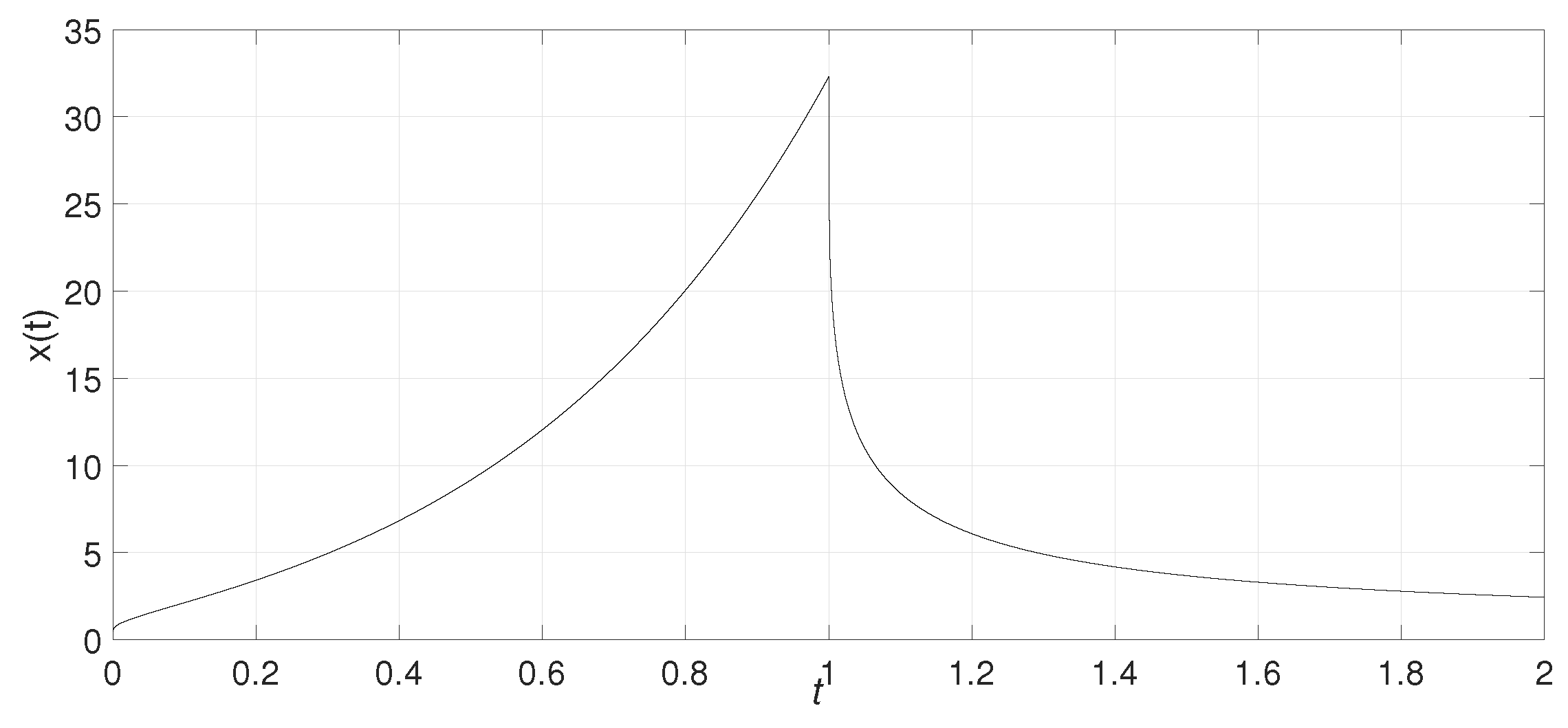
Then, when $c>0$ and $x\left(t\right)>0(0<t<1)$, we have ${\displaystyle \frac{d}{dt}}x\left(t\right)<0$, and $x\left(t\right)$ monotonically decreases when $t>1$, just as in Figure 2.

When $c<0$ and $x\left(t\right)>0(0<t<1)$, we have ${\displaystyle \frac{d}{dt}}x\left(t\right)>0$, and $x\left(t\right)$ monotonically increases when $t>1$, just as in Figure 3.

From the simulations, we can see that the output does not disappear immediately as the input disappears and that there is a transient process. This transient process varies with different historical processes.

Example 2. 

Suppose that $x\left(t\right),y\left(t\right)\in R$, $\vartheta \left(x\left(t\right)\right)=k_{1}x\left(t\right)$, $u_k\left(t\right)=k_2(y\left(t\right)-x\left(t\right))$, $t_k=0.2k$, and ${\varsigma }_k=0.2k+0.1$.

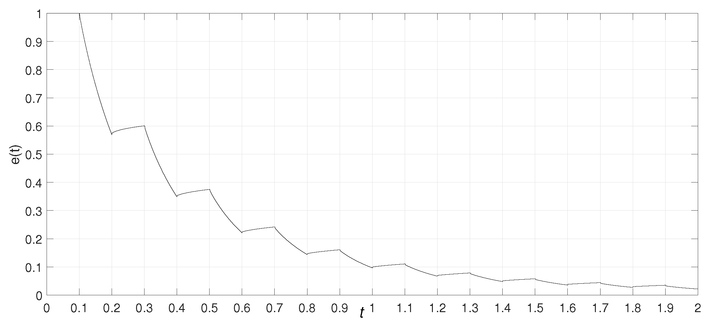
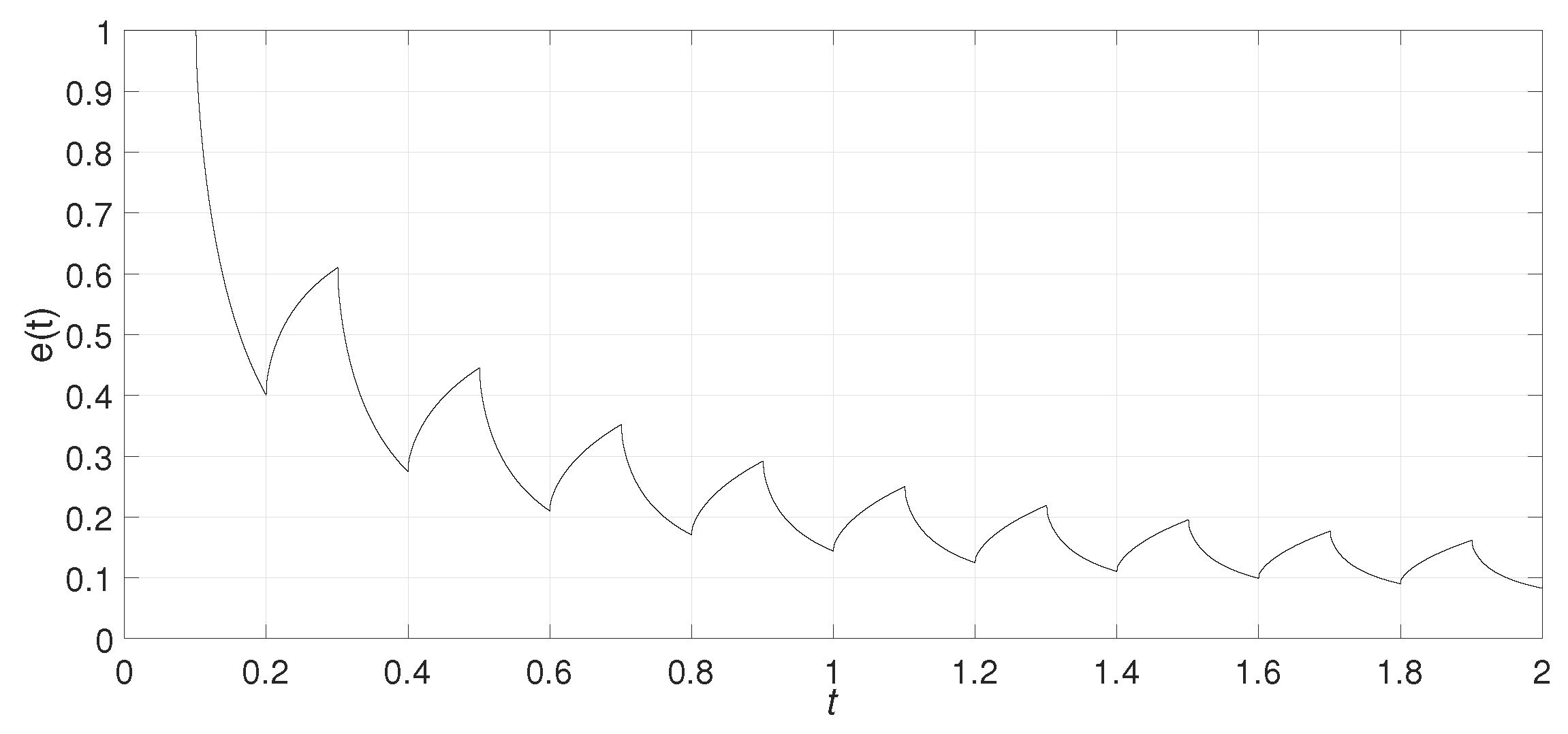
From Equations (1) and (2), it yields

$$\begin{array}{cc}\hfill & {}_0{}^{C}D_t^{\Psi }x\left(t\right)=k_{1}x\left(t\right)\hfill \end{array}$$

(24)

and

$$\left\{\begin{array}{c}\begin{array}{ccc}\hfill & {}_0{}^{C}D_t^{\Psi }y\left(t\right)=k_{1}y\left(t\right)\hfill & \hfill t\in [0.2k,0.2k+0.1)\\ \hfill & {}_0{}^{C}D_t^{\Psi }y\left(t\right)=k_{1}y\left(t\right)+k_2(y\left(t\right)-x\left(t\right))\hfill & \hfill t\in [0.2k+0.1,0.2(k+1\left)\right)\end{array}\hfill \end{array}\right.$$

(25)

Then, the error system is expressed as

$$\left\{\begin{array}{c}\begin{array}{ccc}\hfill & {}_{t_0}{}^{C}D_t^{\Psi }e\left(t\right)=k_{1}e\left(t\right)\hfill & \hfill t\in [0.2k,0.2k+0.1)\\ \hfill & {}_{t_0}{}^{C}D_t^{\Psi }e\left(t\right)=k_{1}e\left(t\right)+k_{2}e\left(t\right)\hfill & \hfill t\in [0.2k+0.1,0.2(k+1\left)\right)\end{array}\hfill \end{array}\right.$$

(26)

Take $k_1=-5$, $k_2=5$. If Equation (4) is correct, we have $e\left(t\right)=e\left(0.2k\right)E_{\Psi }(0\ast {(t-\left(0.2k\right))}^{\Psi })=e\left(0.2k\right)$ when $t\in [0.2k,0.2k+0.1)$ and $e\left(t\right)=e(0.2k+0.1)E_{\Psi }(-5\ast {(t-(0.2k+0.1))}^{\Psi })$ when $t\in [0.2k+0.1,0.2k+0.2)$.

We set $\Psi =0.95$, $\Psi =0.7$, and $\Psi =0.22$, respectively. The numerical simulations are shown in Figure 4 and Figure 5 with $\Psi =0.95$, Figure 6 and Figure 7 with $\Psi =0.7$, and Figure 8 and Figure 9 with $\Psi =0.22$. From Figure 4, Figure 6, and Figure 8, we can clearly see that $e\left(t\right)(t\in [0.2k,0.2k+0.1\left)\right)$ is not constant, which indicates that Equation (4) is incorrect. Figure 5, Figure 7, and Figure 9 show that this system is stable.

These numerical simulations verify that the output of a fractional system under intermittent control consists of the transient item and steady item. The transient item decays with time, and relates to the historical dynamic information and the response characteristics. Different transient processes exist for different systems and different historical processes. This agrees with the real system under intermittent control in nature.

Remark 2. 

Compared with [12,15,16,17,18,19,25,26], our research shows that there exist a transient process when the input switches. This agrees with the transient process in nature.

6. Conclusions

In nature, a transient process is inevitable for any system under intermittent control. This transient process varies with the system memory property, history dynamic process, and the control input, and is irrelevant to mathematical model. This process should be considered no matter what mathematical model is adapted.

This process is usually neglected by the fractional model. Aiming to address this problem, we have established a connection between a fractional model and physical system. Our research shows that no signal can make this transient process suddenly disappear and that the lower bound of fractional model can not be updated. We present a novel approach to studying the transient process. It is helpful to optimize the transient process and enhance the control accuracy. It can be widely applied in the study of the transient oscillation caused by power switching and machining.

References

- Shan, W.; Wang, Y.; Tang, W. Fractional order internal model pid control for pulp batch cooking process. J. Chem. Eng. Jpn. 2023, 56, 2201288. [Google Scholar] [CrossRef]
- Hu, J.-B.; Zhao, L.-D.; Lu, G.-P.; Zhang, S.-B. The stability and control of fractional nonlinear system with distributed time delay. Appl. Math. Model. 2016, 40, 3257–3263. [Google Scholar] [CrossRef]
- Zhu, Q. Event-triggered sampling problem for exponential stability of stochastic nonlinear delay systems driven by levy processes. IEEE Trans. Autom. Control 2025, 70, 1176–1183. [Google Scholar] [CrossRef]
- Talebi, S.; Godsill, S.; Mandic, D. Filtering structures for α-stable systems. IEEE Control Syst. Lett. 2023, 7, 553–558. [Google Scholar] [CrossRef]
- Hu, J.; Li, S.; Jin, Z.; Chao, X. Studying the transient process of an intermittent control system from its response property. Commun. Nonlinear Sci. Numer. Simul. 2024, 139, 108309. [Google Scholar] [CrossRef]
- Hu, L.; Yu, H. Event-triggered finite-time tracking control for fractional-order multi-agent systems with input saturation and constraints. Appl. Artif. Intell. 2023, 37, 2166689. [Google Scholar] [CrossRef]
- Zvyagin, V.; Zvyagin, A.; Ustiuzhaninova, A. Optimal feedback control problem for the fractional voigt-a model. Mathematics 2020, 8, 1197. [Google Scholar] [CrossRef]
- Gladkov, S.O. On the question of self-organization of population dynamics on earth. Biophysics 2021, 66, 858–866. [Google Scholar] [CrossRef]
- Meng, X.; Gao, C.; Jiang, B.; Karimi, H.R. An event-triggered sliding mode control mechanism to exponential consensus of fractional-order descriptor nonlinear multi-agent systems. Proc. Inst. Mech. Eng. Part I J. Syst. Control Eng. 2024, 238, 532–544. [Google Scholar] [CrossRef]
- Zhao, L.; Chen, Y. Comments on “a novel approach to approximate fractional derivative with uncertain conditions”. Chaos Solitons Fractals 2022, 154, 111651. [Google Scholar] [CrossRef]
- Xu, Y.; Lin, T.; Feng, J. Exponential stabilization for fractional intermittent controlled multi-group models with dispersal. Neurocomputing 2021, 445, 220–230. [Google Scholar] [CrossRef]
- Yang, Y.; He, Y.; Wu, M. Intermittent control strategy for synchronization of fractional-order neural networks via piecewise lyapunov function method. J. Frankl. Inst.-Eng. Appl. Math. 2019, 356, 4648–4676. [Google Scholar] [CrossRef]
- Li, X.Y.; Wu, K.-N.; Liu, X.-Z. Mittag-leffler stabilization for short memory fractional reaction-diffusion systems via intermittent boundary control. Appl. Math. Comput. 2023, 449, 127959. [Google Scholar] [CrossRef]
- Wu, C.; Liu, X. Lyapunov and external stability of caputo fractional order switching systems. Nonlinear Anal.-Hybrid Syst. 2019, 34, 131–146. [Google Scholar] [CrossRef]
- Hui, M.; Wei, C.; Zhang, J.; Iu, H.H.-C.; Yao, R.; Bai, L. Finite-time synchronization of fractional-order memristive neural networks via feedback and periodically intermittent control. Commun. Nonlinear Sci. Numer. Simul. 2023, 116, 106822. [Google Scholar] [CrossRef]
- Liu, X.-Z.; Wu, K.-N.; Ahn, C.K. Intermittent boundary control for synchronization of fractional delay neural networks with diffusion terms. IEEE Trans. Syst. Man Cybern. Syst. 2023, 53, 2900–2912. [Google Scholar] [CrossRef]
- Chen, G.; Yang, Y. Stability of a class of nonlinear fractional order impulsive switched systems. Trans. Inst. Meas. Control 2017, 39, 781–790. [Google Scholar] [CrossRef]
- Li, H.-L.; Hu, C.; Jiang, H.; Teng, Z.; Jiang, Y.-L. Synchronization of fractional-order complex dynamical networks via periodically intermittent pinning control. Chaos Solitons Fractals 2017, 103, 357–363. [Google Scholar] [CrossRef]
- Xu, Y.; Li, Y.; Li, W. Graph-theoretic approach to synchronization of fractional-order coupled systems with time-varying delays via periodically intermittent control. Chaos Solitons Fractals 2019, 121, 108–118. [Google Scholar] [CrossRef]
- Zhao, L. A note on “cluster synchronization of fractional-order directed networks via intermittent pinning control”. Phys. A-Stat. Mech. Its Appl. 2021, 561, 125150. [Google Scholar] [CrossRef]
- Cai, S.; Hou, M. Quasi-synchronization of fractional-order heterogeneous dynamical networks via aperiodic intermittent pinning control. Chaos Solitons Fractals 2021, 146, 110901. [Google Scholar] [CrossRef]
- Meng, F.; Zeng, X.; Wang, Z.; Wang, X. Anti-synchronization of fractional-order chaotic circuit with memristor via periodic intermittent control. Adv. Math. Phys. 2020, 2020, 5158489. [Google Scholar] [CrossRef]
- Xu, Y.; Gao, S.; Li, W. Exponential stability of fractional-order complex multi-links networks with aperiodically intermittent control. IEEE Trans. Neural Netw. Learn. Syst. 2021, 32, 4063–4074. [Google Scholar] [CrossRef] [PubMed]
- Wang, Y.; Wu, Z. Cluster synchronization in variable-order fractional community network via intermittent control. Mathematics 2021, 9, 2596. [Google Scholar] [CrossRef]
- Ding, K.; Zhu, Q. Fuzzy intermittent extended dissipative control for delayed distributed parameter systems with stochastic disturbance: A spatial point sampling approach. IEEE Trans. Fuzzy Syst. 2022, 30, 1734–1749. [Google Scholar] [CrossRef]
- Ding, K.; Zhu, Q. Intermittent static output feedback control for stochastic delayed-switched positive systems with only partially measurable information. IEEE Trans. Autom. Control 2023, 68, 8150–8157. [Google Scholar] [CrossRef]