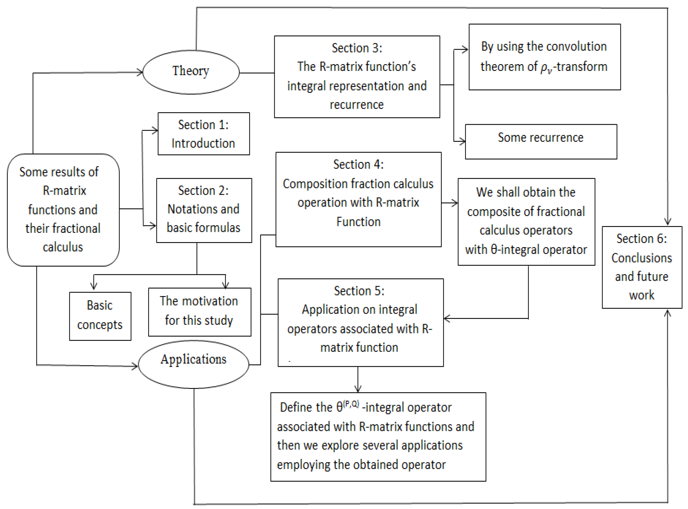
Some Results of R-Matrix Functions and Their Fractional Calculus

Abstract

In this study, we explore various fractional integral properties of R-matrix functions using the Hilfer fractional derivative operator within the framework of fractional calculus. We introduce the $\theta$ integral operator and extend its definition to include the R matrix functions. The composition of Riemann–Liouville fractional integral and differential operators is determined using the $\theta$-integral operator. Additionally, we investigate the compositional properties of $\theta$-integral operators, and we establish their inversion, offering new insights into their structural and functional characteristics.

1. Introduction

Fractional analysis, a branch of mathematics concerned with generalizations of classical calculus to non-integer orders, has garnered significant attention in recent decades. Its foundation lies in extending the concepts of differentiation and integration to fractional, real, or even complex orders, thereby enabling the modeling of phenomena characterized by memory, hereditary properties, and anomalous diffusion. This mathematical framework finds applications in diverse fields, including physics, engineering, biology, and finance [1]. Fractional analysis has a profound connection with special functions, as many solutions to fractional differential equations are expressed in terms of such functions. For instance, Mittag–Leffler functions: Often regarded as the “fractional exponential function”, Mittag–Leffler functions naturally emerge as solutions to fractional-order differential equations [2]. They generalize the exponential function, providing a broader framework for modeling phenomena like anomalous relaxation and viscoelasticity, and hypergeometric Functions are frequently encountered in fractional calculus, particularly in the study of integral transforms and solutions to fractional differential equations [3]. Furthermore, the Wright Functions are used in analyzing fractional processes; Wright functions generalize both exponential and Mittag–Leffler functions.

Recall the definition of the ${}_{p}R_q({\phi }_1,{\phi }_2;z)$ function as given in [4]:

$$\begin{array}{cc}\hfill {}_{p}R_q({\phi }_1,{\phi }_2;z)=& \left.{}_{p}R_q\left(\begin{array}{c}{u}_1,\dots ,u_p\\ v_1,\dots ,v_q\end{array}\right){\phi }_1,{\phi }_2;z\right)\hfill \\ \hfill =& \sum _{n\ge 0}{\displaystyle \frac{1}{\mathsf{\Gamma }({\phi }_{1}n+{\phi }_2)}}{\displaystyle \frac{{\left(u_1\right)}_n\dots {\left(u_p\right)}_n}{{\left(v_1\right)}_n\dots {\left(v_q\right)}_n}}{\displaystyle \frac{z^n}{n!}},\hfill \end{array}$$

where $p,q$ are positive integers and ${\phi }_1,{\phi }_2$ are complex numbers where $\mathbf{Re}\left({\phi }_1\right),\mathbf{Re}\left({\phi }_2\right),\mathbf{Re}\left(u_i\right),\mathbf{Re}\left(v_j\right)$ are all positive for $i=1,2,\dots ,p$ and $j=1,2,\dots ,q$. The expression ${\left(u\right)}_n$ is referred to the Pochhammer symbol, and given as

$${\left(u\right)}_n=\left\{\begin{array}{cc}u(u+1)\dots (u+n-1)={\displaystyle \frac{\mathsf{\Gamma }(u+n)}{\mathsf{\Gamma }\left(u\right)}},\hfill & n\ge 1\hfill \\ 1,\hfill & n=0.\hfill \end{array}\right.$$

In recent years, the extension of special functions into the matrix setting is one of the crucial and efficient topics which has attracted many researchers on the last decades. There are matrix equivalents classes of special functions in Lie group theory, group representation theory, number theory, statistics, and medical imaging (see [5,6,7,8]).

In addition, orthogonal matrix polynomials and special matrix functions are intricately connected, as evidenced by their relationship through matrix differential equations and the Frobenius method, particularly in the case of well-known matrix polynomials such as Laguerre, Hermite, and Gegenbauer [8,9,10,11,12].

In [13,14,15], Jódar and Cortèes studied the gamma, beta and Gauss hypergeometric functions in the matrix setting. The generalization of special matrix functions in one variable to n variables was introduced by Dwivedi and Sahai [16,17]. Many polynomials in one variable or several variables have been discussed in the context of matrices (see [18,19,20,21]).

In [22], R. Sanjhira and R. Dwivedi introduced a new type of matrix function, named ${}_{p}R_q(P,Q;z)$, and determined some of its characterizations including regions of convergence, some contiguous matrix function relations, integral representations, and differential formulas.

In this study, we extend the framework of fractional calculus by introducing the $\theta$-integral operator and investigating its interplay with R-matrix functions. Additionally, we explore the relationship between the $\theta$-integral operator and Wright functions, uncovering new compositional and inversion properties. The results not only generalize existing theories, but also provide novel tools for analyzing fractional differential equations that incorporate R-matrix and Wright functions.

The current study not only contributes to the theoretical advancement of fractional calculus, but also broadens its application potential, particularly through the innovative use of Wright functions in conjunction with the $\theta$-integral operator. These results represent a significant step forward in understanding fractional systems, and open new avenues for future research.

Overall, this study contributes to the ongoing advancement of fractional calculus by uncovering new properties of R-matrix functions and introducing innovative operator-based methodologies. These findings open avenues for further research into fractional systems and their applications in modeling complex phenomena.

This paper is devoted to deriving an integral equation evolving two multiplied R-matrix functions associated with power functions that can be attained by employing the ${\rho }_{\nu }$-transform convolution theorem. Subsequently, we propose a recurrence relation and some integral representations of the R-matrix function. Additionally, the operator for the Hilfer fractional derivative and the Riemann–Liouville fractional integral and derivatives are composed R-matrix functions are used.

The paper content is outlined briefly as follows. Section 2 provides brief introductory discussions of special matrix functions that are necessary for further development of the paper. The integral equation for which the multiplication of two R-matrix functions is introduced in Section 3 by using the convolution theorem of ${\rho }_{\nu }$-transform. Moreover, more results are provided where we combine the R-matrix functions, Hilfer fractional derivative matrix operator, and Riemann–Liouville fractional integrals and derivatives. In Section 4, we shall obtain the composite of fractional calculus operators with $\theta$-integral operator. In Section 5 are several applications on integral operators associated with R-matrix functions. Concluding remarks and future work have been displayed in Section 6.

The flowchart in Figure 1 outlines the key steps and procedures used to derive the results presented in this paper.

2. Notations and Basic Formulas

Throughout this paper, the spectrum $\sigma \left(P\right)$ is the set of eigenvalues of the matrix P in ${\mathbb{C}}^{h\times h}$. Suppose that

$$\begin{array}{c}\hfill \begin{array}{c}\hfill \mu \left(P\right)=max\left\{\mathbf{Re}\right(z):z\in \sigma (P\left)\right\},\nu \left(P\right)=min\left\{\mathbf{Re}\right(z):z\in \sigma (P\left)\right\}.\end{array}\end{array}$$

(1)

Let I and 0 denote the unit matrix and the zero matrix, respectively. The matrix P is called positive stable if and only if $\beta \left(P\right)>0$.

Consider the two holomorphic functions $\mathsf{\Phi }\left(z\right)$ and $\mathsf{\Psi }\left(z\right)$, which are defined on the open set $\mathsf{\Omega }\subset \mathbb{C}$. Now, consider P to be a matrix in ${\mathbb{C}}^{h\times h}$ for which $\sigma \left(P\right)$ belongs to $\mathsf{\Omega }$, then using the properties of the matrix sunctional analysis [9,16], we conclude the following:

$$\begin{array}{c}\hfill \mathsf{\Phi }\left(P\right)\mathsf{\Psi }\left(P\right)=\mathsf{\Psi }\left(P\right)\mathsf{\Phi }\left(P\right).\end{array}$$

(2)

It is known that the reciprocal Gamma function, ${\mathsf{\Gamma }}^{-1}\left(z\right)={\displaystyle \frac{1}{\mathsf{\Gamma }\left(z\right)}}$, represents an entire function of z. The matrix ${\mathsf{\Gamma }}^{-1}\left(P\right)$, which refers to the image of ${\mathsf{\Gamma }}^{-1}\left(z\right)$ acting on the matrix P, is well-defined. Moreover, the matrix $P+nI$ is invertible for all integers $n\ge 0$.

Let P be a matrix in ${\mathbb{C}}^{h\times h}$. As in [16], the matrix argument’s Pochhammer symbol is given in the form

$$\begin{array}{c}\hfill {\left(P\right)}_n=\left\{\begin{array}{cc}P(P+I)\dots (P+(n-1)I)={\mathsf{\Gamma }}^{-1}\left(P\right)\mathsf{\Gamma }(P+nI),\hfill & n\ge 1,\hfill \\ I,\hfill & n=0.\hfill \end{array}\right.\end{array}$$

(3)

Assume that P and Q are two positive stable matrices in ${\mathbb{C}}^{h\times h}$. The authors of [14,16] defined the Gamma matrix function and the Beta matrix function, respectively, as follows:

$$\begin{array}{c}\hfill \begin{array}{c}\hfill \mathsf{\Gamma }\left(P\right)={\int }_0^{\infty }{e}^{-t}{t}^{P-I}dt,\mathfrak{B}(P,Q)={\int }_0^1{t}^{P-I}{(1-t)}^{Q-I}dt,\end{array}\end{array}$$

(4)

where $t^{P-I}=exp((P-I)lnt)$. If $P,Q\in {\mathbb{C}}^{h\times h}$ are commutative matrices for which the $P+nI$, $Q+nI$ and $P+Q+nI$ are invertible matrices for every $n\ge 0$; then [14,16],

$$\begin{array}{c}\hfill \begin{array}{c}\hfill \mathfrak{B}(P,Q)=\mathsf{\Gamma }\left(P\right)\mathsf{\Gamma }\left(Q\right){\left[\mathsf{\Gamma }(P+Q)\right]}^{-1}.\end{array}\end{array}$$

(5)

In [14], Jódar and Cortés showed that

$$\begin{array}{c}\hfill \begin{array}{c}\hfill \mathsf{\Gamma }\left(P\right)=\underset{n⟶\infty }{lim}(n-1)!{\left[{\left(P\right)}_n\right]}^{-1}{n}^P,\end{array}\end{array}$$

(6)

where $n\ge 1$ is an integer. The 2-numerator and 1-denominator hypergeometric matrix function for $\left|z\right|<1$ is defined by the matrix power series as (see [14,23]). Consider the matrices $P,Q$, and S in ${\mathbb{C}}^{h\times h}$, where $S+nI$ is invertible matrix for every $n\ge 0$. Then,

$$\begin{array}{c}\hfill {}_{2}F_1(P,Q,S;z)=\sum _{n\ge 0}{\displaystyle \frac{{\left(P\right)}_n{\left(Q\right)}_n{\left[{\left(S\right)}_n\right]}^{-1}{z}^n}{n!}}.\end{array}$$

(7)

The authors of [22] conducted a study recently on the matrices that arise in the series form of the extended hypergeometric matrix functions ${}_{p}R_q(P,Q;z)$, with matrices appearing in its series representation and they investigated several of their characterizations. The notation $\left(P\right)$ was used in [22] to express an array of $p\times p$ matrices $P_1,P_2,\dots ,P_k$ for some $k\in \mathbb{N}$.

Definition 1.

Assume that $P,Q,S_i$ and $D_j$ in ${\mathbb{C}}^{h\times h}$ are positive stable matrices, such that $1\le i\le p,1\le j\le q$ and $D_j+kI$ are invertible for all integers $k\ge 0$. The matrix function ${}_{p}R_q(P,Q:\left(S\right),\left(D\right);z)$ is given in the form

$$\begin{array}{cc}\hfill {}_{p}R_q(P,Q:\left(S\right),\left(D\right);z)=& \left.{}_{p}R_q\left(\begin{array}{c}{S}_1,\dots ,S_p\\ D_1,\dots ,D_q\end{array}\right)P,Q;z\right)\hfill \\ \hfill =& \sum _{n\ge 0}{\mathsf{\Gamma }}^{-1}(nP+Q){\left(S_1\right)}_n\dots {\left(S_p\right)}_n\hfill \\ \hfill & \times {\left(D_1\right)}_n^{-1}\dots {\left(D_q\right)}_n^{-1}{\displaystyle \frac{z^n}{n!}}={}_{p}R_q\left[\begin{array}{c}{\mathbf{S}}_{\mathbf{p}}\\ {\mathbf{D}}_{\mathbf{q}}\end{array}|P;Q;z\right],\hfill \end{array}$$

(8)

if the series is absolutely convergent where ${\mathbf{S}}_{\mathbf{p}}=S_1,\dots ,S_p$, ${\mathbf{D}}_{\mathbf{q}}=D_1,\dots ,D_q$.

Moreover, the series is absolutely convergent; if $p\le q+1$, we have all finite values of $\left|z\right|$. However, if $p=q+2$, then the series converges only when $\left|z\right|<1$. Note that for the values $\left|z\right|=1$, the series converges absolutely when $\nu \left(D_1\right)+\cdots +\nu \left(D_q\right)>\mu \left(S_1\right)+\cdots +\mu \left(S_p\right)$.

Theorem 1.

([24]) Suppose that $P,Q,{\mathbf{S}}_{\mathbf{p}}$ and ${\mathbf{D}}_{\mathbf{q}}$ are in ${\mathbb{C}}^{h\times h}$ such that $D_j+kI1<j<q$ is inevitable for all $k\in \mathbb{Z}$ where $k\ge 0$. The R-matrix function have the following differential property:

$$\begin{array}{cc}\hfill {\left({\displaystyle \frac{d}{dz}}\right)}^k& \left(z^{Q-I}{}_{p}R_q\left[\begin{array}{c}{\mathbf{S}}_{\mathbf{p}}\\ {\mathbf{D}}_{\mathbf{q}}\end{array}|P,Q;w{z}^P\right]\right)\hfill \\ \hfill & =z^{Q-(k+1)I}{}_{p}R_q\left[\begin{array}{c}{\mathbf{S}}_{\mathbf{p}}\\ {\mathbf{D}}_{\mathbf{q}}\end{array}|P,Q-kI;w{z}^P\right]\hfill \end{array}$$

(9)

$$\begin{array}{cc}\hfill {\left({\displaystyle \frac{d}{dw}}\right)}^k& \left(z^{Q-I}{}_{p}R_q\left[\begin{array}{c}{\mathbf{S}}_{\mathbf{p}}\\ {\mathbf{D}}_{\mathbf{q}}\end{array}|P,Q;w{z}^P\right]\right)\hfill \\ \hfill & =z^{kP+Q-I}\left[{\left({\mathbf{S}}_{\mathbf{p}}\right)}_n\right]{\left[{\left({\mathbf{D}}_{\mathbf{q}}\right)}_n\right]}^{-1}{}_{p}R_q\left[\begin{array}{c}{\mathbf{S}}_{\mathbf{p}}+kI\\ {\mathbf{D}}_{\mathbf{q}}+kI\end{array}|P,kP+Q;w{z}^P\right]\hfill \end{array}$$

(10)

3. The R-Matrix Function’s Integral Representation and Recurrence Relation

The emphasis of the current section is directed to deriving certain integral formulas, including the multiplication of two R-matrix functions by using the ${\rho }_{\nu }$-transform. Moreover, we deduce a recurrence relation of the R-matrix function, and one of its integral representations is provided.

The ${\rho }_{\nu }$-transform is defined in [25,26] as

$$\begin{array}{c}\hfill {\rho }_{\nu }[f\left(t\right),s]=F\left(s\right)={\int }_0^{\infty }{[1+(\nu -1)s]}^{{\displaystyle \frac{-t}{\nu -1}}}f\left(t\right)dt,\nu >1\end{array}$$

(11)

with

$$\begin{array}{c}\hfill \underset{\nu \to 1^{+}}{lim}{[1+(\nu -1)s]}^{{\displaystyle \frac{-t}{\nu -1}}}=e^{-st}.\end{array}$$

(12)

The Laplace transform $\left(L\right[.,.\left]\right)$ is generalized by this transformation, which can be seen from

$$\begin{array}{c}\hfill \underset{\nu \to 1}{lim}{\rho }_{\nu }[f\left(t\right),s]=L[f\left(t\right),s].\end{array}$$

(13)

Now, we can defined the ${\rho }_{\nu }$-matrix transform as follows.

Definition 2.

The ${\rho }_{\nu }$-transform of $t^{P-I}$ for any $P\in {\mathbb{C}}^{h\times h}$ is given by

$${\rho }_{\nu }[\left(t^{P-I}\right);s]={\int }_0^{\infty }{[1+(v-1)s]}^{{\displaystyle \frac{-t}{v-1}}}{t}^{P-I}dt.$$

(14)

Lemma 1.

The ${\rho }_{\nu }$-transform of the power matrix $t^{P-I}$ is defined by

$${\rho }_{\nu }\left[t^{P-I};s\right]={\left({\displaystyle \frac{\nu -1}{ln[1+(\nu -1\left)s\right]}}\right)}^P\mathsf{\Gamma }\left(P\right),$$

(15)

where $\mu \left(P\right)>0$ and $\nu >1$.

Proof. 

By using (14) and substituting $t={\displaystyle \frac{\nu -1}{ln[1+(\nu -1\left)s\right]}}u$ and simplifying, we obtain the result in (15). □

Lemma 2.

Let $P,Q,{\mathbf{S}}_{\mathbf{p}}$ and ${\mathbf{D}}_{\mathbf{q}}$ be in ${\mathbb{C}}^{h\times h}$, for which $D_j+kI,1<j<q$ are invertible for all $k\in \mathbb{Z}$ where $k\ge 0$. Then, the ${\rho }_{\nu }$-transform of R-matrix functions is given by

$$\begin{array}{cc}\hfill {\rho }_{\nu }& \left[t^{Q-I}{}_{p}R_q\left[\begin{array}{c}{\mathbf{S}}_{\mathbf{p}}\\ {\mathbf{D}}_{\mathbf{q}}\end{array}|P;Q;z{t}^P\right];s\right]={\left({\displaystyle \frac{\nu -1}{ln[1+(\nu -1\left)s\right]}}\right)}^Q\hfill \\ \hfill & {\times }_p{\mathbf{F}}_{\mathbf{q}}\left[{\mathbf{S}}_{\mathbf{p}};{\mathbf{D}}_{\mathbf{q}};z{(\nu -1)}^P\right.\left.ln{[1+(\nu -1)s]}^{-P}\right]\hfill \end{array}$$

(16)

Proof. 

By using (9) and (14), we obtain

$$\begin{array}{cc}\hfill {\rho }_{\nu }& \left[t^{Q-I}{}_{p}R_q\left[\begin{array}{c}{\mathbf{S}}_{\mathbf{p}}\\ {\mathbf{D}}_{\mathbf{q}}\end{array}|P,Q;z{t}^P\right];s\right]\hfill \\ \hfill & =\sum _{n=v}^{\infty }{\mathsf{\Gamma }}^{-1}(nP+Q)\left[{\left({\mathbf{S}}_{\mathbf{p}}\right)}_n\right]{\left[{\left({\mathbf{D}}_{\mathbf{q}}\right)}_n\right]}^{-1}{\displaystyle \frac{z^n}{n!}}\times {\rho }_{\nu }\left[t^{nP+Q-I};s\right].\hfill \end{array}$$

Therefore, owing to (15), the proof is accomplished. □

Remark 1.

If we take limit $\nu \to 1$ in (16), then it reduces to

$$\mathcal{L}\left[z^{Q-I}{}_{p}R_q\left[\begin{array}{c}{\mathbf{S}}_{\mathbf{p}}\\ {\mathbf{D}}_{\mathbf{q}}\end{array}|P,Q;z{t}^P\right];s\right]=s^{-Q}{}_{p}F_q\left({\mathbf{S}}_{\mathbf{p}};{\mathbf{D}}_{\mathbf{q}};z{s}^{-P}\right).$$

(17)

Theorem 2.

Let $P,Q,H,{\mathbf{S}}_{\mathbf{p}},{\mathbf{D}}_{\mathbf{q}},{\mathbf{G}}_{\mathbf{p}}$ and ${\mathbf{F}}_{\mathbf{q}}$ be in ${\mathbb{C}}^{h\times h}$ such that $D_j+kI,G_j+kI,1<j<q$ is inevitability for every integer $k\ge 0$. Then,

$$\begin{array}{cc}\hfill {\int }_0^x& {(x-t)}^{Q-I}{}_{p}R_q\left[\begin{array}{c}{\mathbf{S}}_{\mathbf{p}}\\ {\mathbf{D}}_{\mathbf{q}}\end{array}|P,Q;z{(x-t)}^P\right]\times t^{H-I}{}_{p}R_q\left[\begin{array}{c}{\mathbf{G}}_{\mathbf{p}}\hfill \\ {\mathbf{F}}_{\mathbf{q}}\hfill \end{array}|P,H,z{t}^P\right]dt\hfill \\ \hfill & =x^{Q+H-I}{}_{p}R_q\left[\begin{array}{c}{\mathbf{S}}_{\mathbf{p}}+{\mathbf{G}}_{\mathbf{p}}\\ {\mathbf{D}}_{\mathbf{q}}+{\mathbf{F}}_{\mathbf{q}}\end{array}|P,Q+H;z{x}^P\right]\hfill \end{array}$$

(18)

Proof. 

From the convolution of ${\rho }_{\nu }-$ transform as

$${\rho }_{\nu }\left[{\int }_0^{x}k(x-t)f\left(t\right)dt\right]\left(s\right)={\rho }_{\nu }\left[k\left(s\right)\right]\left(s\right)·{\rho }_{\nu }\left[f\left(x\right)\right]\left(s\right)$$

(19)

and owing to Lemma 2, it follows that

$$\begin{array}{cc}\hfill {\rho }_{\nu }& [{\int }_0^x{(x-t)}^{Q-I}{}_{p}R_q\left[\begin{array}{c}{\mathbf{S}}_{\mathbf{p}}\hfill \\ {\mathbf{D}}_{\mathbf{q}}\hfill \end{array}|P,Q;z{(x-t)}^P\right]\hfill \\ \hfill & \times t^{H-I}{}_{p}R_q\left[\begin{array}{c}{\mathbf{G}}_{\mathbf{p}}\\ {\mathbf{F}}_{\mathbf{q}}\end{array}|P,H;z{t}^P\right]dt;s]\hfill \\ \hfill =& {\rho }_{\nu }\left[x^{Q-I}{}_{p}R_q\left[\begin{array}{c}{\mathbf{S}}_{\mathbf{p}}\\ {\mathbf{D}}_{\mathbf{q}}\end{array}|P,Q;z{x}^P\right];s\right]{\rho }_{\nu }\left[x^{H-I}{}_{p}R_q\left[\begin{array}{c}{\mathbf{G}}_{\mathbf{p}}\\ {\mathbf{F}}_{\mathbf{q}}\end{array}|P,H;z{x}^P\right];s\right]\hfill \\ \hfill =& {\left({\displaystyle \frac{\nu -1}{ln[1+(\nu -1\left)s\right]}}\right)}^{Q+H}\sum _{n=0}^{\infty }\sum _{m=0}^{\infty }{\left(S_p\right)}_n{\left({\left({\mathbf{D}}_{\mathbf{q}}\right)}_n\right)}^{-1}\hfill \\ \hfill & \times {\left({\mathbf{G}}_{\mathbf{p}}\right)}_n{\left[{\left({\mathbf{F}}_{\mathbf{q}}\right)}_n\right]}^{-1}{\displaystyle \frac{z^{n+m}}{n!m!}}{\left({(\nu -1)}^P{(ln[1+(\nu -1)s])}^{-P}\right)}^{n+m}\hfill \\ \hfill =& {\left({\displaystyle \frac{\nu -1}{ln[1+(\nu -1\left)s\right]}}\right)}^{Q+H}{(S_p+G_p)}_n{\left[{\left({\mathbf{D}}_{\mathbf{q}}+{\mathbf{F}}_{\mathbf{q}}\right)}_n\right]}^{-1}{\displaystyle \frac{z^n}{n!}}\hfill \\ \hfill & \times {\left({(\nu -1)}^P{(ln[1+(\nu -1)s])}^{-P}\right)}^n.\hfill \end{array}$$

(20)

By using the inverse ${\rho }_v$-transform, the result in (18) follows. □

We now provide some theorems involving the recurrence relations and integral representations of R-matrix functions.

Theorem 3.

Suppose that $P,Q,H,{\mathbf{S}}_{\mathbf{p}}$ and ${\mathbf{D}}_{\mathbf{q}}$ are in ${\mathbb{C}}^{h\times h}$, where $D_j+kI1<j<q$ is inevitability for every integer $k\ge 0$. Then, the following recurrence relation

$$\begin{array}{cc}\hfill {}_{p}R_q& \left[\begin{array}{c}{\mathbf{S}}_{\mathbf{p}}\\ {\mathbf{D}}_{\mathbf{q}}\end{array}|P,Q+H+I;z\right]-{}_{p}R_q\left[\begin{array}{c}{\mathbf{S}}_{\mathbf{p}}\\ {\mathbf{D}}_{\mathbf{q}}\end{array}|P,Q+H+2I;z\right]\hfill \\ \hfill =& z^2{P}^2{\displaystyle \frac{d^2}{d{z}^2}}\left\{{}_{p}R_q\left[\begin{array}{c}{\mathbf{S}}_{\mathbf{p}}\\ {\mathbf{D}}_{\mathbf{q}}\end{array}|P,Q+H+3I;z\right]\right\}+zP\left(P+2(Q+H)+2H\right)\hfill \\ \hfill & \times {\displaystyle \frac{d}{dz}}\left\{{}_{p}R_q\left[\begin{array}{c}{\mathbf{S}}_{\mathbf{p}}\\ {\mathbf{D}}_{\mathbf{q}}\end{array}|P,Q+H+3I;z\right]\right\}+(Q+H)(Q+H+2I)\hfill \\ \hfill \times & {}_{p}R_q\left[\begin{array}{c}{\mathbf{S}}_{\mathbf{p}}\\ {\mathbf{D}}_{\mathbf{q}}\end{array}|P,Q+H+3I;z\right]\hfill \end{array}$$

(21)

holds.

Proof. 

Using the properties $\mathsf{\Gamma }(P+I)=P\mathsf{\Gamma }\left(P\right)$ in (9), we obtain

$$\begin{array}{cc}\hfill & {}_{p}R_q\left[\begin{array}{c}{\mathbf{S}}_{\mathbf{p}}\\ {\mathbf{D}}_{\mathbf{q}}\end{array}|P,Q+H+I;z\right]\hfill \\ \hfill & =\sum _{n=0}^{\infty }{\mathsf{\Gamma }}^{-1}(nP+Q+H+I){\left({\mathbf{S}}_{\mathbf{p}}\right)}_n{\left[{\left({\mathbf{D}}_{\mathbf{q}}\right)}_n\right]}^{-1}{\displaystyle \frac{z^n}{n!}}\hfill \\ \hfill & =\sum _{n=0}^{\infty }{(nP+Q+H)}^{-1}{\mathsf{\Gamma }}^{-1}(nP+Q+H){\left({\mathbf{S}}_{\mathbf{p}}\right)}_n{\left[{\left({\mathbf{D}}_{\mathbf{q}}\right)}_n\right]}^{-1}{\displaystyle \frac{z^n}{n!}}.\hfill \end{array}$$

(22)

Therefore, we have

$$\begin{array}{cc}\hfill & {}_{p}R_q\left[\begin{array}{c}{\mathbf{S}}_{\mathbf{p}}\\ {\mathbf{D}}_{\mathbf{q}}\end{array}|P,Q+H+2I;z\right]\hfill \\ \hfill & =\sum _{n=0}^{\infty }\left({(nP+Q+H)}^{-1}-{(nP+Q+H+I)}^{-1}\right){\mathsf{\Gamma }}^{-1}(nP+Q+H){\left({\mathbf{S}}_{\mathbf{p}}\right)}_n{\left[{\left({\mathbf{D}}_{\mathbf{q}}\right)}_n\right]}^{-1}{\displaystyle \frac{z^n}{n!}}\hfill \\ \hfill & ={}_{p}R_q\left[\begin{array}{c}{\mathbf{S}}_{\mathbf{p}}\\ {\mathbf{D}}_{\mathbf{q}}\end{array}|P,Q+H+I;z\right]-\sum _{n=0}^{\infty }{(nP+Q+H+I)}^{-1}{\mathsf{\Gamma }}^{-1}(nP+Q+H)\hfill \\ \hfill & \times {\left({\mathbf{S}}_{\mathbf{p}}\right)}_n{\left[{\left({\mathbf{D}}_{\mathbf{q}}\right)}_n\right]}^{-1}{\displaystyle \frac{z^n}{n!}}\hfill \end{array}$$

(23)

and by computing the last term of (23), it follows that

$$\begin{array}{cc}\hfill W=& \sum _{n=0}^{\infty }{(nP+Q+H+I)}^{-1}{\mathsf{\Gamma }}^{-1}(nP+Q+H){\left({\mathbf{S}}_{\mathbf{p}}\right)}_n{\left[{\left({\mathbf{D}}_{\mathbf{q}}\right)}_n\right]}^{-1}{\displaystyle \frac{z^n}{n!}}\hfill \\ \hfill & ={}_{p}R_q\left[\begin{array}{c}{\mathbf{S}}_{\mathbf{p}}\\ {\mathbf{D}}_{\mathbf{q}}\end{array}|P,Q+H+I;z\right]-{}_{p}R_q\left[\begin{array}{c}{\mathbf{S}}_{\mathbf{p}}\\ {\mathbf{D}}_{\mathbf{q}}\end{array}|P,Q+H+2I;z\right].\hfill \end{array}$$

(24)

The sum W can be expressed as

$$\begin{array}{cc}\hfill W=& \sum _{n=0}^{\infty }(nP+Q+H){\mathsf{\Gamma }}^{-1}(nP+Q+H+3I){\left({\mathbf{S}}_{\mathbf{p}}\right)}_n{\left[{\left({\mathbf{D}}_{\mathbf{q}}\right)}_n\right]}^{-1}{\displaystyle \frac{z^n}{n!}}\hfill \\ \hfill & +\sum _{n=0}^{\infty }(nP+Q+H)(nP+Q+H+I){\mathsf{\Gamma }}^{-1}(nP+Q+H+3I)\hfill \\ \hfill & \times {\left({\mathbf{S}}_{\mathbf{p}}\right)}_n{\left[{\left({\mathbf{D}}_{\mathbf{q}}\right)}_n\right]}^{-1}{\displaystyle \frac{z^n}{n!}}\hfill \\ \hfill =& P\sum _{n=0}^{\infty }n{\mathsf{\Gamma }}^{-1}(nP+Q+H+3I){\left({\mathbf{S}}_{\mathbf{p}}\right)}_n{\left[{\left({\mathbf{D}}_{\mathbf{q}}\right)}_n\right]}^{-1}{\displaystyle \frac{z^n}{n!}}\hfill \\ \hfill & +(Q+H)\sum _{n=0}^{\infty }{\mathsf{\Gamma }}^{-1}((nP+Q+H+3I){\left({\mathbf{S}}_{\mathbf{p}}\right)}_n{\left[{\left({\mathbf{D}}_{\mathbf{q}}\right)}_n\right]}^{-1}{\displaystyle \frac{z^n}{n!}}\hfill \\ \hfill & +P^2\sum _{n=0}^{\infty }{n}^2{\mathsf{\Gamma }}^{-1}(nP+Q+H+3I){\left({\mathbf{C}}_{\mathbf{p}}\right)}_n{\left[{\left({\mathbf{D}}_{\mathbf{q}}\right)}_n\right]}^{-1}{\displaystyle \frac{z^n}{n!}}\hfill \\ \hfill & +U\sum _{n=0}^{\infty }n{\mathsf{\Gamma }}^{-1}(nP+Q+H+3I){\left({\mathbf{S}}_{\mathbf{p}}\right)}_n{\left[{\left({\mathbf{D}}_{\mathbf{q}}\right)}_n\right]}^{-1}{\displaystyle \frac{z^n}{n!}}\hfill \\ \hfill & +V\sum _{n=0}^{\infty }n{\mathsf{\Gamma }}^{-1}(nP+Q+H+3I){\left({\mathbf{S}}_{\mathbf{p}}\right)}_n{\left[{\left({\mathbf{D}}_{\mathbf{q}}\right)}_n\right]}^{-1}{\displaystyle \frac{z^n}{n!}}\hfill \end{array}$$

(25)

where $U=2PQ+2PH+P$, $V={(Q+H)}^2+(Q+H)$. Through the evaluation of each R.H.S. term in Equation (25), we obtain

$$\begin{array}{cc}\hfill {\displaystyle \frac{d^2}{d{z}^2}}& \left\{z^2{}_{p}R_q\left[\begin{array}{c}{\mathbf{S}}_{\mathbf{p}}\\ {\mathbf{D}}_{\mathbf{q}}\end{array}|P,Q+H+3I;z\right]\right\}\hfill \\ \hfill =& \sum _{n=0}^{\infty }(n+1)(n+2){\mathsf{\Gamma }}^{-1}(nP+Q+H+3I){\left({\mathbf{S}}_{\mathbf{p}}\right)}_n{\left[{\left({\mathbf{D}}_{\mathbf{q}}\right)}_n\right]}^{-1}{\displaystyle \frac{z^n}{n!}}\hfill \\ \hfill =& \sum _{n=0}^{\infty }{n}^2{\mathsf{\Gamma }}^{-1}(nP+Q+H+3I){\left({\mathbf{S}}_{\mathbf{p}}\right)}_n{\left[{\left({\mathbf{D}}_{\mathbf{q}}\right)}_n\right]}^{-1}{\displaystyle \frac{z^n}{n!}}\hfill \\ \hfill & +3\sum _{n=0}^{\infty }n{\mathsf{\Gamma }}^{-1}(nP+Q+H+3I){\left({\mathbf{S}}_{\mathbf{p}}\right)}_n{\left[{\left({\mathbf{D}}_{\mathbf{q}}\right)}_n\right]}^{-1}{\displaystyle \frac{z^n}{n!}}.\hfill \end{array}$$

(26)

Similarly, we obtain that

$$\begin{array}{cc}\hfill {\displaystyle \frac{d}{dz}}& \left\{z{}_{p}R_q\left[\begin{array}{c}{\mathbf{S}}_{\mathbf{p}}\hfill \\ {\mathbf{D}}_{\mathbf{q}}\hfill \end{array}|P,Q+H+3I;z\right]\right\}\hfill \\ \hfill & =\sum _{n=0}^{\infty }(n+1){\mathsf{\Gamma }}^{-1}(nP+Q+H+3I){\left({\mathbf{S}}_{\mathbf{p}}\right)}_n{\left[{\left({\mathbf{D}}_{\mathbf{q}}\right)}_n\right]}^{-1}{\displaystyle \frac{z^n}{n!}}\hfill \end{array}$$

(27)

or

$$\begin{array}{cc}\hfill z& \left\{{\displaystyle \frac{d}{dz}}{}_{p}R_q\left[\begin{array}{c}{\mathbf{S}}_{\mathbf{p}}\hfill \\ {\mathbf{D}}_{\mathbf{q}}\hfill \end{array}|P,Q+H+3I;z\right]\right\}\hfill \\ \hfill & =\sum _{n=0}^{\infty }n{\mathsf{\Gamma }}^{-1}((nP+Q+H+3I){\left({\mathbf{S}}_{\mathbf{p}}\right)}_n{\left[{\left({\mathbf{D}}_{\mathbf{q}}\right)}_n\right]}^{-1}{\displaystyle \frac{z^n}{n!}}.\hfill \end{array}$$

(28)

Therefore, from (27) and (28), it follows that

$$\begin{array}{cc}\hfill \sum _{n=0}^{\infty }& n^2{\mathsf{\Gamma }}^{-1}(nP+Q+H+3I){\left({\mathbf{S}}_{\mathbf{p}}\right)}_n\left[\left({\mathbf{S}}_{\mathbf{p}}\right)\right]{\displaystyle \frac{z^n}{n!}}\hfill \\ \hfill & =z^2{\displaystyle \frac{d^2}{d{z}^2}}{}_{p}R_q\left[\begin{array}{c}{\mathbf{S}}_{\mathbf{p}}\hfill \\ {\mathbf{D}}_{\mathbf{q}}\hfill \end{array}|P,Q+H+3I;z\right]+z{\displaystyle \frac{d}{dz}}{}_{p}R_q\left[\begin{array}{c}{\mathbf{S}}_{\mathbf{p}}\hfill \\ {\mathbf{D}}_{\mathbf{q}}\hfill \end{array}|P,Q+H+3I;z\right].\hfill \end{array}$$

(29)

Taking Equations (25), (27), and (29), we obtain

$$\begin{array}{cc}\hfill W& =P^2{z}^2{\displaystyle \frac{d^2}{d{z}^2}}{}_{p}R_q\left[\begin{array}{c}{\mathbf{S}}_{\mathbf{p}}\hfill \\ {\mathbf{D}}_{\mathbf{q}}\hfill \end{array}|P,Q+H+3I;z\right]+z(P^2+P+U)\hfill \\ \hfill & {\displaystyle \frac{d}{dz}}{}_{p}R_q\left[\begin{array}{c}{\mathbf{S}}_{\mathbf{p}}\hfill \\ {\mathbf{D}}_{\mathbf{q}}\hfill \end{array}|P,Q+H+3I;z\right]+(P+H+V)\hfill \\ \hfill & {}_{p}R_q\left[\begin{array}{c}{\mathbf{S}}_{\mathbf{p}}\hfill \\ {\mathbf{D}}_{\mathbf{q}}\hfill \end{array}|P,Q+H+3I;z\right].\hfill \end{array}$$

(30)

By substituting the values of U and V into (30), the recurrence relation (21) holds. □

Theorem 4.

Suppose that $P,Q,H,{\mathbf{S}}_{\mathbf{p}}$ and ${\mathbf{D}}_{\mathbf{q}}$ are in ${\mathbb{C}}^{h\times h}$, for which $D_j+kI1<j<q$ are inevitable for all $k\in \mathbb{Z}$ where $k\ge 0$; then,

$$\begin{array}{cc}\hfill {\int }_0^1& t^{Q+H}{}_{p}R_q\left[\begin{array}{c}{\mathbf{S}}_{\mathbf{p}}\hfill \\ {\mathbf{D}}_{\mathbf{q}}\hfill \end{array}|P,Q+H;t^P\right]dt\hfill \\ \hfill & ={}_{p}R_q\left[\begin{array}{c}{\mathbf{S}}_{\mathbf{p}}\hfill \\ {\mathbf{D}}_{\mathbf{q}}\hfill \end{array}|P,Q+H+I;1\right]-{}_{p}R_q\left[\begin{array}{c}{\mathbf{S}}_{\mathbf{p}}\hfill \\ {\mathbf{D}}_{\mathbf{q}}\hfill \end{array}|P,Q+H+2I;1\right].\hfill \end{array}$$

(31)

Proof. 

Putting $z=1$ in (23) implies

$$\begin{array}{cc}\hfill {}_{p}R_q& \left[\begin{array}{c}{\mathbf{S}}_{\mathbf{p}}\hfill \\ {\mathbf{D}}_{\mathbf{q}}\hfill \end{array}|P,Q+H+2I;1\right]={}_{p}R_q\left[\begin{array}{c}{\mathbf{S}}_{\mathbf{p}}\hfill \\ {\mathbf{D}}_{\mathbf{q}}\hfill \end{array}|P,Q+H+I;1\right]\hfill \\ \hfill & -\sum _{n=0}^{\infty }{(nP+Q+H+I)}^{-1}{\mathsf{\Gamma }}^{-1}(nP+Q+H){\left({\mathbf{S}}_{\mathbf{p}}\right)}_n{\left[{\left({\mathbf{D}}_{\mathbf{q}}\right)}_n\right]}^{-1}{\displaystyle \frac{1}{n!}}.\hfill \end{array}$$

(32)

One can observe that

$$\begin{array}{cc}\hfill z^{Q+H}& {}_{p}R_q\left[\begin{array}{c}{\mathbf{S}}_{\mathbf{p}}\hfill \\ {\mathbf{D}}_{\mathbf{q}}\hfill \end{array}|P,Q+H;z^P\right]\hfill \\ \hfill & =\sum _{n=0}^{\infty }{\mathsf{\Gamma }}^{-1}(nP+Q+H){\left({\mathbf{S}}_{\mathbf{p}}\right)}_n{\left[{\left({\mathbf{D}}_{\mathbf{q}}\right)}_n\right]}^{-1}{\displaystyle \frac{z^{nP+Q+H}}{n!}}.\hfill \end{array}$$

(33)

By integrating both sides with respect z, it follows that

$$\begin{array}{cc}\hfill {\int }_0^t& z^{Q+H}{}_{p}R_q\left[\begin{array}{c}{\mathbf{S}}_{\mathbf{p}}\hfill \\ {\mathbf{D}}_{\mathbf{q}}\hfill \end{array}|P,Q+H;z^P\right]dz\hfill \\ \hfill & =\sum _{n=0}^{\infty }{\int }_0^t{\mathsf{\Gamma }}^{-1}(nP+Q+H){\left({\mathbf{S}}_{\mathbf{p}}\right)}_n{\left[{\left({\mathbf{D}}_{\mathbf{q}}\right)}_n\right]}^{-1}{\displaystyle \frac{z^{nP+Q+H}}{n!}}dz\hfill \\ \hfill & =\sum _{n=0}^{\infty }{(nA+B+H+I)}^{-1}{\mathsf{\Gamma }}^{-1}(nA+B+H){\left({\mathbf{S}}_{\mathbf{p}}\right)}_n\left[{\left({\mathbf{D}}_{\mathbf{q}}\right)}_n\right]{\displaystyle \frac{t^{nP+Q+H+I}}{n!}}.\hfill \end{array}$$

(34)

If putting $t=1$ in (31), we find that

$$\begin{array}{cc}\hfill {\int }_0^1& t^{Q+H}{}_{p}R_q\left[\begin{array}{c}{\mathbf{S}}_{\mathbf{p}}\hfill \\ {\mathbf{D}}_{\mathbf{q}}\hfill \end{array}|P,Q+H;t^P\right]dt\hfill \\ \hfill & =\sum _{n=0}^{\infty }{(nP+Q+H+I)}^{-1}{\mathsf{\Gamma }}^{-1}(nP+Q+H){\left({\mathbf{S}}_{\mathbf{p}}\right)}_n{\left[{\left({\mathbf{D}}_{\mathbf{q}}\right)}_n\right]}^{-1}{\displaystyle \frac{1}{n!}}.\hfill \end{array}$$

(35)

By using (33) and (35), the representation in (31) yields. □

Remark 2.

For an arbitrary complex number u, if $H=uI$ in (21) and (31), we obtain the result mentioned in [24]. Also, if $u,v,h$ are arbitrary complex numbers, and by using $P=uI$, $Q=vI$ and $H=hI$ such that ${\mathbf{S}}_{\mathbf{p}}$ and ${\mathbf{D}}_{\mathbf{q}}$ are scalar in (21) and (31), we obtain the scalar case of the result in [27].

4. Composition Fraction Calculus Operation with R-Matrix Function

In the context of Riemann–Liouville, the derivative and integral of fractional order $\mu$ and $\chi >0$ of an operator such that $\mathbf{Re}\left(\mu \right)>0$ are provided in the form (see [28,29])

$$\begin{array}{c}\hfill \begin{array}{c}\hfill \left({\mathbf{I}}_a^{\mu }f\right)\left(\chi \right)={\displaystyle \frac{1}{\mathsf{\Gamma }\left(\mu \right)}}{\int }_a^{\chi }{(\chi -t)}^{\mu -1}f\left(t\right)dt.\end{array}\end{array}$$

(36)

Moreover,

$$\begin{array}{c}\hfill \begin{array}{c}\hfill {\mathbf{D}}_a^{\mu }f\left(\chi \right)={\mathbf{I}}_a^{n-\mu }{\mathbf{D}}^{n}f\left(\chi \right),\mathbf{D}={\displaystyle \frac{d}{d\chi }}.\end{array}\end{array}$$

(37)

Hilfer [30,31] contributed to generalizing the Riemann–Liouville fractional derivative operator $D_{a+}^{\gamma }$ by introducing a right-sided fractional derivative operator $D_a^{\gamma ,\mu }$ of order $\gamma \in (0,1)$ and type $\mu \in [0,1]$, which is called the Hilfer derivative and given by

$$\begin{array}{c}\hfill \begin{array}{c}\hfill \left({\mathbf{D}}_a^{\gamma ,\mu }\right)\left(\chi \right)=\left({\mathbf{I}}_a^{\mu (1-\gamma )}{\displaystyle \frac{d}{d\chi }}\left({\mathbf{I}}_a^{(1-\mu )(1-\gamma )}f\right)\right)\left(\chi \right).\end{array}\end{array}$$

(38)

Bakhet [29] studied the fractional order integrals and derivatives using the operators (36) and (37) as follows.

Definition 3.

Assume that P is a stable positive matrix with the properties $\mathbf{Re}\left(\mu \right)>0$ and $\mu \in \mathbb{C}$. The fractional integrals of order μ in the Riemann–Liouville sense are defined as

$$\begin{array}{c}\hfill \begin{array}{c}\hfill {\mathbf{I}}^{\mu }\left({\chi }^P\right)={\displaystyle \frac{1}{\mathsf{\Gamma }\left(\mu \right)}}{\int }_0^{\chi }{(\chi -t)}^{\mu -1}{t}^{P}dt.\end{array}\end{array}$$

(39)

Lemma 3.

Assume that Q in ${\mathbb{C}}^{h\times h}$ is a positive stable matrix where $\mathbf{Re}\left(\mu \right)>0$. Then, the Riemann–Liouville integrals fractional of order μ have the form

$$\begin{array}{c}\hfill \begin{array}{c}\hfill {\mathbf{I}}^{\mu }\left({\chi }^{Q-I}\right)=\mathsf{\Gamma }\left(Q\right){\mathsf{\Gamma }}^{-1}(Q+\mu I){\chi }^{Q+(\mu -1)I}.\end{array}\end{array}$$

(40)

In this section, we establish the composition of the Hilfer fraction derivative operation using matrix R-function and matrix Riemann–Liouville fractional integrals and derivatives as follows.

Theorem 5.

Suppose that the matrices $P,Q,{\mathbf{S}}_{\mathbf{p}}$ and ${\mathbf{D}}_{\mathbf{q}}$ are positive and stable in ${\mathbb{C}}^{h\times h}$, for which $D_i{D}_j=D_j{D}_i,1\le i,j\le \mathbf{q}$ and $\mathbf{Re}\left(\mu \right)>0$; then, the fractional integral of the R-matrix function has the form

$$\begin{array}{cc}\hfill {\mathbf{I}}^{\mu }& \left[z^{Q-I}{}_{p}R_q\left[\begin{array}{c}{\mathbf{S}}_{\mathbf{p}}\\ {\mathbf{D}}_{\mathbf{q}}\end{array}|P,Q;w{z}^P\right]\right]\left(\chi \right)\hfill \\ \hfill & ={\chi }^{Q+(\mu -1)I}{}_{p}R_q\left[\begin{array}{c}{\mathbf{S}}_{\mathbf{p}}\\ {\mathbf{D}}_{\mathbf{q}}\end{array}|P,Q;w{\chi }^P\right].\hfill \end{array}$$

(41)

Proof. 

The left hand side of (41) implies that

$$\begin{array}{cc}\hfill {\mathbf{I}}^{\mu }& \left[z^{Q-I}{}_{p}R_q\left[\begin{array}{c}{\mathbf{S}}_{\mathbf{p}}\\ {\mathbf{D}}_{\mathbf{q}}\end{array}|P,Q;w{z}^P\right]\right]\left(\chi \right)\hfill \\ \hfill & ={\mathbf{I}}^{\mu }\left(\sum _{n=v}^{\infty }{\mathsf{\Gamma }}^{-1}(nP+Q)\left[{\left({\mathbf{S}}_{\mathbf{p}}\right)}_n\right]{\left[{\left({\mathbf{D}}_{\mathbf{q}}\right)}_n\right]}^{-1}{\displaystyle \frac{w^n}{n!}}{z}^{nP+Q-I}\right)\left(\chi \right)\hfill \end{array}$$

(42)

$$\begin{array}{cc}\hfill =& \sum _{n=0}^{\infty }{\mathsf{\Gamma }}^{-1}(nP+Q){\left({\mathbf{S}}_{\mathbf{p}}\right)}_n{\left[{\left({\mathbf{D}}_{\mathbf{q}}\right)}_n\right]}^{-1}{\displaystyle \frac{w^n}{n!}}\left({\mathbf{I}}^{\mu }{\left(z\right)}^{nP+Q-I}\right)\left(\chi \right)\hfill \end{array}$$

(43)

Therefore, by applying Lemma (3), the result follows. □

Theorem 6.

If $P,Q,{\mathbf{S}}_{\mathbf{p}}$, and ${\mathbf{D}}_{\mathbf{q}}$ are positive stable matrices in ${\mathbb{C}}^{h\times h}$, such that $D_i{D}_j=D_j{D}_i$, $1\le i,j\le \mathbf{q}$. For $\mathbf{Re}\left(\mu \right)>0$, then the fractional differential of the R-matrix function has the form

$$\begin{array}{cc}\hfill {\mathbf{D}}^{\mu }& \left[z^{Q-I}{}_{p}R_q\left[\begin{array}{c}{\mathbf{S}}_{\mathbf{p}}\\ {\mathbf{D}}_{\mathbf{q}}\end{array}|P,Q;w{z}^P\right]\right]\left(\chi \right)\hfill \\ \hfill & ={\chi }^{Q-(\mu +1)I}{}_{p}R_q\left[\begin{array}{c}{\mathbf{S}}_{\mathbf{p}}\\ {\mathbf{D}}_{\mathbf{q}}\end{array}|P,Q-\mu I;w{\chi }^P\right].\hfill \end{array}$$

(44)

Proof. 

By using (37) and (41), we find

$$\begin{array}{cc}\hfill {\mathbf{D}}^{\mu }& \left[z^{Q-I}{}_{p}R_q\left[\begin{array}{c}{\mathbf{S}}_{\mathbf{p}}\\ {\mathbf{D}}_{\mathbf{q}}\end{array}|P,Q;w{z}^P\right]\right]\left(\chi \right)\hfill \\ \hfill & ={\left({\displaystyle \frac{d}{d\chi }}\right)}^n\left({\mathbf{I}}^{n-\mu }\left[z^{Q-I}{}_{p}R_q\left[\begin{array}{c}{\mathbf{S}}_{\mathbf{p}}\\ {\mathbf{D}}_{\mathbf{q}}\end{array}|P,Q;w{z}^P\right]\right]\right)\left(\chi \right)\hfill \\ \hfill & ={\left({\displaystyle \frac{d}{d\chi }}\right)}^n\left({\chi }^{Q+(n-\mu -1)I}{}_{p}R_q\left[\begin{array}{c}{\mathbf{S}}_{\mathbf{p}}\\ {\mathbf{D}}_{\mathbf{q}}\end{array}|P,Q+(n-\mu )I;w{\chi }^P\right]\right)\left(\chi \right)\hfill \end{array}$$

(45)

and using Equation (9), the result follows. □

Theorem 7.

If $P,Q,{\mathbf{S}}_{\mathbf{p}}$ and ${\mathbf{D}}_{\mathbf{q}}$ are positive stable matrices in ${\mathbb{C}}^{h\times h}$, for which $D_i{D}_j=D_j{D}_i$, $1\le i,j\le \mathbf{q}$, then for $\mathbf{Re}\left(\mu \right)>0$ and $\gamma \in (0,1)$, the Hilfer Fraction derivative operation with matrix R-function is given by

$$\begin{array}{cc}\hfill {\mathbf{D}}^{\gamma ,\mu }& \left[z^{Q-I}{}_{p}R_q\left[\begin{array}{c}{\mathbf{S}}_{\mathbf{p}}\\ {\mathbf{D}}_{\mathbf{q}}\end{array}|P,Q;w{z}^P\right]\right]\left(\chi \right)\hfill \\ \hfill & ={\chi }^{Q-(\gamma +1)I}{}_{p}R_q\left[\begin{array}{c}{\mathbf{S}}_{\mathbf{p}}\\ {\mathbf{D}}_{\mathbf{q}}\end{array}|P,Q-\gamma I;w{\chi }^P\right]\hfill \end{array}$$

(46)

Proof. 

Owing to the left hand side of (46), it follows that

$$\begin{array}{cc}\hfill {\mathbf{D}}^{\gamma ,\mu }& \left[z^{Q-I}{}_{p}R_q\left[\begin{array}{c}{\mathbf{S}}_{\mathbf{p}}\\ {\mathbf{D}}_{\mathbf{q}}\end{array}|P,Q;w{z}^P\right]\right]\left(\chi \right)\hfill \\ \hfill & ={\mathbf{D}}^{\gamma ,\mu }\left(\sum _{n=0}^{\infty }{\mathsf{\Gamma }}^{-1}(nP+Q){\left({\mathbf{S}}_{\mathbf{p}}\right)}_n{\left[{\left({\mathbf{D}}_{\mathbf{q}}\right)}_n\right]}^{-1}\times {\displaystyle \frac{w^n{z}^{nP+Q-I}}{n!}}\right)\left(\chi \right)\hfill \\ \hfill & =\sum _{n=0}^{\infty }{\mathsf{\Gamma }}^{-1}(nP+Q){\left({\mathbf{S}}_{\mathbf{p}}\right)}_n{\left[{\left({\mathbf{D}}_{\mathbf{q}}\right)}_n\right]}^{-1}\times {\displaystyle \frac{w^n}{n!}}\left({\mathbf{D}}^{\gamma ,\mu }\left(z^{nP+Q-I}\right)\right)\left(\chi \right)\hfill \\ \hfill & =\sum _{n=0}^{\infty }{\mathsf{\Gamma }}^{-1}(nP+Q){\left({\mathbf{S}}_{\mathbf{p}}\right)}_n{\left[{\left({\mathbf{D}}_{\mathbf{q}}\right)}_n\right]}^{-1}\left({\mathbf{I}}^{\mu (1-\gamma )}{\displaystyle \frac{d}{d\chi }}\left({\mathbf{I}}^{(1-\mu )(1-\gamma )}\left(z^{nP+Q-I}\right)\right)\right)\left(\chi \right).\hfill \end{array}$$

(47)

Consequently, by using Lemma 3 and then by differentiation, the proof is completed. □

5. Application on Integral Operators Associated with R-Matrix Functions

In the following, we define the ${\theta }^{(P,Q)}$-integral operator associated with R-matrix functions, and then we explore several applications employing the obtained operator.

Definition 4.

If $P,Q,{\mathbf{S}}_{\mathbf{p}}$ and ${\mathbf{D}}_{\mathbf{q}}$ are positive stable matrices in ${\mathbb{C}}^{h\times h}$, for which $D_i{D}_j=D_j{D}_i$, $1\le i,j\le \mathbf{q}$. Then, we define the ${\theta }^{(P,Q)}$-integral operator as follows:

$$\begin{array}{cc}\hfill \left({\theta }^{(P,Q)}f\right)\left(\chi \right)=& {\int }_0^{\chi }{(\chi -z)}^{Q-I}{}_{p}R_q\left[\begin{array}{c}{\mathbf{S}}_{\mathbf{p}}\\ {\mathbf{D}}_{\mathbf{q}}\end{array}|P,Q;w{(\chi -z)}^P\right]f\left(z\right)dz.\hfill \end{array}$$

(48)

where $\chi >0$.

Before we begin to conclude the results of the current section, we deduce the following result.

Lemma 4.

If $P,Q,H,{\mathbf{S}}_{\mathbf{p}}$ and ${\mathbf{D}}_{\mathbf{q}}$ are positive stable matrices in ${\mathbb{C}}^{h\times h}$, for which $D_i{D}_j=D_j{D}_i$, $1\le i,j\le \mathbf{q}$, then

$$\begin{array}{cc}\hfill \left({\theta }^{(P,Q)}{z}^H\right)\left(\chi \right)=& \mathsf{\Gamma }\left(H\right){\chi }^{Q+H-I}\hfill \\ \hfill & \times {}_{p}R_q\left[\begin{array}{c}{\mathbf{S}}_{\mathbf{p}}\\ {\mathbf{D}}_{\mathbf{q}}\end{array}|P,Q+H;w{\chi }^P\right].\hfill \end{array}$$

(49)

Proof. 

From definition (48) and Equation (9), we have

$$\begin{array}{cc}\hfill \left({\theta }^{(P,Q)}{z}^{H-I}\right)\left(\chi \right)=& {\int }_0^{\chi }[\sum _{n=0}^{\infty }{\mathsf{\Gamma }}^{-1}(nP+Q){\left(S_p\right)}_n{\left[{\left(D_q\right)}_n\right]}^{-1}\hfill \\ \hfill & \times {\displaystyle \frac{w^n{(\chi -z)}^{na+B-I}}{n!}}]z^{H-I}dz\hfill \\ \hfill =& \sum _{n=0}^{\infty }{\mathsf{\Gamma }}^{-1}(nP+Q){\left(S_p\right)}_n{\left[{\left(D_q\right)}_n\right]}^{-1}{\displaystyle \frac{w^n}{n!}}\hfill \\ \hfill & \times {\int }_0^{\chi }{(\chi -z)}^{nP+Q-I}{z}^{H-I}dz.\hfill \end{array}$$

(50)

By replacing z by $\chi z$ and simplifying the Equation (50), we obtain

$$\begin{array}{cc}\hfill \left({\theta }^{(P,Q)}{z}^{H-I}\right)\left(\chi \right)=& \sum _{n=0}^{\infty }{\mathsf{\Gamma }}^{-1}(nP+Q){\left(S_p\right)}_n{\left[{\left(D_q\right)}_n\right]}^{-1}{\displaystyle \frac{w^n}{n!}}\hfill \\ \hfill & \times {\chi }^{nP+Q+H-I}\mathfrak{B}(nP+Q,H).\hfill \end{array}$$

(51)

Further simplification yields (48). □

We now establish the theorem the composition of the Riemann–Liouville fraction integral operator ${\mathbf{I}}^{\mu }$ with $\theta$-integral operator as

Theorem 8.

If $P,Q,H,{\mathbf{S}}_{\mathbf{p}}$ and ${\mathbf{D}}_{\mathbf{q}}$ are positive stable matrices in ${\mathbb{C}}^{h\times h}$, for which $D_i{D}_j=D_j{D}_i$, $1\le i,j\le \mathbf{q}$, then, for $\mathbf{Re}\left(\mu \right)>0$, the relation of the Riemann–Liouville fraction integral operator $I^{\mu }$ with the θ-integral operator can be given as

$${\mathbf{I}}^{\mu }\left({\theta }^{(P,Q)}f\right)=\left({\theta }^{(P,Q+\mu I)}f\right)={\theta }^{(P,Q)}{\mathbf{I}}^{\mu }\left(f\right).$$

(52)

Proof. 

Using (9) and (48), we obtain

$$\begin{array}{cc}\hfill {\mathbf{I}}^{\mu }\left({\theta }^{(P,Q)}f\right)\left(\chi \right)=& {\displaystyle \frac{1}{\mathsf{\Gamma }\left(\mu \right)}}{\int }_0^{\chi }{(\chi -u)}^{\mu -1}du{\int }_0^u{(u-z)}^{Q-I}\hfill \\ \hfill & \times {}_{p}R_q\left[\begin{array}{c}{\mathbf{S}}_{\mathbf{p}}\\ {\mathbf{D}}_{\mathbf{q}}\end{array}|P,Q;w{(u-z)}^P\right]f\left(z\right)dz\hfill \\ \hfill =& {\int }_0^{\chi }{\displaystyle \frac{1}{\mathsf{\Gamma }\left(\mu \right)}}[{\int }_z^{\chi }{(\chi -u)}^{\mu -1}{(u-z)}^{Q-I}\hfill \\ \hfill & \times {}_{p}R_q\left[\begin{array}{c}{\mathbf{S}}_{\mathbf{p}}\\ {\mathbf{D}}_{\mathbf{q}}\end{array}|P,Q;w{(u-z)}^P\right]du]f\left(z\right)dz\hfill \\ \hfill =& {\int }_0^{\chi }[{\displaystyle \frac{1}{\mathsf{\Gamma }\left(\mu \right)}}{\int }_0^{\chi -z}{(\chi -z-s)}^{\mu -1}{s}^{Q-I}{}_{p}R_q\left[\begin{array}{c}{\mathbf{S}}_{\mathbf{p}}\\ {\mathbf{D}}_{\mathbf{q}}\end{array}|P,Q;w{s}^Q\right]\hfill \\ \hfill & ds\left]f\right(z)dz.\hfill \end{array}$$

(53)

$$\begin{array}{cc}\hfill =& {\int }_0^{\chi }\left[{\mathbf{I}}^{\mu }\left(s^{Q-I}{}_{p}R_q\left[\begin{array}{c}{\mathbf{S}}_{\mathbf{p}}\\ {\mathbf{D}}_{\mathbf{q}}\end{array}|P,Q;w{s}^P\right]dr\right)\right](\chi -z)f\left(z\right)dz.\hfill \end{array}$$

(54)

By applying (41), we find that

$$\begin{array}{cc}\hfill {\mathbf{I}}^{\mu }\left({\theta }^{(P,Q)}f\right)\left(\chi \right)=& {\int }_0^{\chi }{(\chi -z)}^{O+(\mu -1)I}\hfill \\ \hfill & \times {}_{p}R_q\left[\begin{array}{c}{\mathbf{S}}_{\mathbf{p}}\\ {\mathbf{D}}_{\mathbf{q}}\end{array}|P,Q+\mu I;w{(x-z)}^P\right]f\left(z\right)dz\hfill \\ \hfill =& \left({\theta }^{(P,Q+\mu I)}f\right)\left(\chi \right).\hfill \end{array}$$

(55)

It completes the first relation’s proof (52), and can also demonstrate the second relation. □

Theorem 9.

If $P,Q,H,{\mathbf{S}}_{\mathbf{p}}$ and ${\mathbf{D}}_{\mathbf{q}}$ are positive stable matrices in ${\mathbb{C}}^{h\times h}$, such that $D_i{D}_j=D_j{D}_i$, $1\le i,j\le \mathbf{q}$, then, for $\mathbf{Re}\left(\mu \right)>0$, and for any continuous function $f\in \mathbb{c}[a,b]$, the relation of fraction differential operator ${\mathbf{D}}^{\mu }$ with θ-integral operator is given as

$${\mathbf{D}}^{\mu }\left({\theta }^{(P,Q)}f\right)=\left({\theta }^{(P,Q-\mu I)}f\right).$$

(56)

For the case when $k\in N$, we have

$${\left({\displaystyle \frac{d}{d\chi }}\right)}^k\left({\theta }^{(P,Q)}f\right)={\theta }^{(P,Q-kI)}f.$$

(57)

Proof. 

By using (37), (48), (52), and replacing $\mu$ by $n-\mu$, it follows that

$$\begin{array}{cc}\hfill {\mathbf{D}}^{\mu }\left({\theta }^{(P,Q)}f\right)\left(\chi \right)=& {\left({\displaystyle \frac{d}{d\chi }}\right)}^n\left({\mathbf{D}}^{n-\mu }{\theta }^{(P,Q)}f\right)\left(\chi \right)\hfill \\ \hfill =& {\left({\displaystyle \frac{d}{d\chi }}\right)}^n\left({\theta }^{(P,Q+(n-\mu \left)I\right)}f\right)\left(\chi \right)\hfill \\ \hfill =& {\left({\displaystyle \frac{d}{d\chi }}\right)}^n{\int }_0^{\chi }{(\chi -z)}^{Q+(n-\mu -1)I}\hfill \\ \hfill & {}_{p}R_q\left[\begin{array}{c}{\mathbf{S}}_{\mathbf{p}}\\ {\mathbf{D}}_{\mathbf{q}}\end{array}|P,Q+(n-\mu )I;w{(\chi -z)}^P\right]f\left(z\right)dz,\hfill \end{array}$$

(58)

As the integrand in (58) is continuous function $[a,b]$, and by applying the derivative

$${\displaystyle \frac{d}{d\chi }}{\int }_0^{\chi }f(\chi ,z)dz={\int }_0^{\chi }{\displaystyle \frac{\partial }{\partial \chi }}f(\chi ,z)dz+f(\chi ,\chi ),$$

(59)

it follows that

$$\begin{array}{cc}\hfill {\mathbf{D}}^{\mu }\left({\theta }^{(P,Q)}f\right)\left(\chi \right)=& {\left({\displaystyle \frac{d}{d\chi }}\right)}^{n-1}{\int }_0^{\chi }{\displaystyle \frac{\partial }{\partial \chi }}[{(\chi -z)}^{Q+(n-\mu -1)I}\hfill \\ \hfill & \times {}_{p}R_q\left[\begin{array}{c}{\mathbf{S}}_{\mathbf{p}}\\ {\mathbf{D}}_{\mathbf{q}}\end{array}|P,Q+(n-\mu )I;w{(\chi -z)}^P\right]]f\left(z\right)dz\hfill \\ \hfill & +\underset{z\to \chi }{lim}[{(\chi -z)}^{Q+(n-\mu -1)}I\hfill \\ \hfill & \times {}_{p}R_q\left[\begin{array}{c}{\mathbf{S}}_{\mathbf{p}}\\ {\mathbf{D}}_{\mathbf{q}}\end{array}|P,Q+(n-\mu )I;w{(\chi -z)}^P\right]]f\left(z\right)dz\hfill \\ \hfill & ={\left({\displaystyle \frac{d}{d\chi }}\right)}^{n-1}{\int }_0^{\chi }[{(\chi -z)}^{Q+(n-\mu -2)I}\hfill \\ \hfill & \times {}_{p}R_q\left[\begin{array}{c}{\mathbf{S}}_{\mathbf{p}}\\ {\mathbf{D}}_{\mathbf{q}}\end{array}|P,Q+(n-\mu -1)I;w{(\chi -z)}^P\right]]f\left(z\right)dz.\hfill \end{array}$$

(60)

By differentiating (9) by and (60), the result follows. □

Next, we obtain the compositions of the Hilfer derivative operator ${\mathbf{D}}^{\gamma ,\mu }$ with the $\theta$-integral operator asserted by the following result.

Theorem 10.

Suppose that $P,Q,H,{\mathbf{S}}_{\mathbf{p}}$ and ${\mathbf{D}}_{\mathbf{q}}$ be positive stable matrices in ${\mathbb{C}}^{h\times h}$, such that $D_i{D}_j=D_j{D}_i,1\le i,j\le \mathbf{q}$. Then, for $\mathbf{Re}\left(\mu \right)>0$ and $\gamma \in (0,1)$, we find the relation of Hilfer Fraction derivative operation ${\mathbf{D}}^{\gamma ,\mu }$ with θ-integral operator

$${\mathbf{D}}^{\gamma ,\mu }\left({\theta }^{(P,Q)}f\right)={\theta }^{(P,Q-\gamma I)}f$$

(61)

holds true for any Lebesgue measurable function $f\in \mathcal{L}(a,b)$.

Proof. 

We shall make use of the composition relation asserted by Theorem 9, and we find that

$${\mathbf{D}}^{\gamma +\mu -\gamma \mu }\left({\theta }^{(P,Q)}f\right)={\theta }^{(P,Q-(\gamma +\mu +\gamma \mu \left)\right)I}f.$$

(62)

From the Hilfer derivative operator (38), we have

$$\begin{array}{cc}\hfill {\mathbf{D}}^{\gamma ,\mu }\left({\theta }^{(P,Q)}f\right)=& {\mathbf{I}}^{\mu (1-\gamma )}\left({\mathbf{D}}^{\gamma +\mu -\gamma \mu }\left({\theta }^{(P,Q)}f\right)\right)\hfill \\ \hfill =& {\mathbf{I}}^{\mu (1-\gamma )}\left({\theta }^{(P,Q-(\gamma -\gamma \mu )I}f\right)\hfill \\ \hfill =& \left({\theta }^{(P,Q-\gamma I)}f\right),\hfill \end{array}$$

(63)

which completes the proof. □

Theorem 11.

Let $P,Q,H,{\mathbf{S}}_{\mathbf{p}},{\mathbf{D}}_{\mathbf{q}},{\mathbf{G}}_{\mathbf{p}}$ and ${\mathbf{F}}_{\mathbf{q}}$ be positive stable matrices in ${\mathbb{C}}^{h\times h}$, such that $D_j+kI,G_j+kI$ and $1<j<q$ is inevitable for all integers $k\ge 0$. Then, the following result:

$$\left({\theta }^{(P,Q)}f\right)+\left({\theta }^{(P,H)}f\right)=\left({\theta }^{(P,Q+H)}f\right)$$

(64)

is valid for any summable function $f\in \mathcal{L}(a,b)$. In particular,

$$\left({\theta }^{(P,Q)}\right)+\left({\theta }^{(P,Q)-{\mathbf{S}}_{\mathbf{p}}}f\right)=I^{Q+H}.$$

(65)

Proof. 

By using (48) and applying the Dirichlet formula, we obtain

$$\begin{array}{cc}\hfill \left({\theta }^{(P,Q)}+{\theta }^{(P,H)}\right)f\left(\chi \right)=& {\int }_0^{\chi }{(\chi -u)}^{Q-I}{}_{p}R_q\left[\begin{array}{c}{\mathbf{S}}_{\mathbf{p}}\\ {\mathbf{D}}_{\mathbf{q}}\end{array}|P,Q;w{(\chi -u)}^P\right]du\hfill \\ \hfill & \times {\int }_0^u{(u-z)}^{H-I}{}_{p}R_q\left[\begin{array}{c}{\mathbf{G}}_{\mathbf{p}}\\ {\mathbf{F}}_{\mathbf{q}}\end{array}|P,H;w{(u-z)}^P\right]f\left(z\right)dz\hfill \\ \hfill =& {\int }_0^{\chi }[{\int }_0^{\chi -r}{(\chi -z-s)}^{Q-I}{}_{p}R_q\left[\begin{array}{c}{\mathbf{S}}_{\mathbf{p}}\\ {\mathbf{D}}_{\mathbf{q}}\end{array}|P,Q;w{(\chi -z-s)}^P\right]\hfill \\ \hfill & \times s^{H-I}{}_{p}R_q\left[\begin{array}{c}{\mathbf{G}}_{\mathbf{p}}\\ {\mathbf{F}}_{\mathbf{q}}\end{array}|P,H;w{s}^P\right]ds]f\left(r\right)dr\hfill \\ \hfill =& {\int }_0^{\chi }{(\chi -z)}^{(Q+H-I)}{}_{p}R_q\left[\begin{array}{c}{\mathbf{S}}_{\mathbf{p}}+{\mathbf{G}}_{\mathbf{p}}\\ {\mathbf{D}}_{\mathbf{q}}+{\mathbf{F}}_{\mathbf{q}}\end{array}|P,Q+H;w{(\chi -z)}^P\right]f\left(z\right)dz,\hfill \end{array}$$

(66)

which yields Equation (64). □

Remark 3.

If $u,v$ and h are arbitrary complex numbers and by using $P=uI$, $Q=vI$, and $H=hI$, such that ${\mathbf{S}}_{\mathbf{p}}$ and ${\mathbf{D}}_{\mathbf{q}}$ are scalar in Theorem 8–11, we obtain the scalar case of the result in [27].

6. Conclusions and Future Work

In the present paper, we apply the fractional calculus approach employing Hilfer fractional derivative operator to establish the R-matrix functions. In this study, we have systematically explored the fractional integral properties of R-matrix functions using the Hilfer fractional derivative operator. By introducing the $\theta$-integral operator and extending its framework to include R-matrix functions, we have provided a new perspective on fractional calculus and its applications. Notably, the composition of Riemann–Liouville fractional integral and differential operators was determined via the $\theta$-integral operator, offering a robust mathematical foundation for analyzing complex fractional systems. Additionally, the inversion and compositional properties of the $\theta$-integral operator have been established, deepening our understanding of their structural and functional characteristics. These findings not only enhance the theoretical framework of fractional calculus, but also highlight the utility of R-matrix functions in solving intricate mathematical problems. The insights gained through this research are expected to have broad applications in areas such as quantum mechanics, numerical analysis, and systems governed by fractional dynamics.

The presented work paves the way for potential explorations as follow:

• Numerical applications: developing numerical methods and algorithms based on the $\theta$-integral operator to solve fractional differential equations arising in physics and engineering.
• Kinetic equations: extending the methodology to address kinetic equations and other statistical models, particularly in systems with memory effects or nonlocal interactions.
• Quantum mechanics: investigating the application of R-matrix functions in fractional quantum mechanics, including the modeling of wave functions and quantum transport phenomena.
• Generalization: generalizing the $\theta$-integral operator to multidimensional spaces and studying its impact on higher-order fractional systems.

References

1. Diethelm, K. The Analysis of Fractional Differential Equations; Springer: Berlin/Heidelberg, Germany, 2010. [Google Scholar]
2. Gorenflo, R.; Kilbas, A.A.; Mainardi, F.; Rogosin, S.V. Mittag-Leffler Functions, Related Topics and Applications; Springer: Berlin/Heidelberg, Germany, 2014. [Google Scholar]
3. Srivastava, H.M.; Karlsson, P.W. Multiple Gaussian Hypergeometric Series; Ellis Horwood Limited: Hemel Hempstead, UK, 1985. [Google Scholar]
4. Desai, R.; Shukla, A.K. Some results on function pRq(α,β;z). J. Math. Anal. Appl. 2017, 448, 187–197. [Google Scholar] [CrossRef]
5. Constantine, A.G.; Muirhead, R. Partial differential equations for hypergeometric functions of two argument matrix. J. Multivar. Anal. 1972, 3, 332–338. [Google Scholar] [CrossRef]
6. James, A.T. Special Functions of Matrix and Single Argument in Statistics in Theory and Application of Special Functions; Askey, R.A., Ed.; Academic Press: Cambridge, MA, USA, 1975. [Google Scholar]
7. Mathai, A.M. A Handbook of Generalized Special Functions for Statistical and Physical Sciences; Oxford University Press: Oxford, UK, 1993. [Google Scholar]
8. Miller, W. Lie Theory and Specials Functions; Academic Press: Cambridge, MA, USA, 1968. [Google Scholar]
9. Abdalla, M. Special matrix functions: Characteristics, achievements and future directions. Linear Multilinear Algebra 2020, 68, 1–28. [Google Scholar]
10. Defez, E.; Jódar, L. Chebyshev matrix polynomails and second order matrix differential equations. Util. Math. 2002, 61, 107–123. [Google Scholar]
11. Defez, E.; Jódar, L.; Law, A. Jacobi matrix differential equation, polynomial solutions, and their properties. Comput. Math. Appl. 2004, 48, 789–803. [Google Scholar] [CrossRef]
12. Geronimo, J.S. Scattering theory and matrix orthogonal polynomials on the real line. Circuits Syst. Signal Process. 1982, 1, 471–495. [Google Scholar] [CrossRef]
13. Jódar, L.; Cortés, J.C. Some properties of Gamma and Beta matrix functions. Appl. Math. Lett. 1998, 11, 89–93. [Google Scholar] [CrossRef]
14. Jódar, L.; Cortés, J.C. On the hypergeometric matrix function. J. Comput. Appl. Math. 1998, 99, 205–217. [Google Scholar] [CrossRef]
15. Jódar, L.; Cortés, J.C. Closed form general solution of the hypergeometric matrix differential equation. Math. Comput. Model. 2000, 32, 1017–1028. [Google Scholar] [CrossRef]
16. Dwivedi, R.; Sahai, V. On the hypergeometric matrix functions of two variables. Linear Multilinear Algebra 2018, 66, 1819–1837. [Google Scholar] [CrossRef]
17. Dwivedi, R.; Sahai, V. Models of Lie algebra sl(2, C) and special matrix functions by means of a matrix integral transformation. J. Math. Anal. Appl. 2019, 473, 786–802. [Google Scholar] [CrossRef]
18. Abdalla, M. On the incomplete hypergeometric matrix functions. Ramanujan J. 2017, 43, 663–678. [Google Scholar] [CrossRef]
19. Jódar, L.; Company, R.; Navarro, E. Laguerre matrix polynomials and systems of second order differential equations. Appl. Numer. Math. 1994, 15, 53–63. [Google Scholar] [CrossRef]
20. Jódar, L.; Company, R.; Navarro, E. Orthogonal matrix polynomials and systems of second order differential equations. Differ. Equ. Dyn. Syst. 1995, 3, 269–288. [Google Scholar]
21. Jódar, L.; Company, R. Hermite matrix polynomials and second order matrix differential equations. J. Approx. Theory Appl. 1996, 12, 20–30. [Google Scholar] [CrossRef]
22. Dwivedi, R.; Sanjhira, R. On the matrix function pRq(A,B;z) and its fractional calculus properties. Commun. Math. 2023, 31, 43–56. [Google Scholar]
23. Kishka, Z.M.; Shehata, A.; Abul-Dahab, M. A new extension of hypergeometric matrix functions. Adv. Appl. Math. Sci. 2011, 10, 349–371. [Google Scholar]
24. Shehata, A.; Khammash, G.S.; Cattani, C. Some relations on the rRs(P,Q,z) matrix function. Axioms 2023, 12, 817. [Google Scholar] [CrossRef]
25. Kumar, D. Solution of fractional kinetic equation by a class of integral transform of pathway type. J. Math. Phys. 2013, 54, 043509. [Google Scholar] [CrossRef]
26. Agarwal, G.; Mathur, R. Solution of fractional kinetic equations by using integral transform. AIP Conf. Proc. 2020, 2253, 020004. [Google Scholar]
27. Pal, A.; Jana, R.K.; Shukla, A.K. Generalized fractional calculus operators and pRq(λ,η;z) function. Iran. J. Sci. Technol. Trans. Sci. 2020, 44, 1815–1825. [Google Scholar] [CrossRef]
28. Samko, S.G.; Kilbas, A.A.; Marichev, O.I. Fractional Integrals and Derivatives: Theory and Applications; Gordon & Breach: Yverdon, Switzerland, 1993. [Google Scholar]
29. Bakhet, A.; Jiao, Y.; He, F.L. On the Wright hypergeometric matrix functions and their fractional calculus. Integr. Transf. Spec. F 2019, 30, 138–156. [Google Scholar] [CrossRef]
30. Garra, R.; Gorenflo, R.; Polito, F.; Tomovski, Z. Hilfer-Prabhaker derivatives and some applications. Appl. Math. Comput. 2014, 242, 576–589. [Google Scholar]
31. Hilfer, R. Threefold Introduction to Fractional Derivatives, Anomalous Transport. In Foundations and Applications; Wiley: Hoboken, NJ, USA, 2008; pp. 17–73. [Google Scholar]
Figure 1. Description of this paper (theoretical and applications).
Fractalfract 09 00082 g001
Disclaimer/Publisher’s Note: The statements, opinions and data contained in all publications are solely those of the individual author(s) and contributor(s) and not of MDPI and/or the editor(s). MDPI and/or the editor(s) disclaim responsibility for any injury to people or property resulting from any ideas, methods, instructions or products referred to in the content.