On a Certain Class of GA-Convex Functions and Their Milne-Type Hadamard Fractional-Integral Inequalities

Abstract

In this article, we prove a new Milne-type inequality involving Hadamard fractional integrals for functions with $GA$-convex first derivatives. The limits of the error estimates involve incomplete gamma and confluent hypergeometric functions. The results of this study open the door to further investigation of this subject, as well as extensions to other forms of generalized convexity, weighted formulas, and higher dimensions.

1. Introduction

The field of fractional calculus is considered a significant extension of classical calculus, providing the tools to explore integrals and derivatives of non-integer orders [1]. This mathematical area has been developed by presenting various integral operators of fractional orders, such as the Riemann–Liouville [2], Hadamard [3,4], and Katugampola [5] fractional operators. These mathematical tools play a fundamental role in modeling and solving many real-life problems, therefore having wide-ranging applications in physics, engineering, and other disciplines; see [6,7,8,9,10,11].

Numerous disciplines, including economics [12,13], finance [14,15], optimization [16,17], and game theory [18], heavily rely on the concept of convexity. This idea has been expanded upon and generalized in a number of ways as a result of its diverse uses.

Integral inequalities are strongly connected to this idea. We refer interested readers of quadrature error estimates to the following papers [19,20,21,22].

The following approximation of the integral of a function over a finite interval $\left[k_1,k_2\right]$, known as Milne’s formula, is given as

$$\underset{k_1}{\stackrel{k_2}{\int }}\mathcal{L}\left(z\right)dz=\frac{k_2-k_1}{3}\left(2\mathcal{L}\left(k_1\right)-\mathcal{L}\left(\frac{k_1+k_2}{2}\right)+2\mathcal{L}\left(k_2\right)\right)+E\left(k_1,k_2,\mathcal{L}\right),$$

where E denotes the approximation error (see [23]).

The Milne inequalities for the limited variation class and the situations where the first derivatives belong to $L_p\left[k_1,k_2\right]$, with $p\in \left[1,\infty \right]$ were covered by Alomari and Liu in [24]. Milne inequalities for the first Lipschitzian, bounded, and convex dervatives were developed by Djenaoui and Meftah [25]. Some Milne-type inequalities for interval-valued functions were provided by Román-Flores et al. [26]. Some fractional Milne inequalities for differentiable convex functions were presented by Budak et al. [27]. The Milne inequality for generalized convexity in a fractal set was introduced by Meftah et al. [28]. The Milne inequality for generalized m-convexity on a fractal set was discussed by Al-Sa’di et al. [29]. The quantum Milne inequality for convex quantum derivatives was developed by Sial et al. [30]. More recently, Lakhdari et al. provided fractal-fractional Milne-type inequalities via generalized s-convexity in [31]. We suggest that those interested in the research on Milne-type inequalities read: refs. [32,33,34,35,36,37,38,39,40].

During the past decade, many scholars have used $GA$-convexity, which has the following definition, to discuss various types of inequalities.

Let $\mathcal{L}:I\subset \left(0,+\infty \right)\to {\mathbb{R}}^{+}$. A function $\mathcal{L}$ is said to be $GA$-convex on I, if

$$\mathcal{L}\left(x^t{y}^{1-t}\right)\le t\mathcal{L}\left(x\right)+\left(1-t\right)\mathcal{L}\left(y\right)$$

for every $x,y\in I$ and $t\in [0,1]$ [41].

It is worth recalling the definition of right and left Hadamard fractional integrals of order $\alpha \in {\mathbb{R}}^{+}$, which are defined as follows [2]

$${}_{H}J_{k_1^{+}}^{\alpha }\mathcal{L}\left(x\right)=\frac{1}{\Gamma \left(\alpha \right)}\underset{k_1}{\stackrel{x}{\int }}{\left(lnx-lnu\right)}^{\alpha -1}\mathcal{L}\left(u\right)\frac{du}{u},\left(0<k_1<x\le k_2\right)$$

and

$${}_{H}J_{k_2^{-}}^{\alpha }\mathcal{L}\left(x\right)=\frac{1}{\Gamma \left(\alpha \right)}\underset{x}{\stackrel{k_2}{\int }}{\left(lnu-lnx\right)}^{\alpha -1}\mathcal{L}\left(u\right)\frac{du}{u},\left(0<k_1\le x<k_2\right).$$

The following Hermite–Hadamard inequality was established by İşcan [42], by combining the previously given concepts.

$$\mathcal{L}\left(\sqrt{k_1{k}_2}\right)\le \frac{\Gamma \left(\alpha +1\right)}{2{\left(ln{k}_2-ln{k}_1\right)}^{\alpha }}\left\{{}_{H}J_{k_1^{+}}^{\alpha }\mathcal{L}\left(k_2\right){+}_H{J}_{k_2^{-}}^{\alpha }\mathcal{L}\left(k_1\right)\right\}\le \frac{\mathcal{L}\left(k_1\right)+\mathcal{L}\left(k_2\right)}{2}.$$

Chiheb et al. [43] have developed some Maclaurin-type inequalities for $GA$-convex functions, of which we will only state the following result.

$$\begin{array}{cc}\hfill & \left|\frac{1}{8}\left(3\mathcal{L}\left(k_1^{{\displaystyle \frac{5}{6}}}{k}_2^{{\displaystyle \frac{1}{6}}}\right)+2\mathcal{L}\left(k_1^{{\displaystyle \frac{1}{2}}}{k}_2^{{\displaystyle \frac{1}{2}}}\right)+3\mathcal{L}\left(k_1^{{\displaystyle \frac{1}{6}}}{k}_2^{{\displaystyle \frac{5}{6}}}\right)\right)-\frac{6^{\alpha -1}\Gamma \left(\alpha +1\right)}{{\left(ln{k}_2-ln{k}_1\right)}^{\alpha }}\mathrm{Y}\right|\hfill \\ \hfill \le & \frac{ln{k}_2-ln{k}_1}{9}\left(\left|{\mathcal{L}}^{\prime }\left(k_1\right)\right|\left(\frac{k_1\times 6^{\alpha +1}{.}_1{F}_1\left(\left[\alpha +1,\alpha +3;\frac{1}{6}\right],ln\frac{k_2}{k_1}\right)}{4\left(\alpha +1\right)\left(\alpha +2\right)}+\frac{k_2{\times }_1{F}_1\left(\alpha +2,\alpha +3,\frac{1}{6}ln\frac{k_1}{k_2}\right)}{24\left(\alpha +2\right)}\right.\right.\hfill \\ \hfill & +\left.\frac{k_1^{\frac{1}{2}}{k}_2^{\frac{1}{2}}}{6}\left({\mu }_1\left(\alpha ,\frac{k_1}{k_2}\right)+{\mu }_2\left(\alpha ,\frac{k_1}{k_2}\right)+{\mu }_3\left(\alpha ,\frac{k_2}{k_1}\right)+{\mu }_4\left(\alpha ,\frac{k_2}{k_1}\right)\right)\right)\hfill \\ \hfill & +\left|{\mathcal{L}}^{\prime }\left(k_2\right)\right|\left(\frac{k_1{\times }_1{F}_1\left(\alpha +2,\alpha +3,\frac{1}{6}ln\frac{k_2}{k_1}\right)}{24\left(\alpha +2\right)}+\frac{k_2\times 6^{\alpha +1}{.}_1{F}_1\left(\left[\alpha +1,\alpha +3;\frac{1}{6}\right],ln\frac{k_1}{k_2}\right)}{4\left(\alpha +1\right)\left(\alpha +2\right)}\right.\hfill \\ \hfill & +\left.\left.\frac{k_1^{\frac{1}{2}}{k}_2^{\frac{1}{2}}}{6}\left({\mu }_1\left(\alpha ,\frac{k_2}{k_1}\right)+{\mu }_2\left(\alpha ,\frac{k_2}{k_1}\right)+{\mu }_3\left(\alpha ,\frac{k_1}{k_2}\right)+{\mu }_4\left(\alpha ,\frac{k_1}{k_2}\right)\right)\right)\right),\hfill \end{array}$$

where

$$\begin{array}{cc}\hfill {\mu }_1\left(\alpha ,\theta \right)=& \underset{0}{\stackrel{{\left({\displaystyle \frac{3}{8}}\right)}^{{\displaystyle \frac{1}{\alpha }}}}{\int }}\left(\frac{3}{8}-{\varkappa }^{\alpha }\right)\left(3+2\varkappa \right){\theta }^{{\displaystyle \frac{\varkappa }{3}}}d\varkappa ,\\ \hfill {\mu }_2\left(\alpha ,\theta \right)=& \underset{{\left({\displaystyle \frac{3}{8}}\right)}^{{\displaystyle \frac{1}{\alpha }}}}{\stackrel{1}{\int }}\left({\varkappa }^{\alpha }-\frac{3}{8}\right)\left(3+2\varkappa \right){\theta }^{{\displaystyle \frac{\varkappa }{3}}}d\varkappa ,\\ \hfill {\mu }_3\left(\alpha ,\theta \right)=& \underset{0}{\stackrel{{\left({\displaystyle \frac{3}{8}}\right)}^{{\displaystyle \frac{1}{\alpha }}}}{\int }}\left(\frac{3}{8}-{\varkappa }^{\alpha }\right)\left(3-2\varkappa \right){\theta }^{{\displaystyle \frac{\varkappa }{3}}}d\varkappa ,\\ \hfill {\mu }_4\left(\alpha ,\theta \right)=& \underset{{\left({\displaystyle \frac{3}{8}}\right)}^{{\displaystyle \frac{1}{\alpha }}}}{\stackrel{1}{\int }}\left({\varkappa }^{\alpha }-\frac{3}{8}\right)\left(3-2\varkappa \right){\theta }^{{\displaystyle \frac{\varkappa }{3}}}d\varkappa \end{array}$$

and

$$\begin{array}{cc}\hfill \mathrm{Y}=& {}_{H}J_{{\displaystyle {\left(k_1^{{\displaystyle \frac{5}{6}}}{k}_2^{{\displaystyle \frac{1}{6}}}\right)}^{-}}}^{\alpha }\mathcal{L}\left(k_1\right){+}_H{J}_{{\displaystyle {\left(k_1^{{\displaystyle \frac{1}{6}}}{k}_2^{{\displaystyle \frac{5}{6}}}\right)}^{+}}}^{\alpha }\mathcal{L}\left(k_2\right)\hfill \\ \hfill & +\frac{1}{2^{\alpha -1}}\left({}_{H}J_{{\displaystyle {\left(k_1^{{\displaystyle \frac{5}{6}}}{k}_2^{{\displaystyle \frac{1}{6}}}\right)}^{-}}}^{\alpha }\mathcal{L}\left(k_1^{{\displaystyle \frac{1}{2}}}{k}_2^{{\displaystyle \frac{1}{2}}}\right){+}_H{J}_{{\displaystyle {\left(k_1^{{\displaystyle \frac{1}{6}}}{k}_2^{{\displaystyle \frac{5}{6}}}\right)}^{-}}}^{\alpha }\mathcal{L}\left(k_1^{{\displaystyle \frac{1}{2}}}{k}_2^{{\displaystyle \frac{1}{2}}}\right)\right).\hfill \end{array}$$

Readers interested in inequalities involving GA convexity are referred to [44,45,46,47,48,49].

Inspired and motivated by the aforementioned studies, we first develop a new integral identity in which we use Hadamard fractional-integral operators to prove several Milne-type inequalities for functions whose absolute values of the initial derivatives are $GA$-convex. The structure of this study is as follows: Preliminary concepts are presented in Section 2, where we recall certain definitions of special functions. The discussion of auxiliary as well as primary findings are included in Section 3. Section 4 is dedicated to a numerical example with graphical representations to justify the correctness of our results. Applications are covered in Section 5. Finally, the conclusion and the outline of future research directions are presented in Section 6.

2. Preliminaries

In this section, we recall some definitions concerning certain special functions.

Definition 1

([50]). The incomplete gamma function’s integral representation is defined as:

$$\gamma \left(k_1,z\right)=\underset{0}{\stackrel{z}{\int }}{t}^{k_1-1}{e}^{-t},\mathit{with}{k}_1>0\mathit{and}z\ge 0.$$

Definition 2

([26]). The confluent hypergeometric function’s integral representation is defined as:

$${}_{1}F_1\left(k_1,k_2,z\right)=\frac{1}{B\left(k_1,k_2-k_1\right)}\underset{0}{\stackrel{1}{\int }}{t}^{k_1-1}{\left(1-t\right)}^{k_2-k_1-1}{e}^{zt},$$

where $Re\left(k_2\right)>Re\left(k_1\right)>0$ and B is the beta function.

Definition 3

([26]). The incomplete confluent hypergeometric function’s integral representation is defined as:

$$\begin{array}{cc}\hfill {}_{1}F_1\left(\left[k_1,k_2;y\right],z\right)=& \frac{1}{B\left(k_1,k_2-k_1\right)}\underset{0}{\stackrel{y}{\int }}{u}^{k_1-1}{\left(1-u\right)}^{k_2-k_1-1}{e}^{zu}du\hfill \\ \hfill =& \frac{y^{k_1}}{B\left(k_1,k_2-k_1\right)}\underset{0}{\stackrel{1}{\int }}{u}^{k_1-1}{\left(1-uy\right)}^{k_2-k_1-1}{e}^{zuy}du,\hfill \end{array}$$

where $Re\left(k_2\right)>Re\left(k_1\right)>0$ and B is the beta function.

Lemma 1

([51]). For any real numbers, $p\ge 1$ and $0\le k_1<k_2$, we have

$${\left(k_2-k_1\right)}^p\le k_2^p-k_1^p.$$

3. Main Results

In this section, we start by proving some integral identities that will be sought in the sequel to facilitate the calculations.

Lemma 2.

Assume that $\mathcal{L}:[k_1,k_2]\to \mathbb{R}$ is a differentiable mapping on $\left[k_1,k_2\right]$ where $0<k_1<k_2$. Given that ${\mathcal{L}}^{\prime }\in L\left[k_1,k_2\right]$, the following fractional integral equality is satisfied

$$\begin{array}{cc}\hfill & \frac{1}{3}\left(2\mathcal{L}\left(k_1\right)-\mathcal{L}\left(\sqrt{k_1{k}_2}\right)+2\mathcal{L}\left(k_2\right)\right)-\frac{2^{\alpha -1}\Gamma \left(\alpha +1\right)}{{\left(ln{k}_2-ln{k}_1\right)}^{\alpha }}{M}_{\alpha }\left(k_1,k_2,\mathcal{L}\right)\hfill \\ \hfill =& \frac{ln{k}_2-ln{k}_1}{4}\left(\underset{0}{\stackrel{1}{\int }}\left({\varkappa }^{\alpha }+\frac{1}{3}\right)k_1^{{\displaystyle \frac{1-\varkappa }{2}}}{k}_2^{{\displaystyle \frac{1+\varkappa }{2}}}{\mathcal{L}}^{\prime }\left(k_1^{{\displaystyle \frac{1-\varkappa }{2}}}{k}_2^{{\displaystyle \frac{1+\varkappa }{2}}}\right)d\varkappa \right.\hfill \\ \hfill & -\left.\underset{0}{\stackrel{1}{\int }}\left({\varkappa }^{\alpha }+\frac{1}{3}\right)k_1^{{\displaystyle \frac{1+\varkappa }{2}}}{k}_2^{{\displaystyle \frac{1-\varkappa }{2}}}{\mathcal{L}}^{\prime }\left(k_1^{{\displaystyle \frac{1+\varkappa }{2}}}{k}_2^{{\displaystyle \frac{1-\varkappa }{2}}}\right)d\varkappa \right),\hfill \end{array}$$

where

$$M_{\alpha }\left(k_1,k_2,\mathcal{L}\right){=}_H{J}_{k_1^{+}}^{\alpha }\mathcal{L}\left(\sqrt{k_1{k}_2}\right){+}_H{J}_{k_2^{-}}^{\alpha }\mathcal{L}\left(\sqrt{k_1{k}_2}\right).$$

(1)

Proof. 

Let

$$I_1=\underset{0}{\stackrel{1}{\int }}\left({\varkappa }^{\alpha }+\frac{1}{3}\right)k_1^{{\displaystyle \frac{1-\varkappa }{2}}}{k}_2^{{\displaystyle \frac{1+\varkappa }{2}}}{\mathcal{L}}^{\prime }\left(k_1^{{\displaystyle \frac{1-\varkappa }{2}}}{k}_2^{{\displaystyle \frac{1+\varkappa }{2}}}\right)d\varkappa$$

and

$$I_2=\underset{0}{\stackrel{1}{\int }}\left({\varkappa }^{\alpha }+\frac{1}{3}\right)k_1^{{\displaystyle \frac{1+\varkappa }{2}}}{k}_2^{{\displaystyle \frac{1-\varkappa }{2}}}{\mathcal{L}}^{\prime }\left(k_1^{{\displaystyle \frac{1+\varkappa }{2}}}{k}_2^{{\displaystyle \frac{1-\varkappa }{2}}}\right)d\varkappa .$$

Integrating by parts $I_1$, we have

$$\begin{array}{}\mathrm{(2)}& \hfill I_1=& \underset{0}{\stackrel{1}{\int }}\left({\varkappa }^{\alpha }+\frac{1}{3}\right)k_1^{{\displaystyle \frac{1-\varkappa }{2}}}{k}_2^{{\displaystyle \frac{1+\varkappa }{2}}}{\mathcal{L}}^{\prime }\left(k_1^{{\displaystyle \frac{1-\varkappa }{2}}}{k}_2^{{\displaystyle \frac{1+\varkappa }{2}}}\right)d\varkappa \hfill & \hfill =& {\left.\frac{2}{ln{k}_2-ln{k}_1}\left({\varkappa }^{\alpha }+\frac{1}{3}\right)\mathcal{L}\left(k_1^{{\displaystyle \frac{1-\varkappa }{2}}}{k}_2^{{\displaystyle \frac{1+\varkappa }{2}}}\right)\right|}_{\varkappa =0}^{\varkappa =1}-\frac{2\alpha }{ln{k}_2-ln{k}_1}\underset{0}{\stackrel{1}{\int }}{\varkappa }^{\alpha -1}\mathcal{L}\left(k_1^{{\displaystyle \frac{1-\varkappa }{2}}}{k}_2^{{\displaystyle \frac{1+\varkappa }{2}}}\right)d\varkappa \hfill & \hfill & =\frac{8}{3\left(ln{k}_2-ln{k}_1\right)}\mathcal{L}\left(k_2\right)-\frac{2}{3\left(ln{k}_2-ln{k}_1\right)}\mathcal{L}\left(\sqrt{k_1{k}_2}\right)\hfill & \hfill & -\frac{2^{\alpha +1}\alpha }{{\left(ln{k}_2-ln{k}_1\right)}^{\alpha +1}}\underset{\sqrt{k_{1}b}}{\stackrel{b}{\int }}{\left(lnu-ln\sqrt{k_1{k}_2}\right)}^{\alpha -1}\mathcal{L}\left(u\right){\displaystyle \frac{du}{u}}\hfill & \hfill =& \frac{8}{3\left(ln{k}_2-ln{k}_1\right)}\mathcal{L}\left(k_2\right)-\frac{2}{3\left(ln{k}_2-ln{k}_1\right)}\mathcal{L}\left(\sqrt{k_1{k}_2}\right)-{\frac{2^{\alpha +1}\Gamma \left(\alpha +1\right)}{{\left(ln{k}_2-ln{k}_1\right)}^{\alpha +1}}}_H{J}_{k_2^{-}}^{\alpha }\mathcal{L}\left(\sqrt{k_1{k}_2}\right).\hfill \end{array}$$

Similarly, we have

$$\begin{array}{}\mathrm{(3)}& \hfill I_2=& \underset{0}{\stackrel{1}{\int }}\left({\varkappa }^{\alpha }+\frac{1}{3}\right)k_1^{{\displaystyle \frac{1+\varkappa }{2}}}{k}_2^{{\displaystyle \frac{1-\varkappa }{2}}}{\mathcal{L}}^{\prime }\left(k_1^{{\displaystyle \frac{1+\varkappa }{2}}}{k}_2^{{\displaystyle \frac{1-\varkappa }{2}}}\right)d\varkappa \hfill & \hfill =& {\left.-\frac{2}{ln{k}_2-ln{k}_1}\left({\varkappa }^{\alpha }+\frac{1}{3}\right)\mathcal{L}\left(k_1^{{\displaystyle \frac{1+\varkappa }{2}}}{k}_2^{{\displaystyle \frac{1-\varkappa }{2}}}\right)\right|}_{\varkappa =0}^{\varkappa =1}+\frac{2\alpha }{ln{k}_2-ln{k}_1}\underset{0}{\stackrel{1}{\int }}{\varkappa }^{\alpha -1}\mathcal{L}\left(k_1^{{\displaystyle \frac{1+\varkappa }{2}}}{k}_2^{{\displaystyle \frac{1-\varkappa }{2}}}\right)d\varkappa \hfill & \hfill =& -\frac{8}{3\left(ln{k}_2-ln{k}_1\right)}\mathcal{L}\left(k_1\right)+\frac{2}{3\left(ln{k}_2-ln{k}_1\right)}\mathcal{L}\left(\sqrt{k_1{k}_2}\right)\hfill & \hfill +& \frac{2^{\alpha +1}\alpha }{{\left(ln{k}_2-ln{k}_1\right)}^{\alpha +1}}\underset{k_1}{\stackrel{\sqrt{k_1{k}_2}}{\int }}{\left(ln\sqrt{k_1{k}_2}-lnu\right)}^{\alpha -1}\mathcal{L}\left(u\right)\frac{du}{u}\hfill & \hfill =& -\frac{8}{3\left(ln{k}_2-ln{k}_1\right)}\mathcal{L}\left(k_1\right)+\frac{2}{3\left(ln{k}_2-ln{k}_1\right)}\mathcal{L}\left(\sqrt{k_1{k}_2}\right)+{\frac{2^{\alpha +1}\Gamma \left(\alpha +1\right)}{{\left(ln{k}_2-ln{k}_1\right)}^{\alpha +1}}}_H{J}_{k_1^{+}}^{\alpha }\mathcal{L}\left(\sqrt{k_1{k}_2}\right).\hfill \end{array}$$

The intended outcome is obtained by subtracting (3) from (2) and multiplying the resulting equality by ${\displaystyle \frac{ln{k}_2-ln{k}_1}{4}}$. □

Now, Let $\lambda$ and A be two positive real numbers such that $A\ne 1$. We set

$$I\left(\lambda ,A\right)=\underset{0}{\stackrel{\lambda }{\int }}{A}^{z}dz,and J\left(\lambda ,A\right)=\underset{0}{\stackrel{\lambda }{\int }}z{A}^{z}dz.$$

Also, when $A>1$, we set

$$H\left(\alpha ,\lambda ,A\right)=\underset{0}{\stackrel{\lambda }{\int }}{z}^{\alpha }{A}^{-z}dz,andL\left(\alpha ,\lambda ,A\right)=\underset{0}{\stackrel{\lambda }{\int }}{z}^{\alpha }{A}^{z}dz.$$

To facilitate further calculations, we present the following lemmas with their proofs.

Lemma 3.

The following identities are true

$$I\left(\lambda ,A\right)=\frac{A^{\lambda }-1}{lnA}$$

(4)

and

$$J\left(\lambda ,A\right)=\frac{\lambda A^{\lambda }}{lnA}-\frac{A^{\lambda }-1}{{\left(lnA\right)}^2}.$$

(5)

Proof. 

Via direct calculation, $I\left(\lambda ,A\right)$ gives

$$I\left(\lambda ,A\right)=\underset{0}{\stackrel{\lambda }{\int }}{A}^{z}dz=\underset{0}{\stackrel{\lambda }{\int }}{e}^{zlnA}dz={\left.\frac{1}{lnA}{e}^{zlnA}\right|}_{z=0}^{z=\lambda }=\frac{A^{\lambda }-1}{lnA}.$$

Integrating by parts $J\left(\lambda ,A\right)$, yields

$$\begin{array}{cc}\hfill J\left(\lambda ,A\right)=\underset{0}{\stackrel{\lambda }{\int }}z{A}^{z}dz=\underset{0}{\stackrel{\lambda }{\int }}z{e}^{zlnA}dz=& {\left.\frac{1}{lnA}z{e}^{zlnA}\right|}_{z=0}^{z=\lambda }-\frac{1}{lnA}\underset{0}{\stackrel{\lambda }{\int }}{e}^{zlnA}dz\hfill \\ \hfill =& \frac{\lambda A^{\lambda }}{lnA}-\frac{1}{lnA}I\left(\lambda ,A\right)=\frac{\lambda A^{\lambda }}{lnA}-\frac{A^{\lambda }-1}{{\left(lnA\right)}^2}.\hfill \end{array}$$

The proof is complete. □

Lemma 4.

The following two identities hold

$$H\left(\alpha ,\lambda ,A\right)={\left(\frac{1}{lnA}\right)}^{\alpha +1}\gamma \left(\alpha +1,\lambda lnA\right)$$

(6)

and

$$L\left(\alpha ,\lambda ,A\right)=\frac{{}_{1}F_1\left(\left[\alpha +1,\alpha +2;\lambda \right],lnA\right)}{\alpha +1},$$

(7)

where the incomplete gamma function is denoted by $\gamma \left(.,.\right),$ and the incomplete confluent hypergeometric function is denoted by ${}_{1}F_1\left(\left[.,.;.\right],.\right)$.

Proof. 

By modifying the writing and then using the appropriate change in variable in the formula defining $H\left(\alpha ,\lambda ,A\right)$, we obtain

$$\begin{array}{cc}\hfill H\left(\alpha ,\lambda ,A\right)=& \underset{0}{\stackrel{\lambda }{\int }}{z}^{\alpha }{A}^{-z}dz=\underset{0}{\stackrel{\lambda }{\int }}{z}^{\alpha }{e}^{-zlnA}dz={\left(\frac{1}{lnA}\right)}^{\alpha +1}\underset{0}{\stackrel{\lambda lnA}{\int }}{y}^{\alpha }{e}^{-y}dy\\ \hfill =& {\left(\frac{1}{lnA}\right)}^{\alpha +1}\gamma \left(\alpha +1,\lambda lnA\right).\end{array}$$

By modifying the writing and using Definition 3, we find the following for $L\left(\alpha ,\lambda ,A\right)$

$$L\left(\alpha ,\lambda ,A\right)=\underset{0}{\stackrel{\lambda }{\int }}{z}^{\alpha }{A}^{z}dz=\underset{0}{\stackrel{\lambda }{\int }}{z}^{\alpha }{e}^{zlnA}dz=\frac{{}_{1}F_1\left(\left[\alpha +1,\alpha +2;\lambda \right],lnA\right)}{\alpha +1}.$$

The proof is complete. □

Theorem 1.

Let $\mathcal{L}$ be as in Lemma 2. If $\left|{\mathcal{L}}^{\prime }\right|$ is a $GA$-convex function, then we have

$$\begin{array}{cc}\hfill & \left|\frac{1}{3}\left(2\mathcal{L}\left(k_1\right)-\mathcal{L}\left(\sqrt{k_1{k}_2}\right)+2\mathcal{L}\left(k_2\right)\right)-\frac{2^{\alpha -1}\Gamma \left(\alpha +1\right)}{{\left(ln{k}_2-ln{k}_1\right)}^{\alpha }}{M}_{\alpha }\left(k_1,k_2,\mathcal{L}\right)\right|\hfill \\ \hfill \le & \frac{ln{k}_2-ln{k}_1}{24}\left(\left|{\mathcal{L}}^{\prime }\left(k_1\right)\right|\left(\frac{4\left(k_2-k_1\right)}{{\left(ln{k}_2-ln{k}_1\right)}^2}-\frac{4k_1}{\left(ln{k}_2-ln{k}_1\right)}\right.\right.\hfill \\ \hfill & +\frac{3\sqrt{k_1{k}_2}\left({}_{1}F_1\left(\left[\alpha +1,\alpha +2;1\right],ln\sqrt{\frac{k_2}{k_1}}\right)\right)}{\alpha +1}-\frac{3\sqrt{k_1{k}_2}\left({}_{1}F_1\left(\left[\alpha +2,\alpha +3;1\right],ln\sqrt{\frac{k_2}{k_1}}\right)\right)}{\alpha +2}\hfill \\ \hfill & +\left.\frac{3\times 2^{\alpha +1}\sqrt{k_1{k}_2}\gamma \left(\alpha +1,ln\sqrt{\frac{k_2}{k_1}}\right)}{{\left(ln{k}_2-ln{k}_1\right)}^{\alpha +1}}+\frac{3\times 2^{\alpha +2}\sqrt{k_1{k}_2}\gamma \left(\alpha +2,ln\sqrt{\frac{k_2}{k_1}}\right)}{{\left(ln{k}_2-ln{k}_1\right)}^{\alpha +2}}\right)\hfill \\ \hfill & +\left|{\mathcal{L}}^{\prime }\left(k_2\right)\right|\left(\left(\frac{4k_2}{ln{k}_2-ln{k}_1}-\frac{4\left(k_2-k_1\right)}{{\left(ln{k}_2-ln{k}_1\right)}^2}\right.\right.\hfill \\ \hfill & +\frac{3\sqrt{k_1{k}_2}\left({}_{1}F_1\left(\left[\alpha +1,\alpha +2;1\right],ln\sqrt{\frac{k_2}{k_1}}\right)\right)}{\alpha +1}+\frac{3\sqrt{k_1{k}_2}\left({}_{1}F_1\left(\left[\alpha +2,\alpha +3;1\right],ln\sqrt{\frac{k_2}{k_1}}\right)\right)}{\alpha +2}\hfill \\ \hfill & +\left.\left.\frac{3\times 2^{\alpha +1}\sqrt{k_1{k}_2}\gamma \left(\alpha +1,ln\sqrt{\frac{k_2}{k_1}}\right)}{{\left(ln{k}_2-ln{k}_1\right)}^{\alpha +1}}-\frac{3\times 2^{\alpha +2}\sqrt{k_1{k}_2}\gamma \left(\alpha +2,ln\sqrt{\frac{k_2}{k_1}}\right)}{{\left(ln{k}_2-ln{k}_1\right)}^{\alpha +2}}\right)\right),\hfill \end{array}$$

where $\gamma \left(.,.\right)$ and ${}_{1}F_1\left(\left[.,.;.\right],.\right)$, denote the incomplete gamma and incomplete confluent hypergeometric functions, respectively.

Proof. 

Combining Lemma 2, the absolute value, and the $GA$-convexity of $\left|{\mathcal{L}}^{\prime }\right|$, we obtain

$$\begin{array}{cc}\hfill & \left|\frac{1}{3}\left(2\mathcal{L}\left(k_1\right)-\mathcal{L}\left(\sqrt{k_1{k}_2}\right)+2\mathcal{L}\left(k_2\right)\right)-\frac{2^{\alpha -1}\Gamma \left(\alpha +1\right)}{{\left(ln{k}_2-ln{k}_1\right)}^{\alpha }}{M}_{\alpha }\left(k_1,k_2,\mathcal{L}\right)\right|\hfill \\ \hfill \le & \frac{ln{k}_2-ln{k}_1}{4}\left(\underset{0}{\stackrel{1}{\int }}\left({\varkappa }^{\alpha }+\frac{1}{3}\right)k_1^{{\displaystyle \frac{1-\varkappa }{2}}}{k}_2^{{\displaystyle \frac{1+\varkappa }{2}}}\left|{\mathcal{L}}^{\prime }\left(k_1^{{\displaystyle \frac{1-\varkappa }{2}}}{k}_2^{{\displaystyle \frac{1+\varkappa }{2}}}\right)\right|d\varkappa \right.\hfill \\ \hfill & +\left.\underset{0}{\stackrel{1}{\int }}\left({\varkappa }^{\alpha }+\frac{1}{3}\right)k_1^{{\displaystyle \frac{1+\varkappa }{2}}}{k}_2^{{\displaystyle \frac{1-\varkappa }{2}}}\left|{\mathcal{L}}^{\prime }\left(k_1^{{\displaystyle \frac{1+\varkappa }{2}}}{k}_2^{{\displaystyle \frac{1-\varkappa }{2}}}\right)\right|d\varkappa \right)\hfill \\ \hfill \le & \frac{ln{k}_2-ln{k}_1}{4}\left(\underset{0}{\stackrel{1}{\int }}\left({\varkappa }^{\alpha }+\frac{1}{3}\right)k_1^{{\displaystyle \frac{1-\varkappa }{2}}}{k}_2^{{\displaystyle \frac{1+\varkappa }{2}}}\left(\frac{1-\varkappa }{2}\left|{\mathcal{L}}^{\prime }\left(k_1\right)\right|+\frac{1+\varkappa }{2}\left|{\mathcal{L}}^{\prime }\left(k_2\right)\right|\right)d\varkappa \right.\hfill \\ \hfill & +\left.\underset{0}{\stackrel{1}{\int }}\left({\varkappa }^{\alpha }+\frac{1}{3}\right)k_1^{{\displaystyle \frac{1+\varkappa }{2}}}{k}_2^{{\displaystyle \frac{1-\varkappa }{2}}}\left(\frac{1+\varkappa }{2}\left|{\mathcal{L}}^{\prime }\left(k_1\right)\right|+\frac{1-\varkappa }{2}\left|{\mathcal{L}}^{\prime }\left(k_2\right)\right|\right)d\varkappa \right)\hfill \\ \hfill & =\frac{ln{k}_2-ln{k}_1}{4}\left(\left|{\mathcal{L}}^{\prime }\left(k_1\right)\right|\underset{0}{\stackrel{1}{\int }}\left({\varkappa }^{\alpha }+\frac{1}{3}\right)k_1^{{\displaystyle \frac{1-\varkappa }{2}}}{k}_2^{{\displaystyle \frac{1+\varkappa }{2}}}\frac{1-\varkappa }{2}d\varkappa \right.\hfill \\ \hfill & +\left|{\mathcal{L}}^{\prime }\left(k_1\right)\right|\underset{0}{\stackrel{1}{\int }}\left({\varkappa }^{\alpha }+\frac{1}{3}\right)k_1^{{\displaystyle \frac{1+\varkappa }{2}}}{k}_2^{{\displaystyle \frac{1-\varkappa }{2}}}\frac{1+\varkappa }{2}d\varkappa \hfill \\ \hfill & +\left|{\mathcal{L}}^{\prime }\left(k_2\right)\right|\underset{0}{\stackrel{1}{\int }}\left({\varkappa }^{\alpha }+\frac{1}{3}\right)k_1^{{\displaystyle \frac{1-\varkappa }{2}}}{k}_2^{{\displaystyle \frac{1+\varkappa }{2}}}\frac{1+\varkappa }{2}d\varkappa \hfill \\ \hfill & +\left.\left|{\mathcal{L}}^{\prime }\left(k_2\right)\right|\underset{0}{\stackrel{1}{\int }}\left({\varkappa }^{\alpha }+\frac{1}{3}\right)k_1^{{\displaystyle \frac{1+\varkappa }{2}}}{k}_2^{{\displaystyle \frac{1-\varkappa }{2}}}\frac{1-\varkappa }{2}d\varkappa \right)\hfill \\ \hfill & =\frac{ln{k}_2-ln{k}_1}{24}\left(\left|{\mathcal{L}}^{\prime }\left(k_1\right)\right|\left(\frac{4\left(k_2-k_1\right)}{{\left(ln{k}_2-ln{k}_1\right)}^2}-\frac{4k_1}{\left(ln{k}_2-ln{k}_1\right)}\right.\right.\hfill \\ \hfill & +\frac{3\sqrt{k_1{k}_2}\left({}_{1}F_1\left(\left[\alpha +1,\alpha +2;1\right],ln\sqrt{\frac{k_2}{k_1}}\right)\right)}{\alpha +1}-\frac{3\sqrt{k_1{k}_2}\left({}_{1}F_1\left(\left[\alpha +2,\alpha +3;1\right],ln\sqrt{\frac{k_2}{k_1}}\right)\right)}{\alpha +2}\hfill \\ \hfill & +\left.\frac{3\times 2^{\alpha +1}\sqrt{k_1{k}_2}\gamma \left(\alpha +1,ln\sqrt{\frac{k_2}{k_1}}\right)}{{\left(ln{k}_2-ln{k}_1\right)}^{\alpha +1}}+\frac{3\times 2^{\alpha +2}\sqrt{k_1{k}_2}\gamma \left(\alpha +2,ln\sqrt{\frac{k_2}{k_1}}\right)}{{\left(ln{k}_2-ln{k}_1\right)}^{\alpha +2}}\right)\hfill \\ \hfill & +\left|{\mathcal{L}}^{\prime }\left(k_2\right)\right|\left(\left(\frac{4k_2}{ln{k}_2-ln{k}_1}-\frac{4\left(k_2-k_1\right)}{{\left(ln{k}_2-ln{k}_1\right)}^2}\right.\right.\hfill \\ \hfill & +\frac{3\sqrt{k_1{k}_2}\left({}_{1}F_1\left(\left[\alpha +1,\alpha +2;1\right],ln\sqrt{\frac{k_2}{k_1}}\right)\right)}{\alpha +1}+\frac{3\sqrt{k_1{k}_2}\left({}_{1}F_1\left(\left[\alpha +2,\alpha +3;1\right],ln\sqrt{\frac{k_2}{k_1}}\right)\right)}{\alpha +2}\hfill \\ \hfill & +\left.\left.\frac{3\times 2^{\alpha +1}\sqrt{k_1{k}_2}\gamma \left(\alpha +1,ln\sqrt{\frac{k_2}{k_1}}\right)}{{\left(ln{k}_2-ln{k}_1\right)}^{\alpha +1}}-\frac{3\times 2^{\alpha +2}\sqrt{k_1{k}_2}\gamma \left(\alpha +2,ln\sqrt{\frac{k_2}{k_1}}\right)}{{\left(ln{k}_2-ln{k}_1\right)}^{\alpha +2}}\right)\right),\hfill \end{array}$$

where we have used (4)–(7) to calculate the following integrals.

$$\begin{array}{}& & \underset{0}{\stackrel{1}{\int }}\left({\varkappa }^{\alpha }+\frac{1}{3}\right)k_1^{{\displaystyle \frac{1-\varkappa }{2}}}{k}_2^{{\displaystyle \frac{1+\varkappa }{2}}}\frac{1-\varkappa }{2}d\varkappa & \hfill =& \frac{\sqrt{k_1{k}_2}}{6}\underset{0}{\stackrel{1}{\int }}\left(1-\varkappa +3{\varkappa }^{\alpha }-3{\varkappa }^{\alpha +1}\right){\left(\sqrt{\frac{k_2}{k_1}}\right)}^{\varkappa }d\varkappa & \hfill =& \frac{\sqrt{k_1{k}_2}}{6}\left(\frac{4\left(\sqrt{k_2}-\sqrt{k_1}\right)}{\sqrt{k_1}{\left(ln{k}_2-ln{k}_1\right)}^2}-\frac{2}{ln{k}_2-ln{k}_1}\right.\mathrm{(8)}& & +\left.\frac{3\left({}_{1}F_1\left(\left[\alpha +1,\alpha +2;1\right],ln\sqrt{\frac{k_2}{k_1}}\right)\right)}{\alpha +1}-\frac{3\left({}_{1}F_1\left(\left[\alpha +2,\alpha +3;1\right],ln\sqrt{\frac{k_2}{k_1}}\right)\right)}{\alpha +2}\right),\end{array}$$

$$\begin{array}{}& & \underset{0}{\stackrel{1}{\int }}\left({\varkappa }^{\alpha }+\frac{1}{3}\right)k_1^{{\displaystyle \frac{1+\varkappa }{2}}}{k}_2^{{\displaystyle \frac{1-\varkappa }{2}}}\frac{1+\varkappa }{2}d\varkappa & \hfill =& \frac{\sqrt{k_1{k}_2}}{6}\underset{0}{\stackrel{1}{\int }}\left(1+\varkappa +3{\varkappa }^{\alpha }+3{\varkappa }^{\alpha +1}\right){\left(\sqrt{\frac{k_2}{k_1}}\right)}^{-\varkappa }d\varkappa & \hfill =& \frac{\sqrt{k_1{k}_2}}{6}\left(\frac{4\left(\sqrt{k_2}-\sqrt{k_1}\right)}{\sqrt{k_2}{\left(ln{k}_2-ln{k}_1\right)}^2}+\frac{2\sqrt{k_2}-4\sqrt{k_1}}{\sqrt{k_2}\left(ln{k}_2-ln{k}_1\right)}+\frac{3\times 2^{\alpha +1}\gamma \left(\alpha +1,ln\sqrt{\frac{k_2}{k_1}}\right)}{{\left(ln{k}_2-ln{k}_1\right)}^{\alpha +1}}\right.\mathrm{(9)}& & +\left.\frac{3\times 2^{\alpha +2}\gamma \left(\alpha +2,ln\sqrt{\frac{k_2}{k_1}}\right)}{{\left(ln{k}_2-ln{k}_1\right)}^{\alpha +2}}\right),\end{array}$$

$$\begin{array}{}& & \underset{0}{\stackrel{1}{\int }}\left({\varkappa }^{\alpha }+\frac{1}{3}\right)k_1^{{\displaystyle \frac{1-\varkappa }{2}}}{k}_2^{{\displaystyle \frac{1+\varkappa }{2}}}\frac{1+\varkappa }{2}d\varkappa & \hfill =& \frac{\sqrt{k_1{k}_2}}{6}\underset{0}{\stackrel{1}{\int }}\left(1+\varkappa +3{\varkappa }^{\alpha }+3{\varkappa }^{\alpha +1}\right){\left(\sqrt{\frac{k_2}{k_1}}\right)}^{\varkappa }d\varkappa & \hfill =& \frac{\sqrt{k_1{k}_2}}{6}\left(\frac{4\sqrt{k_2}-2\sqrt{k_1}}{\sqrt{k_1}\left(ln{k}_2-ln{k}_1\right)}-\frac{4\left(\sqrt{k_2}-\sqrt{k_1}\right)}{\sqrt{k_1}{\left(ln{k}_2-ln{k}_1\right)}^2}\right.\mathrm{(10)}& & +\left.\frac{3\left({}_{1}F_1\left(\left[\alpha +1,\alpha +2;1\right],ln\sqrt{\frac{k_2}{k_1}}\right)\right)}{\alpha +1}+\frac{3\left({}_{1}F_1\left(\left[\alpha +2,\alpha +3;1\right],ln\sqrt{\frac{k_2}{k_1}}\right)\right)}{\alpha +2}\right)\end{array}$$

and

$$\begin{array}{}& & \underset{0}{\stackrel{1}{\int }}\left({\varkappa }^{\alpha }+\frac{1}{3}\right)k_1^{{\displaystyle \frac{1+\varkappa }{2}}}{k}_2^{{\displaystyle \frac{1-\varkappa }{2}}}\frac{1-\varkappa }{2}d\varkappa & \hfill =& \frac{\sqrt{k_1{k}_2}}{6}\underset{0}{\stackrel{1}{\int }}\left(1-\varkappa +3{\varkappa }^{\alpha }-3{\varkappa }^{\alpha +1}\right){\left(\sqrt{\frac{k_2}{k_1}}\right)}^{-\varkappa }d\varkappa & \hfill =& \frac{\sqrt{k_1{k}_2}}{6}\left(\frac{2}{\left(ln{k}_2-ln{k}_1\right)}-\frac{\sqrt{k_2}-\sqrt{k_1}}{\sqrt{k_2}{\left(ln{k}_2-ln{k}_1\right)}^2}+\frac{3\times 2^{\alpha +1}\gamma \left(\alpha +1,ln\sqrt{\frac{k_2}{k_1}}\right)}{{\left(ln{k}_2-ln{k}_1\right)}^{\alpha +1}}\right.\mathrm{(11)}& & -\left.\frac{3\times 2^{\alpha +2}\gamma \left(\alpha +2,ln\sqrt{\frac{k_2}{k_1}}\right)}{{\left(ln{k}_2-ln{k}_1\right)}^{\alpha +2}}\right).\end{array}$$

The proof is complete. □

Corollary 1.

In Theorem 1, if we take α$=1$, we obtain

$$\begin{array}{cc}\hfill & \left|\frac{1}{3}\left(2\mathcal{L}\left(k_1\right)-\mathcal{L}\left(\sqrt{k_1{k}_2}\right)+2\mathcal{L}\left(k_2\right)\right)-\frac{1}{ln{k}_2-ln{k}_1}\underset{k_1}{\stackrel{k_2}{\int }}\mathcal{L}\left(u\right)\frac{du}{u}\right|\hfill \\ \hfill \le & \frac{1}{{\left(ln{k}_2-ln{k}_1\right)}^2}\left(\left(4\sqrt{k_1{k}_2}-2k_2-2k_1+\frac{2k_2-5k_1+3\sqrt{k_1{k}_2}}{3}ln\frac{k_2}{k_1}-\frac{2k_1}{3}{\left(ln\frac{k_2}{k_1}\right)}^2\right)\left|{\mathcal{L}}^{\prime }\left(k_1\right)\right|\right.\hfill \\ \hfill & +\left.\left(2k_2+2k_1-2\sqrt{k_1{k}_2}+\frac{3\sqrt{k_1{k}_2}-5k_2+2k_1}{3}ln\frac{k_2}{k_1}+\frac{2k_2-6\sqrt{k_1{k}_2}}{3}{\left(ln\frac{k_2}{k_1}\right)}^2\right)\left|{\mathcal{L}}^{\prime }\left(k_2\right)\right|\right).\hfill \end{array}$$

Theorem 2.

Let $\mathcal{L}$ be as in Lemma 2. If ${\left|{\mathcal{L}}^{\prime }\right|}^q$ is $GA$-convex where $q>1$ with ${\displaystyle \frac{1}{p}}+{\displaystyle \frac{1}{q}}=1$, then we have

$$\begin{array}{cc}\hfill & \left|\frac{1}{3}\left(2\mathcal{L}\left(k_1\right)-\mathcal{L}\left(\sqrt{k_1{k}_2}\right)+2\mathcal{L}\left(k_2\right)\right)-\frac{2^{\alpha -1}\Gamma \left(\alpha +1\right)}{{\left(ln{k}_2-ln{k}_1\right)}^{\alpha }}{M}_{\alpha }\left(k_1,k_2,\mathcal{L}\right)\right|\hfill \\ \hfill \le & \frac{ln{k}_2-ln{k}_1}{4}\hfill \\ \hfill & \times \left({\left(\frac{{\left(k_2{k}_1\right)}^{\frac{p}{2}}{\times }_1{F}_1\left(\left[p\alpha +1,p\alpha +2;1\right],\frac{p}{2}ln\left(\frac{k_2}{k_1}\right)\right)}{p\alpha +1}+\frac{2k_2^{\frac{p}{2}}}{3^{p}p}\frac{k_2^{\frac{p}{2}}-k_1^{\frac{p}{2}}}{\left(ln{k}_2-ln{k}_1\right)}\right)}^{{\displaystyle \frac{1}{p}}}{\left(\frac{{\left|{\mathcal{L}}^{\prime }\left(k_1\right)\right|}^q+3{\left|{\mathcal{L}}^{\prime }\left(k_2\right)\right|}^q}{4}\right)}^{{\displaystyle \frac{1}{q}}}\right.\hfill \\ \hfill & +\left.{\left(\frac{k_2^p}{3^p}+\frac{2^{p\alpha +1}{\left(k_2{k}_1\right)}^{\frac{p}{2}}}{p^{p\alpha +1}{\left(ln{k}_2-ln{k}_1\right)}^{p\alpha +1}}\gamma \left(p\alpha +1,\frac{p}{2}ln\left(\frac{k_2}{k_1}\right)\right)\right)}^{{\displaystyle \frac{1}{p}}}{\left(\frac{3{\left|{\mathcal{L}}^{\prime }\left(k_1\right)\right|}^q+{\left|{\mathcal{L}}^{\prime }\left(k_2\right)\right|}^q}{4}\right)}^{{\displaystyle \frac{1}{q}}}\right),\hfill \end{array}$$

where $\gamma \left(.,.\right)$ and ${}_{1}F_1\left(\left[.,.;.\right],.\right)$, denote the incomplete gamma and incomplete confluent hypergeometric functions, respectively.

Proof. 

Combining Lemma 2, the absolute value, Hölder’s inequality, $GA$ convexity of ${\left|{\mathcal{L}}^{\prime }\right|}^q$ and Lemma 1, we obtain

$$\begin{array}{cc}\hfill & \left|\frac{1}{3}\left(2\mathcal{L}\left(k_1\right)-\mathcal{L}\left(\sqrt{k_1{k}_2}\right)+2\mathcal{L}\left(k_2\right)\right)-\frac{2^{\alpha -1}\Gamma \left(\alpha +1\right)}{{\left(ln{k}_2-ln{k}_1\right)}^{\alpha }}{M}_{\alpha }\left(k_1,k_2,\mathcal{L}\right)\right|\hfill \\ \hfill \le & \frac{ln{k}_2-ln{k}_1}{4}\left({\left(\underset{0}{\stackrel{1}{\int }}{\left(\left({\varkappa }^{\alpha }+\frac{1}{3}\right)k_1^{{\displaystyle \frac{1-\varkappa }{2}}}{k}_2^{{\displaystyle \frac{1+\varkappa }{2}}}\right)}^{p}d\varkappa \right)}^{{\displaystyle \frac{1}{p}}}{\left(\underset{0}{\stackrel{1}{\int }}{\left|{\mathcal{L}}^{\prime }\left(k_1^{{\displaystyle \frac{1-\varkappa }{2}}}{k}_2^{{\displaystyle \frac{1+\varkappa }{2}}}\right)\right|}^{q}d\varkappa \right)}^{{\displaystyle \frac{1}{q}}}\right.\hfill \\ \hfill & +\left.{\left(\underset{0}{\stackrel{1}{\int }}{\left(\left({\varkappa }^{\alpha }+\frac{1}{3}\right)k_1^{{\displaystyle \frac{1+\varkappa }{2}}}{k}_2^{{\displaystyle \frac{1-\varkappa }{2}}}\right)}^{p}d\varkappa \right)}^{{\displaystyle \frac{1}{p}}}{\left(\underset{0}{\stackrel{1}{\int }}{\left|{\mathcal{L}}^{\prime }\left(k_1^{{\displaystyle \frac{1+\varkappa }{2}}}{k}_2^{{\displaystyle \frac{1-\varkappa }{2}}}\right)\right|}^{q}d\varkappa \right)}^{{\displaystyle \frac{1}{q}}}\right)\hfill \\ \hfill \le & \frac{ln{k}_2-ln{k}_1}{4}\left({\left(\underset{0}{\stackrel{1}{\int }}\left(\left({\varkappa }^{p\alpha }+\frac{1}{3^p}\right)k_1^{p{\displaystyle \frac{1-\varkappa }{2}}}{k}_2^{p{\displaystyle \frac{1+\varkappa }{2}}}\right)d\varkappa \right)}^{{\displaystyle \frac{1}{p}}}\right.\hfill \\ \hfill & \times {\left(\underset{0}{\stackrel{1}{\int }}\left(\frac{1-\varkappa }{2}{\left|{\mathcal{L}}^{\prime }\left(k_1\right)\right|}^q+\frac{1+\varkappa }{2}{\left|{\mathcal{L}}^{\prime }\left(k_2\right)\right|}^q\right)d\varkappa \right)}^{{\displaystyle \frac{1}{q}}}\hfill \\ \hfill & +{\left(\underset{0}{\stackrel{1}{\int }}\left(\left({\varkappa }^{p\alpha }+\frac{1}{3^p}\right)k_1^{p{\displaystyle \frac{1+\varkappa }{2}}}{k}_2^{p{\displaystyle \frac{1-\varkappa }{2}}}\right)d\varkappa \right)}^{{\displaystyle \frac{1}{p}}}\hfill \\ \hfill & \times \left.{\left(\underset{0}{\stackrel{1}{\int }}\left(\frac{1+\varkappa }{2}{\left|{\mathcal{L}}^{\prime }\left(k_1\right)\right|}^q+\frac{1-\varkappa }{2}{\left|{\mathcal{L}}^{\prime }\left(k_2\right)\right|}^q\right)d\varkappa \right)}^{{\displaystyle \frac{1}{q}}}\right)\hfill \\ \hfill & =\frac{ln{k}_2-ln{k}_1}{4}\hfill \\ \hfill & \times \left({\left(\frac{{\left(k_2{k}_1\right)}^{\frac{p}{2}}{\times }_1{F}_1\left(\left[p\alpha +1,p\alpha +2;1\right],\frac{p}{2}ln\left(\frac{k_2}{k_1}\right)\right)}{p\alpha +1}+\frac{2k_2^{\frac{p}{2}}}{3^{p}p}\frac{k_2^{\frac{p}{2}}-k_1^{\frac{p}{2}}}{\left(ln{k}_2-ln{k}_1\right)}\right)}^{{\displaystyle \frac{1}{p}}}{\left(\frac{{\left|{\mathcal{L}}^{\prime }\left(k_1\right)\right|}^q+3{\left|{\mathcal{L}}^{\prime }\left(k_2\right)\right|}^q}{4}\right)}^{{\displaystyle \frac{1}{q}}}\right.\hfill \\ \hfill & +\left.{\left(\frac{k_2^p}{3^p}+\frac{2^{p\alpha +1}{\left(k_2{k}_1\right)}^{\frac{p}{2}}}{p^{p\alpha +1}{\left(ln{k}_2-ln{k}_1\right)}^{p\alpha +1}}\gamma \left(p\alpha +1,\frac{p}{2}ln\left(\frac{k_2}{k_1}\right)\right)\right)}^{{\displaystyle \frac{1}{p}}}{\left(\frac{3{\left|{\mathcal{L}}^{\prime }\left(k_1\right)\right|}^q+{\left|{\mathcal{L}}^{\prime }\left(k_2\right)\right|}^q}{4}\right)}^{{\displaystyle \frac{1}{q}}}\right),\hfill \end{array}$$

where we have used the facts that

$$\underset{0}{\stackrel{1}{\int }}\left(\left({\varkappa }^{p\alpha }+\frac{1}{3^p}\right)k_1^{p{\displaystyle \frac{1-\varkappa }{2}}}{k}_2^{p{\displaystyle \frac{1+\varkappa }{2}}}\right)d\varkappa =\frac{{\left(k_2{k}_1\right)}^{\frac{p}{2}}{\times }_1{F}_1\left(\left[p\alpha +1,p\alpha +2;\right],\frac{p}{2}ln\left(\frac{k_2}{k_1}\right)\right)}{p\alpha +1}+\frac{2k_2^{\frac{p}{2}}}{3^{p}p}\frac{k_2^{\frac{p}{2}}-k_1^{\frac{p}{2}}}{\left(ln{k}_2-ln{k}_1\right)}$$

and

$$\underset{0}{\stackrel{1}{\int }}\left(\left({\varkappa }^{p\alpha }+\frac{1}{3^p}\right)k_1^{p{\displaystyle \frac{1+\varkappa }{2}}}{k}_2^{p{\displaystyle \frac{1-\varkappa }{2}}}\right)d\varkappa =\frac{k_2^p}{3^p}+\frac{2^{p\alpha +1}{\left(k_2{k}_1\right)}^{\frac{p}{2}}}{p^{p\alpha +1}{\left(ln{k}_2-ln{k}_1\right)}^{p\alpha +1}}\gamma \left(p\alpha +1,\frac{p}{2}ln\left(\frac{k_2}{k_1}\right)\right).$$

The proof is complete. □

Corollary 2.

In Theorem 2, if we take α$=1$, we obtain

$$\begin{array}{cc}\hfill & \left|\frac{1}{3}\left(2\mathcal{L}\left(k_1\right)-\mathcal{L}\left(\sqrt{k_1{k}_2}\right)+2\mathcal{L}\left(k_2\right)\right)-\frac{1}{ln{k}_2-ln{k}_1}\underset{k_1}{\stackrel{k_2}{\int }}\mathcal{L}\left(u\right)\frac{du}{u}\right|\hfill \\ \hfill \le & \frac{ln{k}_2-ln{k}_1}{4}\left({\left(\frac{2^{p+1}{\left(k_2{k}_1\right)}^{\frac{p}{2}}\gamma \left(p+1,\frac{p}{2}ln\left(\frac{k_2}{k_1}\right)\right)}{p^{p+1}{\left(ln{k}_2-ln{k}_1\right)}^{p+1}}+\frac{2k_2^{\frac{p}{2}}}{3^{p}p}\frac{k_2^{\frac{p}{2}}-k_1^{\frac{p}{2}}}{\left(ln{k}_2-ln{k}_1\right)}\right)}^{{\displaystyle \frac{1}{p}}}{\left(\frac{{\left|{\mathcal{L}}^{\prime }\left(k_1\right)\right|}^q+3{\left|{\mathcal{L}}^{\prime }\left(k_2\right)\right|}^q}{4}\right)}^{{\displaystyle \frac{1}{q}}}\right.\hfill \\ \hfill & +\left.{\left(\frac{k_2^p}{3^p}+\frac{2^{p+1}{\left(k_2{k}_1\right)}^{\frac{p}{2}}}{p^{p+1}{\left(ln{k}_2-ln{k}_1\right)}^{p+1}}\gamma \left(p+1,\frac{p}{2}ln\left(\frac{k_2}{k_1}\right)\right)\right)}^{{\displaystyle \frac{1}{p}}}{\left(\frac{3{\left|{\mathcal{L}}^{\prime }\left(k_1\right)\right|}^q+{\left|{\mathcal{L}}^{\prime }\left(k_2\right)\right|}^q}{4}\right)}^{{\displaystyle \frac{1}{q}}}\right).\hfill \end{array}$$

Theorem 3.

Let $\mathcal{L}$ be as in Lemma 2. If ${\left|{\mathcal{L}}^{\prime }\right|}^q$ is $GA$-convex, where $q>1$, then we have

$$\begin{array}{cc}\hfill & \left|\frac{1}{3}\left(2\mathcal{L}\left(k_1\right)-\mathcal{L}\left(\sqrt{k_1{k}_2}\right)+2\mathcal{L}\left(k_2\right)\right)-\frac{2^{\alpha -1}\Gamma \left(\alpha +1\right)}{{\left(ln{k}_2-ln{k}_1\right)}^{\alpha }}{M}_{\alpha }\left(k_1,k_2,\mathcal{L}\right)\right|\hfill \\ \hfill \le & \frac{ln{k}_2-ln{k}_1}{4}{\left(\frac{\sqrt{k_1{k}_2}}{6}\right)}^{{\displaystyle \frac{1}{q}}}\left({\left(\frac{\sqrt{k_2{k}_1}{\times }_1{F}_1\left(\left[\alpha +1,\alpha +2;1\right],ln\sqrt{\frac{k_2}{k_1}}\right)}{\alpha +1}+\frac{2k_2-2\sqrt{k_2{k}_1}}{3\left(ln{k}_2-ln{k}_1\right)}\right)}^{1-{\displaystyle \frac{1}{q}}}\right.\hfill \\ \hfill & \times \left(\left(\frac{4\left(\sqrt{k_2}-\sqrt{k_1}\right)}{\sqrt{k_1}{\left(ln{k}_2-ln{k}_1\right)}^2}-\frac{2}{ln{k}_2-ln{k}_1}+\frac{3{\times }_1{F}_1\left(\left[\alpha +1,\alpha +2;1\right],ln\sqrt{\frac{k_2}{k_1}}\right)}{\alpha +1}\right.\right.\hfill \\ \hfill & -\left.\frac{3{\times }_1{F}_1\left(\left[\alpha +2,\alpha +3;1\right],ln\sqrt{\frac{k_2}{k_1}}\right)}{\alpha +2}\right){\left|{\mathcal{L}}^{\prime }\left(k_1\right)\right|}^q+\left(\frac{4\left(\sqrt{k_2}-\sqrt{k_1}\right)}{\sqrt{k_2}{\left(ln{k}_2-ln{k}_1\right)}^2}+\frac{2\sqrt{k_2}-4\sqrt{k_1}}{\sqrt{k_2}\left(ln{k}_2-ln{k}_1\right)}\right.\hfill \\ \hfill & +{\left.\left.\frac{3{\times }_1{F}_1\left(\left[\alpha +1,\alpha +2;1\right],ln\sqrt{\frac{k_2}{k_1}}\right)}{\alpha +1}+\frac{3{\times }_1{F}_1\left(\left[\alpha +2,\alpha +3;1\right],ln\sqrt{\frac{k_2}{k_1}}\right)}{\alpha +2}\right){\left|{\mathcal{L}}^{\prime }\left(k_2\right)\right|}^q\right)}^{{\displaystyle \frac{1}{q}}}\hfill \\ \hfill & +{\left(\frac{k_2}{3}+\frac{2^{\alpha +1}\sqrt{k_2{k}_1}}{{\left(ln{k}_2-ln{k}_1\right)}^{\alpha +1}}\gamma \left(\alpha +1,ln\sqrt{\frac{k_2}{k_1}}\right)\right)}^{1-{\displaystyle \frac{1}{q}}}\hfill \\ \hfill & \times \left(\left(\frac{4\sqrt{k_2}-2\sqrt{k_1}}{\sqrt{k_1}\left(ln{k}_2-ln{k}_1\right)}-\frac{4\left(\sqrt{k_2}-\sqrt{k_1}\right)}{\sqrt{k_1}{\left(ln{k}_2-ln{k}_1\right)}^2}+\frac{3\times 2^{\alpha +1}\gamma \left(\alpha +1,ln\sqrt{\frac{k_2}{k_1}}\right)}{{\left(ln{k}_2-ln{k}_1\right)}^{\alpha +1}}\right.\right.\hfill \\ \hfill & +\left.\frac{3\times 2^{\alpha +2}\gamma \left(\alpha +2,ln\sqrt{\frac{k_2}{k_1}}\right)}{{\left(ln{k}_2-ln{k}_1\right)}^{\alpha +2}}\right){\left|{\mathcal{L}}^{\prime }\left(k_1\right)\right|}^q+\left(\frac{\sqrt{k_1{k}_2}}{6}\left(\frac{2}{\left(ln{k}_2-ln{k}_1\right)}-\frac{\sqrt{k_2}-\sqrt{k_1}}{\sqrt{k_2}{\left(ln{k}_2-ln{k}_1\right)}^2}\right.\right.\hfill \\ \hfill & +\left.{\left.\left.\frac{3\times 2^{\alpha +1}\gamma \left(\alpha +1,ln\sqrt{\frac{k_2}{k_1}}\right)}{{\left(ln{k}_2-ln{k}_1\right)}^{\alpha +1}}-\frac{3\times 2^{\alpha +2}\gamma \left(\alpha +2,ln\sqrt{\frac{k_2}{k_1}}\right)}{{\left(ln{k}_2-ln{k}_1\right)}^{\alpha +2}}\right){\left|{\mathcal{L}}^{\prime }\left(k_2\right)\right|}^q\right)}^{{\displaystyle \frac{1}{q}}}\right),\hfill \end{array}$$

where $\gamma \left(.,.\right)$ and ${}_{1}F_1\left(\left[.,.;.\right],.\right)$, denote the incomplete gamma and incomplete confluent hypergeometric functions, respectively.

Proof. 

Combining Lemma 2, the absolute value, power mean inequality and $GA$ convexity of ${\left|{\mathcal{L}}^{\prime }\right|}^q$, we obtain

$$\begin{array}{cc}\hfill & \left|\frac{1}{3}\left(2\mathcal{L}\left(k_1\right)-\mathcal{L}\left(\sqrt{k_1{k}_2}\right)+2\mathcal{L}\left(k_2\right)\right)-\frac{2^{\alpha -1}\Gamma \left(\alpha +1\right)}{{\left(ln{k}_2-ln{k}_1\right)}^{\alpha }}{M}_{\alpha }\left(k_1,k_2,\mathcal{L}\right)\right|\hfill \\ \hfill \le & \frac{ln{k}_2-ln{k}_1}{4}\left({\left(\underset{0}{\stackrel{1}{\int }}\left({\varkappa }^{\alpha }+\frac{1}{3}\right)k_1^{{\displaystyle \frac{1-\varkappa }{2}}}{k}_2^{{\displaystyle \frac{1+\varkappa }{2}}}d\varkappa \right)}^{1-{\displaystyle \frac{1}{q}}}\right.\hfill \\ \hfill & {\left(\underset{0}{\stackrel{1}{\int }}\left({\varkappa }^{\alpha }+\frac{1}{3}\right)k_1^{{\displaystyle \frac{1-\varkappa }{2}}}{k}_2^{{\displaystyle \frac{1+\varkappa }{2}}}{\left|{\mathcal{L}}^{\prime }\left(k_1^{{\displaystyle \frac{1-\varkappa }{2}}}{k}_2^{{\displaystyle \frac{1+\varkappa }{2}}}\right)\right|}^{q}d\varkappa \right)}^{{\displaystyle \frac{1}{q}}}\hfill \\ \hfill & +{\left(\underset{0}{\stackrel{1}{\int }}\left({\varkappa }^{\alpha }+\frac{1}{3}\right)k_1^{{\displaystyle \frac{1+\varkappa }{2}}}{k}_2^{{\displaystyle \frac{1-\varkappa }{2}}}d\varkappa \right)}^{1-{\displaystyle \frac{1}{q}}}\hfill \\ \hfill & \times \left.{\left(\underset{0}{\stackrel{1}{\int }}\left({\varkappa }^{\alpha }+\frac{1}{3}\right)k_1^{{\displaystyle \frac{1+\varkappa }{2}}}{k}_2^{{\displaystyle \frac{1-\varkappa }{2}}}{\left|{\mathcal{L}}^{\prime }\left(k_1^{{\displaystyle \frac{1+\varkappa }{2}}}{k}_2^{{\displaystyle \frac{1-\varkappa }{2}}}\right)\right|}^{q}d\varkappa \right)}^{{\displaystyle \frac{1}{q}}}\right)\hfill \\ \hfill \le & \frac{ln{k}_2-ln{k}_1}{4}\left({\left(\underset{0}{\stackrel{1}{\int }}\left({\varkappa }^{\alpha }+\frac{1}{3}\right)k_1^{{\displaystyle \frac{1-\varkappa }{2}}}{k}_2^{{\displaystyle \frac{1+\varkappa }{2}}}d\varkappa \right)}^{1-{\displaystyle \frac{1}{q}}}\right.\hfill \\ \hfill & \times {\left(\underset{0}{\stackrel{1}{\int }}\left({\varkappa }^{\alpha }+\frac{1}{3}\right)k_1^{{\displaystyle \frac{1-\varkappa }{2}}}{k}_2^{{\displaystyle \frac{1+\varkappa }{2}}}\left(\frac{1-\varkappa }{2}{\left|{\mathcal{L}}^{\prime }\left(k_1\right)\right|}^q+\frac{1+\varkappa }{2}{\left|{\mathcal{L}}^{\prime }\left(k_2\right)\right|}^q\right)d\varkappa \right)}^{{\displaystyle \frac{1}{q}}}\hfill \\ \hfill & +{\left(\underset{0}{\stackrel{1}{\int }}\left({\varkappa }^{\alpha }+\frac{1}{3}\right)k_1^{{\displaystyle \frac{1+\varkappa }{2}}}{k}_2^{{\displaystyle \frac{1-\varkappa }{2}}}d\varkappa \right)}^{1-{\displaystyle \frac{1}{q}}}\hfill \\ \hfill & \times \left.{\left(\underset{0}{\stackrel{1}{\int }}\left({\varkappa }^{\alpha }+\frac{1}{3}\right)k_1^{{\displaystyle \frac{1+\varkappa }{2}}}{k}_2^{{\displaystyle \frac{1-\varkappa }{2}}}\left(\frac{1+\varkappa }{2}{\left|{\mathcal{L}}^{\prime }\left(k_1\right)\right|}^q+\frac{1-\varkappa }{2}{\left|{\mathcal{L}}^{\prime }\left(k_2\right)\right|}^q\right)d\varkappa \right)}^{{\displaystyle \frac{1}{q}}}\right)\hfill \\ \hfill & =\frac{ln{k}_2-ln{k}_1}{4}{\left(\frac{\sqrt{k_1{k}_2}}{6}\right)}^{{\displaystyle \frac{1}{q}}}\left({\left(\frac{\sqrt{k_2{k}_1}{\times }_1{F}_1\left(\left[\alpha +1,\alpha +2;1\right],ln\sqrt{\frac{k_2}{k_1}}\right)}{\alpha +1}+\frac{2k_2-2\sqrt{k_2{k}_1}}{3\left(ln{k}_2-ln{k}_1\right)}\right)}^{1-{\displaystyle \frac{1}{q}}}\right.\hfill \\ \hfill & \times \left(\left(\frac{4\left(\sqrt{k_2}-\sqrt{k_1}\right)}{\sqrt{k_1}{\left(ln{k}_2-ln{k}_1\right)}^2}-\frac{2}{ln{k}_2-ln{k}_1}+\frac{3{\times }_1{F}_1\left(\left[\alpha +1,\alpha +2;1\right],ln\sqrt{\frac{k_2}{k_1}}\right)}{\alpha +1}\right.\right.\hfill \\ \hfill & -\left.\frac{3{\times }_1{F}_1\left(\left[\alpha +2,\alpha +3;1\right],ln\sqrt{\frac{k_2}{k_1}}\right)}{\alpha +2}\right){\left|{\mathcal{L}}^{\prime }\left(k_1\right)\right|}^q+\left(\frac{4\left(\sqrt{k_2}-\sqrt{k_1}\right)}{\sqrt{k_2}{\left(ln{k}_2-ln{k}_1\right)}^2}+\frac{2\sqrt{k_2}-4\sqrt{k_1}}{\sqrt{k_2}\left(ln{k}_2-ln{k}_1\right)}\right.\hfill \\ \hfill & +{\left.\left.\frac{3{\times }_1{F}_1\left(\left[\alpha +1,\alpha +2;1\right],ln\sqrt{\frac{k_2}{k_1}}\right)}{\alpha +1}+\frac{3{\times }_1{F}_1\left(\left[\alpha +2,\alpha +3;1\right],ln\sqrt{\frac{k_2}{k_1}}\right)}{\alpha +2}\right){\left|{\mathcal{L}}^{\prime }\left(k_2\right)\right|}^q\right)}^{{\displaystyle \frac{1}{q}}}\hfill \\ \hfill & +{\left(\frac{k_2}{3}+\frac{2^{\alpha +1}\sqrt{k_2{k}_1}}{{\left(ln{k}_2-ln{k}_1\right)}^{\alpha +1}}\gamma \left(\alpha +1,ln\sqrt{\frac{k_2}{k_1}}\right)\right)}^{1-{\displaystyle \frac{1}{q}}}\hfill \\ \hfill & \times \left(\left(\frac{4\sqrt{k_2}-2\sqrt{k_1}}{\sqrt{k_1}\left(ln{k}_2-ln{k}_1\right)}-\frac{4\left(\sqrt{k_2}-\sqrt{k_1}\right)}{\sqrt{k_1}{\left(ln{k}_2-ln{k}_1\right)}^2}+\frac{3\times 2^{\alpha +1}\gamma \left(\alpha +1,ln\sqrt{\frac{k_2}{k_1}}\right)}{{\left(ln{k}_2-ln{k}_1\right)}^{\alpha +1}}\right.\right.\hfill \\ \hfill & +\left.\frac{3\times 2^{\alpha +2}\gamma \left(\alpha +2,ln\sqrt{\frac{k_2}{k_1}}\right)}{{\left(ln{k}_2-ln{k}_1\right)}^{\alpha +2}}\right){\left|{\mathcal{L}}^{\prime }\left(k_1\right)\right|}^q+\left(\frac{\sqrt{k_1{k}_2}}{6}\left(\frac{2}{\left(ln{k}_2-ln{k}_1\right)}-\frac{\sqrt{k_2}-\sqrt{k_1}}{\sqrt{k_2}{\left(ln{k}_2-ln{k}_1\right)}^2}\right.\right.\hfill \\ \hfill & +\left.{\left.\left.\frac{3\times 2^{\alpha +1}\gamma \left(\alpha +1,ln\sqrt{\frac{k_2}{k_1}}\right)}{{\left(ln{k}_2-ln{k}_1\right)}^{\alpha +1}}-\frac{3\times 2^{\alpha +2}\gamma \left(\alpha +2,ln\sqrt{\frac{k_2}{k_1}}\right)}{{\left(ln{k}_2-ln{k}_1\right)}^{\alpha +2}}\right){\left|{\mathcal{L}}^{\prime }\left(k_2\right)\right|}^q\right)}^{{\displaystyle \frac{1}{q}}}\right),\hfill \end{array}$$

where we have used (8)–(11). The proof is complete. □

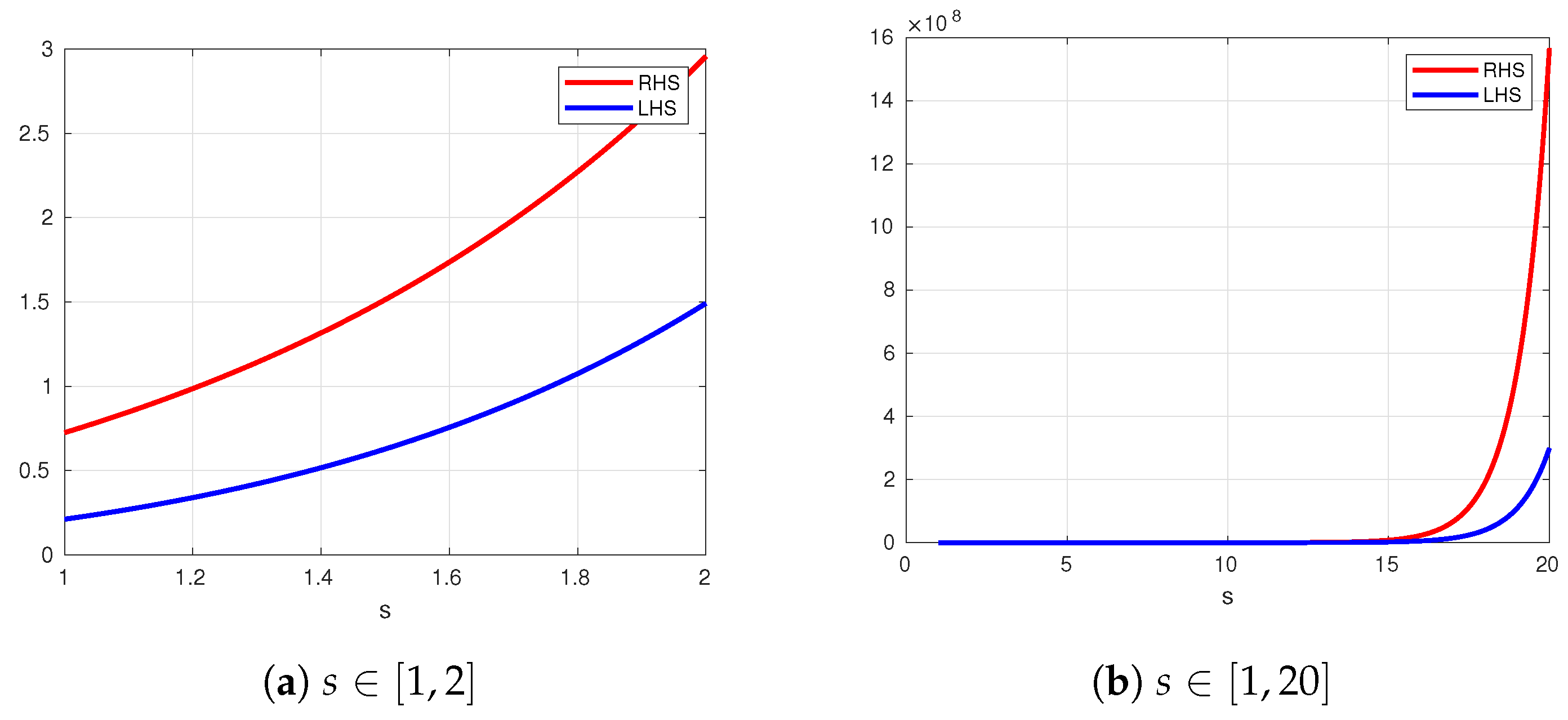
4. Graphical Illustration Example

In this section, we present a numerical example with graphical representations that validate the accuracy of the obtained results.

Let us start by presenting a proposition that will be useful for the following developments.

Proposition 1.

Let $s\in \mathbb{R}$. The function $\mathcal{L}\left(u\right)=u^s$ on $\left(0,+\infty \right)$ is $GA$-convex.

Proof. 

Clearly, we have

$$\mathcal{L}\left(x^t{y}^{1-t}\right)={\left(x^t{y}^{1-t}\right)}^s={\left(x^s\right)}^t{\left(y^s\right)}^{1-t}.$$

(12)

Since $t\in \left[0,1\right]$, Young’s inequality yields

$${\left(x^s\right)}^t{\left(y^s\right)}^{1-t}\le t{x}^s+\left(1-t\right)y^s.$$

(13)

Combing (12) and (13), we obtain

$$\mathcal{L}\left(x^t{y}^{1-t}\right)\le t{x}^s+\left(1-t\right)y^s=t\mathcal{L}\left(x\right)+\left(1-t\right)\mathcal{L}\left(y\right),$$

which is the desired result. □

Example 1.

Consider the function $\mathcal{L}$ defined on the interval $[k_1,k_2]$ by $\mathcal{L}\left(u\right)=u^s$. This function is $GA$ convex for $s\in \mathbb{R}$. According to Corollary 1, we have:

$$\begin{array}{}& & \frac{1}{3}\left(2{\left(k_1\right)}^s-{\left(k_1{k}_2\right)}^{{\displaystyle \frac{s}{2}}}+2{\left(k_2\right)}^s\right)-\frac{{\left(k_2\right)}^s-{\left(k_1\right)}^s}{s\left(ln{k}_2-ln{k}_1\right)}\hfill & \hfill \le & \frac{s}{{\left(ln{k}_2-ln{k}_1\right)}^2}\left(\left(4\sqrt{k_1{k}_2}-2k_2-2k_1+\frac{2k_2-5k_1+3\sqrt{k_1{k}_2}}{3}ln\frac{k_2}{k_1}-\frac{2k_1}{3}{\left(ln\frac{k_2}{k_1}\right)}^2\right){\left(k_1\right)}^{s-1}\right.\hfill \mathrm{(14)}& & +\left.\left(2k_2+2k_1-2\sqrt{k_1{k}_2}+\frac{3\sqrt{k_1{k}_2}-5k_2+2k_1}{3}ln\frac{k_2}{k_1}+\frac{2k_2-6\sqrt{k_1{k}_2}}{3}{\left(ln\frac{k_2}{k_1}\right)}^2\right){\left(k_2\right)}^{s-1}\right).\hfill \end{array}$$

The above result is illustrated in Figure 1 for $k_1=1$ and $k_2=e$, where $LHS$ denotes the left-hand side and $RHS$ denotes the right-hand side of inequality (14).

According to the representations given in Figure 1, the right-hand side is always above the left-hand side, thereby confirming the correctness of our results.

5. Application

This section presents some applications of the obtained results.

We recall the following means of real numbers.

• The arithmetic mean $A\left(k_1,k_2\right)={\displaystyle \frac{k_1+k_2}{2}}.$
• The geometric mean $G\left(k_1,k_2\right)=\sqrt{k_1{k}_2}$, where $k_1,k_2\ge 0.$
• The harmonic mean $H\left(k_1,k_2\right)={\displaystyle \frac{2k_1{k}_2}{k_1+k_2}}.$
• The logarithmic mean $L\left(k_1,k_2\right)={\displaystyle \frac{k_2-k_1}{ln{k}_2-ln{k}_1}}$, where $k_1,k_2>0$ with $k_1\ne k_2.$

Proposition 2.

For $0<k_1<k_2$, we have

$$\begin{array}{cc}\hfill & \left|4A\left(k_1^3,k_2^3\right)-G^3\left(k_1,k_2\right)-\left(2A\left(k_1^2,k_2^2\right)+G\left(k_1,k_2\right)\right)L\left(k_1,k_2\right)\right|\hfill \\ \hfill \le & \frac{9}{{\left(ln{k}_2-ln{k}_1\right)}^2}\left(\left(4\sqrt{k_1{k}_2}-2k_2-2k_1+\frac{2k_2-5k_1+3\sqrt{k_1{k}_2}}{3}ln\frac{k_2}{k_1}-\frac{2k_1}{3}{\left(ln\frac{k_2}{k_1}\right)}^2\right){\left(k_1\right)}^2\right.\hfill \\ \hfill & +\left.\left(2k_2+2k_1-2\sqrt{k_1{k}_2}+\frac{3\sqrt{k_1{k}_2}-5k_2+2k_1}{3}ln\frac{k_2}{k_1}+\frac{2k_2-6\sqrt{k_1{k}_2}}{3}{\left(ln\frac{k_2}{k_1}\right)}^2\right){\left(k_2\right)}^2\right).\hfill \end{array}$$

Proof. 

It suffices to apply Corollary 1 to the function $\mathcal{L}\left(u\right)=u^3$. □

Proposition 3.

For $0<k_1<k_2$, and $p,q>1$ with ${\displaystyle \frac{1}{p}}+{\displaystyle \frac{1}{q}}=1$, we have

$$\begin{array}{cc}\hfill & \left|4H^{-1}\left(k_1,k_2\right)-G^{-1}\left(k_1,k_2\right)-3G^{-2}\left(k_1,k_2\right)L\left(k_1,k_2\right)\right|\hfill \\ \hfill \le & \frac{3\left(ln{k}_2-ln{k}_1\right)}{4}\left({\left(\frac{2^{p+1}{\left(k_2{k}_1\right)}^{\frac{p}{2}}\gamma \left(p+1,\frac{p}{2}ln\left(\frac{k_2}{k_1}\right)\right)}{p^{p+1}{\left(ln{k}_2-ln{k}_1\right)}^{p+1}}+\frac{2k_2^{\frac{p}{2}}}{3^{p}p}\frac{k_2^{\frac{p}{2}}-k_1^{\frac{p}{2}}}{\left(ln{k}_2-ln{k}_1\right)}\right)}^{{\displaystyle \frac{1}{p}}}{\left(\frac{k_2^q+3k_1^q}{4k_1^q{k}_2^q}\right)}^{{\displaystyle \frac{1}{q}}}\right.\hfill \\ \hfill & +\left.{\left(\frac{k_2^p}{3^p}+\frac{2^{p+1}{\left(k_2{k}_1\right)}^{\frac{p}{2}}}{p^{p+1}{\left(ln{k}_2-ln{k}_1\right)}^{p+1}}\gamma \left(p+1,\frac{p}{2}ln\left(\frac{k_2}{k_1}\right)\right)\right)}^{{\displaystyle \frac{1}{p}}}{\left(\frac{3k_2^q+k_1^q}{4k_1^q{k}_2^q}\right)}^{{\displaystyle \frac{1}{q}}}\right).\hfill \end{array}$$

Proof. 

It suffices to apply Corollary 2 to the function $\mathcal{L}\left(u\right)={\displaystyle \frac{1}{u}}$. □

6. Conclusions

In this work, we have established the limits on the error estimates of the Milne rule in the framework of Hadamard fractional-integral operators, which have shown significance and effectiveness in several areas of applied sciences. After introducing a new integral identity, we establish some fractional Milne-type inequalities for functions with $GA$-convex derivatives. The findings of this study could prompt further investigation into this fascinating subject. We also plan to study other quadrature formulas in this context to establish extensions to other forms of generalized convexity, weighted formulas, and higher dimensions.

References

1. Sadek, L.; Baleanu, D.; Abdo, M.S.; Shatanawi, W. Introducing novel θ-fractional operators: Advances in fractional calculus. J. King Saud-Univ.-Sci. 2024, 36, 103352. [Google Scholar] [CrossRef]
2. Kilbas, A.A.; Srivastava, H.M.; Trujillo, J.J. Theory and Applications of Fractional Differential Equations; North-Holland Mathematics Studies, 204; Elsevier Science B.V.: Amsterdam, The Netherlands, 2006. [Google Scholar]
3. Samko, S.G.; Kilbas, A.A.; Marichev, O.I. Fractional Integrals and Derivatives. Theory and Applications; Edited and with a Foreword by S. M. Nikol’skiĭ. Translated from the 1987 Russian Original. Revised by the Authors; Gordon and Breach Science Publishers: Yverdon, Switzerland, 1993. [Google Scholar]
4. Sadek, L.; Algefary, A. Extended Hermite–Hadamard inequalities. AIMS Math. 2024, 9, 36031–36046. [Google Scholar] [CrossRef]
5. Katugampola, U.N. New approach to a generalized fractional integral. Appl. Math. Comput. 2011, 218, 860–865. [Google Scholar] [CrossRef]
6. Alraqad, T.; Almalahi, M.A.; Mohammed, N.; Alahmade, A.; Aldwoah, K.A.; Saber, H. Modeling Ebola Dynamics with a Φ-Piecewise Hybrid Fractional Derivative Approach. Fractal Fract. 2024, 8, 596. [Google Scholar] [CrossRef]
7. Hamza, A.; Osman, O.; Ali, A.; Alsulami, A.; Aldwoah, K.; Mustafa, A.; Saber, H. Fractal-Fractional-Order Modeling of Liver Fibrosis Disease and Its Mathematical Results with Subinterval Transitions. Fractal Fract. 2024, 8, 638. [Google Scholar] [CrossRef]
8. Saber, H.; Imsatfia, M.; Boulares, H.; Moumen, A.; Alraqad, T. On the Existence and Ulam Stability of BVP within Kernel Fractional Time. Fractal Fract. 2023, 7, 852. [Google Scholar] [CrossRef]
9. Nassima, N.; Meftah, B.; Moumen, A.; Saber, H. Fractional 3/8-Simpson type inequalities for differentiable convex functions. AIMS Math. 2024, 9, 5349–5375. [Google Scholar]
10. Saber, H.; Almalahi, M.A.; Albala, H.; Aldwoah, K.; Alsulami, A.; Shah, K.; Moumen, A. Investigating a Nonlinear Fractional Evolution Control Model Using W-Piecewise Hybrid Derivatives: An Application of a Breast Cancer Model. Fractal Fract. 2024, 8, 735. [Google Scholar] [CrossRef]
11. Sadek, L. A cotangent fractional derivative with the application. Fractal Fract. 2023, 7, 444. [Google Scholar] [CrossRef]
12. Fallahgoul, H.A.; Focardi, S.M.; Fabozzi, F.J. Fractional Calculus and Fractional Processes with Applications to Financial Economics; Theory and Application; Elsevier/Academic Press: London, UK, 2017. [Google Scholar]
13. Ruszczyński, A.; Shapiro, A. Optimization of convex risk functions. Math. Oper. Res. 2006, 31, 433–452. [Google Scholar] [CrossRef]
14. Pham, H. Continuous-Time Stochastic Control and Optimization with Financial Applications; Stochastic Modelling and Applied Probability, 61; Springer: Berlin/Heidelberg, Germany, 2009. [Google Scholar]
15. Carr, P.; Zhu, Q.J. Convex Duality and Financial Mathematics; SpringerBriefs in Mathematics; Springer: Cham, Switzerland, 2018. [Google Scholar]
16. Bertsekas, D.P. Convex Optimization Theory; Athena Scientific: Nashua, NH, USA, 2009. [Google Scholar]
17. Cambini, A.; Martein, L. Generalized Convexity and Optimization; Theory and Applications; With a Foreword by Siegfried Schaible; Lecture Notes in Economics and Mathematical Systems, 616; Springer: Berlin/Heidelberg, Germany, 2009. [Google Scholar]
18. Owen, G. Game Theory, 4th ed.; Emerald Group Publishing Limited: Bingley, UK, 2013. [Google Scholar]
19. Alomari, M.W.; Dragomir, S.S. Various error estimations for several Newton-Cotes quadrature formulae in terms of at most first derivative and applications in numerical integration. Jordan J. Math. Stat. 2014, 7, 89–108. [Google Scholar]
20. Deng, J.; Wang, J. Fractional Hermite-Hadamard inequalities for (α,m)-logarithmically convex functions. J. Inequal. Appl. 2013, 364, 11. [Google Scholar] [CrossRef]
21. Dragomir, S.S.; Agarwal, R.P.; Cerone, P. On Simpson’s inequality and applications. J. Inequal. Appl. 2000, 5, 533–579. [Google Scholar] [CrossRef]
22. Meftah, B.; Benssaad, M.; Kaidouchi, W.; Ghomrani, S. Conformable fractional Hermite-Hadamard type inequalities for product of two harmonic s-convex functions. Proc. Amer. Math. Soc. 2021, 149, 1495–1506. [Google Scholar] [CrossRef]
23. Booth, A.D. Numerical Methods, 3rd ed.; Butterworths: La Canada Flintrige, CA, USA, 1966. [Google Scholar]
24. Alomari, M.; Liu, Z. New error estimations for the Milne’s quadrature formula in terms of at most first derivatives. Konuralp J. Math. 2013, 1, 17–23. [Google Scholar]
25. Djenaoui, M.; Meftah, B. Milne-type inequalities for differentiable s-convex functions. Honam Math. J. 2022, 44, 325–338. [Google Scholar]
26. Özarslan, M.A.; Ustaoğlu, C. Some incomplete hypergeometric functions and incomplete Riemann-πLiouville fractional integral operators. Mathematics 2019, 7, 483. [Google Scholar] [CrossRef]
27. Budak, H.; Kösem, P.; Kara, H. On new Milne-type inequalities for fractional integrals. J. Inequal. Appl. 2023, 10, 15. [Google Scholar] [CrossRef]
28. Meftah, B.; Lakhdari, A.; Saleh, W.; Kiliçman, A. Some new fractal Milne-type integral inequalities via generalized convexity with applications. Fractal Fract. 2023, 7, 166. [Google Scholar] [CrossRef]
29. Al-Sa’di, S.; Bibi, M.; Seol, Y.; Muddassar, M. Milne-type fractal integral inequalities for generalized m-convex mapping. Fractals 2023, 31, 2350081. [Google Scholar] [CrossRef]
30. Sial, I.B.; Budak, H.; Ali, M.A. Some Milne’s rule type inequalities in quantum calculus. Filomat 2023, 37, 9119–9134. [Google Scholar] [CrossRef]
31. Lakhdari, A.; Budak, H.; Mlaiki, N.; Meftah, B.; Abdeljawad, T. New insights on fractal–fractional integral inequalities: Hermite–Hadamard and Milne estimates. Chaos Solitons Fractals 2025, 193, 116087. [Google Scholar] [CrossRef]
32. Bin-Mohsin, B.; Javed, M.Z.; Awan, M.U.; Khan, A.G.; Noor, C.C.M.A. Exploration of Quantum Milne–Mercer-Type Inequalities with Applications. Symmetry 2023, 15, 1096. [Google Scholar] [CrossRef]
33. Bosch, P.; Rodríguez, J.M.; Sigarreta, J.M. On new Milne-type inequalities and applications. J. Inequal. Appl. 2023, 3, 18. [Google Scholar] [CrossRef]
34. Budak, H.; Hyder, A.A. Enhanced bounds for Riemann-Liouville fractional integrals: Novel variations of Milne inequalities. AIMS Math. 2023, 8, 30760–30776. [Google Scholar] [CrossRef]
35. Budak, H.; Karagözoğlu, P. Fractional Milne-type inequalities. Acta Math. Univ. Comen. 2024, 93, 1–15. [Google Scholar]
36. Demir, I. A new approach of Milne-type inequalities based on proportional Caputo-Hybrid operator: A new approach for Milne-type inequalities. J. Adv. App. Comput. 2023, 10, 102–119. [Google Scholar] [CrossRef]
37. Desta, H.D.; Budak, H.; Kara, H. New perspectives on fractional Milne-type inequalities: Insights from twice-differentiable functions. Univers. J. Math. Appl. 2024, 7, 30–37. [Google Scholar] [CrossRef]
38. Shehzadi, A.; Budak, H.; Haider, W.; Chen, H. Milne-type inequalities for co-ordinated convex functions. Filomat 2024, 38, 8295–8303. [Google Scholar]
39. Munir, A.; Qayyum, A.; Rathour, L.; Atta, G.; Supadi, S.S.; Ali, U. A study on Milne-type inequalities for a specific fractional integral operator with applications. Korean J. Math. 2024, 32, 297–314. [Google Scholar]
40. Hezenci, F.; Budak, H.; Kara, H.; Baş, U. Novel results of Milne-type inequalities involving tempered fractional integrals. Bound. Value Probl. 2024, 12, 15. [Google Scholar] [CrossRef]
41. Niculescu, C.P. Convexity according to the geometric mean. Math. Inequal. Appl. 2000, 3, 155–167. [Google Scholar] [CrossRef]
42. İşcan, İ. New general integral inequalities for quasi-geometrically convex functions via fractional integrals. J. Inequal. Appl. 2013, 491, 15. [Google Scholar] [CrossRef]
43. Chiheb, T.; Meftah, B.; Moumen, A.; Bouye, M. Maclaurin type integral inequalities for GA-convex functions involving confluent hypergeometric function via Hadamard fractional integrals. Fractal Fract. 2023, 7, 860. [Google Scholar] [CrossRef]
44. İşcan, İ. Hermite-Hadamard and Simpson type inequalities for differentiable P-GA-functions. Int. J. Anal. 2014, 2014, 125439. [Google Scholar] [CrossRef]
45. İşcan, İ.; Aydin, M. Some new generalized integral inequalities for GA-s-convex functions via Hadamard fractional integrals. Chin. J. Math. 2016, 2016, 4361806. [Google Scholar] [CrossRef]
46. Kalsoom, H.; Latif, M.A. Some weighted Hadamard and Ostrowski-type fractional inequalities for quasi-geometrically convex functions. Filomat 2023, 37, 5921–5942. [Google Scholar] [CrossRef]
47. Latif, M.A. Some Companions of Fejér Type Inequalities Using GA-Convex Functions. Mathematics 2023, 11, 392. [Google Scholar] [CrossRef]
48. Latif, M.A. Extensions of Fejér type inequalities for GA-convex functions and related results. Filomat 2023, 37, 8041–8055. [Google Scholar] [CrossRef]
49. Latif, M.A. Properties of GA-h-Convex Functions in Connection to the Hermite–Hadamard–Fejér-Type Inequalities. Mathematics 2023, 11, 3172. [Google Scholar] [CrossRef]
50. Jameson, G.J.O. The incomplete gamma functions. Math. Gaz. 2016, 100, 298–306. [Google Scholar] [CrossRef]
51. Park, J. Some Hermite-Hadamard-like type inequalities for logarithmically convex functions. Int. J. Math. Anal. 2013, 7, 2217–2233. [Google Scholar] [CrossRef]
Figure 1. Illustration of inequality (14).
Fractalfract 09 00129 g001
Disclaimer/Publisher’s Note: The statements, opinions and data contained in all publications are solely those of the individual author(s) and contributor(s) and not of MDPI and/or the editor(s). MDPI and/or the editor(s) disclaim responsibility for any injury to people or property resulting from any ideas, methods, instructions or products referred to in the content.