
Research on Nonlinear Dynamic Characteristics of Fractional Order Resonant DC-DC Converter Based on Sigmoid Function

Abstract
1. Introduction
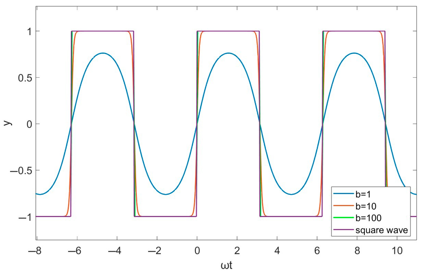
2. Sigmoid Function
3. Sigmoid Function Model of FO Resonant DC-DC Converter
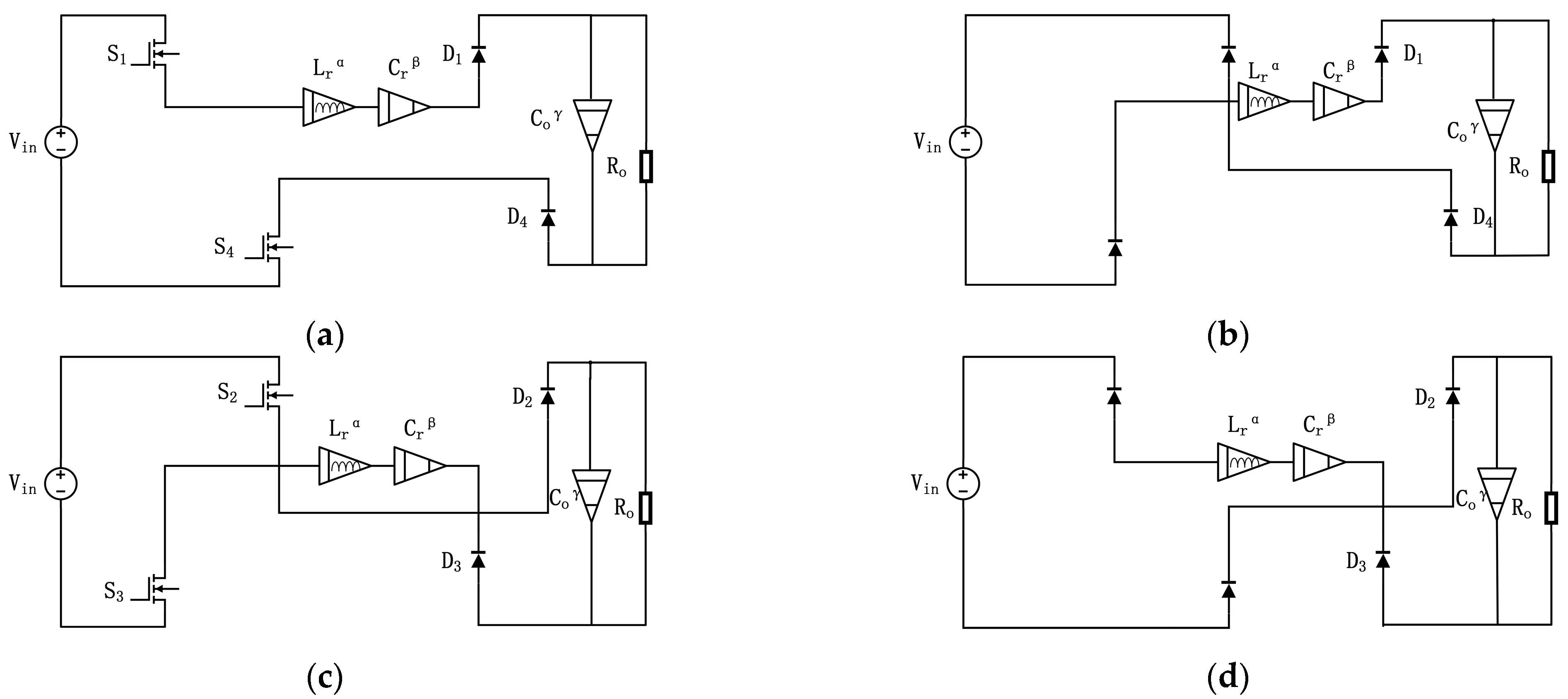
3.1. Mathematical Modeling
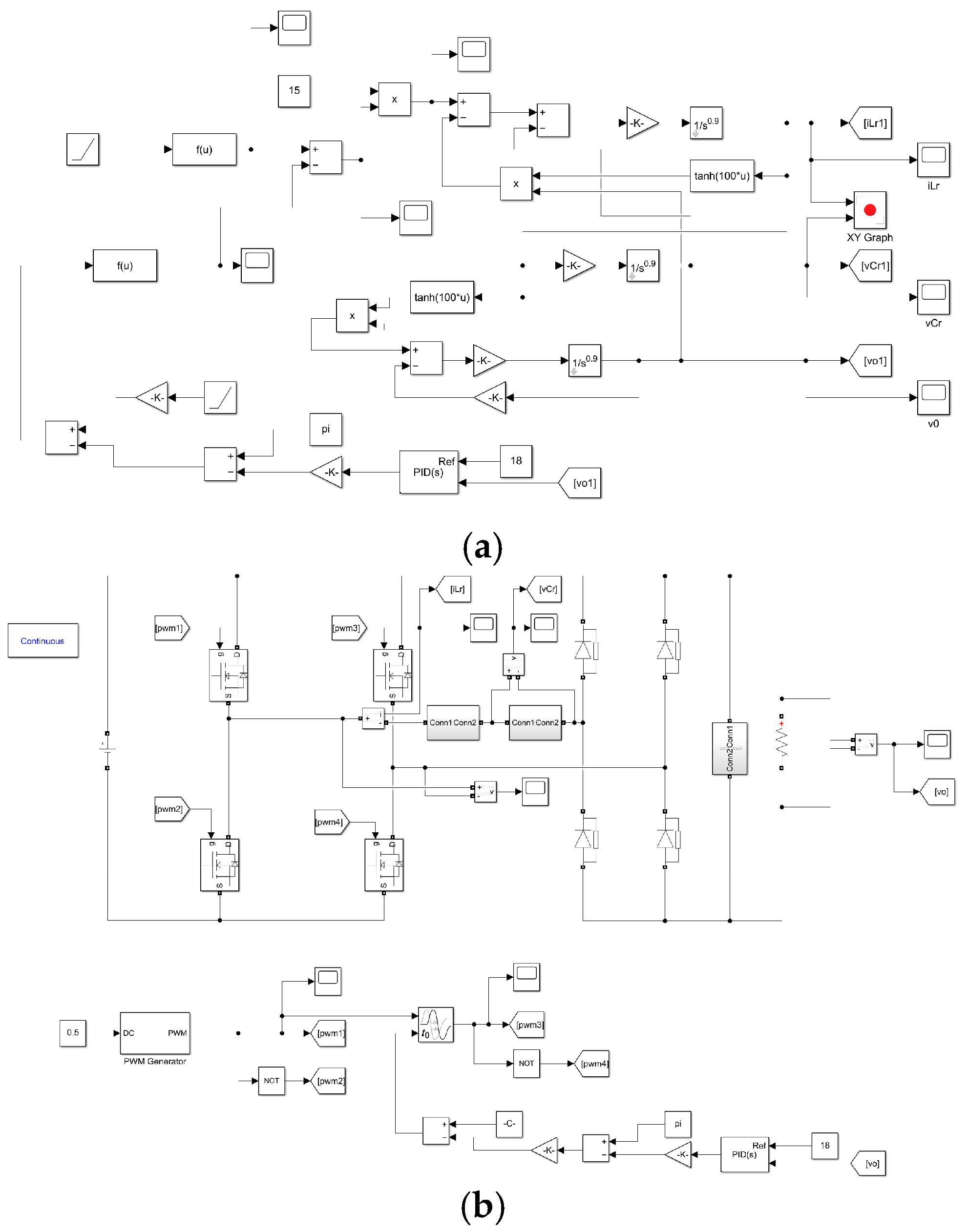
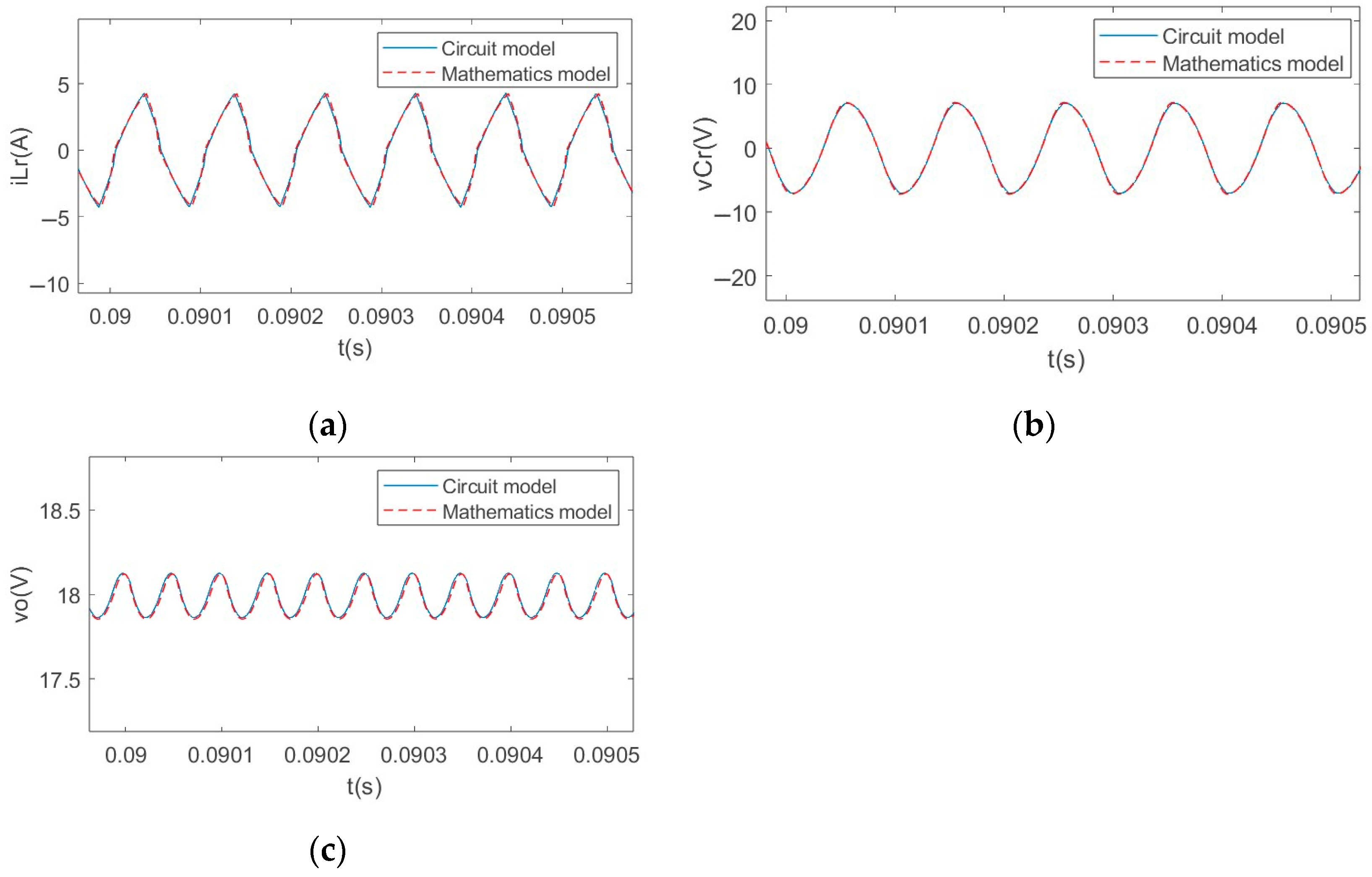
3.2. Simulation
4. Dynamics Behavior and Stability Analysis
4.1. FO Estimation Correction Algorithm
4.2. Discrete Mathematical Model Based on Sigmoid Function Mathematical Model
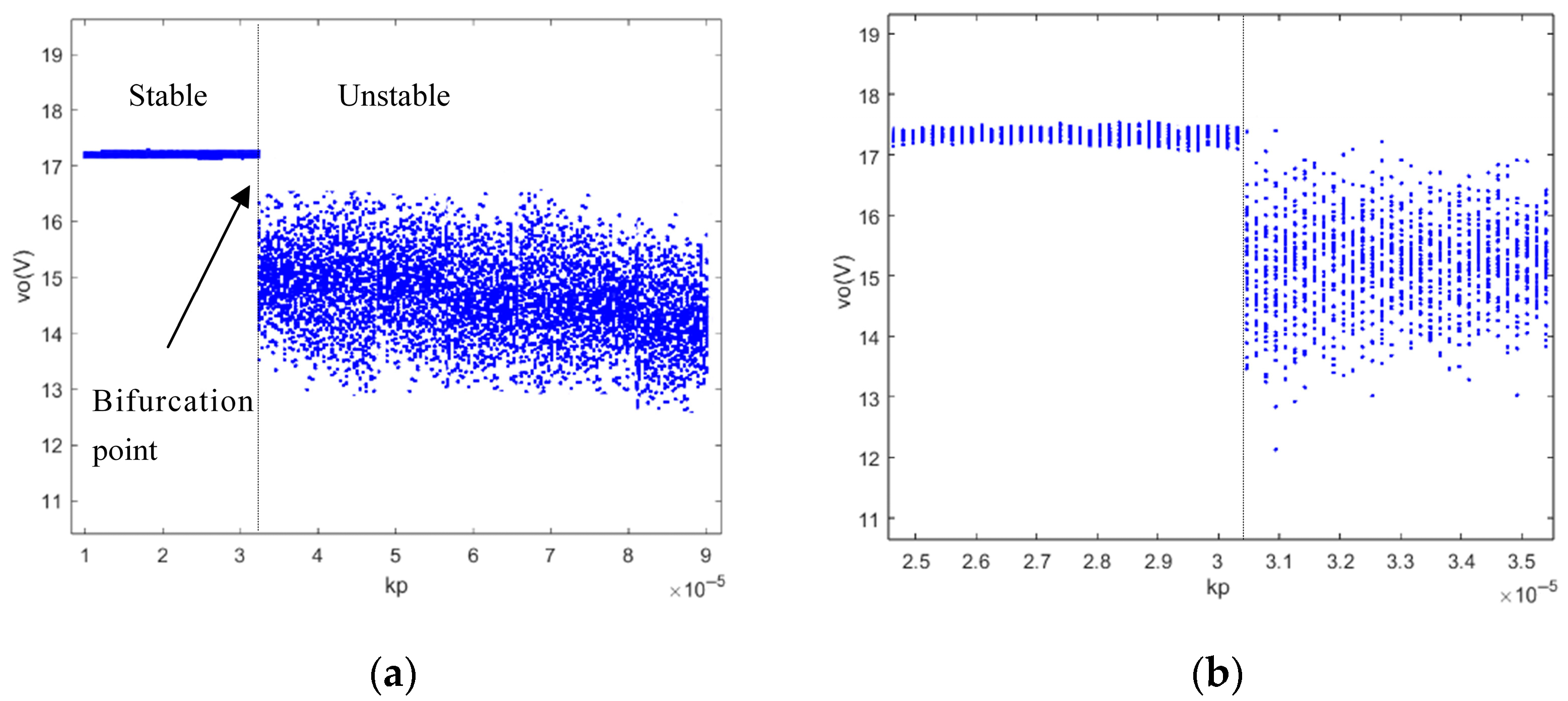
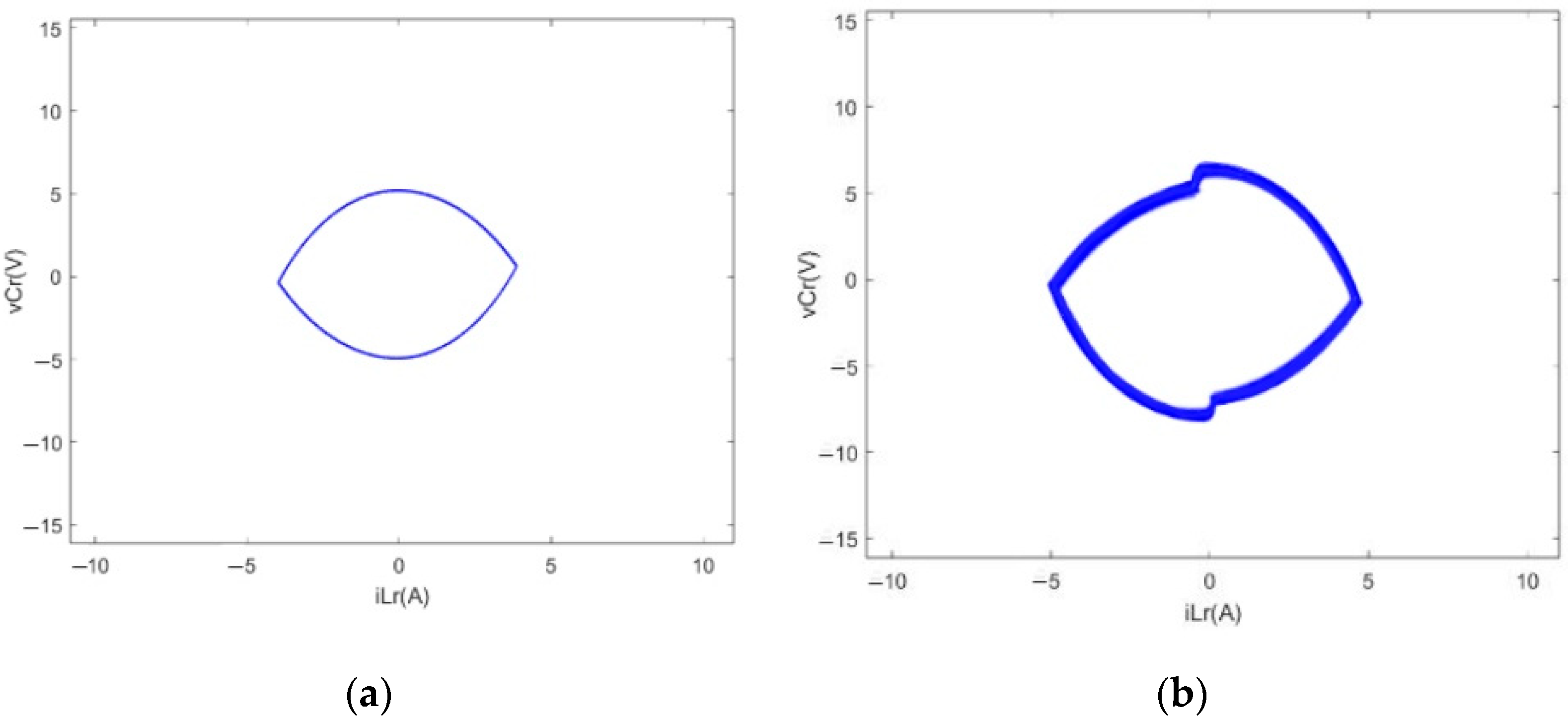
4.3. Proportional Coefficient kp as Bifurcation Parameter
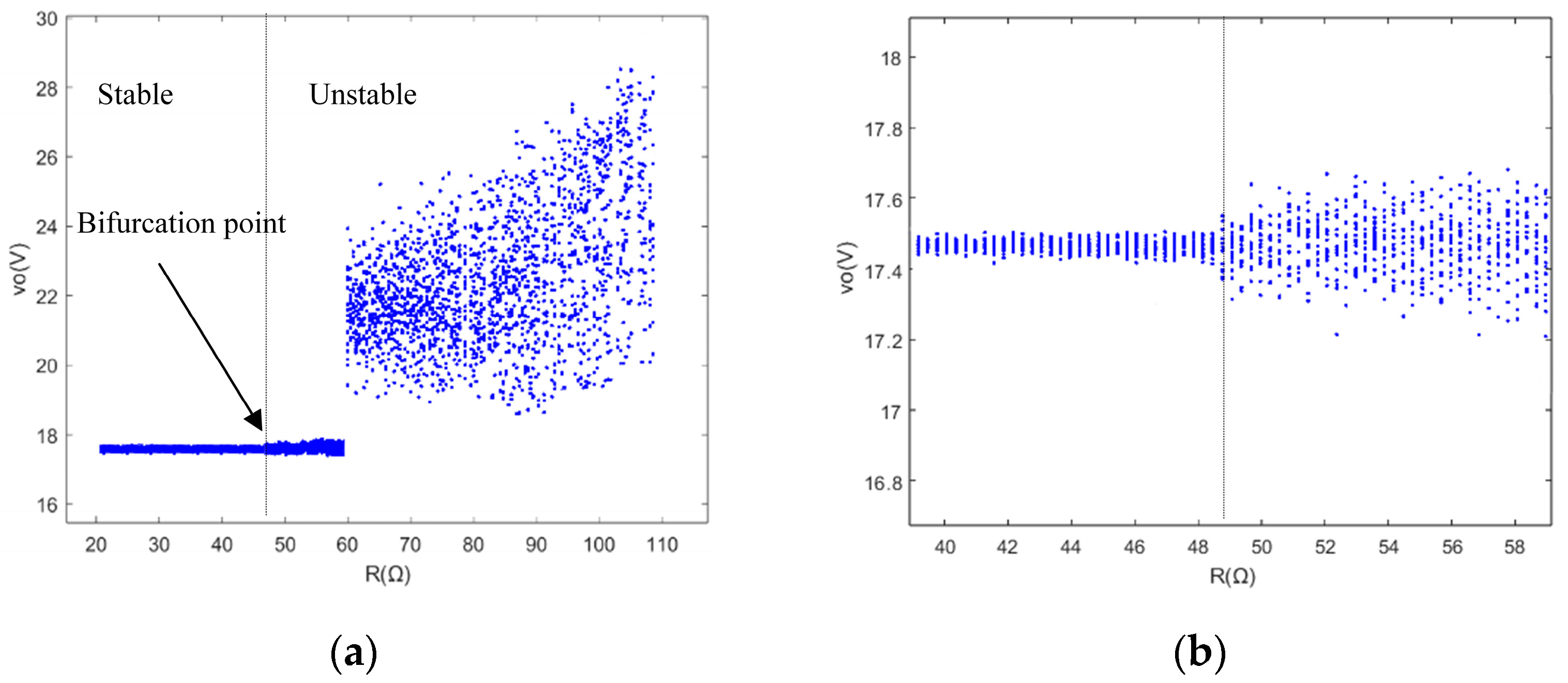
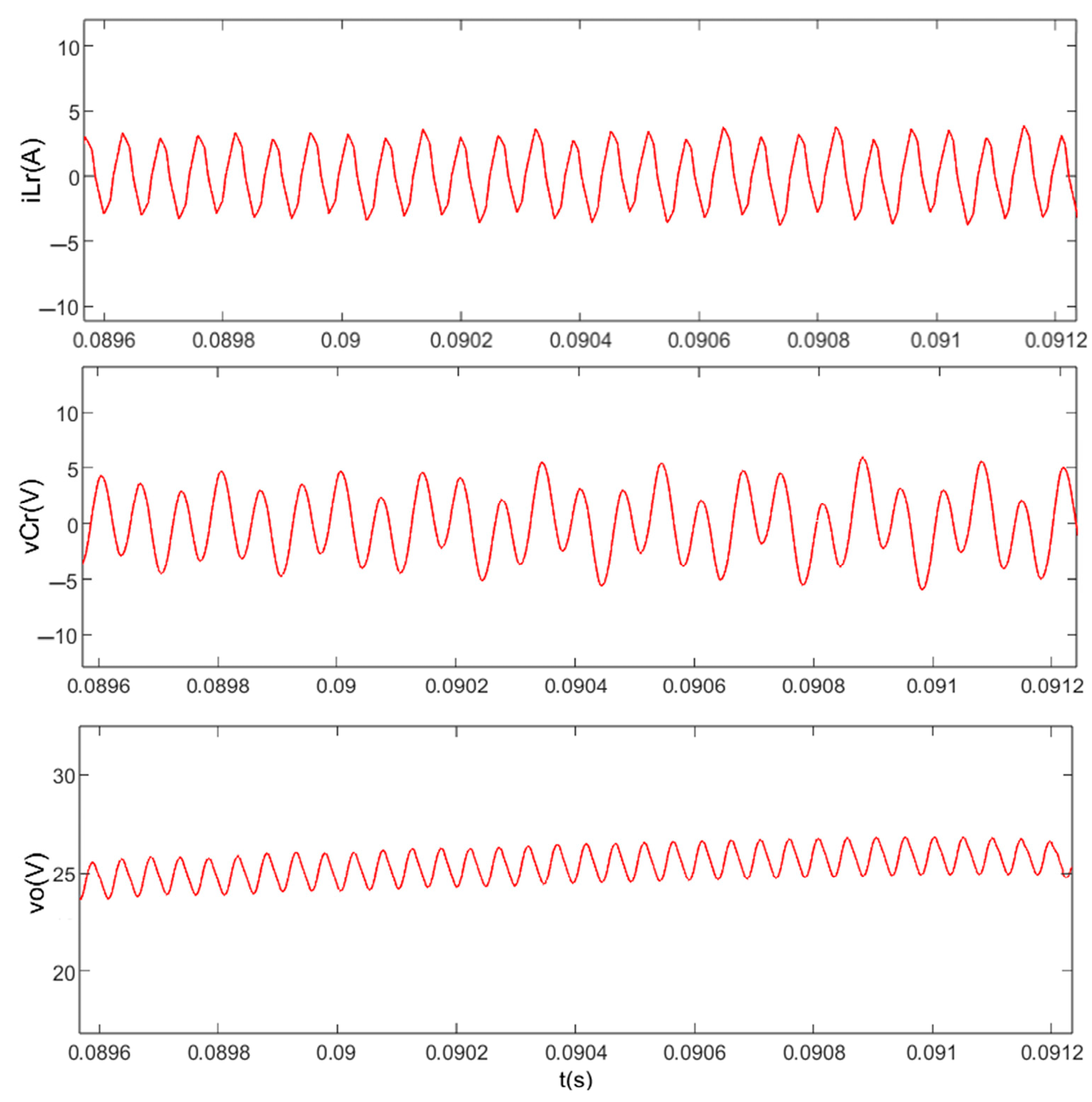
4.4. Load Resistance R as Bifurcation Parameter
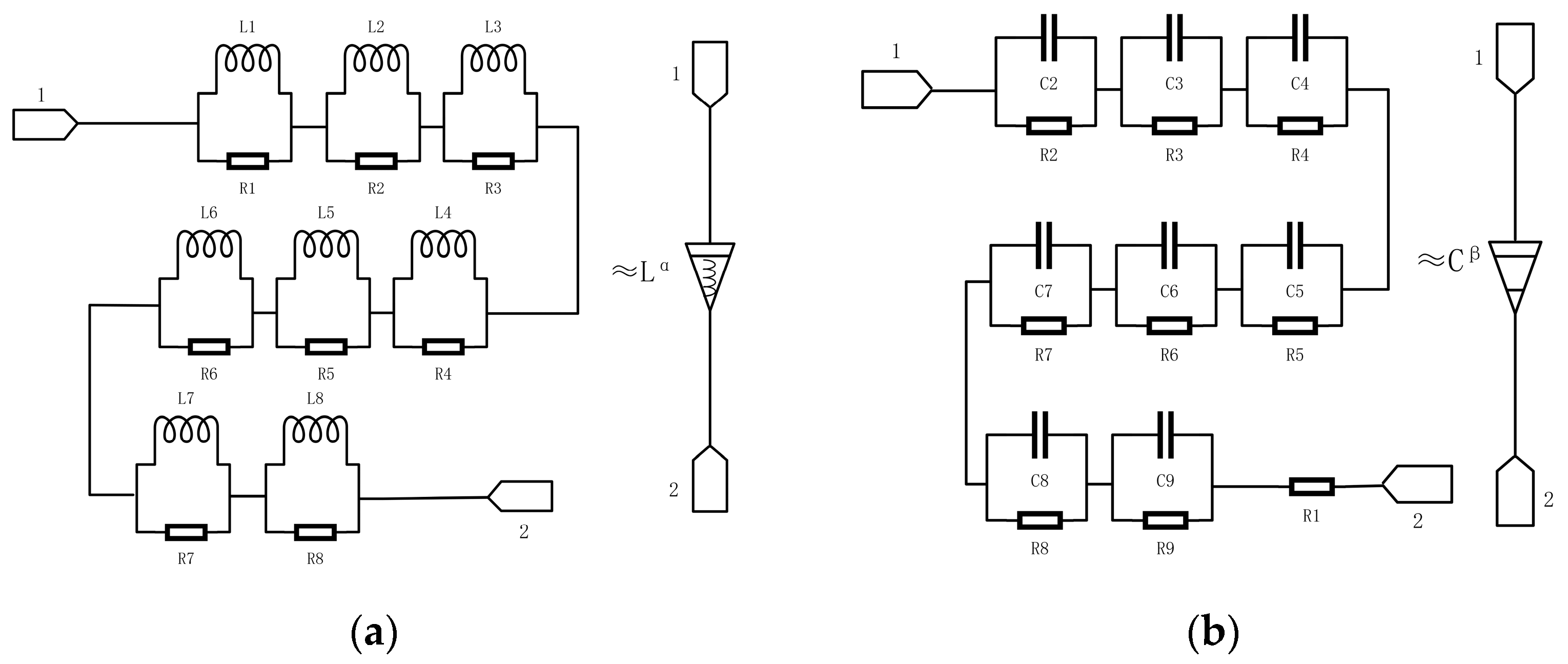
4.5. Fractional Order of Inductance and Capacitance as Bifurcation Parameter
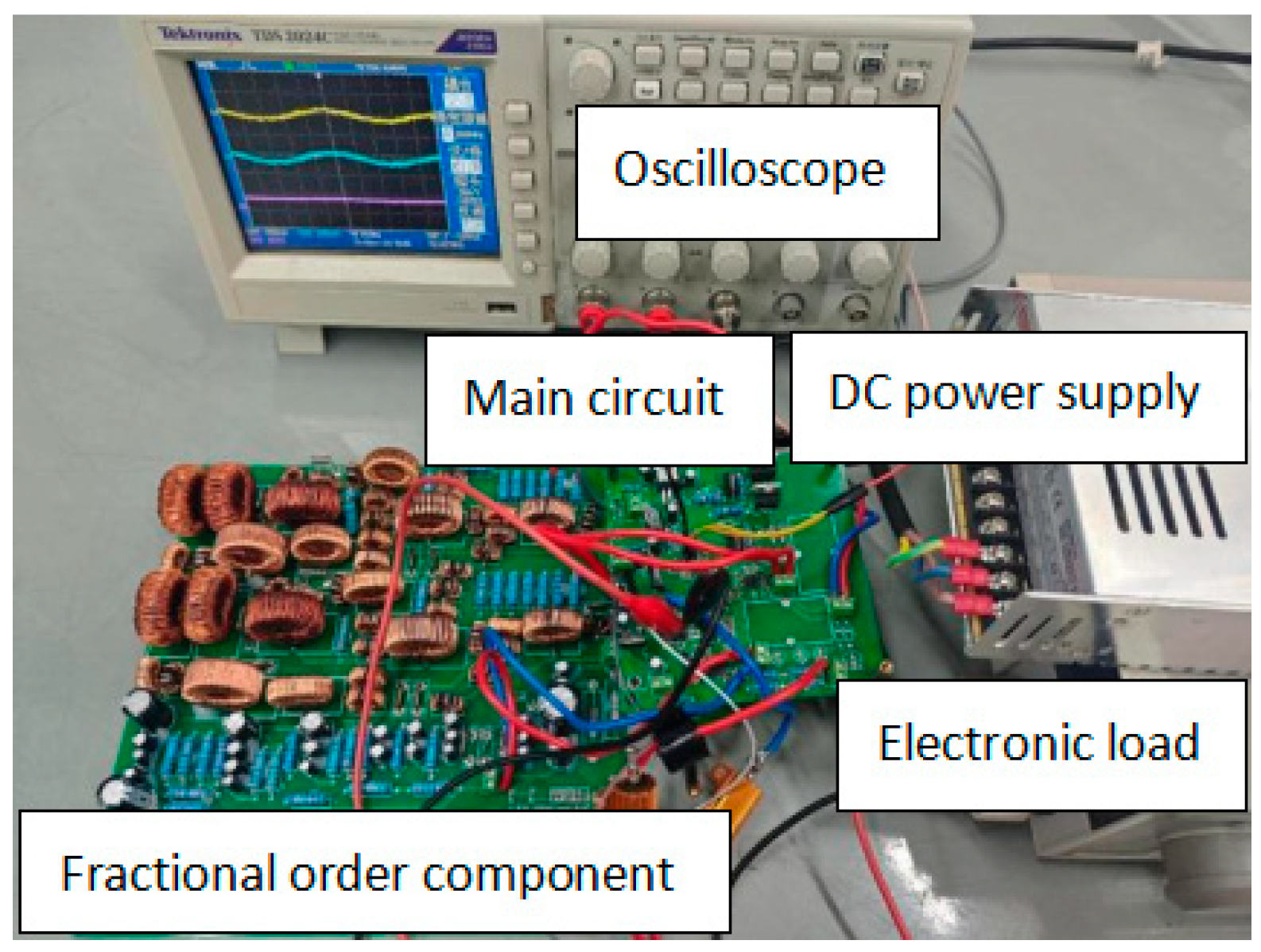
5. Experiments
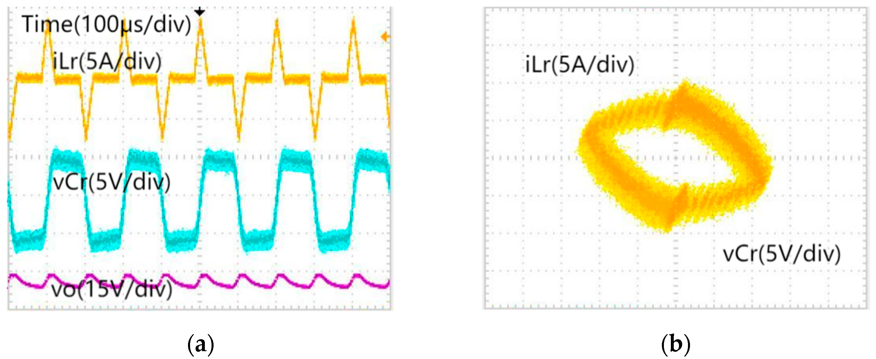
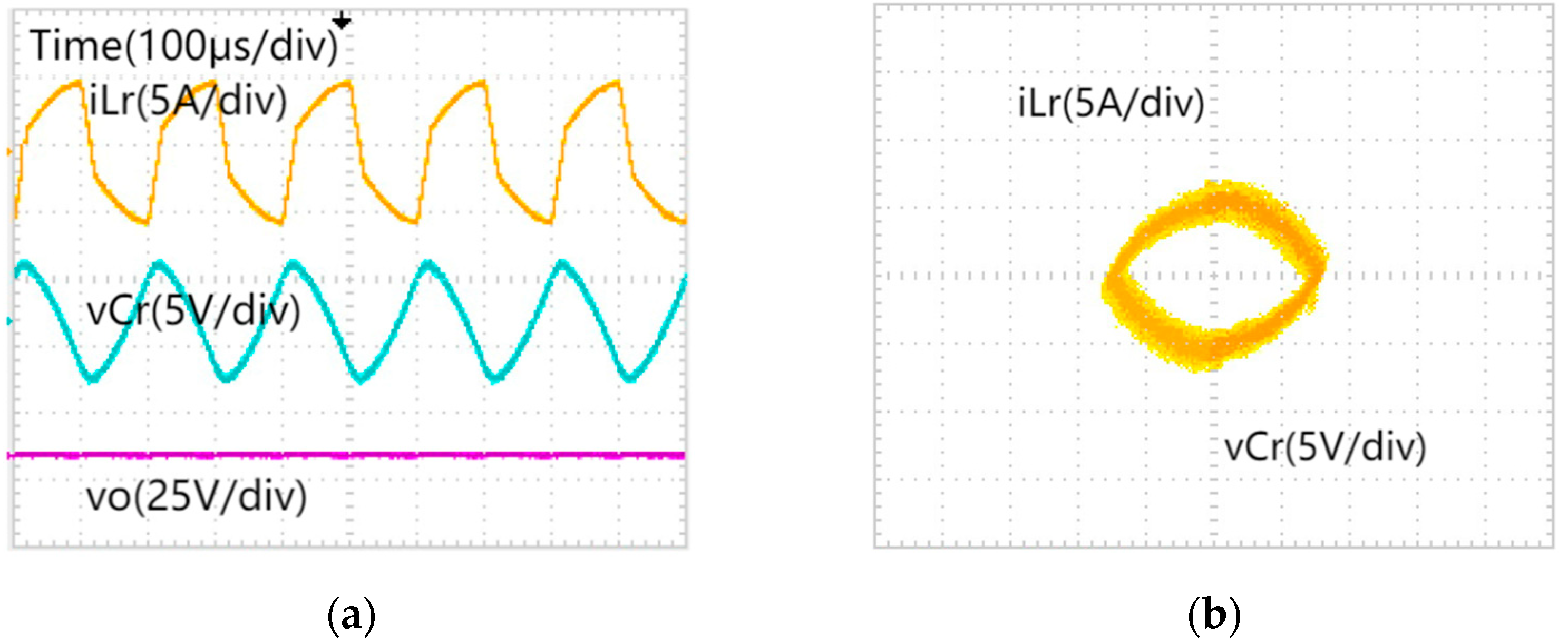
5.1. The Effect of Proportional Coefficient kp on System Dynamics Behavior
5.2. The Effect of Load R on System Dynamics Behavior
6. Conclusions
Author Contributions
Funding
Data Availability Statement
Conflicts of Interest
Abbreviations
| FO | Fractional order; |
| IO | Integer order; |
| Lr | Resonant inductor; |
| Cr | Resonant capacitor; |
| Vin | Input voltage; |
| f | Switching frequency; |
| R | Load; |
| Vref | Reference voltage; |
| kp | Proportional coefficient; |
| ki | Integral coefficient; |
| α | Inductance order; |
| β, γ | Capacitance order. |
References
- Chang, C.H.; Chang, E.C.; Cheng, H.L. A high-efficiency solar array simulator implemented by an LLC resonant DC-DC converter. J. IEEE Trans. Power Electron. 2013, 28, 3039–3046. [Google Scholar] [CrossRef]
- Feng, J.; Li, Q.; Lee, F.C. LCCL-LC resonant converter and its soft switching realization for omnidirectional wireless power transfer systems. J. IEEE Trans. Power Electron. 2021, 36, 3828–3839. [Google Scholar] [CrossRef]
- Mi, C.C.; Buja, G.; Choi, S.Y. Modern advances in wireless power transfer systems for roadway powered electric vehicles. J. IEEE Trans. Ind. Electron. 2016, 63, 6533–6545. [Google Scholar] [CrossRef]
- Zhang, X.; Ma, X.; Zhang, H. Low-frequency oscillation in digitally controlled DC-DC Buck converters. J. Acta Phys. Sin. 2008, 57, 6174–6181. [Google Scholar] [CrossRef]
- Wang, X.; Zhang, B.; Qiu, D. Mechanism of period-doubling bifurcation in DCM DC-DC converter. J. Acta Phys. Sin. 2008, 57, 2728–2736. [Google Scholar] [CrossRef]
- Gan, H. Stabilization and Dynamical Analysis of V2 Controlled Boost Converter. Ph.D. Thesis, Southwest Jiaotong University, Chengdu, China, 2019. [Google Scholar]
- Tse, C.K. Flip bifurcation and chaos in a three-state boost switching regulator. J. IEEE Trans. Circuits Syst. I Fundam. Theory Appl. 1994, 41, 16–23. [Google Scholar] [CrossRef]
- Li, Z.; Li, Y.; Wu, C. Study on bifurcation behaviors and stabilization in current mode controlled Buck converter. J. Power Syst. Prot. Control 2016, 44, 544–560. [Google Scholar]
- Li, H.; Zhou, Y.F.; Ling, Q.Q. Modeling and dynamics of Boost converter based on nonlinear inductor. J. Electr. Meas. Instrum. 2019, 56, 39–44. [Google Scholar]
- Sun, L.X.; Zhou, Z.Y.; Wen, Z.G. Adaptive carrier amplitude modulation control of bifurcation and chaos in SPWM H-bridge converter. J. Electr. Meas. 2020, 57, 101–108. [Google Scholar]
- Jesus, I.S.; Machado, J.A.T. Development of fractional order capacitors based on electrolyte processes. J. Nonlinear Dyn. 2009, 56, 45–55. [Google Scholar] [CrossRef]
- Westerlund, S. Dead matter has memory. J. Causal Consult. 2002, 244, 4–9. [Google Scholar] [CrossRef]
- Wei, X.; Yi, L.; Xin, G. Sigmoid Function Model and Dynamic Characteristics Analysis for Inductive Wireless Power Transmission Control System. J. IEEE Trans. Ind. Electron. 2022, 69, 11112–11120. [Google Scholar] [CrossRef]
- Sun, H.; Chen, W.; Sun, L. Fractional order simulation model and chaos analysis of Buck converter. J. Mod. Electron. Tech. 2014, 24, 154–159+162. [Google Scholar]
- Jia, Z.; Liu, C. Fractional-order modeling and simulation of magnetic coupled boost converter in continuous conduction mode. J. Int. J. Bifurc. Chaos 2018, 28, 1850061. [Google Scholar] [CrossRef]
- Liu, M. Study on Nonlinear Dynamics of Fractional Order Switching Converters. Ph.D. Thesis, University of Electronic Science and Technology of China, Chengdu, China, 2018. [Google Scholar]
- Cheng, L.; Bi, C.; He, J. Fractional Order Modeling and Dynamical Analysis of Peak-Current-Mode Controlled Synchronous Switching Z-Source Converter. In Proceedings of the 2021 4th Internation Conference on Energy, Electrical and Power Engineering (CEEPE), Chongqing, China, 23–25 April 2021; pp. 148–152. [Google Scholar]
- Jia, H. Research on Nonlinear Dynamics and Chaos Control of Fractional Buck Boost Converter. Ph.D. Thesis, Guangxi University, Nanning, China, 2022. [Google Scholar]
- Jia, Z.; Liu, C. A modified modeling and dynamical behavior analysis method for fractional-order positive Luo converter. PLoS ONE 2020, 15, e0237169. [Google Scholar] [CrossRef]
- Basterretxea, K.; Tarela, J.M.; Campo, I.D. Approximation of sigmoid function and the derivative for hardware implementation of artificial neurons. J. Circuits Devices Syst. 2004, 151, 18–24. [Google Scholar] [CrossRef]
- Westerlund, S.; Ekstam, L. Capacitor theory. J. IEEE Trans. Dielectr. Electr. Insul. 1994, 1, 826–839. [Google Scholar] [CrossRef]
- Kai, D.; Ford, N.J.; Freed, A.D. A predictor-corrector approach for the numerical solution of fractional differential equations. J. Nonlinear Dyn. 2002, 29, 3–22. [Google Scholar]
- Xue, D. Fractional Calculus and Fractional Order Control; Science Press: Beijing, China, 2018. [Google Scholar]


| Parameters | Values |
|---|---|
| Resonant inductor (Lr) | 1.19 × 10⁻⁴ |
| Resonant capacitor (Cr) | 8.49 × 10⁻⁶ |
| Input voltage (Vin) | 30 V |
| Switching frequency (f) | 10,000 Hz |
| Load (R) | 10 Ω |
| Reference voltage (Vref) | 18 V |
| Proportional coefficient (kp) | 2.5 × 10⁻⁵ |
| Integral coefficient (ki) | 2 × 10⁻³ |
| Inductance order (α) | 0.9 |
| Capacitance order (β) | 0.9 |
| L = 1.19 × 10⁻⁴ H | C = 8.49 × 10⁻⁶ F | |||
|---|---|---|---|---|
| α = 0.9 | β = 0.9 | |||
| i | RLi (Ω) | Li (H) | RCi (Ω) | Ci (F) |
| 1 | 229.920 k | 26.18 m | 190.091 | |
| 2 | 96.564 | 10.834 m | 169.8 m | 40.073 m |
| 3 | 190.4 m | 21.363 m | 130.058 | 52.332 m |
| 4 | 775.330 | 8.701 m | 100.326 k | 67.835 m |
| 5 | 1.528 | 17.112 m | 14.594 | 46.619 m |
| 6 | 6.624 k | 7.433 m | 10.475 k | 64.957 m |
| 7 | 12.207 | 13.428 m | 1.613 | 42.204 m |
| 8 | 21.960 m | 23.8 m | 1.162 k | 58.309 m |
| 9 | 7456.597 k | 9.127 m | ||
Disclaimer/Publisher’s Note: The statements, opinions and data contained in all publications are solely those of the individual author(s) and contributor(s) and not of MDPI and/or the editor(s). MDPI and/or the editor(s) disclaim responsibility for any injury to people or property resulting from any ideas, methods, instructions or products referred to in the content. |
© 2025 by the authors. Licensee MDPI, Basel, Switzerland. This article is an open access article distributed under the terms and conditions of the Creative Commons Attribution (CC BY) license (https://creativecommons.org/licenses/by/4.0/).
Share and Cite
Xie, L.; Xu, G. Research on Nonlinear Dynamic Characteristics of Fractional Order Resonant DC-DC Converter Based on Sigmoid Function. Fractal Fract. 2025, 9, 111. https://doi.org/10.3390/fractalfract9020111
Xie L, Xu G. Research on Nonlinear Dynamic Characteristics of Fractional Order Resonant DC-DC Converter Based on Sigmoid Function. Fractal and Fractional. 2025; 9(2):111. https://doi.org/10.3390/fractalfract9020111
Chicago/Turabian StyleXie, Lingling, and Guangwei Xu. 2025. "Research on Nonlinear Dynamic Characteristics of Fractional Order Resonant DC-DC Converter Based on Sigmoid Function" Fractal and Fractional 9, no. 2: 111. https://doi.org/10.3390/fractalfract9020111
APA StyleXie, L., & Xu, G. (2025). Research on Nonlinear Dynamic Characteristics of Fractional Order Resonant DC-DC Converter Based on Sigmoid Function. Fractal and Fractional, 9(2), 111. https://doi.org/10.3390/fractalfract9020111