A Note on Solutions of Fractional Third-Order Dispersive Partial Differential Equations Using the Natural Generalized Laplace Transform Decomposition Method

Abstract

The present research offers reliable analytical solutions for time-fractional linear and nonlinear dispersive Korteweg–de Vries (dKdV)-type equations by employing the Natural Generalized Laplace Transform Decomposition Method (NGLTDM). The nonlinear differential dispersive Korteweg–de Vries (dKdV) equation involves a nonlinear derivative term that depends on $\varphi$ and its partial derivative with respect to x. We employ Adomian polynomials to deal with this nonlinear part, and we utilize the Caputo derivative to illustrate the fractional part of the equation. The work provides exact theorems regarding the stability, convergence, and accuracy of the generated solutions. Illustrative examples demonstrate the effectiveness and precision of the method by delivering solutions for quickly converging series with easily calculable coefficients. We use Maple 2021 software to show graphical comparisons between the approximate and exact solutions to show how rapidly the method converges.

1. Introduction

Fractional calculus has gained considerable attention across various scientific and engineering disciplines due to its broad range of applications and its crucial role in describing the complex dynamic behavior of real-world phenomena such as biological populations, diffusion processes, fluid dynamics, and traffic systems. This mathematical framework demonstrates considerable effectiveness in the examination of wave phenomena observed in diverse scientific and technological areas.

Time-fractional third-order dispersive partial differential equations are very important in the area of mathematics, as they are essential for modeling complex dynamical systems and developing advanced analytical techniques. In [1], a combination of the Laplace Transform (LT) and the Adomian Decomposition Method (ADM) was employed to solve various forms of the (dKdV) equation. Authors in [2] investigated the KdV-Burgers equation with non-singular kernel operators using a modified double Laplace transform approach. The Fractional Differential Transform Method (FDTM) and its modified form (MFDTM) have also been used to derive solutions of fractional third-order dispersive partial differential equations in both one- and multi-dimensional domains [3].

A hybrid numerical scheme combining the Sumudu Transform and the Homotopy Analysis Method (HAM) was proposed in [4] for solving time-fractional third-order dispersive partial differential equations. The authors in [5] introduced a novel Fractional Shehu Transform Iterative Method (FSTIM) to handle nonlinear time-fractional hyperbolic partial differential equations (NTFHPDEs).

More recently, a comprehensive computational framework based on the conformable Laplace–Adomian decomposition method was introduced in [6] to address KdV models, demonstrating the efficiency of hybrid integral transform approaches in handling dispersive systems. The authors in [7] addressed third-order dispersive equations by applying a decomposition approach that combines the Sumudu and generalized Laplace transforms. Appadu and Kelil [8] utilized various semi-analytic techniques, including LADM, homotopy perturbation (HPM), and RDTM, while further developing the Bernstein ALDM to handle linearized dKdV equations with both homogeneous and inhomogeneous source terms.

The numerical behavior of third- and fifth-order dKdV equations was analyzed in [9,10]. In [11], numerical approximations for third-order linear and nonlinear dispersive partial differential equations were obtained using newly developed three-level implicit schemes. The spectral tau method, a numerical technique, was employed to resolve the linearized time-fractional KdV-type equations [12]. The authors in [13] utilized the Reduced Differential Transform Method (RDTM) to obtain both approximate and exact solutions for time-fractional third-order dispersive equations, highlighting the method’s efficacy and the simplicity of handling fractional derivatives. Also, the authors in [14] developed and tested a finite-difference theta-method for solving the same equations. This method gave detailed stability and convergence results that prove the proposed numerical approach is correct.

The Method (NGLTDM) was introduced in [15] to obtain solutions of the singular one-dimensional Boussinesq equation. In [16], in order to study the convergence analysis of the nonlinear time-fractional differential equations, the ANDM was suggested. The primary purpose of this research is to offer and analyze the NGLT and establish its fundamental properties through several theorems. Moreover, we extend its application to fractional partial derivatives and employ the method (NGLTDM) to derive analytical solutions for fractional dKdV-type equations. This method offers a robust and efficient framework for addressing intricate fractional differential equations, presenting extensive applicability across diverse scientific and engineering domains. The Paper’s Main Points Section 2 presents fundamental concepts, encompassing definitions of fractional calculus, the Natural Generalized-Laplace Transform (NGLT), and the Generalized Laplace Transform. In Section 3, we go into great detail about the NGLT and NGLTDM methods for solving the fractional (dkdv) equations. Section 3.1 looks at how stable the NGLTDM is. Section Convergence Analysis of the NGLTDM Framework looks at how the NGLTDM converges. Section 6 shows how the suggested methods work by using examples of third-order linear and nonlinear fractional dispersive partial differential equations. Section 5 expands the methodology by utilizing the DNGLTDM on the fractional two-dimensional dKdV equation.

2. Definitions and Ideas

In this section of the paper, we provide fundamental definitions and initial concepts related to fractional calculus and the NGLT, which are important tools for this study. The generalized Laplace transform of the function $\varphi \left(\chi \right)$ is represented by $G_{\alpha }$ in the next definition.

Definition 1

([17]). If $\varphi \left(\chi \right)$ is a function that can be integrated for all values of $\chi \ge 0$, its Generalized Laplace Transform (GLT), denoted by $G_{\alpha }$, is given by the integral

$$\mathsf{\Phi }\left(s\right)=G_{\alpha }\left(\varphi \right)=s^{\alpha }{\int }_0^{\infty }\varphi \left(\chi \right)e^{-{\displaystyle \frac{\chi }{s}}}d\chi ,$$

which $s\in \mathbb{C}$ and $\alpha \in \mathbb{Z}$.

Definition 2

([18]). If $\varphi \left(\chi \right)\in C\left(\right[a,b\left]\right)$ and $a<\chi <b$, then the Riemann-Liouville fractional integral differential RLIFD regarding to ρ is given by

$$I_{a+}^{\rho }\varphi \left(\chi \right)={\displaystyle \frac{1}{\Gamma \left(\rho \right)}}{\int }_a^{\chi }{(\chi -\tau )}^{\rho -1}\varphi \left(\tau \right)d\tau .$$

(1)

Here, $\rho \in (-\infty ,\infty )$, and $I_{a+}^{\rho }$ denotes the left RLIFD of order $\rho$.

Definition 3

([18]). when the integral exists, the RLIFD of order ρ, where $n-1<\rho <n$, is defined as

$$D_{a+}^{\rho }\varphi \left(\chi \right)={\displaystyle \frac{1}{\Gamma (n-\rho )}}{\left({\displaystyle \frac{d}{d\chi }}\right)}^n{\int }_a^{\chi }{(\chi -\tau )}^{n-\rho -1}\varphi \left(\tau \right)d\tau ,$$

(2)

where $D_{a+}^{\rho }$ denotes the left Riemann–Liouville fractional derivative of order ρ.

Definition 4

([19,20,21,22]). The fractional derivative of $\varphi (x,\chi )$ in the Caputo sense is given by

$$D_{\chi }^{\rho }\varphi (x,\chi )=\left\{\begin{array}{cc}{\displaystyle {\displaystyle \frac{1}{\Gamma (m-\rho )}}{\int }_0^{\chi }{(\chi -\tau )}^{m-\rho -1}\frac{{\partial }^m\varphi (x,\tau )}{\partial {\tau }^m}d\tau ,}\hfill & m-1<\rho <m,\hfill \\ {\displaystyle \frac{{\partial }^m\varphi (x,\chi )}{\partial {\chi }^m}},\hfill & m=\rho \in \mathbb{N}.\hfill \end{array}\right.$$

In the following, we introduce the NGLT: [23]

Definition 5.

Let $\varphi (x,\chi )$ and $\varphi (x,y,\chi )$ be functions defined for $x,y,\chi \in {\mathbb{R}}^{+}$. The NGLT of $\varphi (x,\chi )$ and the Double NGLT (DNGLT) of $\varphi (x,y,\chi )$ are defined as

$$\mathsf{\Phi }(p;u,s)=N_x^{+}{G}_{\alpha }\left[\varphi (x,\chi )\right]={\displaystyle \frac{s^{\alpha }}{u}}{\int }_0^{\infty }{\int }_0^{\infty }{e}^{-({\displaystyle \frac{p}{u}}x+{\displaystyle \frac{\chi }{s}})}\varphi (x,\chi )dxd\chi ,$$

(3)

and

$$\mathsf{\Phi }(p;u,q;v,s)=N_{x,y}^{+}{G}_{\alpha }\left[\varphi (x,y,\chi )\right]={\displaystyle \frac{s^{\alpha }}{uv}}{\int }_0^{\infty }{\int }_0^{\infty }{e}^{-({\displaystyle \frac{p}{u}}x+{\displaystyle \frac{q}{v}}y+{\displaystyle \frac{\chi }{s}})}\varphi (x,y,\chi )dxdyd\chi ,$$

(4)

where $N_x^{+}{G}_{\alpha }$ and $N_{x,y}^{+}{G}_{\alpha }$ denote the NGLT and DNGLT, respectively, and the parameters $p,u,q,v,s$ correspond to the transform variables associated with $x,y$, and χ.

The INGLT is given by

$$N_{p,u}^{-1}{G}_s^{-1}\left(N_x^{+}{G}_{\alpha }\left[\varphi (x,\chi )\right]\right)=\varphi (x,\chi )={\displaystyle \frac{1}{{\left(2\pi i\right)}^2}}{\int }_{\beta -i\infty }^{\beta +i\infty }{\int }_{\rho -i\infty }^{\rho +i\infty }{e}^{{\displaystyle \frac{p}{u}}x+{\displaystyle \frac{\chi }{s}}}{N}_x^{+}{G}_{\alpha }\left[\varphi (x,\chi )\right]dsdp,$$

and

$$\begin{array}{cc}\hfill N_2^{-1}{G}_s^{-1}& \left(N_2^{+}{G}_{\alpha }\left[\varphi (x,y,\chi )\right]\right)\hfill \\ \hfill & =\varphi (x,y,\chi )\hfill \\ \hfill & ={\displaystyle \frac{1}{{\left(2\pi i\right)}^3}}{\int }_{\beta -i\infty }^{\beta +i\infty }{\int }_{\theta -i\infty }^{\theta +i\infty }{\int }_{\rho -i\infty }^{\rho +i\infty }{e}^{{\displaystyle \frac{p}{u}}x+{\displaystyle \frac{q}{v}}y+{\displaystyle \frac{\chi }{s}}}{N}_2^{+}{G}_{\alpha }\left[\varphi (x,y,\chi )\right]dsdqdp.\hfill \end{array}$$

(5)

The NGLT and DNGLT of $\varphi (x,\chi )$ and $\varphi (x,y,\chi )$ are represented by $\mathsf{\Phi }(p;u,s)$ and $\mathsf{\Phi }(p;u,q;v,s)$, respectively. Thus, the transforms of ${\displaystyle \frac{{\partial }^{\delta }\varphi (x,\chi )}{\partial {\chi }^{\delta }}}$ and ${\displaystyle \frac{{\partial }^{2\delta }\varphi (x,y,\chi )}{\partial {\chi }^{2\delta }}}$ are given by

$$\begin{array}{cc}\hfill N_x^{+}{G}_{\alpha }\left[{\displaystyle \frac{{\partial }^{\delta }\varphi (x,\chi )}{\partial {\chi }^{\delta }}}\right]& ={\displaystyle \frac{\mathsf{\Phi }(p;u,s)}{s^{\delta }}}-s^{\alpha -\delta +1}{N}_x^{+}\left[\varphi (x,0)\right],0<\delta \le 1,\hfill \end{array}$$

(6)

$$\begin{array}{cc}\hfill N_{x,y}^{+}{G}_{\alpha }\left[{\displaystyle \frac{{\partial }^{2\delta }\varphi (x,y,\chi )}{\partial {\chi }^{2\delta }}}\right]& ={\displaystyle \frac{\mathsf{\Phi }(p;u,q;v,s)}{s^{\delta }}}-s^{\alpha -\delta +1}{N}_{x,y}^{+}\left[\varphi (x,y,0)\right],0<\delta \le 1.\hfill \end{array}$$

(7)

Example 1.

The NGLT of $f(x,\chi )=e^{i(ax+b\chi )}$ is

$$\begin{array}{cc}\hfill N_x^{+}{G}_{\alpha }\left[e^{i(ax+b\chi )}\right]& ={\displaystyle \frac{s^{\alpha +1}}{(p-aui)(1-bsi)}}\hfill \\ \hfill & ={\displaystyle \frac{s^{\alpha +1}(p+aui)(1+bsi)}{(p^2+a^2{u}^2)(1+b^2{s}^2)}}\hfill \\ \hfill & ={\displaystyle \frac{s^{\alpha +1}[(p-abus)+i(au+bps)]}{(p^2+a^2{u}^2)(1+b^2{s}^2)}}.\hfill \end{array}$$

Hence,

$$\begin{array}{cc}\hfill N_x^{+}{G}_{\alpha }[cos(ax+b\chi )]& ={\displaystyle \frac{s^{\alpha +1}(p-abus)}{(p^2+a^2{u}^2)(1+b^2{s}^2)}},\hfill \\ \hfill N_x^{+}{G}_{\alpha }[sin(ax+b\chi )]& ={\displaystyle \frac{s^{\alpha +1}(au+bps)}{(p^2+a^2{u}^2)(1+b^2{s}^2)}}.\hfill \end{array}$$

The following definitions and theorems of the Banach fixed-point theorem are useful for studying the stability and convergence of solutions in this paper.

Definition 6.

Let $\mathrm{{\rm Y}}:\Delta \to \Delta$ be a mapping of a set Δ into itself. A point $x\in \Delta$ is called a fixed point of Υ if

$$\mathrm{{\rm Y}}x=x.$$

Definition 7

([24]). Let $(\Delta ,d)$ be a metric space. A mapping $\mathrm{{\rm Y}}:\Delta \to \Delta$ is called a contraction on Δ if there exists $0\le K<1$ such that, for all $x,y\in \Delta$,

$$d(\mathrm{{\rm Y}}x,\mathrm{{\rm Y}}y)\le Kd(x,y).$$

Theorem 1

(Banach’s Fixed-Point Theorem [5,25]). Consider a metric space $(\Delta ,d)$, where $\Delta \ne \varnothing$. Suppose that Δ is complete and that $\mathrm{{\rm Y}}:\Delta \to \Delta$ is a contraction on Δ. Then Υ has a unique fixed point.

Theorem 2.

Let $(\Delta ,\parallel ·\parallel )$ be a Banach space, and let $\mathrm{{\rm Y}}:\Delta \to \Delta$ be a self-map satisfying

$$\parallel {\mathrm{{\rm Y}}}_x-{\mathrm{{\rm Y}}}_y\parallel \le K\parallel x-{\mathrm{{\rm Y}}}_x\parallel +\eta \parallel x-y\parallel ,\forall x,y\in \Delta ,K\ge 0,0<\eta <1.$$

Then Υ is Picard Υ-stable.

3. Hybrid Approach Using the Natural Generalized-Laplace Transform and Decomposition Method (NGLTDM)

This part explains the basic ideas behind the Natural Generalized-Laplace Transform Decomposition Method (NGLTDM), which is used to solve third-order linear and nonlinear fractional dispersive partial differential equations.

Let us examine the subsequent one-dimensional KdV equation through an initial condition:

$$D_{\chi }^{\delta }\varphi +L\varphi (x,\chi )+N\left(\varphi (x,\chi )\right)=f(x,\chi ),\chi >0,0<\delta \le 1,$$

(8)

and

$$\varphi (x,0)=f_1\left(x\right).$$

(9)

Here, $D_{\chi }^{\delta }$ indicates the Caputo fractional operator, L denotes the linear differential operator, N represents the general nonlinear differential operator, and $f(x,\chi )$ corresponds to the external source term.

To investigate the solution of Equation (8), the next procedures for analysis are systematically outlined:

Step 1: By applying the NGLT, Equation (8) becomes

$$N_x^{+}{G}_{\alpha }\left[D_{\chi }^{\delta }\varphi \right]+N_x^{+}{G}_{\alpha }[L\varphi (x,\chi )+N\left(\varphi (x,\chi )\right)]=N_x^{+}{G}_{\alpha }\left[f(x,\chi )\right].$$

(10)

Step 2: Employing Equation (6), we get

$${\displaystyle \frac{\mathsf{\Phi }(p;u,s)}{s^{\delta }}}-s^{\alpha -\delta +1}{N}_x^{+}\left[\varphi (x,0)\right]=-N_x^{+}{G}_{\alpha }[L\varphi (x,\chi )+N\left(\varphi (x,\chi )\right)]+F(p;u,s),$$

(11)

where $N_x^{+}\left[\varphi (x,0)\right]=F_1(p;u)$ and $N_x^{+}{G}_{\alpha }\left[f(x,\chi )\right]=F(p;u,s)$ are the NT and NGLT for $f_1(x,0)$ and $f(x,\chi )$, in that order.

Step 3: Multiplying Equation (11) by $s^{\delta }$, we obtain

$$\mathsf{\Phi }(p;u,s)=s^{\alpha +1}{F}_1(p;u)-s^{\delta }{N}_x^{+}{G}_{\alpha }[L\varphi (x,\chi )+N\left(\varphi (x,\chi )\right)]+s^{\delta }F(p;u,s).$$

(12)

Step 4: Applying the INGLT to Equation (12),

$$\varphi (x,\chi )=g(x,\chi )-N_{p,u}^{-1}{G}_s^{-1}\left[s^{\delta }{N}_x^{+}{G}_{\alpha }[L\varphi (x,\chi )+N\left(\varphi (x,\chi )\right)]\right].$$

(13)

Step 5: Here, $g(x,\chi )$ represents the evaluation of the source term and the initial condition. For the linear component, the following formulation is employed:

$$\varphi (x,\chi )=\sum _{n=0}^{\infty }{\varphi }_n(x,\chi ).$$

(14)

For the nonlinear component, the formulation is expressed as follows:

$$N\varphi (x,\chi )=\sum _{n=0}^{\infty }{\phi }_n(x,\chi ),$$

(15)

where ${\phi }_n(x,\chi )$ is given by

$${\phi }_n(x,\chi )={\displaystyle \frac{1}{n!}}{\displaystyle \frac{d^n}{d{\lambda }^n}}\left[N\left(\sum _{k=0}^n{\lambda }^k{\varphi }_k(x,\chi )\right)\right].$$

(16)

Substituting Equations (14) and (15) into Equation (13), we get

$$\begin{array}{ccc}\hfill \sum _{n=0}^{\infty }{\varphi }_n& =& g(x,\chi )-N_{p,u}^{-1}{G}_s^{-1}\left[s^{\delta }{N}_x^{+}{G}_{\alpha }\left[L\sum _{n=0}^{\infty }{\varphi }_n(x,\chi )+N\sum _{n=0}^{\infty }{\phi }_n(x,\chi )\right]\right].\hfill \end{array}$$

(17)

where

$$\begin{array}{ccc}\hfill {\varphi }_0& =& g(x,\chi ),\hfill \\ \hfill {\varphi }_1& =& -N_{p,u}^{-1}{G}_s^{-1}\left[s^{\delta }{N}_x^{+}{G}_{\alpha }[L{\varphi }_0(x,\chi )+N{\phi }_0(x,\chi )]\right],\hfill \\ \hfill {\varphi }_2& =& -N_{p,u}^{-1}{G}_s^{-1}\left[s^{\delta }{N}_x^{+}{G}_{\alpha }[L{\varphi }_1(x,\chi )+N{\phi }_1(x,\chi )]\right],\hfill \\ & \dots & \hfill \\ \hfill {\varphi }_{n+1}& =& -N_{p,u}^{-1}{G}_s^{-1}\left[s^{\delta }{N}_x^{+}{G}_{\alpha }[L{\varphi }_n(x,\chi )+N{\phi }_n(x,\chi )]\right].\hfill \end{array}$$

(18)

The series solution of Equation (8) is given by

$$\varphi =\sum _{n=0}^{\infty }{\varphi }_n(x,\chi )={\varphi }_0+{\varphi }_1+{\varphi }_2+\dots .$$

(19)

Assuming the existence of the inverse Natural Generalized-Laplace Transform (INGLT) for the right-hand side of Equation (18).

3.1. Stability Analysis of the NGLTDM Approach

This subsection presents a rigorous investigation into the stability conditions of the Natural Generalized-Laplace Transform Decomposition Method (NGLTDM) when applied to the fractional dispersive Korteweg–de Vries (KdV) equation. To establish stability, a necessary condition is formulated and verified. Specifically, it is shown that the mapping associated with NGLTDM, as defined in Equation (19), satisfies the criteria outlined in Theorem 2, thereby ensuring Picard stability of the proposed solution framework.

Theorem 3.

Let $(\Delta ,\parallel ·\parallel )$ be a Banach space and Υ be a self-map of Δ$(\mathrm{{\rm Y}}:\Delta \to \Delta )$ defined by

$$\begin{array}{ccc}\hfill \mathrm{{\rm Y}}\left({\varphi }_m(x,\chi )\right)& =& {\varphi }_{m+1}(x,\chi )\hfill \\ & =& g(x,\chi )-N_{p,u}^{-1}{G}_s^{-1}\left[s^{\delta }{N}_x^{+}{G}_{\alpha }[L{\varphi }_m(x,\chi )+N{\varphi }_m(x,\chi )]\right],\hfill \end{array}$$

(20)

which is Υ-stable if:

 (i)   

$\parallel L{\varphi }_m(x,\chi )-L{\varphi }_n(x,\chi )\parallel \le {\eta }_0\parallel {\varphi }_m(x,\chi )-{\varphi }_n(x,\chi )\parallel$, for some ${\eta }_0\in {\mathbb{R}}^{+}$,

 (ii)  

$\parallel N{\varphi }_m(x,\chi )-N{\varphi }_n(x,\chi )\parallel \le {\eta }_1\parallel {\varphi }_m(x,\chi )-{\varphi }_n(x,\chi )\parallel$, for some ${\eta }_1\in {\mathbb{R}}^{+}$,

 (iii) 

$\eta =({\eta }_0+{\eta }_1)∥{\displaystyle \frac{{\chi }^{\delta }}{\Gamma (\delta +1)}}∥<1$, for $m,n\in \mathbb{N}$.

Proof. 

Initially, we establish the existence of a fixed point for the operator $\mathrm{{\rm Y}}$. To achieve this, consider $m,n\in \mathbb{N}$, for which the following holds:

$$\begin{array}{ccc}\hfill \mathrm{{\rm Y}}\left({\varphi }_n(x,\chi )\right)& =& {\varphi }_{n+1}(x,\chi )\hfill \\ & =& g(x,\chi )-N_{p,u}^{-1}{G}_s^{-1}\left[s^{\delta }{N}_x^{+}{G}_{\alpha }[L{\varphi }_n(x,\chi )+N{\varphi }_n(x,\chi )]\right],\hfill \end{array}$$

(21)

and

$$\begin{array}{ccc}\hfill \mathrm{{\rm Y}}\left({\varphi }_m(x,\chi )\right)& =& {\varphi }_{m+1}(x,\chi )\hfill \\ & =& g(x,\chi )-N_{p,u}^{-1}{G}_s^{-1}\left[s^{\delta }{N}_x^{+}{G}_{\alpha }[L{\varphi }_m(x,\chi )+N{\varphi }_m(x,\chi )]\right].\hfill \end{array}$$

(22)

By subtracting Equation (22) from Equation (21), we get

$$\begin{array}{ccc}\hfill \mathrm{{\rm Y}}\left({\varphi }_n(x,\chi )\right)-\mathrm{{\rm Y}}\left({\varphi }_m(x,\chi )\right)& =& N_{p,u}^{-1}{G}_s^{-1}\left[s^{\delta }{N}_x^{+}{G}_{\alpha }[L{\varphi }_m(x,\chi )+N{\varphi }_m(x,\chi )]\right]\hfill \\ & & -N_{p,u}^{-1}{G}_s^{-1}\left[s^{\delta }{N}_x^{+}{G}_{\alpha }[L{\varphi }_n(x,\chi )+N{\varphi }_n(x,\chi )]\right].\hfill \end{array}$$

(23)

By taking the norm on both sides of Equation (23), and without loss of generality, we obtain the following expression:

$$∥\mathrm{{\rm Y}}\left({\varphi }_n\left(x,\chi \right)\right)-\mathrm{{\rm Y}}\left({\varphi }_m\left(x,\chi \right)\right)∥=∥\begin{array}{c}{N}_{p,u}^{-1}{G}_s^{-1}\left[s^{\delta }{N}_x^{+}{G}_{\alpha }\left[L{\varphi }_m\left(x,\chi \right)+N{\varphi }_m\left(x,\chi \right)\right]\right]\\ -N_{p,u}^{-1}{G}_s^{-1}\left[s^{\delta }{N}_x^{+}{G}_{\alpha }\left[L{\varphi }_n\left(x,\chi \right)+N{\varphi }_n\left(x,\chi \right)\right]\right]\end{array}∥.$$

(24)

Therefore Equation (23) can be written as follows:

$$\begin{array}{cc}\hfill & ∥\mathrm{{\rm Y}}\left({\varphi }_n\left(x,\chi \right)\right)-\mathrm{{\rm Y}}\left({\varphi }_m\left(x,\chi \right)\right)∥\hfill \\ & =∥\begin{array}{c}{N}_{p,u}^{-1}{G}_s^{-1}\left[s^{\delta }{N}_x^{+}{G}_{\alpha }\left[L{\varphi }_m\left(x,\chi \right)\right]\right]+N_{p,u}^{-1}{G}_s^{-1}\left[s^{\delta }{N}_x^{+}{G}_{\alpha }\left[N{\varphi }_m\left(x,\chi \right)\right]\right]\\ -N_{p,u}^{-1}{G}_s^{-1}\left[s^{\delta }{N}_x^{+}{G}_{\alpha }\left[L{\varphi }_n\left(x,\chi \right)\right]\right]-N_{p,u}^{-1}{G}_s^{-1}\left[s^{\delta }{N}_x^{+}{G}_{\alpha }\left[N{\varphi }_n\left(x,\chi \right)\right]\right]\end{array}∥.\hfill \end{array}$$

Utilizing the fundamental properties of the norm, the analysis proceeds as follows:

$$\begin{array}{cc}\hfill & ∥\mathrm{{\rm Y}}\left({\varphi }_n\left(x.\chi \right)\right)-\mathrm{{\rm Y}}\left({\varphi }_m\left(x.\chi \right)\right)∥\hfill \\ \hfill & \le ∥N_{p,u}^{-1}{G}_s^{-1}\left[s^{\delta }{N}_x^{+}{G}_{\alpha }\left[L{\varphi }_m\left(x,\chi \right)\right]\right]-N_{p,u}^{-1}{G}_s^{-1}\left[s^{\delta }{N}_x^{+}{G}_{\alpha }\left[L{\varphi }_n\left(x,\chi \right)\right]\right]∥\hfill \\ \hfill & +∥N_{p,u}^{-1}{G}_s^{-1}\left[s^{\delta }{N}_x^{+}{G}_{\alpha }\left[N{\varphi }_m\left(x,\chi \right)\right]\right]-N_{p,u}^{-1}{G}_s^{-1}\left[s^{\delta }{N}_x^{+}{G}_{\alpha }\left[N{\varphi }_n\left(x,\chi \right)\right]\right]∥.\hfill \end{array}$$

(25)

Let us now proceed under the assumption that

$$∥L{\varphi }_m\left(x,\chi \right)-L{\varphi }_n\left(x,\chi \right)∥\le {\eta }_0∥{\varphi }_m\left(x,\chi \right)-{\varphi }_n\left(x,\chi \right)∥$$

and

$$∥N{\varphi }_m\left(x,\chi \right)-N{\varphi }_n\left(x,\chi \right)∥\le {\eta }_1∥{\varphi }_m\left(x,\chi \right)-{\varphi }_n\left(x,\chi \right)∥,$$

for some ${\eta }_0,{\eta }_1\in {\mathbb{R}}^{+}.$ Consequently, Equation (25) can be written in the following form

$$\begin{array}{cc}\hfill & ∥\mathrm{{\rm Y}}\left({\varphi }_n\left(x.\chi \right)\right)-\mathrm{{\rm Y}}\left({\varphi }_m\left(x.\chi \right)\right)∥\hfill \\ \hfill & \le \left[{\eta }_0∥{\varphi }_m\left(x,\chi \right)-{\varphi }_n\left(x,\chi \right)∥+{\eta }_1∥{\varphi }_m\left(x,\chi \right)-{\varphi }_n\left(x,\chi \right)∥\right]N_{p,u}^{-1}{G}_s^{-1}\left(s^{\delta }{N}_x^{+}{G}_{\alpha }\right)\left(1\right)\hfill \end{array}$$

(26)

Using the properties of the NGLT, we have

$$\begin{array}{ccc}\hfill N_{p,u}^{-1}{G}_s^{-1}\left(s^{\delta }{N}_x^{+}{G}_{\alpha }\right)\left(1\right)& =& N_{p,u}^{-1}{G}_s^{-1}\left({\displaystyle \frac{s^{\alpha +\delta +1}}{p}}\right)={\displaystyle \frac{{\chi }^{\delta }}{\Gamma (\delta +1)}}.\hfill \end{array}$$

(27)

Substituting Equation (27) into Equation (26), we obtain

$$\begin{array}{ccc}\hfill \parallel \mathrm{{\rm Y}}\left({\varphi }_n(x,\chi )\right)-\mathrm{{\rm Y}}\left({\varphi }_m(x,\chi )\right)\parallel & \le & ({\eta }_0+{\eta }_1)∥{\displaystyle \frac{{\chi }^{\delta }}{\Gamma (\delta +1)}}∥\parallel {\varphi }_m(x,\chi )-{\varphi }_n(x,\chi )\parallel \hfill \\ & =& \eta \parallel {\varphi }_m(x,\chi )-{\varphi }_n(x,\chi )\parallel ,\hfill \end{array}$$

(28)

where $\eta =({\eta }_0+{\eta }_1)∥{\displaystyle \frac{{\chi }^{\delta }}{\Gamma (\delta +1)}}∥$. Therefore, the self-mapping operator $\mathrm{{\rm Y}}$ admits a fixed point. We now proceed to demonstrate that $\mathrm{{\rm Y}}$ fulfills the criteria outlined in Theorem 2. To this end, we consider the following:

$$∥\mathrm{{\rm Y}}\left({\varphi }_n\left(x,\chi \right)\right)-\mathrm{{\rm Y}}\left({\varphi }_m\left(x,\chi \right)\right)∥\le K∥{\varphi }_m-{\varphi }_n∥+\eta ∥{\varphi }_m-{\varphi }_n∥$$

for $K=0$ and $\eta =\left({\eta }_0+{\eta }_1\right)∥{\displaystyle \frac{{\chi }^{\delta }}{\Gamma \left(\delta +1\right)}}∥<1$. This confirms that the self-mapping operator $\mathrm{{\rm Y}}$ satisfies the conditions stipulated in Theorem 3. Hence, by Theorem 2, the NGLTDM is Picard $\mathrm{{\rm Y}}$-stable if $\eta <1$. □

Convergence Analysis of the NGLTDM Framework

To investigate the convergence of the series solution presented in Equation (19), classical analytical techniques are employed to derive sufficient conditions ensuring both convergence and error control. These results pertain to the application of the NGLTDM in solving the time-fractional dispersive Korteweg–de Vries (KdV) equation with nonlinear components as formulated in Equation (8).

Theorem 4.

Let $\left(\Delta ,∥·∥\right)$ be a Banach space and let us consider that the functions ${\varphi }_i\left(x,\chi \right)$ and $\varphi \left(x,\chi \right)$ are defined within the framework. Here, ζ denotes a constant, and $0<\zeta <1$. The series solution of Equation (19) converges to the solution in Equation (8).

Proof. 

In order to establish that $S_i$ constitutes a Cauchy sequence in $\left(\Delta ,∥·∥\right)$, let $\left\{S_i\right\}$ denote the partial sum sequence corresponding to Equation (19). Assume that

$$\begin{array}{ccc}\hfill ∥S_{i+1}-S_i∥& =& ∥{\varphi }_{i+1}\left(x,\chi \right)∥\le \zeta ∥{\varphi }_i\left(x,\chi \right)∥\hfill \\ & \le & {\zeta }^2∥{\varphi }_{i-1}\left(x,\chi \right)∥\le {\zeta }^3∥{\varphi }_{i-2}\left(x,\chi \right)∥\hfill \\ \hfill ...& \le & {\zeta }^{i+1}∥{\varphi }_0\left(x,\chi \right)∥.\hfill \end{array}$$

Given a partial sum sequence $S_i$ and $S_j$ where $i,j\in \mathbb{N}$ and $i\ge j$, utilizing the triangle inequality, it follows that

$$\begin{array}{ccc}\hfill ∥S_i-S_j∥& =& ∥S_i-S_{i-1}+S_{i-1}-S_{i-2}+...+S_{j+2}-S_{j+1}+S_{j+1}-S_j∥,\hfill \\ & \le & ∥S_i-S_{i-1}∥+∥S_{i-1}-S_{i-2}∥+...+∥S_{j+2}-S_{j+1}∥+∥S_{j+1}-S_j∥,\hfill \\ & \le & {\zeta }^i∥{\varphi }_0\left(x,\chi \right)∥+{\zeta }^{i-1}∥{\varphi }_0\left(x,\chi \right)∥+...+{\zeta }^{j+2}∥{\varphi }_0\left(x,\chi \right)∥+{\zeta }^{j+1}∥{\varphi }_0\left(x,\chi \right)∥,\hfill \\ & \le & \left({\zeta }^i+{\zeta }^{i-1}+...+{\zeta }^{j+2}+{\zeta }^{j+1}\right)∥{\varphi }_0\left(x,\chi \right)∥,\hfill \\ & =& {\zeta }^{j+1}\left({\zeta }^{i-j-1}+{\zeta }^{i-j-2}+...+\zeta 1\right)∥{\varphi }_0\left(x,\chi \right)∥,\hfill \\ & \le & {\zeta }^{j+1}\left({\displaystyle \frac{1-{\zeta }^{i-j}}{1-\zeta }}\right)∥{\varphi }_0\left(x,\chi \right)∥,\hfill \end{array}$$

(29)

From $0<\zeta <1$, we notice that $1-{\zeta }^{i-j}\le 1$ thus

$$∥S_i-S_j∥\le {\displaystyle \frac{{\zeta }^{j+1}}{1-\zeta }}∥{\varphi }_0\left(x,\chi \right)∥,$$

and since ${\varphi }_0\left(x,\chi \right)$ is bounded, hence $∥S_i-S_j∥\to 0$ as $i,j\to \infty$. Hence, the sequence $\left\{S_i\right\}$ is a Cauchy sequence.

Consequently, the sequence lies in the Banach space $\left(\Delta ,∥·∥\right)$. It follows that the corresponding series solution of Equation (19) converges, thereby completing the proof of the theorem. □

Theorem 5.

The solution’s maximum absolute truncation error of Equation (19) assuming Equation (8) is obtained as follows

$$\left|\varphi \left(x,\chi \right)-S_j\right|\le {\displaystyle \frac{{\zeta }^{j+1}}{1-\zeta }}∥{\varphi }_0\left(x,\chi \right)∥$$

Proof. 

From Equation (29), we get

$$\left|\varphi \left(x,\chi \right)-\sum _{l=0}^j{\varphi }_l\left(x,\chi \right)\right|\le {\zeta }^{j+1}\left({\displaystyle \frac{1-{\zeta }^{i-j}}{1-\zeta }}\right)∥{\varphi }_0\left(x,\chi \right)∥$$

From $0<\zeta <1$, we notice that $1-{\zeta }^{i-j}<1$. Then, we have

$$\left|\varphi \left(x,\chi \right)-S_j\right|\le {\displaystyle \frac{{\zeta }^{j+1}}{1-\zeta }}∥{\varphi }_0\left(x,\chi \right)∥$$

Thus, the proof is established. □

4. Applications

This section analyzes nonlinear dispersive (dKdV)-type equations offering solutions for particular cases of linear and nonlinear time-fractional dispersive equations. Maple was employed to illustrate both exact and approximate solutions.

Example 2

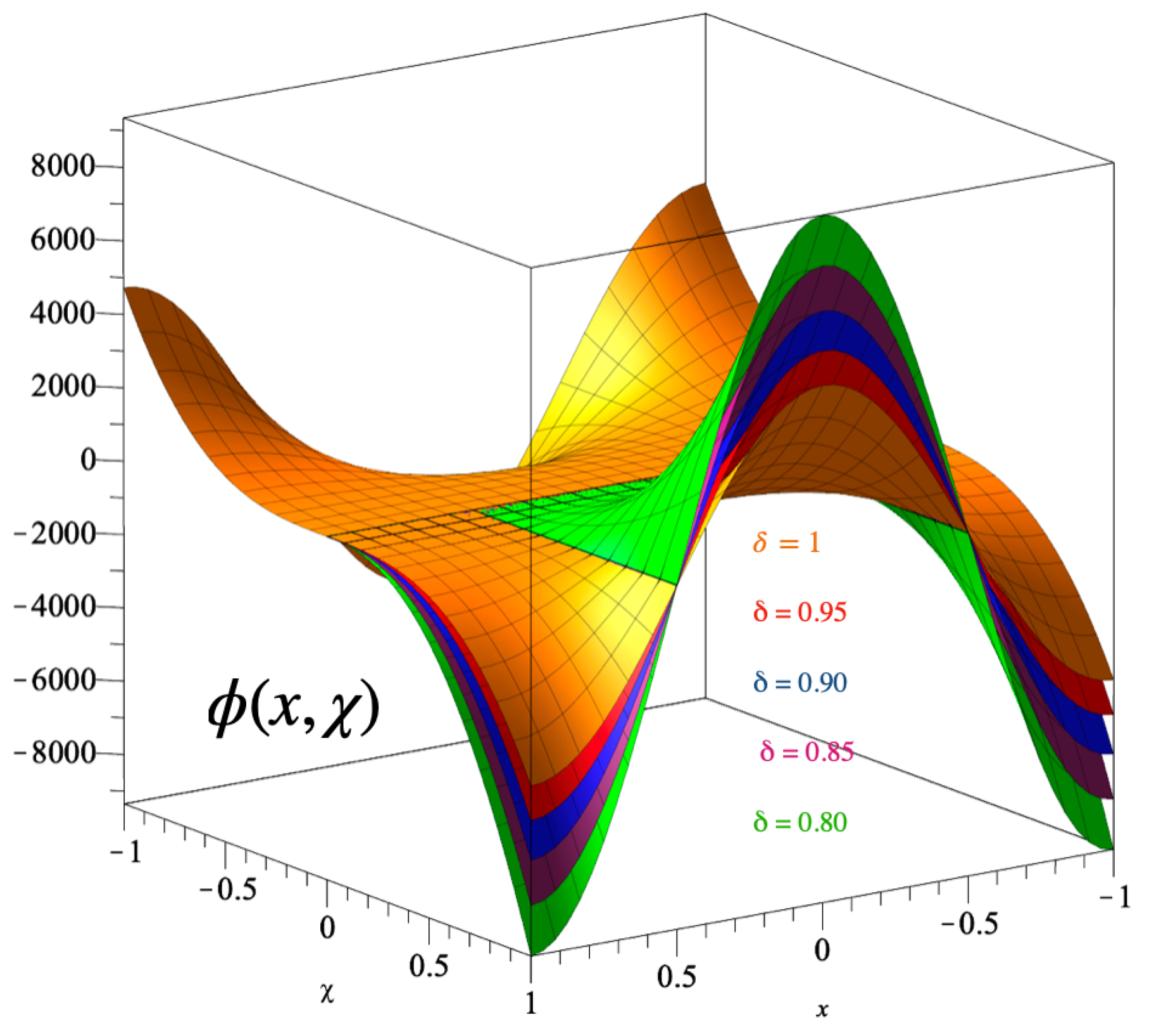
([26]). The fractional dKdV equation, accompanied by the prescribed initial condition is formulated the following way:

$${\displaystyle \frac{{\partial }^{\delta }\varphi }{\partial {\chi }^{\delta }}}+{\displaystyle \frac{{\partial }^3\varphi }{\partial x^3}}=-sin\left(\pi x\right)sin\left(\chi \right)-{\pi }^{3}cos\left(\pi x\right)cos\left(\chi \right),x,\chi >0,0<\delta \le 1$$

(30)

and

$$\varphi (x,0)=sin\left(\pi x\right).$$

(31)

On utilizing NGLT for Equation (30) and using NT for Equation (31), it follows that

$$\begin{array}{cc}\hfill {\displaystyle \frac{\mathsf{\Phi }(p;u,s)}{s^{\delta }}}& -s^{\alpha -\delta +1}\mathsf{\Phi }(p;u)\hfill \\ \hfill & =-N_x^{+}{G}_{\alpha }\left[{\displaystyle \frac{{\partial }^3\varphi }{\partial x^3}}\right]+N_x^{+}{G}_{\alpha }\left[sin\left(\pi x\right)sin\left(\chi \right)-{\pi }^{3}cos\left(\pi x\right)cos\left(\chi \right)\right].\hfill \end{array}$$

(32)

By multiplying both sides of Equation (32) by $s^{\delta }$ and substituting the Natural transform of the initial condition, we derive the following expression:

$$\begin{array}{ccc}\hfill \mathsf{\Phi }(p;u,s)& =& {\displaystyle \frac{\pi s^{\alpha +1}u}{p^2+u^2{\pi }^2}}-s^{\delta }{N}_x^{+}{G}_{\alpha }\left[{\displaystyle \frac{{\partial }^3\varphi }{\partial x^3}}\right]\hfill \\ & & +s^{\delta }{N}_x^{+}{G}_{\alpha }\left[sin\left(\pi x\right)sin\left(\chi \right)-{\pi }^{3}cos\left(\pi x\right)cos\left(\chi \right)\right].\hfill \end{array}$$

(33)

Using the series expansions for $sin\left(\chi \right)$ and $cos\left(\chi \right)$ in Equation (33), we obtain

$$\begin{array}{ccc}\hfill \mathsf{\Phi }(p;u,s)& =& {\displaystyle \frac{\pi s^{\alpha +1}u}{p^2+u^2{\pi }^2}}-s^{\delta }{N}_x^{+}{G}_{\alpha }\left[{\displaystyle \frac{{\partial }^3\varphi }{\partial x^3}}\right]\hfill \\ & & -s^{\delta }{N}_x^{+}{G}_{\alpha }\left[sin\left(\pi x\right)\left(\chi -{\displaystyle \frac{{\chi }^3}{3!}}+{\displaystyle \frac{{\chi }^5}{5!}}-{\displaystyle \frac{{\chi }^7}{7!}}+\dots \right)\right]\hfill \\ & & -s^{\delta }{N}_x^{+}{G}_{\alpha }\left[{\pi }^{3}cos\left(\pi x\right)\left(1-{\displaystyle \frac{{\chi }^2}{2!}}+{\displaystyle \frac{{\chi }^4}{4!}}-{\displaystyle \frac{{\chi }^6}{6!}}+\dots \right)\right],\hfill \end{array}$$

(34)

and so

$$\begin{array}{ccc}\hfill \mathsf{\Phi }(p;u,s)& =& {\displaystyle \frac{\pi s^{\alpha +1}u}{p^2+u^2{\pi }^2}}-s^{\delta }{N}_x^{+}{G}_{\alpha }\left[{\displaystyle \frac{{\partial }^3\varphi }{\partial x^3}}\right]\hfill \\ & & -{\displaystyle \frac{\pi s^{\alpha +1}u}{p^2+u^2{\pi }^2}}\left(s^{\delta +\alpha +2}-s^{\delta +\alpha +4}+s^{\delta +\alpha +6}-s^{\delta +\alpha +8}+\dots \right)\hfill \\ & & -\left[{\displaystyle \frac{{\pi }^{3}p}{p^2+u^2{\pi }^2}}\left(s^{\delta +\alpha +1}-s^{\delta +\alpha +3}+s^{\delta +\alpha +5}-s^{\delta +\alpha +7}+\dots \right)\right].\hfill \end{array}$$

(35)

By applying the INGLT to Equation (35) followed by the implementation of the Adomian Decomposition Method (ADM), we obtain

$$\begin{array}{ccc}\hfill \sum _{n=0}^{\infty }{\varphi }_n(x,\chi )& =& sin\left(\pi x\right)-sin\left(\pi x\right)\left({\displaystyle \frac{{\chi }^{\delta +1}}{\Gamma (\delta +2)}}-{\displaystyle \frac{{\chi }^{\delta +3}}{\Gamma (\delta +4)}}+{\displaystyle \frac{{\chi }^{\delta +5}}{\Gamma (\delta +6)}}-{\displaystyle \frac{{\chi }^{\delta +7}}{\Gamma (\delta +8)}}+\dots \right)\hfill \\ & & -{\pi }^{3}cos\left(\pi x\right)\left({\displaystyle \frac{{\chi }^{\delta }}{\Gamma (\delta +1)}}-{\displaystyle \frac{{\chi }^{\delta +2}}{\Gamma (\delta +3)}}+{\displaystyle \frac{{\chi }^{\delta +4}}{\Gamma (\delta +5)}}-{\displaystyle \frac{{\chi }^{\delta +6}}{\Gamma (\delta +7)}}+\dots \right)\hfill \\ & & -N_{p,u}^{-1}{G}_s^{-1}\left[N_x^{+}{G}_{\alpha }\left[\sum _{n=0}^{\infty }{\displaystyle \frac{{\partial }^3{\varphi }_n}{\partial x^3}}\right]\right].\hfill \end{array}$$

$$\begin{array}{ccc}\hfill {\varphi }_0(x,\chi )& =& sin\left(\pi x\right)-sin\left(\pi x\right)\left({\displaystyle \frac{{\chi }^{\delta +1}}{\Gamma (\delta +2)}}-{\displaystyle \frac{{\chi }^{\delta +3}}{\Gamma (\delta +4)}}+{\displaystyle \frac{{\chi }^{\delta +5}}{\Gamma (\delta +6)}}-{\displaystyle \frac{{\chi }^{\delta +7}}{\Gamma (\delta +8)}}+\dots \right)\hfill \\ & & -{\pi }^{3}cos\left(\pi x\right)\left({\displaystyle \frac{{\chi }^{\delta }}{\Gamma (\delta +1)}}-{\displaystyle \frac{{\chi }^{\delta +2}}{\Gamma (\delta +3)}}+{\displaystyle \frac{{\chi }^{\delta +4}}{\Gamma (\delta +5)}}-{\displaystyle \frac{{\chi }^{\delta +6}}{\Gamma (\delta +7)}}+\dots \right)\hfill \end{array}$$

and

$${\varphi }_{n+1}(x,\chi )=-N_{p,u}^{-1}{G}_s^{-1}\left[s^{\delta }{N}_x^{+}{G}_{\alpha }\left[\sum _{n=0}^{\infty }{\displaystyle \frac{{\partial }^3{\varphi }_n}{\partial x^3}}\right]\right].$$

(36)

where $n\ge 0,$ This is how the first two terms of the sequence are written:

$$\begin{array}{cc}\hfill & {\varphi }_1\left(x,\chi \right)\hfill \\ & =-N_{p,u}^{-1}{G}_s^{-1}\left[s^{\delta }{N}_x^{+}{G}_{\alpha }\left[\sum _{n=0}^{\infty }{\displaystyle \frac{{\partial }^3{\varphi }_0}{\partial x^3}}\right]\right]\hfill \\ \hfill & =N_{p,u}^{-1}{G}_s^{-1}\left[s^{\delta }{N}_x^{+}{G}_{\alpha }\left[{\pi }^{3}cos\left(\pi x\right)\right]\right]\hfill \\ & -N_{p,u}^{-1}{G}_s^{-1}\left[s^{\delta }{N}_x^{+}{G}_{\alpha }\left[{\pi }^{3}cos\left(\pi x\right)\left({\displaystyle \frac{{\chi }^{\delta +1}}{\Gamma \left(\delta +2\right)}}-{\displaystyle \frac{{\chi }^{\delta +3}}{\Gamma \left(\delta +4\right)}}+{\displaystyle \frac{{\chi }^{\delta +5}}{\Gamma \left(\delta +6\right)}}-{\displaystyle \frac{{\chi }^{\delta +7}}{\Gamma \left(\delta +8\right)}}+...\right)\right]\right]\hfill \\ \hfill & +N_{p,u}^{-1}{G}_s^{-1}\left[s^{\delta }{N}_x^{+}{G}_{\alpha }\left[{\pi }^{6}sin\left(\pi x\right)\left({\displaystyle \frac{{\chi }^{\delta }}{\Gamma \left(\delta +1\right)}}-{\displaystyle \frac{{\chi }^{\delta +2}}{\Gamma \left(\delta +3\right)}}+{\displaystyle \frac{{\chi }^{\delta +4}}{\Gamma \left(\delta +5\right)}}-{\displaystyle \frac{{\chi }^{\delta +6}}{\Gamma \left(\delta +7\right)}}+...\right)\right]\right]\hfill \end{array}$$

thus

$$\begin{array}{ccc}\hfill {\varphi }_1\left(x,\chi \right)& =& -N_{p,u}^{-1}{G}_s^{-1}\left[s^{\delta }{N}_x^{+}{G}_{\alpha }\left[\sum _{n=0}^{\infty }{\displaystyle \frac{{\partial }^3{\varphi }_0}{\partial x^3}}\right]\right]\hfill \\ & =& N_{p,u}^{-1}{G}_s^{-1}\left[{\displaystyle \frac{{\pi }^3{s}^{\alpha +\delta +1}p}{p^2+u^2{\pi }^2}}\right]\hfill \\ & & -N_{p,u}^{-1}{G}_s^{-1}\left[\left[{\displaystyle \frac{{\pi }^{3}p}{p^2+u^2{\pi }^2}}\left(\begin{array}{c}{s}^{\alpha +2\delta +2}-s^{\alpha +2\delta +4}\\ +s^{\alpha +2\delta +6}-s^{\alpha +2\delta +8}+...\end{array}\right)\right]\right]\hfill \\ & & +N_{p,u}^{-1}{G}_s^{-1}\left[s^{\delta }\left[{\displaystyle \frac{{\pi }^{6}u}{p^2+u^2{\pi }^2}}\left(\begin{array}{c}{s}^{\alpha +2\delta +1}-s^{\alpha +2\delta +3}\\ +s^{\alpha +2\delta +5}-s^{\alpha +2\delta +7}+...\end{array}\right)\right]\right].\hfill \end{array}$$

Hence,

$$\begin{array}{ccc}\hfill {\varphi }_1\left(x,\chi \right)& =& {\displaystyle \frac{{\pi }^3{\chi }^{\delta }}{\Gamma \left(\delta +1\right)}}cos\left(\pi x\right)-{\pi }^{3}cos\left(\pi x\right)\left[\left(\begin{array}{c}{\displaystyle \frac{{\chi }^{2\delta +1}}{\Gamma \left(2\delta +2\right)}}-{\displaystyle \frac{{\chi }^{2\delta +3}}{\Gamma \left(2\delta +4\right)}}\\ +{\displaystyle \frac{{\chi }^{2\delta +5}}{\Gamma \left(2\delta +6\right)}}-{\displaystyle \frac{{\chi }^{2\delta +7}}{\Gamma \left(2\delta +8\right)}}+...\end{array}\right)\right]\hfill \\ & & +{\pi }^{6}sin\left(\pi x\right)\left(\begin{array}{c}{\displaystyle \frac{{\chi }^{2\delta }}{\Gamma \left(2\delta +1\right)}}-{\displaystyle \frac{{\chi }^{2\delta +2}}{\Gamma \left(2\delta +3\right)}}\\ +{\displaystyle \frac{{\chi }^{2\delta +4}}{\Gamma \left(2\delta +5\right)}}-{\displaystyle \frac{{\chi }^{2\delta +6}}{\Gamma \left(2\delta +7\right)}}+...\end{array}\right)\hfill \end{array}$$

At $n=1,$ we have

$$\begin{array}{ccc}\hfill {\varphi }_2\left(x,\chi \right)& =& -N_{p,u}^{-1}{G}_s^{-1}\left[s^{\delta }{N}_x^{+}{G}_{\alpha }\left[{\displaystyle \frac{{\partial }^3{\varphi }_1}{\partial x^3}}\right]\right]\hfill \\ & =& -N_{p,u}^{-1}{G}_s^{-1}\left[s^{\delta }{N}_x^{+}{G}_{\alpha }\left[{\pi }^6{\displaystyle \frac{{\chi }^{\delta }}{\Gamma \left(\delta +1\right)}}sin\left(\pi x\right)\right]\right]\hfill \\ & & -N_{p,u}^{-1}{G}_s^{-1}\left[s^{\delta }{N}_x^{+}{G}_{\alpha }\left[{\pi }^{6}sin\left(\pi x\right)\left(\begin{array}{c}{\displaystyle \frac{{\chi }^{2\delta +1}}{\Gamma \left(2\delta +2\right)}}-{\displaystyle \frac{{\chi }^{2\delta +3}}{\Gamma \left(2\delta +4\right)}}\\ +{\displaystyle \frac{{\chi }^{2\delta +5}}{\Gamma \left(2\delta +6\right)}}-{\displaystyle \frac{{\chi }^{2\delta +7}}{\Gamma \left(2\delta +8\right)}}+...\end{array}\right)\right]\right]\hfill \\ & & -N_{p,u}^{-1}{G}_s^{-1}\left[s^{\delta }{N}_x^{+}{G}_{\alpha }\left[{\pi }^{9}cos\left(\pi x\right)\left(\begin{array}{c}{\displaystyle \frac{{\chi }^{2\delta }}{\Gamma \left(2\delta +1\right)}}-{\displaystyle \frac{{\chi }^{2\delta +2}}{\Gamma \left(2\delta +3\right)}}\\ +{\displaystyle \frac{{\chi }^{2\delta +4}}{\Gamma \left(2\delta +5\right)}}-{\displaystyle \frac{{\chi }^{2\delta +6}}{\Gamma \left(2\delta +7\right)}}+...\end{array}\right)\right]\right]\hfill \\ \hfill {\varphi }_2\left(x,\chi \right)& =& -{\displaystyle \frac{{\pi }^6{\chi }^{2\delta }}{\Gamma \left(2\delta +1\right)}}sin\left(\pi x\right)+{\pi }^{6}sin\left(\pi x\right)\left[\left(\begin{array}{c}{\displaystyle \frac{{\chi }^{3\delta +1}}{\Gamma \left(3\delta +2\right)}}-{\displaystyle \frac{{\chi }^{3\delta +3}}{\Gamma \left(3\delta +4\right)}}\\ +{\displaystyle \frac{{\chi }^{3\delta +5}}{\Gamma \left(3\delta +6\right)}}-{\displaystyle \frac{{\chi }^{3\delta +7}}{\Gamma \left(3\delta +8\right)}}+...\end{array}\right)\right]\hfill \\ & & +{\pi }^{9}cos\left(\pi x\right)\left({\displaystyle \frac{{\chi }^{3\delta }}{\Gamma \left(3\delta +1\right)}}-{\displaystyle \frac{{\chi }^{3\delta +2}}{\Gamma \left(3\delta +3\right)}}+{\displaystyle \frac{{\chi }^{3\delta +4}}{\Gamma \left(3\delta +5\right)}}-{\displaystyle \frac{{\chi }^{3\delta +6}}{\Gamma \left(3\delta +7\right)}}+...\right)\hfill \end{array}$$

Ultimately, the approximate solution to Equation (30) is represented by the following formulation:

$$\begin{array}{cc}\hfill \varphi \left(x,\chi \right)=& sin\left(\pi x\right)-sin\left(\pi x\right)\left({\displaystyle \frac{{\chi }^{\delta +1}}{\Gamma \left(\delta +2\right)}}-{\displaystyle \frac{{\chi }^{\delta +3}}{\Gamma \left(\delta +4\right)}}+{\displaystyle \frac{{\chi }^{\delta +5}}{\Gamma \left(\delta +6\right)}}-{\displaystyle \frac{{\chi }^{\delta +7}}{\Gamma \left(\delta +8\right)}}+...\right)\hfill \\ & -{\pi }^{3}cos\left(\pi x\right)\left({\displaystyle \frac{{\chi }^{\delta }}{\Gamma \left(\delta +1\right)}}-{\displaystyle \frac{{\chi }^{\delta +2}}{\Gamma \left(\delta +3\right)}}+{\displaystyle \frac{{\chi }^{\delta +4}}{\Gamma \left(\delta +5\right)}}-{\displaystyle \frac{{\chi }^{\delta +6}}{\Gamma \left(\delta +7\right)}}+...\right)\hfill \\ & +{\displaystyle \frac{{\pi }^3{\chi }^{\delta }}{\Gamma \left(\delta +1\right)}}cos\left(\pi x\right)\hfill \\ & -{\pi }^{3}cos\left(\pi x\right)\left[\left({\displaystyle \frac{{\chi }^{2\delta +1}}{\Gamma \left(2\delta +2\right)}}-{\displaystyle \frac{{\chi }^{2\delta +3}}{\Gamma \left(2\delta +4\right)}}+{\displaystyle \frac{{\chi }^{2\delta +5}}{\Gamma \left(2\delta +6\right)}}-{\displaystyle \frac{{\chi }^{2\delta +7}}{\Gamma \left(2\delta +8\right)}}+...\right)\right]\hfill \\ \hfill & +{\pi }^{6}sin\left(\pi x\right)\left({\displaystyle \frac{{\chi }^{2\delta }}{\Gamma \left(2\delta +1\right)}}-{\displaystyle \frac{{\chi }^{2\delta +2}}{\Gamma \left(2\delta +3\right)}}+{\displaystyle \frac{{\chi }^{2\delta +4}}{\Gamma \left(2\delta +5\right)}}-{\displaystyle \frac{{\chi }^{2\delta +6}}{\Gamma \left(2\delta +7\right)}}+...\right)\hfill \\ & -{\displaystyle \frac{{\pi }^6{\chi }^{2\delta }}{\Gamma \left(2\delta +1\right)}}sin\left(\pi x\right)\hfill \\ \hfill & +{\pi }^{6}sin\left(\pi x\right)\left[\left({\displaystyle \frac{{\chi }^{3\delta +1}}{\Gamma \left(3\delta +2\right)}}-{\displaystyle \frac{{\chi }^{3\delta +3}}{\Gamma \left(3\delta +4\right)}}+{\displaystyle \frac{{\chi }^{3\delta +5}}{\Gamma \left(3\delta +6\right)}}-{\displaystyle \frac{{\chi }^{3\delta +7}}{\Gamma \left(3\delta +8\right)}}+...\right)\right]\hfill \\ \hfill & +{\pi }^{9}cos\left(\pi x\right)\left({\displaystyle \frac{{\chi }^{3\delta }}{\Gamma \left(3\delta +1\right)}}-{\displaystyle \frac{{\chi }^{3\delta +2}}{\Gamma \left(3\delta +3\right)}}+{\displaystyle \frac{{\chi }^{3\delta +4}}{\Gamma \left(3\delta +5\right)}}-{\displaystyle \frac{{\chi }^{3\delta +6}}{\Gamma \left(3\delta +7\right)}}+...\right)\hfill \end{array}$$

Accordingly, the exact solution corresponding to $\delta =1$ is represented by the following expression:

$$\begin{array}{ccc}\hfill \varphi \left(x,\chi \right)& =& sin\left(\pi x\right)-sin\left(\pi x\right)\left({\displaystyle \frac{{\chi }^2}{\Gamma \left(3\right)}}-{\displaystyle \frac{{\chi }^4}{\Gamma \left(5\right)}}+{\displaystyle \frac{{\chi }^6}{\Gamma \left(7\right)}}-{\displaystyle \frac{{\chi }^8}{\Gamma \left(7\right)}}+...\right)\hfill \\ & =& sin\left(\pi x\right)\left(1-{\displaystyle \frac{{\chi }^2}{\Gamma \left(3\right)}}+{\displaystyle \frac{{\chi }^4}{\Gamma \left(5\right)}}-{\displaystyle \frac{{\chi }^6}{\Gamma \left(7\right)}}+{\displaystyle \frac{{\chi }^8}{\Gamma \left(7\right)}}-...\right)\hfill \end{array}$$

$$\varphi \left(x,\chi \right)=sin\left(\pi x\right)cos\left(\chi \right)$$

Figure 1 depicts the behavior of $\varphi (x,\chi )$ for $x,\chi \in [-1,1]$ at various values of δ, showing that the approximate solutions converge closely to the exact solution.

Next, we introduce the NGLTDM, which is used to study and solve the nonlinear fractional dKdV equation.

• Problem: Think about the nonlinear one-dimensional fractional dKdV equation, which is defined by the starting point:

  $${\displaystyle \frac{{\partial }^{\delta }\varphi }{\partial {\chi }^{\delta }}}+a{\displaystyle \frac{{\partial }^3\varphi }{\partial x^3}}+b\varphi {\displaystyle \frac{\partial \varphi }{\partial x}}=f(x,\chi ),$$

  (37)

  with

  $$\varphi (x,0)=f_1\left(x\right),$$

  (38)

  where $f(x,\chi )$ and $f_1\left(x\right)$ are given functions, and a and b are constants.
  To obtain the solution of Equation (37), we apply the NGLTDM, which yields

  $$\varphi (x,\chi )=N_{p,u}^{-1}{G}_s^{-1}\left[s^{\alpha +1}{F}_1(p;u)+s^{\delta }F(p;u,s)\right]-N_{p,u}^{-1}{G}_s^{-1}\left[s^{\delta }{N}_x^{+}{G}_{\alpha }\left(a{\displaystyle \frac{{\partial }^3\varphi }{\partial x^3}}+b\varphi {\displaystyle \frac{\partial \varphi }{\partial x}}\right)\right],$$

  (39)

  where $F_1(p;u)$ is the Natural Transform of $f_1\left(x\right)$, and $F(p;u,s)$ is the Natural Generalized-Laplace Transform of $f(x,\chi )$.
• Applying the decomposition approach gives

  $$\begin{array}{ccc}\hfill \sum _{n=0}^{\infty }{\varphi }_n(x,\chi )& =& N_{p,u}^{-1}{G}_s^{-1}\left[s^{\alpha +1}{F}_1(p;u)+s^{\delta }F(p;u,s)\right]\hfill \\ & & -N_{p,u}^{-1}{G}_s^{-1}\left[s^{\delta }{N}_x^{+}{G}_{\alpha }\left(a\sum _{n=0}^{\infty }{\displaystyle \frac{{\partial }^3{\varphi }_n}{\partial x^3}}+b\sum _{n=0}^{\infty }{\varphi }_n{\displaystyle \frac{\partial {\varphi }_n}{\partial x}}\right)\right].\hfill \end{array}$$

  (40)

  The initial term of the series is given by

  $${\varphi }_0=N_{p,u}^{-1}{G}_s^{-1}\left[s^{\alpha +1}{F}_1(p;u)+s^{\delta }F(p;u,s)\right],$$

  (41)

  and the recursive relation for subsequent terms is expressed as

  $${\varphi }_{n+1}=-N_{p,u}^{-1}{G}_s^{-1}\left[s^{\delta }{N}_x^{+}{G}_{\alpha }\left(a{\displaystyle \frac{{\partial }^3{\varphi }_n}{\partial x^3}}+b{A}_n\right)\right],$$

  (42)

  where $A_n={\sum }_{n=0}^{\infty }\left({\varphi }_n{\displaystyle \frac{\partial {\varphi }_n}{\partial x}}\right)$, and the first few Adomian polynomials are:

  $$\begin{array}{ccc}\hfill A_0& =& {\varphi }_0{\varphi }_{0x},\hfill \\ \hfill A_1& =& {\varphi }_{0x}{\varphi }_1+{\varphi }_0{\varphi }_{1x},\hfill \\ \hfill A_2& =& {\varphi }_{0x}{\varphi }_2+{\varphi }_0{\varphi }_{2x}+{\varphi }_1{\varphi }_{1x},\hfill \\ \hfill A_3& =& {\varphi }_{0x}{\varphi }_3+{\varphi }_0{\varphi }_{3x}+{\varphi }_{1x}{\varphi }_2+{\varphi }_1{\varphi }_{2x}.\hfill \end{array}$$

  (43)

  Hence, the approximate solution of Equation (37) can be expressed as

  $$\varphi (x,\chi )={\varphi }_0+{\varphi }_1+{\varphi }_2+\dots$$

  By setting $a=1$, $b=-2$, and $f(x,\chi )=0$ in Equation (37), We get the following example to help us understand.

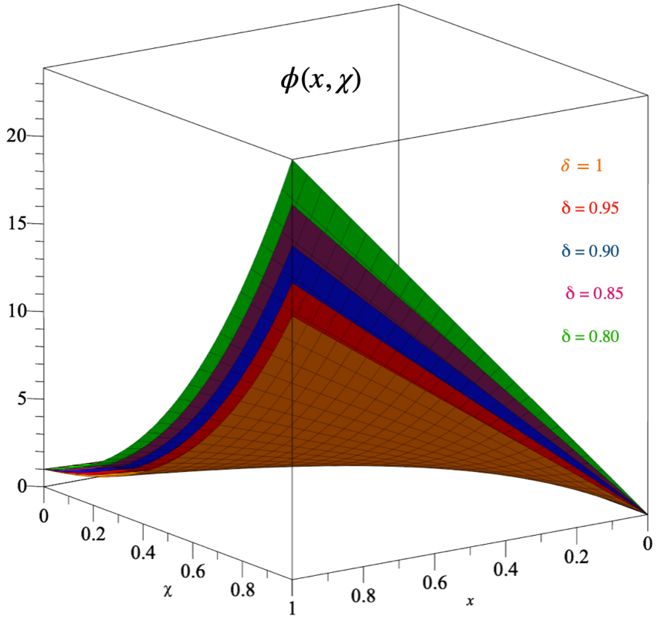
Example 3.

Take into account the following nonlinear one-dimensional fractional dKdV equation with the initial condition:

$${\displaystyle \frac{{\partial }^{\delta }\varphi }{\partial {\chi }^{\delta }}}+{\displaystyle \frac{{\partial }^3\varphi }{\partial x^3}}-2\varphi {\varphi }_x=0,$$

(44)

and

$$\varphi (x,0)=x.$$

(45)

By using Equations (41) and (42), we can obtain

$${\varphi }_0=x.$$

(46)

The remaining components are derived using

$${\varphi }_{n+1}(x,\chi )=-N_{p,u}^{-1}{G}_s^{-1}\left[s^{\delta }{N}_x^{+}{G}_{\alpha }\left({\displaystyle \frac{{\partial }^3{\varphi }_n}{\partial x^3}}\right)\right]+G_2^{-1}\left[s^{\delta }{G}_2\left(2A_n\right)\right],$$

(47)

By substituting $n=0$ into Equation (47), we obtain the following result:

$$\begin{array}{ccc}\hfill {\varphi }_1(x,\chi )& =& -N_{p,u}^{-1}{G}_s^{-1}\left[s^{\delta }{N}_x^{+}{G}_{\alpha }\left({\displaystyle \frac{{\partial }^3{\varphi }_0}{\partial x^3}}\right)\right]+N_{p,u}^{-1}{G}_s^{-1}\left[s^{\delta }{N}_x^{+}{G}_{\alpha }\left(2A_0\right)\right]\hfill \\ & =& -N_{p,u}^{-1}{G}_s^{-1}\left[s^{\delta }{N}_x^{+}{G}_{\alpha }\left(0\right)\right]+N_{p,u}^{-1}{G}_s^{-1}\left[s^{\delta }{N}_x^{+}{G}_{\alpha }\left(2{\varphi }_0{\varphi }_{0x}\right)\right]\hfill \\ & =& N_{p,u}^{-1}{G}_s^{-1}\left[s^{\delta }{N}_x^{+}{G}_{\alpha }\left(2x\right)\right]\hfill \\ & =& N_{p,u}^{-1}{G}_s^{-1}\left[{\displaystyle \frac{2u}{p^2}}{s}^{\delta +\alpha +1}\right],\hfill \\ \hfill {\varphi }_1(x,\chi )& =& 2x{\displaystyle \frac{{\chi }^{\delta }}{\Gamma (\delta +1)}}.\hfill \end{array}$$

At $n=1$:

$$\begin{array}{ccc}\hfill {\varphi }_2(x,\chi )& =& -N_{p,u}^{-1}{G}_s^{-1}\left[s^{\delta }{N}_x^{+}{G}_{\alpha }\left({\displaystyle \frac{{\partial }^3{\varphi }_1}{\partial x^3}}\right)\right]+N_{p,u}^{-1}{G}_s^{-1}\left[s^{\delta }{N}_x^{+}{G}_{\alpha }\left(2A_1\right)\right]\hfill \\ & =& 2N_{p,u}^{-1}{G}_s^{-1}\left[s^{\delta }{N}_x^{+}{G}_{\alpha }({\varphi }_0{\varphi }_{1x}+{\varphi }_1{\varphi }_{0x})\right]\hfill \\ & =& N_{p,u}^{-1}{G}_s^{-1}\left[s^{\delta }{N}_x^{+}{G}_{\alpha }\left(8x{\displaystyle \frac{{\chi }^{\delta }}{\Gamma (\delta +1)}}\right)\right]\hfill \\ & =& N_{p,u}^{-1}{G}_s^{-1}\left[{\displaystyle \frac{8u}{p^2}}{s}^{2\delta +\alpha +1}\right],\hfill \\ \hfill {\varphi }_2(x,\chi )& =& 8x{\displaystyle \frac{{\chi }^{2\delta }}{\Gamma (2\delta +1)}}.\hfill \end{array}$$

At $n=2$:

$$\begin{array}{ccc}\hfill {\varphi }_3(x,\chi )& =& -N_{p,u}^{-1}{G}_s^{-1}\left[s^{\delta }{N}_x^{+}{G}_{\alpha }\left({\displaystyle \frac{{\partial }^3{\varphi }_1}{\partial x^3}}\right)\right]+N_{p,u}^{-1}{G}_s^{-1}\left[s^{\delta }{N}_x^{+}{G}_{\alpha }\left(2A_2\right)\right]\hfill \\ & =& N_{p,u}^{-1}{G}_s^{-1}\left[s^{\delta }{N}_x^{+}{G}_{\alpha }\left(32x{\displaystyle \frac{{\chi }^{2\delta }}{\Gamma (2\delta +1)}}+8x{\displaystyle \frac{{\chi }^{2\delta }}{\Gamma (\delta +1)\Gamma (\delta +1)}}\right)\right]\hfill \\ & =& N_{p,u}^{-1}{G}_s^{-1}\left[{\displaystyle \frac{32u}{p^2}}{s}^{3\delta +\alpha +1}+{\displaystyle \frac{8u}{p^2}}{s}^{3\delta +\alpha +1}{\displaystyle \frac{\Gamma (2\delta +1)}{\Gamma (\delta +1)\Gamma (\delta +1)}}\right]\hfill \\ & =& 32x{\displaystyle \frac{{\chi }^{3\delta }}{\Gamma (3\delta +1)}}+8x{\displaystyle \frac{{\chi }^{3\delta }\Gamma (2\delta +1)}{\Gamma (\delta +1)\Gamma (\delta +1)\Gamma (3\delta +1)}}.\hfill \end{array}$$

Accordingly, the approximate solution to Equation (44) is given by:

$$\begin{array}{ccc}\hfill \varphi (x,\chi )& =& x+2x{\displaystyle \frac{{\chi }^{\delta }}{\Gamma (\delta +1)}}+8x{\displaystyle \frac{{\chi }^{2\delta }}{\Gamma (2\delta +1)}}\hfill \\ & & +32x{\displaystyle \frac{{\chi }^{3\delta }}{\Gamma (3\delta +1)}}+8x{\displaystyle \frac{{\chi }^{3\delta }\Gamma (2\delta +1)}{\Gamma (\delta +1)\Gamma (\delta +1)\Gamma (3\delta +1)}}+\dots \hfill \end{array}$$

In Figure 2, we give the plots of $\varphi (x,\chi )$ for different values of $\delta .$ In particular, when $\delta =1$, we obtain:

$$\begin{array}{ccc}\hfill \varphi (x,\chi )& =& x+2x\chi +4x{\chi }^2+8x{\chi }^3+\dots \hfill \\ & =& x\left(1+2\chi +{\left(2\chi \right)}^2+{\left(2\chi \right)}^3+\dots \right)\hfill \\ & =& {\displaystyle \frac{x}{1-2\chi }}.\hfill \end{array}$$

The result is consistent with the findings reported in [7]. Figure 2 illustrates the plots of $\varphi (x,\chi )$ for $x,\chi \in [0,1]$ at different values of δ, showing the influence of the fractional parameter on the solution behavior. It demonstrates that as δ varies, the approximate solutions converge smoothly and consistently toward the exact solution.

5. Application of DNGLTDM to Fractional Two-Dimensional Dispersive KdV Equation

This section employs the DNGLTDM to solve third-order two-dimensional fractional dispersive partial differential equations.

Let us examine the following two-dimensional dKdV equation with a linear form and an initial condition:

$$D_{\chi }^{\delta }\varphi +L\varphi (x,y,\chi )=f(x,y,\chi ),x,y,\chi >0,0<\delta \le 1,$$

(48)

and

$$\varphi (x,y,0)=f_1(x,y).$$

(49)

Here, $D_{\chi }^{\delta }$ denotes the Caputo fractional operator, L represents the linear differential operator, and $f(x,y,\chi )$ corresponds to the external source term.

To investigate the solution of Equation (48), the following analytical steps are systematically outlined to guide the application of DNGLTDM and ensure a rigorous procedure for solving the associated fractional dispersive partial differential equation.

• Step 1: Applying the Double Natural Generalized-Laplace Transform (DNGLT) to Equation (48) gives

  $$N_2^{+}{G}_{\alpha }\left[D_{\chi }^{\delta }\varphi \right]+N_2^{+}{G}_{\alpha }\left[L\varphi (x,y,\chi )\right]=N_2^{+}{G}_{\alpha }\left[f(x,y,\chi )\right].$$

  (50)
• Step 2: Using Equation (6), we obtain

  $${\displaystyle \frac{\mathsf{\Phi }(p;u,q;v,s)}{s^{\delta }}}-s^{\alpha -\delta +1}{N}_2^{+}\left[\varphi (x,y,0)\right]=-N_2^{+}{G}_{\alpha }\left[L\varphi (x,y,\chi )\right]+F(p;u,q;v,s),$$

  (51)

  where $N_2^{+}\left[\varphi (x,y,0)\right]=F_1(p;u,q;v)$ and $N_2^{+}{G}_{\alpha }\left[f(x,y,\chi )\right]=F(p;u,q;v,s)$ are the DNT and the DNGLT of $f_1(x,y)$ and $f(x,y,\chi )$, respectively.
• Step 3: Multiplying Equation (51) by $s^{\delta }$, we obtain

  $$\mathsf{\Phi }(p;u,q;v,s)=s^{\alpha +1}{F}_1(p;u,q;v)-s^{\delta }{N}_2^{+}{G}_{\alpha }\left[L\varphi (x,y,\chi )\right]+s^{\delta }F(p;u,q;v,s).$$

  (52)
• Step 4: Applying the inverse DNGLT to Equation (52) yields

  $$\varphi (x,y,\chi )=g(x,y,\chi )-N_2^{-1}{G}_s^{-1}\left[s^{\delta }{N}_{x,y}^{+}{G}_{\alpha }\left[L\varphi (x,y,\chi )\right]\right],$$

  (53)

  where $N_2^{-1}{G}_s^{-1}=N_{p,u,q;v}^{-1}{G}_s^{-1}$.
• Step 5: The function $g(x,y,\chi )$ represents the contribution from the source term and initial condition. For the linear component, the following decomposition series solution is proposed:

  $$\varphi (x,y,\chi )=\sum _{n=0}^{\infty }{\varphi }_n(x,y,\chi ).$$

  (54)

  Substituting Equation (54) into Equation (53) gives

  $$\sum _{n=0}^{\infty }{\varphi }_n(x,y,\chi )=g(x,y,\chi )-N_2^{-1}{G}_s^{-1}\left[s^{\delta }{N}_{x,y}^{+}{G}_{\alpha }\left[L\sum _{n=0}^{\infty }{\varphi }_n(x,y,\chi )\right]\right].$$

  (55)

  Therefore, the required recursive relations are:

  $${\varphi }_0(x,y,\chi )=g(x,y,\chi ),$$

  (56)

  and

  $${\varphi }_{n+1}(x,y,\chi )=-N_2^{-1}{G}_s^{-1}\left[s^{\delta }{N}_{x,y}^{+}{G}_{\alpha }\left[L{\varphi }_n(x,y,\chi )\right]\right].$$

  (57)

We presume the existence of IDNGLT for each term in the aforementioned equations. In the next example, the DNGLTDM is used to solve dkdv in three-dimensional space, especially when the initial conditions are given.

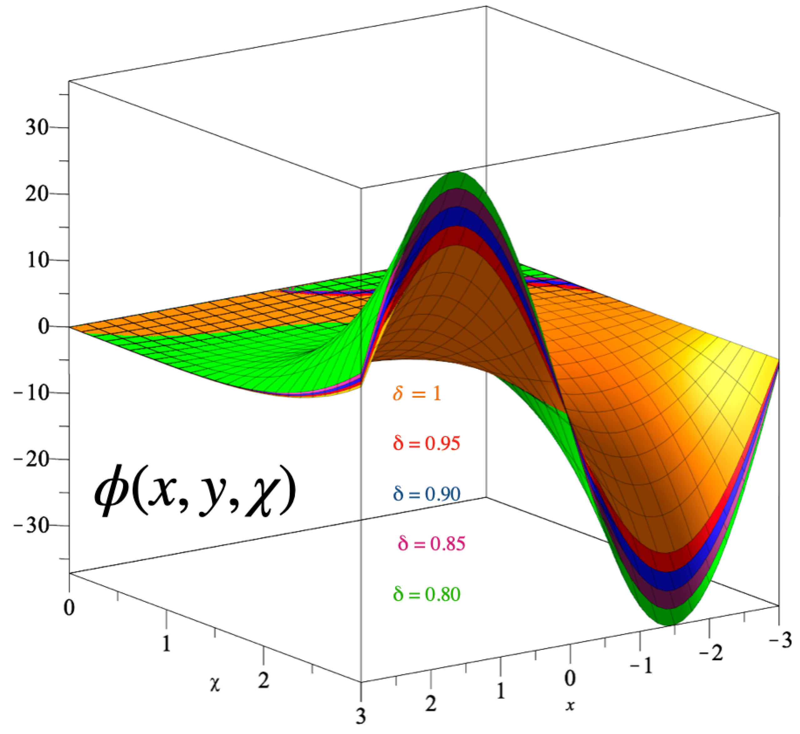
Example 4.

Consider the non-homogeneous fractional dkdv in two-dimensional space with the initial condition:

$$\begin{array}{ccc}\hfill {\displaystyle \frac{{\partial }^{\delta }\varphi }{\partial {\chi }^{\delta }}}+{\displaystyle \frac{{\partial }^3\varphi }{\partial x^3}}+{\displaystyle \frac{{\partial }^3\varphi }{\partial y^3}}& =& sin(x+y)cos\left(\chi \right)-2cos(x+y)sin\left(\chi \right),\hfill \end{array}$$

(58)

and

$$\varphi (x,y,0)=0.$$

(59)

By employing the previously described DNGLTDM to Equation (58), we obtain the following series representation for the solution:

$$\begin{array}{ccc}\hfill \sum _{n=0}^{\infty }{\varphi }_n& =& N_2^{-1}{G}_s^{-1}\left[{\displaystyle \frac{(pv+qu)}{(p^2+u^2)(q^2+v^2)}}\left(s^{\alpha +\delta +2}-s^{\alpha +\delta +4}+s^{\alpha +\delta +6}-s^{\alpha +\delta +8}+\dots \right)\right]\hfill \\ & & -2N_2^{-1}{G}_s^{-1}\left[{\displaystyle \frac{(pq-uv)}{(p^2+u^2)(q^2+v^2)}}\left(s^{\alpha +\delta +1}-s^{\alpha +\delta +3}+s^{\alpha +\delta +5}-s^{\alpha +\delta +7}+\dots \right)\right]\hfill \\ & & -N_2^{-1}{G}_s^{-1}\left[s^{\delta }{N}_2^{+}{G}_{\alpha }\left(\sum _{n=0}^{\infty }{\displaystyle \frac{{\partial }^3{\varphi }_n}{\partial x^3}}+\sum _{n=0}^{\infty }{\displaystyle \frac{{\partial }^3{\varphi }_n}{\partial y^3}}\right)\right].\hfill \end{array}$$

(60)

We get the following by running the inverse on the right side:

$$\begin{array}{ccc}\hfill \sum _{n=0}^{\infty }{\varphi }_n& =& sin(x+y)\left({\displaystyle \frac{{\chi }^{\delta +1}}{\Gamma (\delta +2)}}-{\displaystyle \frac{{\chi }^{\delta +3}}{\Gamma (\delta +4)}}+{\displaystyle \frac{{\chi }^{\delta +5}}{\Gamma (\delta +6)}}-{\displaystyle \frac{{\chi }^{\delta +7}}{\Gamma (\delta +8)}}+\dots \right)\hfill \\ & & -2cos(x+y)\left({\displaystyle \frac{{\chi }^{\delta }}{\Gamma (\delta +1)}}-{\displaystyle \frac{{\chi }^{\delta +2}}{\Gamma (\delta +3)}}+{\displaystyle \frac{{\chi }^{\delta +4}}{\Gamma (\delta +5)}}-{\displaystyle \frac{{\chi }^{\delta +6}}{\Gamma (\delta +7)}}+\dots \right)\hfill \\ & & -N_2^{-1}{G}_s^{-1}\left[s^{\delta }{N}_2^{+}{G}_{\alpha }\left(\sum _{n=0}^{\infty }{\displaystyle \frac{{\partial }^3{\varphi }_n}{\partial x^3}}+\sum _{n=0}^{\infty }{\displaystyle \frac{{\partial }^3{\varphi }_n}{\partial y^3}}\right)\right].\hfill \end{array}$$

(61)

The first component is given by

$$\begin{array}{ccc}\hfill {\varphi }_0& =& sin(x+y)\left({\displaystyle \frac{{\chi }^{\delta }}{\Gamma (\delta +1)}}-{\displaystyle \frac{{\chi }^{\delta +2}}{\Gamma (\delta +3)}}+{\displaystyle \frac{{\chi }^{\delta +4}}{\Gamma (\delta +5)}}-{\displaystyle \frac{{\chi }^{\delta +6}}{\Gamma (\delta +7)}}+\dots \right)\hfill \\ & & -2cos(x+y)\left({\displaystyle \frac{{\chi }^{\delta +1}}{\Gamma (\delta +2)}}-{\displaystyle \frac{{\chi }^{\delta +3}}{\Gamma (\delta +4)}}+{\displaystyle \frac{{\chi }^{\delta +5}}{\Gamma (\delta +6)}}-{\displaystyle \frac{{\chi }^{\delta +7}}{\Gamma (\delta +8)}}+\dots \right).\hfill \end{array}$$

(62)

The recursive elements are defined by

$${\varphi }_{n+1}=-N_2^{-1}{G}_s^{-1}\left[s^{\delta }{N}_2^{+}{G}_{\alpha }\left({\displaystyle \frac{{\partial }^3{\varphi }_n}{\partial x^3}}+{\displaystyle \frac{{\partial }^3{\varphi }_n}{\partial y^3}}\right)\right],n=0,1,2,\dots$$

(63)

At $n=0$, Equation (63) becomes

$${\varphi }_1=-N_2^{-1}{G}_s^{-1}\left[s^{\delta }{N}_2^{+}{G}_{\alpha }\left({\displaystyle \frac{{\partial }^3{\varphi }_0}{\partial x^3}}+{\displaystyle \frac{{\partial }^3{\varphi }_0}{\partial y^3}}\right)\right].$$

(64)

Hence, after simplification, we obtain:

$$\begin{array}{ccc}\hfill {\varphi }_1& =& 2cos(x+y)\left({\displaystyle \frac{{\chi }^{2\delta }}{\Gamma (2\delta +1)}}-{\displaystyle \frac{{\chi }^{2\delta +2}}{\Gamma (2\delta +3)}}+{\displaystyle \frac{{\chi }^{2\delta +4}}{\Gamma (2\delta +5)}}-{\displaystyle \frac{{\chi }^{2\delta +6}}{\Gamma (2\delta +7)}}+\dots \right)\hfill \\ & & +4sin(x+y)\left({\displaystyle \frac{{\chi }^{2\delta +1}}{\Gamma (2\delta +2)}}-{\displaystyle \frac{{\chi }^{2\delta +3}}{\Gamma (2\delta +4)}}+{\displaystyle \frac{{\chi }^{2\delta +5}}{\Gamma (2\delta +6)}}-{\displaystyle \frac{{\chi }^{2\delta +7}}{\Gamma (2\delta +8)}}+\dots \right).\hfill \end{array}$$

By substituting $n=1$ in Equation (63), we get

$$\begin{array}{ccc}\hfill {\varphi }_2& =& -4sin(x+y)\left({\displaystyle \frac{{\chi }^{3\delta }}{\Gamma (3\delta +1)}}-{\displaystyle \frac{{\chi }^{3\delta +2}}{\Gamma (3\delta +3)}}+{\displaystyle \frac{{\chi }^{3\delta +4}}{\Gamma (3\delta +5)}}-{\displaystyle \frac{{\chi }^{3\delta +6}}{\Gamma (3\delta +7)}}+\dots \right)\hfill \\ & & +8cos(x+y)\left({\displaystyle \frac{{\chi }^{3\delta +1}}{\Gamma (3\delta +2)}}-{\displaystyle \frac{{\chi }^{3\delta +3}}{\Gamma (3\delta +4)}}+{\displaystyle \frac{{\chi }^{3\delta +5}}{\Gamma (3\delta +6)}}-{\displaystyle \frac{{\chi }^{3\delta +7}}{\Gamma (3\delta +8)}}+\dots \right).\hfill \end{array}$$

Similarly, at $n=2$:

$$\begin{array}{ccc}\hfill {\varphi }_3& =& -8cos(x+y)\left({\displaystyle \frac{{\chi }^{4\delta }}{\Gamma (4\delta +1)}}-{\displaystyle \frac{{\chi }^{4\delta +2}}{\Gamma (4\delta +3)}}+{\displaystyle \frac{{\chi }^{4\delta +4}}{\Gamma (4\delta +5)}}-{\displaystyle \frac{{\chi }^{4\delta +6}}{\Gamma (4\delta +7)}}+\dots \right)\hfill \\ & & -16sin(x+y)\left({\displaystyle \frac{{\chi }^{4\delta +1}}{\Gamma (4\delta +2)}}-{\displaystyle \frac{{\chi }^{4\delta +3}}{\Gamma (4\delta +4)}}+{\displaystyle \frac{{\chi }^{4\delta +5}}{\Gamma (4\delta +6)}}-{\displaystyle \frac{{\chi }^{4\delta +7}}{\Gamma (4\delta +8)}}+\dots \right).\hfill \end{array}$$

From this, we derive the approximate solution:

$$\begin{array}{ccc}\hfill \varphi (x,y,\chi )& =& sin(x+y)\left({\displaystyle \frac{{\chi }^{\delta }}{\Gamma (\delta +1)}}-{\displaystyle \frac{{\chi }^{\delta +2}}{\Gamma (\delta +3)}}+{\displaystyle \frac{{\chi }^{\delta +4}}{\Gamma (\delta +5)}}-{\displaystyle \frac{{\chi }^{\delta +6}}{\Gamma (\delta +7)}}+\dots \right)\hfill \\ & & -2cos(x+y)\left({\displaystyle \frac{{\chi }^{\delta +1}}{\Gamma (\delta +2)}}-{\displaystyle \frac{{\chi }^{\delta +3}}{\Gamma (\delta +4)}}+{\displaystyle \frac{{\chi }^{\delta +5}}{\Gamma (\delta +6)}}-{\displaystyle \frac{{\chi }^{\delta +7}}{\Gamma (\delta +8)}}+\dots \right)\hfill \\ & & +2cos(x+y)\left({\displaystyle \frac{{\chi }^{2\delta }}{\Gamma (2\delta +1)}}-{\displaystyle \frac{{\chi }^{2\delta +2}}{\Gamma (2\delta +3)}}+{\displaystyle \frac{{\chi }^{2\delta +4}}{\Gamma (2\delta +5)}}-{\displaystyle \frac{{\chi }^{2\delta +6}}{\Gamma (2\delta +7)}}+\dots \right)\hfill \\ & & +4sin(x+y)\left({\displaystyle \frac{{\chi }^{2\delta +1}}{\Gamma (2\delta +2)}}-{\displaystyle \frac{{\chi }^{2\delta +3}}{\Gamma (2\delta +4)}}+{\displaystyle \frac{{\chi }^{2\delta +5}}{\Gamma (2\delta +6)}}-{\displaystyle \frac{{\chi }^{2\delta +7}}{\Gamma (2\delta +8)}}+\dots \right)\hfill \\ & & -4sin(x+y)\left({\displaystyle \frac{{\chi }^{3\delta }}{\Gamma (3\delta +1)}}-{\displaystyle \frac{{\chi }^{3\delta +2}}{\Gamma (3\delta +3)}}+{\displaystyle \frac{{\chi }^{3\delta +4}}{\Gamma (3\delta +5)}}-{\displaystyle \frac{{\chi }^{3\delta +6}}{\Gamma (3\delta +7)}}+\dots \right)\hfill \\ & & +8cos(x+y)\left({\displaystyle \frac{{\chi }^{3\delta +1}}{\Gamma (3\delta +2)}}-{\displaystyle \frac{{\chi }^{3\delta +3}}{\Gamma (3\delta +4)}}+{\displaystyle \frac{{\chi }^{3\delta +5}}{\Gamma (3\delta +6)}}-{\displaystyle \frac{{\chi }^{3\delta +7}}{\Gamma (3\delta +8)}}+\dots \right)\hfill \\ & & -8cos(x+y)\left({\displaystyle \frac{{\chi }^{4\delta }}{\Gamma (4\delta +1)}}-{\displaystyle \frac{{\chi }^{4\delta +2}}{\Gamma (4\delta +3)}}+{\displaystyle \frac{{\chi }^{4\delta +4}}{\Gamma (4\delta +5)}}-{\displaystyle \frac{{\chi }^{4\delta +6}}{\Gamma (4\delta +7)}}+\dots \right)\hfill \\ & & -16sin(x+y)\left({\displaystyle \frac{{\chi }^{4\delta +1}}{\Gamma (4\delta +2)}}-{\displaystyle \frac{{\chi }^{4\delta +3}}{\Gamma (4\delta +4)}}+{\displaystyle \frac{{\chi }^{4\delta +5}}{\Gamma (4\delta +6)}}-{\displaystyle \frac{{\chi }^{4\delta +7}}{\Gamma (4\delta +8)}}+\dots \right).\hfill \end{array}$$

$$\begin{array}{ccc}\hfill \varphi (x,y,\chi )& =& sin(x+y)\left({\displaystyle \frac{\chi }{\Gamma \left(2\right)}}-{\displaystyle \frac{{\chi }^3}{\Gamma \left(4\right)}}+{\displaystyle \frac{{\chi }^5}{\Gamma \left(6\right)}}-{\displaystyle \frac{{\chi }^7}{\Gamma \left(8\right)}}+\dots \right)\hfill \\ & =& sin(x+y)sin\left(\chi \right).\hfill \end{array}$$

Figure 3 presents the behavior of $\varphi (x,y,\chi )$ for $y=3$, $x\in [-3,3]$, and $\chi \in [0,3]$ at several values of δ. It clearly illustrates how variations in the fractional parameter δ affect the solution structure, showing that the approximate solutions converge smoothly toward the exact solution as δ increases.

6. Conclusions

This research presents a robust analytical methodology, the NGLTDM, which amalgamates the Natural Generalized-Laplace Transform with the Decomposition Method. The suggested method has been successfully used to solve fractional third-order dispersive partial differential equations. It provides an efficient and systematic way to find both exact and approximate solutions.

A number of examples are used to show that the method is accurate and works well with complex fractional systems. The resulting series solutions converge quickly and are very stable. Additionally, the developed method can be successfully generalized to a broader category of nonlinear fractional partial differential equations, with significant applications in multiple domains of applied mathematics, physics, and engineering.

References

- Shah, R.; Khan, H.; Arif, M.; Kumam, P. Application of Laplace–Adomian decomposition method for the analytical solution of third-order dispersive fractional partial differential equations. Entropy 2019, 21, 335. [Google Scholar] [CrossRef]
- Khan, A.; Akram, T.; Khan, A.; Ahmad, S.; Nonlaopon, K. Investigation of time fractional nonlinear KdV-Burgers equation under fractional operators with nonsingular kernels. AIMS Math 2023, 8, 1251–1268. [Google Scholar] [CrossRef]
- Kanth, A.; Aruna, K. Solution of fractional third-order dispersive partial differential equations. Egypt. J. Basic Appl. Sci. 2015, 2, 190–199. [Google Scholar] [CrossRef]
- Pandey, R.; Mishra, H. Homotopy analysis Sumudu transform method for time—Fractional third order dispersive partial differential equation. Adv. Comput. Math. 2017, 43, 365–383. [Google Scholar] [CrossRef]
- Bekela, A.; Deresse, A. An Efficient Numerical Method for Nonlinear Time Fractional Hyperbolic Partial Differential Equations Based on Fractional Shehu Transform Iterative Method. J. Appl. Math. 2025, 2025, 7007124. [Google Scholar] [CrossRef]
- Tandel, P.; Patel, A.; Patel, T. A Novel Computational Framework for Time-Fractional Higher-Order KdV Models: CLADM-Based Solutions and Comparative Analysis. Axioms 2025, 14, 511. [Google Scholar] [CrossRef]
- Eltayeb, H.; Alhefthi, R. Solution of Fractional Third-Order Dispersive Partial Differential Equations and Symmetric KdV via Sumudu–Generalized Laplace Transform Decomposition. Symmetry 2023, 15, 1540. [Google Scholar] [CrossRef]
- Appanah, R.; Abey Sherif, K. On Semi-Analytical Solutions for Linearized Dispersive KdV Equations. Mathematics 2020, 8, 1769. [Google Scholar] [CrossRef]
- Djidjeli, K.; Price, W.G.; Twizell, E.H.; Wang, Y. Numerical methods for the solution of the third-and fifth-order dispersive Korteweg-de Vries equations. Oceanogr. Lit. Rev. 1996, 2, 96. [Google Scholar] [CrossRef]
- Prakash, A.; Kumar, M. Numerical method for fractional dispersive partial differential equations. Commun. Numer. Anal 2017, 1, 1–18. [Google Scholar] [CrossRef]
- Sultana, T.; Khan, A.; Khandelwal, P. A new non-polynomial spline method for solution of linear and non-linear third order dispersive equations. Adv. Differ. Equations 2018, 2018, 316. [Google Scholar] [CrossRef]
- Abd-Elhameed, W.; Youssri, Y. Spectral tau solution of the linearized time-fractional KdV-Type equations. AIMS Math 2022, 7, 15138–15158. [Google Scholar] [CrossRef]
- Sahar, A.; Sumaira, Y.; Attra, A. Approximate Computation of Third-Order Dispersive Partial Differential Equation with Caputo Fractional Derivative. J. Xi’an Shiyou Univ. Nat. Sci. Ed. 2023, 19, 608–617. [Google Scholar]
- Rasheed, S.; Modanli, M.; Abdulazeez, S. Stability analysis and numerical implementation of the third-order fractional partial differential equation based on the caputo fractional derivative. J. Appl. Math. Comput. Mech. 2023, 22, 33–42. [Google Scholar] [CrossRef]
- Eltayeb, H. Application of Natural Generalized-Laplace Transform and Its Properties. Mathematics 2025, 13, 3194. [Google Scholar] [CrossRef]
- Obeidat, N.; Rawashdeh, M.; Al Erjani, M. A novel Adomian natural decomposition method with convergence analysis of nonlinear time-fractional differential equations. Int. J. Model. Simul. 2024, 1–16. [Google Scholar] [CrossRef]
- Sattaso, S.; Nonlaopon, K.; Kim, H. Further properties of Laplace-typed integral transforms. Dyn. Syst. Appl. 2019, 28, 195–215. [Google Scholar]
- Katatbeh, Q.; Belgacem, F. Applications of the Sumudu transform to fractional differential equations. Nonlinear Stud. 2011, 18, 99–112. [Google Scholar]
- Ghandehari, M.; Ranjbar, M. A numerical method for solving a fractional partial differential equation through converting it into an NLP problem. Comput. Math. Appl. 2013, 65, 975–982. [Google Scholar] [CrossRef]
- Bayrak, M.; Demir, A. A new approach for space-time fractional partial differential equations by residual power series method. Appl. Math. Comput. 2018, 336, 215–230. [Google Scholar] [CrossRef]
- Thabet, H.; Kendre, S. Analytical solutions for conformable space-time fractional partial differential equations via fractional differential transform. Chaos Solitons Fractals 2018, 109, 238–245. [Google Scholar] [CrossRef]
- Eltayeb, H.; Bachar, I.; Abdalla, Y. A note on time-fractional Navier–Stokes equation and multi-Laplace transform decomposition method. Adv. Differ. Equ. 2020, 2020, 519. [Google Scholar] [CrossRef]
- Eltayeb, H.; Aldossari, S. Solution of Time-Fractional Partial Differential Equations via the Natural Generalized Laplace Transform Decomposition Method. Fractal Fract. 2025, 9, 554. [Google Scholar] [CrossRef]
- Park, S. Revisit to Suzuki’s Metric Completenes. Nonlinear Convex Anal. Optim. Int. J. Numer. Comput. Appl. 2024, 3, 47–62. [Google Scholar]
- Jachymski, J.; Jozwik, I.; Terepeta, M. The Banach fixed point theorem: Selected topics from its hundred-year history. Rev. Real Acad. Cienc. Exactas Físicas Y Nat. Ser. A. Matemáticas 2024, 118, 140. [Google Scholar] [CrossRef]
- Kexue, L.; Jigen, P. Laplace transform and fractional differential equations. Appl. Math. Lett. 2011, 24, 2019–2023. [Google Scholar] [CrossRef]