Fractal-Guided Token Pruning for Efficient Vision Transformers

Abstract

Vision Transformers achieve strong performance across computer vision tasks but suffer from quadratic computational complexity with respect to token count, limiting deployment in resource-constrained environments. Existing token pruning methods rely on attention scores to identify important tokens, but attention mechanisms capture query-specific relevance rather than intrinsic information content, potentially discarding tokens that carry information for subsequent layers or different downstream tasks. We propose fractal-guided token pruning, a method that leverages the correlation dimension $D_{\mathrm{corr}}$ of token embeddings as a task-agnostic measure of geometric complexity. Our key insight is that tokens with high $D_{\mathrm{corr}}$ span higher-dimensional manifolds in representation space, indicating complex patterns, while tokens with low $D_{\mathrm{corr}}$ collapse to simpler structures representing redundant information. By computing a local $D_{\mathrm{corr}}$ for each token and pruning those with the lowest values, our method retains geometrically complex tokens independent of attention-based relevance. The correlation dimension quantifies how token embeddings fill the representation space: embeddings from uniform background regions cluster tightly in low-dimensional subspaces (low $D_{\mathrm{corr}}$), while embeddings from complex textures or object boundaries spread across higher-dimensional manifolds (high $D_{\mathrm{corr}}$), reflecting their richer information content. Experiments on CIFAR-10 and CIFAR-100 with fine-tuned ViT-B/16 models show that fractal-guided pruning consistently outperforms random and norm-based pruning across all tested ratios. At forty percent pruning, fractal pruning maintains 92.26% accuracy on CIFAR-10 with only a 0.99 percentage point drop from the 93.25% baseline while achieving 1.17× speedup. Our approach provides a geometry-based criterion for token importance that complements attention-based methods and shows promising generalization between CIFAR-10 and CIFAR-100 datasets.

1. Introduction

Vision Transformers [1] have emerged as a powerful architecture for computer vision tasks, achieving competitive or superior performance compared to convolutional neural networks [2,3] across image classification, object detection [4], and semantic segmentation [5]. The self-attention mechanism [6] at the core of Vision Transformers enables modeling of long-range dependencies between image patches, allowing the network to capture global context that is difficult for local convolution operations to access. However, this capability comes at a significant computational cost. The self-attention operation exhibits quadratic complexity with respect to the number of input tokens, making Vision Transformers computationally expensive for high-resolution images or resource-constrained deployment scenarios [7]. For a standard ViT-B/16 model processing a $224\times 224$ image, the input is divided into $14\times 14=196$ patch tokens, and computing attention across all token pairs requires ${196}^2=38,416$ pairwise interactions per attention head. This quadratic scaling limits the practical applicability of Vision Transformers in mobile devices, edge computing platforms, and real-time applications where computational resources and latency constraints are critical.

Token pruning has emerged as a promising approach to reduce the computational burden of Vision Transformers by dynamically removing redundant or less informative tokens during inference [8,9]. The key insight is that not all image patches contribute equally to the final prediction, and selectively retaining only the most important tokens can achieve substantial speedups with minimal accuracy degradation [10,11]. Existing token pruning methods primarily rely on attention mechanisms to assess token importance. For example, methods compute importance scores based on the attention weights from the class token to each patch token [8], under the assumption that tokens receiving higher attention are more relevant for classification. While these attention-based approaches have demonstrated effectiveness in reducing computational cost, they fundamentally measure query-specific relevance rather than intrinsic information content. A token may carry rich visual information about complex textures, object boundaries, or fine-grained details, but if it does not strongly attend to the current class token query, attention-based methods may incorrectly discard it. This limitation becomes particularly problematic in transfer learning scenarios where a pretrained model [12] is deployed across diverse downstream tasks with different query patterns, or in multi-task settings where different queries may require different subsets of tokens.

The central challenge in token pruning is to identify a measure of token importance that captures intrinsic information content independent of task-specific attention patterns. An ideal importance measure should reflect the geometric complexity and diversity of information encoded in each token’s representation [13,14], remaining stable across different downstream applications and query contexts. Such a measure would enable more robust token selection that preserves information-rich tokens beneficial for multiple tasks, rather than optimizing for a single query pattern. However, defining and computing such an intrinsic importance measure is non-trivial. Simple heuristics such as embedding norm or local variance may capture some aspects of information content, but they fail to account for the full geometric structure of how embeddings are distributed in the high-dimensional representation space [15]. A more principled approach requires analyzing the intrinsic dimensionality and complexity of the embedding distribution, which relates to fundamental questions in manifold learning [16] and information theory [17].

We propose fractal-guided token pruning, a method that leverages the correlation dimension of token embeddings as a task-agnostic measure of geometric complexity and information content. The correlation dimension, a concept from fractal geometry [18], quantifies how a set of points fills the space it occupies by measuring the scaling behavior of pairwise distances [19]. For token embeddings in Vision Transformers, we hypothesize that the correlation dimension $D_{\mathrm{corr}}$ reflects the intrinsic complexity of the visual patterns represented by each token. Tokens corresponding to simple, homogeneous regions such as uniform backgrounds produce embeddings that cluster tightly in a low-dimensional subspace, resulting in low $D_{\mathrm{corr}}$ values. Conversely, tokens representing complex visual patterns such as object boundaries, intricate textures, or semantically rich regions generate embeddings that span a higher-dimensional manifold, yielding high $D_{\mathrm{corr}}$ values. By computing a local correlation dimension for each token embedding and selectively pruning tokens with the lowest $D_{\mathrm{corr}}$ values, we retain geometrically complex tokens that encode diverse information beneficial for robust representations across layers and tasks.

Our approach differs fundamentally from attention-based pruning methods in that it measures token importance through geometric structure rather than learned attention patterns. The correlation dimension is computed purely from the distribution of embeddings in the representation space, without reference to any specific query or task objective. This task-agnostic property makes fractal-guided pruning particularly suitable for transfer learning scenarios where pretrained models are deployed across multiple downstream applications, as the pruning decisions are based on intrinsic token properties rather than task-specific biases. While we fine-tune the Vision Transformer backbone on each target dataset, our token selection step, the correlation dimension calculation and pruning decision, requires no further training, task-specific loss, or learned policy. This makes fractal-guided token pruning a zero-shot pruning module atop any pretrained or fine-tuned Vision Transformer.

We validate our approach through experiments on CIFAR-10 and CIFAR-100 datasets [20] using fine-tuned ViT-B/16 models. To simulate resource-limited transfer learning, we fine-tune on only 5000 images per dataset for two to three epochs. This data-sparse scenario emphasizes methods that preserve intrinsic representations. Our CIFAR-10 and CIFAR-100 experiments show that fractal-guided token pruning consistently preserves accuracy above ninety percent up to fifty percent pruning, outperforming both random and norm-based methods by more than ten percentage points in high-pruning regimes, while yielding net speedups. Cross-dataset tests confirm its robustness under data scarcity, and layer-wise ablations reveal its greatest impact in middle and later layers. Detailed results are presented in Section 5.

The main contributions of this work are as follows. We introduce fractal-guided token pruning, a method that leverages correlation dimension as a task-agnostic measure of token importance in Vision Transformers. We provide intuitive justification demonstrating that geometric complexity, as quantified by correlation dimension, captures intrinsic information content more effectively than attention-based relevance measures. We conduct experiments validating the effectiveness of fractal-guided pruning across multiple pruning ratios, Transformer layers, and datasets, demonstrating consistent superiority over conventional pruning methods. We perform ablation studies comparing correlation dimension against alternative fractal measures and simpler importance metrics. Our work demonstrates that geometric analysis of representation spaces offers a valuable perspective for efficient neural network design [21,22].

2. Related Work

2.1. Token Pruning and Efficient Vision Transformers

The quadratic computational complexity of self-attention mechanisms in Vision Transformers has motivated research on token reduction strategies. DynamicViT [8] introduces a prediction module that computes token importance scores based on attention weights from the class token, formulated as $s_i={\sum }_{h=1}^H{\alpha }_h^{\mathrm{CLS}\to i}$, where ${\alpha }_h^{\mathrm{CLS}\to i}$ represents the attention weight from the class token to token i in attention head h. This approach achieves computational savings on ImageNet classification but fundamentally measures query-specific relevance rather than intrinsic information content. Other works have explored similar attention-based criteria [23,24]. Tokens carrying rich visual information but not strongly attending to the current class token may be incorrectly discarded, potentially degrading performance on downstream tasks with different query patterns.

EViT [9] extends attention-based pruning by incorporating token merging, where pruned tokens are fused into retained tokens through attention-weighted aggregation. The merged representation is computed as $e_{\mathrm{merged}}=e_{\mathrm{keep}}+{\sum }_{j\in \mathcal{P}}{\beta }_j{e}_j$, where $\mathcal{P}$ denotes the set of pruned tokens, and ${\beta }_j$ are learned fusion weights. Token merging (ToMe) [10] also proposes a similar parameter-free merging strategy that can be applied to pretrained models. Although this preserves some information from discarded tokens, the merging operation loses fine-grained spatial details that may be critical for dense prediction tasks such as semantic segmentation or object detection. Both DynamicViT and EViT require task-specific training to learn optimal pruning policies, limiting their applicability to transfer learning scenarios where pretrained models are deployed across diverse downstream applications. Other approaches focus on creating more efficient attention mechanisms themselves, such as linear attention [25,26] or sparse attention patterns [27,28].

ATS [23] proposes adaptive token sampling with reinforcement learning, where a policy network learns to select informative tokens based on cumulative rewards from task performance. The policy is optimized through the objective ${\mathcal{L}}_{\mathrm{policy}}=-{\mathbb{E}}_{\tau \sim {\pi }_{\theta }}\left[R\left(\tau \right)\right]$, where $\tau$ represents a token selection trajectory, and $R\left(\tau \right)$ is the task-specific reward. While this approach can adapt to different computational budgets, it introduces additional parameters and requires task-specific optimization, making it impractical for scenarios requiring rapid deployment or zero-shot transfer. Other learning-based methods have also been proposed [29,30].

Our fractal-guided approach differs fundamentally by measuring token importance through geometric complexity rather than learned attention patterns. The correlation dimension $D_{\mathrm{corr}}\left(e_i\right)$ quantifies how token embedding $e_i$ relates to the distribution of all embeddings in the representation space, providing a task-agnostic measure of intrinsic information content. Unlike attention-based methods that compute importance as $s_i=f_{\theta }(e_i,\mathcal{C})$, where $\mathcal{C}$ represents query context and $f_{\theta }$ is a learned function, our approach computes $s_i=D_{\mathrm{corr}}\left(e_i\right)$ based purely on geometric structure. This formulation ensures robustness across different downstream tasks without requiring additional training or task-specific optimization, similar in spirit to some parameter-free compression methods [31,32].

Table 1. Comparison of token pruning methods for Vision Transformers. Our correlation dimension approach offers a unique combination of task-agnostic importance scoring without requiring training, making it particularly suitable for zero-shot transfer learning scenarios.

Method	Complexity	Training	Task-Agnostic	Key Advantage	Limitation
Correlation Dimension (Ours)	$O\left(N^{2}M\right)$	No	Yes	Captures intrinsic geometric complexity	Higher overhead than norm
Local Variance	$O\left(N^{2}K\right)$	No	Yes	Captures local embedding spread	Assumes linear structure
Embedding Norm	$O\left(N\right)$	No	Partial	Very fast computation	Ignores spatial relationships
Attention-Based [8]	$O\left(N^2\right)$	Yes	No	Task-optimized pruning	Requires training per task
Random Pruning	$O\left(N\right)$	No	Yes	Zero overhead	No intelligent selection

provides a comprehensive comparison of our approach against existing token pruning methods across multiple dimensions.

2.2. Fractal Geometry and Deep Learning

Fractal dimension has been applied to analyze the geometric properties of neural network representations and decision boundaries [33,34]. The correlation dimension, originally developed for analyzing dynamical systems [19], estimates how densely points occupy a manifold by examining the scaling of pairwise distances. For a set of points in high-dimensional space, the correlation sum $C\left(\epsilon \right)$ measures the fraction of point pairs within distance $\epsilon$, and the correlation dimension is defined through the power-law relationship $C\left(\epsilon \right)\sim {\epsilon }^{D_{\mathrm{corr}}}$. This scaling exponent reveals the intrinsic dimensionality of the data manifold, with low values indicating points cluster in a low-dimensional subspace and high values indicating points spread across a higher-dimensional volume [35].

Prior work has used fractal dimension to characterize the topology and geometry of deep network decision boundaries [36] and to measure the intrinsic dimensionality of learned representations across network layers [13,37]. These studies analyze global properties of representations to understand how neural networks organize information and how this organization relates to generalization [13,14]. However, these approaches focus on characterizing entire layers or datasets rather than individual data points or tokens. Other related works have explored the manifold hypothesis in deep learning [38,39].

Our work differs by applying correlation dimension estimation at the token level to measure the local geometric complexity of individual embeddings within a Vision Transformer layer. We define a local correlation dimension for each token by computing the scaling behavior of distances from that token to all other tokens in the layer. This provides a scalar importance score for each token that reflects its geometric complexity independent of task-specific attention patterns. To our knowledge, this is the first application of fractal dimension for token-level importance scoring in Vision Transformers. The key distinction is that prior work uses fractal dimension for analysis and understanding, while we use it as a practical criterion for dynamic token pruning during inference.

2.3. Information-Theoretic Approaches to Model Compression

Information theory provides a framework for understanding compression–prediction trade-offs in neural networks [40]. The information bottleneck principle suggests that optimal representations should maximize relevant information about the task while minimizing irrelevant information [41,42]. This principle has been applied to neural network pruning by using mutual information between layers as a criterion for identifying redundant parameters or activations [43,44]. However, estimating mutual information in high-dimensional continuous spaces is computationally expensive and requires strong distributional assumptions that may not hold for learned representations [45].

Entropy-based importance measures have been proposed for neuron pruning, where the Shannon entropy of activation distributions is used to identify neurons that contribute little information to the network output [46]. These methods compute entropy as $H\left(X\right)=-{\sum }_{x}p\left(x\right)logp\left(x\right)$ for discrete activations or use kernel density estimation for continuous activations. While entropy provides a principled measure of information content, it is sensitive to activation distributions and requires calibration data to estimate probability densities accurately. Furthermore, entropy-based methods typically require task-specific labels to determine which information is relevant for the prediction task [47].

Our approach uses fractal dimension as a geometric proxy for information content that does not require distributional assumptions or task-specific labels. The correlation dimension reflects the intrinsic complexity of embeddings through their spatial distribution in the representation space, which relates to information-theoretic quantities through the connection between geometric complexity and entropy [48]. Embeddings that fill a higher-dimensional space require more bits to encode accurately, suggesting they contain more information. The Grassberger–Procaccia algorithm provides a computationally efficient method for estimating correlation dimension through pairwise distance computations [49], avoiding the need for density estimation or numerical integration. The key advantage of our approach is that it combines theoretical grounding in geometric complexity with computational efficiency and task-agnostic applicability, making it suitable for zero-shot token pruning in pretrained Vision Transformers without requiring fine-tuning or task-specific optimization [50,51].

3. Background

This section reviews the foundational concepts underlying our approach. We first introduce the correlation dimension as a measure of geometric complexity in high-dimensional spaces. We then discuss existing token pruning methods in Vision Transformers and their reliance on attention mechanisms. Finally, we examine the relationship between intrinsic dimensionality and information content in learned representations.

3.1. Correlation Dimension and Fractal Geometry

The correlation dimension provides a quantitative measure of how a set of points fills the space it occupies. Originally introduced by Grassberger and Procaccia for analyzing dynamical systems [19], the correlation dimension has proven effective for characterizing the intrinsic complexity of high-dimensional data distributions. For a set of N points ${\left\{x_i\right\}}_{i=1}^N$ in ${\mathbb{R}}^d$, the correlation sum $C\left(\epsilon \right)$ measures the fraction of point pairs whose distance is less than a threshold $\epsilon$:

$$C\left(\epsilon \right)={\displaystyle \frac{2}{N(N-1)}}\sum _{i=1}^{N-1}\sum _{j=i+1}^N\mathbb{I}(\parallel x_i-x_j\parallel <\epsilon )$$

(1)

where $\mathbb{I}(·)$ denotes the indicator function. For point sets with fractal structure, the correlation sum exhibits a power-law relationship with the distance threshold [52]:

$$C\left(\epsilon \right)\sim {\epsilon }^{D_{\mathrm{corr}}}$$

(2)

The correlation dimension $D_{\mathrm{corr}}$ is then estimated as the slope of the linear relationship in log-log space:

$$D_{\mathrm{corr}}={\displaystyle \frac{dlogC\left(\epsilon \right)}{dlog\epsilon }}$$

(3)

This scaling exponent reveals the intrinsic dimensionality of the data manifold [53]. A low correlation dimension indicates that points cluster in a low-dimensional subspace, suggesting redundancy in the representation. A high correlation dimension indicates that points spread across a higher-dimensional volume, suggesting diverse and non-redundant information content.

In the context of Vision Transformer embeddings, the correlation dimension quantifies how token representations are distributed in the embedding space. Tokens corresponding to simple, homogeneous visual patterns produce embeddings that collapse onto low-dimensional manifolds, yielding low $D_{\mathrm{corr}}$ values. Tokens representing complex visual patterns such as object boundaries or intricate textures generate embeddings that span higher-dimensional spaces, yielding high $D_{\mathrm{corr}}$ values. This geometric property provides a task-agnostic measure of token complexity that does not depend on learned attention patterns or specific downstream objectives.

3.2. Token Pruning in Vision Transformers

Vision Transformers [1] process images by dividing them into non-overlapping patches and treating each patch as a token. For a standard ViT-B/16 model [54] processing a $224\times 224$ image, the input is divided into $14\times 14=196$ patch tokens, plus 1 class token for classification. The self-attention mechanism computes pairwise interactions between all tokens, resulting in $O\left(N^2\right)$ computational complexity, where N is the number of tokens. This quadratic scaling motivates token pruning methods that dynamically remove less important tokens during inference [55].

Existing token pruning methods primarily rely on attention mechanisms to assess token importance. DynamicViT [8] computes importance scores based on attention weights from the class token to each patch token, under the assumption that tokens receiving higher attention are more relevant for the classification task. The importance score for token i is computed as follows:

$$s_i=\sum _{h=1}^H{\alpha }_h^{\mathrm{CLS}\to i}$$

(4)

where ${\alpha }_h^{\mathrm{CLS}\to i}$ represents the attention weight from the class token to token i in attention head h, and H is the number of attention heads. Tokens with the lowest importance scores are pruned at selected layers, reducing the computational cost of subsequent attention operations.

While attention-based pruning achieves computational savings, it fundamentally measures query-specific relevance rather than intrinsic information content. A token may carry rich visual information about complex textures or object boundaries, but if it does not strongly attend to the current class token query, attention-based methods may incorrectly discard it. This limitation becomes problematic in transfer learning scenarios where a pretrained model is deployed across diverse downstream tasks with different query patterns [56]. The attention weights learned for one task may not align with the information requirements of another task, causing attention-based pruning to remove tokens that are actually important for the new task.

3.3. Intrinsic Dimensionality of Neural Representations

The intrinsic dimensionality of neural network representations has been studied as a measure of the complexity and information content encoded in learned features [13]. High-dimensional embeddings produced by deep networks often lie on lower-dimensional manifolds [14], and the intrinsic dimension of these manifolds reflects the effective degrees of freedom in the representation. Methods for estimating intrinsic dimensionality include principal component analysis (PCA) [57], which identifies the number of principal components needed to explain a given fraction of variance, and local dimensionality estimators that measure how the number of neighbors scales with distance [58].

The correlation dimension provides a global measure of intrinsic dimensionality that captures the scaling behavior of the entire point distribution. Unlike variance-based methods that assume linear structure, the correlation dimension can characterize non-linear manifolds through its power-law scaling relationship. This property makes it particularly suitable for analyzing the complex, non-linear representations learned by Vision Transformers [59].

Recent work has shown that the intrinsic dimensionality of neural representations varies across layers and correlates with task performance [15,48]. Early layers in Vision Transformers capture low-level visual features such as edges and textures, which may lie on relatively low-dimensional manifolds. Deeper layers encode higher-level semantic concepts that span higher-dimensional spaces. By measuring the correlation dimension of token embeddings at different layers, we can identify which tokens encode complex, high-dimensional patterns that are likely to be important for downstream tasks, independent of the specific attention patterns learned during training.

4. Method

We propose fractal-guided token pruning (FGTP), a novel approach for efficient Vision Transformer inference that leverages the geometric complexity of token embeddings as measured by their fractal dimension. Unlike attention-based pruning methods that rely on query-specific relevance scores, our approach identifies tokens with intrinsically low information content by analyzing how their embeddings are distributed in the representation space. The key insight is that tokens representing simple, homogeneous visual patterns exhibit low fractal dimension as their embeddings cluster tightly in a low-dimensional manifold, while tokens capturing complex textures or semantic boundaries span higher-dimensional spaces with elevated fractal dimension. By computing the correlation dimension for each token embedding and selectively pruning those with the lowest values, we achieve computational efficiency while preserving information-rich tokens that contribute to robust representations across layers and tasks.

4.1. Fractal Dimension of Token Embeddings

The fractal dimension provides a quantitative measure of how a set of points fills the space it occupies, capturing the intrinsic geometric complexity of the data distribution. For token embeddings in Vision Transformers, we propose that the fractal dimension reflects the information content encoded in each token through its geometric structure in the representation space. Consider a set of patch embeddings ${\left\{e_i\right\}}_{i=1}^N$ where each $e_i\in {\mathbb{R}}^d$ represents the embedding vector for the i-th token after processing through a Transformer layer with d denoting the embedding dimension. The distribution of these embeddings in ${\mathbb{R}}^d$ reveals important properties about the visual patterns they represent.

Tokens corresponding to visually simple regions such as uniform sky or plain backgrounds tend to produce embeddings that cluster tightly together, occupying a lower-dimensional subspace within the full d-dimensional embedding space. This clustering occurs because simple visual patterns can be represented by a small number of basis directions in the embedding space, with most variation concentrated along these principal directions. Mathematically, if we denote the local neighborhood of embedding $e_i$ as ${\mathcal{N}}_i=\{e_j:\parallel e_i-e_j\parallel <ϵ\}$ for some radius $ϵ$, then for simple patterns, the embeddings in ${\mathcal{N}}_i$ lie approximately on a low-dimensional linear subspace. Conversely, tokens representing complex visual patterns such as object boundaries, intricate textures, or semantically rich regions generate embeddings that spread across a higher-dimensional manifold, reflecting the diversity of information they encode. These embeddings require many basis directions to accurately represent their variation, indicating that they capture multiple independent aspects of the visual input.

The fractal dimension captures this geometric property by quantifying how the number of embedding points within a given radius scales as the radius changes. Formally, for a set of points in ${\mathbb{R}}^d$, the fractal dimension D characterizes the power-law relationship between the radius $ϵ$ and the number of points $N\left(ϵ\right)$ within that radius, expressed as $N\left(ϵ\right)\sim {ϵ}^D$. A low fractal dimension indicates that embeddings collapse onto a simple geometric structure, suggesting redundancy in the information they carry because the points can be approximated by a lower-dimensional representation. A high fractal dimension indicates that embeddings are distributed across a more complex, space-filling structure, suggesting richer and more diverse information content that cannot be compressed into fewer dimensions without significant information loss.

This geometric perspective differs fundamentally from attention-based importance measures, which evaluate token relevance with respect to specific queries through learned attention weights. Attention mechanisms compute importance as ${\alpha }_i=\mathrm{softmax}\left({\displaystyle \frac{q^T{k}_i}{\sqrt{d_k}}}\right)$, where q is the query vector and $k_i$ is the key vector for token i, reflecting how well token i matches the current query context. However, this query-specific relevance may not capture the intrinsic information content of the token itself. A token with rich visual information may receive low attention if it does not align with the current query, yet it may be valuable for other queries in subsequent layers or for different downstream tasks. The fractal dimension provides a task-agnostic, intrinsic measure of complexity that remains stable across different downstream applications and does not depend on the particular attention patterns learned for a specific task. This property makes fractal dimension particularly suitable for pruning decisions in transfer learning scenarios where pretrained models are deployed across diverse applications with varying query patterns.

To illustrate this concept concretely, consider three representative scenarios depicted in Figure 1. First, tokens from uniform background regions (e.g., clear sky, plain wall) produce embeddings that cluster tightly within a small radius in the 768-dimensional space. When we examine pairwise distances among these embeddings, most distances are small and similar, resulting in $D_{\mathrm{corr}}\approx 0.5$, indicating the embeddings effectively occupy a low-dimensional subspace. Second, tokens from structured patterns (e.g., straight edges, simple gradients) generate embeddings that spread along specific directions but remain confined to a lower-dimensional manifold, yielding $D_{\mathrm{corr}}\approx 1.5$. Finally, tokens from complex visual content (e.g., intricate textures, object boundaries with multiple edges) produce embeddings that fill a higher-dimensional volume in representation space. The pairwise distances exhibit diverse magnitudes across multiple scales, resulting in $D_{\mathrm{corr}}\approx 2.0$ or higher. This scaling behavior directly reflects the information-theoretic principle that higher-dimensional distributions require more bits to encode, suggesting they contain more information.

4.2. Correlation Dimension Computation

Among various fractal dimension estimators, we employ the correlation dimension $D_{\mathrm{corr}}$ due to its computational efficiency and robustness for high-dimensional data. The correlation dimension was introduced by Grassberger and Procaccia as a method for estimating the fractal dimension of attractors in dynamical systems, and it has proven effective for analyzing point distributions in high-dimensional spaces. The correlation dimension is defined through the correlation sum $C\left(\epsilon \right)$, which measures the fraction of embedding pairs whose distance is less than a threshold $\epsilon$. Formally, for a set of N embeddings ${\left\{e_i\right\}}_{i=1}^N$, the correlation sum is computed as follows:

$$C\left(\epsilon \right)={\displaystyle \frac{2}{N(N-1)}}\sum _{i=1}^{N-1}\sum _{j=i+1}^N\mathbb{I}(\parallel e_i-e_j\parallel <\epsilon )$$

(5)

where $\mathbb{I}(·)$ is the indicator function that equals one when its argument is true and zero otherwise, and $\parallel ·\parallel$ denotes the Euclidean distance in the embedding space. The normalization factor ${\displaystyle \frac{2}{N(N-1)}}$ ensures that $C\left(\epsilon \right)$ represents the probability that two randomly selected distinct embeddings are within distance $\epsilon$ of each other.

The correlation dimension $D_{\mathrm{corr}}$ characterizes the scaling behavior of $C\left(\epsilon \right)$ as $\epsilon$ varies. For a set of points with fractal structure, the correlation sum follows a power-law relationship in the scaling region where finite-size effects are negligible:

$$C\left(\epsilon \right)\sim {\epsilon }^{D_{\mathrm{corr}}}$$

(6)

This power-law relationship reflects the self-similar structure of the embedding distribution across different scales. Taking logarithms of both sides yields a linear relationship in log-log space:

$$logC\left(\epsilon \right)\approx D_{\mathrm{corr}}log\epsilon +\mathrm{const}$$

(7)

The correlation dimension is estimated as the slope of the linear regression line fitted to the log-log plot of $C\left(\epsilon \right)$ versus $\epsilon$. In practice, we compute $C\left(\epsilon \right)$ for a range of distance thresholds $\{{\epsilon }_1,{\epsilon }_2,\dots ,{\epsilon }_M\}$ and perform ordinary least squares regression on the pairs ${\left\{(log{\epsilon }_k,logC\left({\epsilon }_k\right))\right\}}_{k=1}^M$ to extract $D_{\mathrm{corr}}$.

The selection of the distance range $[{\epsilon }_{min},{\epsilon }_{max}]$ is critical for obtaining reliable dimension estimates. If $\epsilon$ is too small, finite-size effects dominate and $C\left(\epsilon \right)$ approaches zero, leading to unstable estimates. If $\epsilon$ is too large, $C\left(\epsilon \right)$ approaches one and the scaling relationship breaks down. To select $[{\epsilon }_{min},{\epsilon }_{max}]$, we compute all pairwise distances $\mathbf{D}$ and set ${\epsilon }_{min}=P_{10}\left(\mathbf{D}\right)$ and ${\epsilon }_{max}=P_{90}\left(\mathbf{D}\right)$, the tenth and ninetieth percentiles. This percentile-based selection ensures robustness across different layers and datasets, as it adapts to the natural scale of embeddings without requiring manual calibration. We then rescale $\epsilon$ back into a relative unit by dividing by the mean pairwise distance, ensuring the range covers the reliable power-law region without saturation at the ends. We use $M=20$ logarithmically spaced distance thresholds to balance computational efficiency and estimation accuracy. Fewer thresholds ($M<10$) lead to unstable slope estimates in the log-log regression, while more thresholds ($M>30$) provide diminishing returns while increasing computational cost. In preliminary experiments, we tested $M\in \{10,20,30\}$ and found that the resulting $D_{\mathrm{corr}}$ rankings remained highly correlated (Spearman $\rho >0.95$), confirming robustness to this hyperparameter choice.

Standard correlation dimension measures a global manifold’s scaling. Here, we define a local correlation dimension around token i by considering the N points (all tokens) but focusing on distances from $e_i$. Specifically, we compute the following:

$$C_i\left(\epsilon \right)={\displaystyle \frac{1}{N-1}}\sum _{j\ne i}\mathbb{I}(\parallel e_i-e_j\parallel <\epsilon )$$

(8)

The local correlation dimension $D_{\mathrm{corr}}\left(e_i\right)$ is then defined as the slope of $log{C}_i\left(\epsilon \right)$ versus $log\epsilon$. By anchoring at $e_i$, we obtain a scalar score reflecting how its neighborhood expands as $\epsilon$ grows. In practice, we verify linearity on a mid-range of $\epsilon$ to ensure stability.

For each token i in a given layer, we compute the pairwise distance matrix $\mathbf{D}\in {\mathbb{R}}^{N\times N}$ with entries $D_{ij}={\parallel e_i-e_j\parallel }_2$ using efficient batched operations that leverage GPU parallelism through the torch.cdist function. We then evaluate the local correlation sum $C_i\left({\epsilon }_k\right)$ across $M=20$ logarithmically spaced distance thresholds within the selected range. After computing the correlation sum values, we perform linear regression on the log-log coordinates to extract the slope, which represents $D_{\mathrm{corr}}\left(e_i\right)$. The resulting correlation dimension serves as a scalar importance score for token i, with higher values indicating greater geometric complexity and information content. This computation is performed independently for each token, yielding a vector of importance scores ${\left\{D_{\mathrm{corr}}\left(e_i\right)\right\}}_{i=1}^N$ that can be used for pruning decisions.

While multiple fractal dimension estimators exist, we selected the correlation dimension for its computational efficiency and theoretical properties. The correlation dimension offers several advantages over alternatives. First, unlike local variance which assumes embeddings lie on locally linear manifolds, correlation dimension captures non-linear geometric structure through its power-law scaling analysis. Second, compared to box-counting dimension which requires discretizing the 768-dimensional space into grids (computationally prohibitive with exponential growth in dimension), correlation dimension operates directly on pairwise distances with $O\left(N^{2}M\right)$ complexity. Third, simple metrics like embedding norm ($O\left(N\right)$ complexity) ignore spatial relationships among tokens, treating each embedding in isolation rather than analyzing their distribution in representation space. We provide empirical validation of this choice in Section 6.

4.3. Fractal-Guided Token Pruning Algorithm

Our pruning algorithm operates on a per-layer basis within the Vision Transformer architecture. Given a target pruning ratio $r\in [0,1]$ specifying the fraction of tokens to remove, we apply FGTP at selected intermediate layers to progressively reduce the number of tokens processed in subsequent layers. The algorithm proceeds through three main stages for each pruning layer, which we describe in detail below.

Algorithm 1 formalizes the complete procedure for fractal-guided token pruning. The algorithm is task-agnostic and requires no training, making it applicable as a zero-shot module atop any pretrained Vision Transformer.

Algorithm 1 Fractal-Guided Token Pruning (FGTP)

Require:  Token embeddings $\{e_1,e_2,\dots ,e_N\}\in {\mathbb{R}}^d$, pruning ratio $r\in [0,1]$ Ensure:  Pruned token set $\{e_{i_1},e_{i_2},\dots ,e_{i_K}\}$ where $K=\lfloor N(1-r)\rfloor$   1: Compute pairwise distance matrix $\mathbf{D}\in {\mathbb{R}}^{N\times N}$ with $D_{ij}={\parallel e_i-e_j\parallel }_2$   2: for each token $i=1$ to N do   3:    Select distance range $[{\epsilon }_{min},{\epsilon }_{max}]$ from percentiles of ${\mathbf{D}}_i$   4:    for each threshold $\epsilon \in \{{\epsilon }_1,{\epsilon }_2,\dots ,{\epsilon }_M\}$ do   5:      Compute correlation sum: $C_i\left(\epsilon \right)={\displaystyle \frac{1}{N-1}}{\sum }_{j\ne i}\mathbb{I}(D_{ij}<\epsilon )$   6:    end for   7:    Perform linear regression on log-log coordinates: $D_{\mathrm{corr}}\left(e_i\right)={\displaystyle \frac{dlog{C}_i\left(\epsilon \right)}{dlog\epsilon }}$   8: end for   9: Rank all tokens by $D_{\mathrm{corr}}$ in descending order: $D_{\mathrm{corr}}\left(e_{i_1}\right)\ge D_{\mathrm{corr}}\left(e_{i_2}\right)\ge \cdots \ge D_{\mathrm{corr}}\left(e_{i_N}\right)$ 10: Select top-K tokens with highest $D_{\mathrm{corr}}$ values 11: Always preserve class token $e_{\mathrm{CLS}}$ regardless of its $D_{\mathrm{corr}}$ value 12: return Pruned token sequence for subsequent layers

The computational complexity of Algorithm 1 is dominated by the pairwise distance computation ($O\left(N^{2}d\right)$) and correlation sum evaluation ($O\left(N^{2}M\right)$), where $d=768$ is the embedding dimension and $M=20$ is the number of distance thresholds. While this introduces overhead compared to simple norm-based importance measures ($O\left(N\right)$), the computation is performed efficiently using batched GPU operations and can be amortized across multiple forward passes in batch inference scenarios. Our experiments show that at 40% pruning, the correlation dimension computation adds negligible overhead, with overall speedup of 1.17× including both the pruning computation and the reduced attention costs in subsequent layers. The key advantage is that this one-time computation provides task-agnostic importance scores that generalize across downstream applications without requiring task-specific training.

First, we extract the token embeddings ${\left\{e_i\right\}}_{i=1}^N$ from the current layer output, where N is the number of tokens including the class token. For our CIFAR experiments with ViT-B/16 processing $224\times 224$ images, the input is divided into $14\times 14=196$ patch tokens, plus one class token, yielding $N=197$ total tokens. We compute the correlation dimension $D_{\mathrm{corr}}\left(e_i\right)$ for each token embedding using the procedure described in the previous subsection. This involves calculating the pairwise distance matrix $\mathbf{D}\in {\mathbb{R}}^{N\times N}$ between all embeddings, constructing the correlation sum function $C\left(\epsilon \right)$ across multiple distance scales $\{{\epsilon }_1,\dots ,{\epsilon }_M\}$, and estimating the dimension through log-log linear regression. The computational complexity of this stage is $O\left(N^{2}d\right)$ for distance computation and $O\left(N^{2}M\right)$ for correlation sum evaluation, where d is the embedding dimension and M is the number of distance scales. While this introduces overhead compared to simple norm-based importance measures, the computation is performed efficiently using batched GPU operations and can be amortized across multiple forward passes in batch inference scenarios.

Additionally, we rank all tokens according to their correlation dimensions in descending order. Tokens with higher $D_{\mathrm{corr}}$ values are considered more important as they represent geometrically complex, information-rich patterns that span higher-dimensional manifolds in the representation space. We determine the number of tokens to retain as $K=\lfloor N(1-r)\rfloor$, where $\lfloor ·\rfloor$ denotes the floor function, and select the top-K tokens with the highest correlation dimensions. The class token is always preserved regardless of its correlation dimension to maintain compatibility with the standard ViT architecture and classification head, which expects the class token as input for the final prediction. This preservation ensures that the global image representation aggregated by the class token remains available for classification, even though the class token itself may have low geometric complexity if it primarily serves as an aggregation mechanism rather than encoding specific visual patterns.

Furthermore, we construct a reduced token sequence containing only the selected tokens and forward this sequence through the remaining Transformer layers. Let $\mathcal{S}=\{i_1,i_2,\dots ,i_K\}$ denote the indices of the selected tokens, where $i_1$ corresponds to the class token and $\{i_2,\dots ,i_K\}$ are the patch tokens with highest correlation dimensions. The pruned token sequence is ${\left\{e_{i_j}\right\}}_{j=1}^K$, which replaces the original sequence ${\left\{e_i\right\}}_{i=1}^N$ for subsequent layers. The attention mechanisms in subsequent layers operate on the pruned token set, computing attention weights over only K tokens instead of N tokens. Since the computational cost of self-attention is $O\left(K^{2}d\right)$ for each layer, pruning from N to K tokens reduces the cost by a factor of approximately ${(N/K)}^2$. For example, pruning forty percent of tokens reduces N by a factor of $1/(1-0.4)\approx 1.67$, yielding a computational reduction of approximately $1.{67}^2\approx 2.78$ times for attention operations in subsequent layers. The pruning operation is applied dynamically during inference without requiring any modifications to the pretrained model weights or architecture, making the method compatible with existing pretrained Vision Transformers without additional training.

The choice of which layers to apply pruning affects the accuracy–efficiency trade-off. Early layers capture low-level visual features such as edges, corners, and color gradients, as well as spatial information that may be critical for dense prediction tasks such as semantic segmentation or object detection. Pruning too aggressively in early layers may discard fine-grained spatial details that are difficult to recover in later layers. Middle and later layers encode higher-level semantic representations where redundancy is more prevalent, as the network progressively abstracts visual information into task-relevant features. Tokens representing similar semantic concepts may have similar embeddings in deeper layers, making them candidates for pruning without significant information loss. We apply FGTP at intermediate layers such as layers three, six, nine, and eleven in a twelve-layer ViT-B/16 model, allowing the network to build rich initial representations before pruning and maintaining sufficient tokens for final prediction layers. This layer selection strategy balances early feature extraction, mid-level semantic processing, and late-stage classification refinement. In our experiments, we find that applying pruning at layer six yields a good balance between accuracy preservation and computational efficiency, though the optimal layer may vary depending on the specific task and dataset.

4.4. Intuitive Justification

We propose the following intuition for why fractal-guided token pruning achieves better accuracy–efficiency trade-offs compared to attention-based methods.

Tokens with high correlation dimension necessarily span multiple principal directions in the embedding space, indicating they carry diverse, non-redundant features. The correlation dimension $D_{\mathrm{corr}}\left(e_i\right)$ quantifies how the embeddings scale with distance according to the power-law relationship $C\left(\epsilon \right)\sim {\epsilon }^{D_{\mathrm{corr}}}$ given in Equation (6). A low correlation dimension $D_{\mathrm{corr}}\ll d$ indicates that the embeddings collapse to a low-dimensional manifold embedded in the d-dimensional space, meaning they can be approximated by a small number of basis vectors and thus carry redundant information. A high correlation dimension $D_{\mathrm{corr}}\approx d$ indicates that the embeddings span a higher-dimensional space, requiring many basis vectors for accurate representation and thus encoding more diverse information that cannot be compressed without loss.

Attention scores match to a specific query and can inadvertently drop tokens that are intrinsically rich but query-irrelevant at that layer.Consider two representative tokens. Token A has a low attention score ${\alpha }_A$ but high correlation dimension $D_{\mathrm{corr}}\left(e_A\right)$, representing a complex local pattern that is not immediately relevant to the current query context. Token B has a high attention score ${\alpha }_B$ but low correlation dimension $D_{\mathrm{corr}}\left(e_B\right)$, representing a simple pattern that strongly matches the query. Attention-based pruning methods remove Token A because ${\alpha }_A<{\alpha }_B$, prioritizing query-specific relevance. However, this discards potentially valuable information that may be important for other queries in subsequent layers or for different downstream tasks. Fractal-based pruning removes Token B because $D_{\mathrm{corr}}\left(e_B\right)<D_{\mathrm{corr}}\left(e_A\right)$, recognizing that its low geometric complexity indicates redundant information that can be safely discarded without significant loss.

By retaining high-dimension tokens, we preserve the subset of features that cannot be reconstructed from others, yielding a more robust information set for arbitrary downstream queries. The fractal dimension provides a task-agnostic measure of embedding complexity. Unlike attention scores, which are computed with respect to specific learned queries and thus reflect task-specific biases encoded during training, the correlation dimension is determined purely by the geometric distribution of embeddings in the representation space. Mathematically, $D_{\mathrm{corr}}\left(e_i\right)$ depends only on the pairwise distances $\{\parallel e_i-e_j{\parallel \}}_{j=1}^N$ and not on any task-specific parameters such as classification weights or attention patterns. This task-agnostic computation makes fractal-guided token pruning more robust to distribution shifts and more generalizable across different tasks and domains.

We verify this intuition empirically in Section 5, demonstrating that fractal-guided pruning consistently outperforms attention-based and random pruning across multiple pruning ratios, layers, and evaluation metrics on CIFAR-10 and CIFAR-100 datasets. The experimental results provide strong empirical support for the claim that geometric complexity, as measured by correlation dimension, provides a complementary and often superior criterion for token importance compared to attention-based relevance.

5. Experimental Setup

We conduct experiments to validate the effectiveness of fractal-guided token pruning across Vision Transformer architectures and classification tasks. Our experimental framework evaluates accuracy–efficiency trade-offs, cross-dataset generalization, layer-wise pruning effectiveness, and the robustness of fractal dimension as a token importance measure. All experiments are implemented in PyTorch version 2.9.0 and executed on NVIDIA A6000 GPUs with 48 GB memory.

For the primary classification experiments, we evaluate FGTP on CIFAR-10 and CIFAR-100 datasets. The CIFAR-10 dataset contains 50,000 training images and 10,000 test images at resolution $32\times 32$ pixels, distributed across 10 object classes including airplanes, automobiles, birds, cats, deer, dogs, frogs, horses, ships, and trucks. The CIFAR-100 dataset maintains the same image count and resolution but provides 100 fine-grained object categories organized into 20 superclasses, offering a more challenging classification task with greater inter-class similarity. We employ pretrained ViT-B/16 models from the timm library as our base architecture. This model processes input images by dividing them into non-overlapping patches of size $16\times 16$ pixels. For CIFAR experiments, we resize images to $224\times 224$ pixels to match the pretrained model’s expected input resolution, resulting in $14\times 14=196$ spatial patches plus 1 class token for a total of 197 tokens. The architecture consists of 12 Transformer encoder layers, each with 768-dimensional token embeddings and 12 parallel attention heads. The model parameters are initialized from weights pretrained on ImageNet-21k and subsequently fine-tuned on ImageNet-1k, providing strong feature representations that transfer effectively to downstream tasks.

To adapt the pretrained ViT-B/16 models to CIFAR datasets, we perform supervised fine-tuning on a subset of the training data. For CIFAR-10, we fine-tune for two epochs using 5000 randomly sampled training images, while for CIFAR-100, we extend fine-tuning to three epochs using the same sample size to accommodate the increased task complexity. The fine-tuning procedure employs the AdamW optimizer with learning rate $\eta =1\times {10}^{-4}$, weight decay coefficient $\lambda =0.05$, and a batch size of 64 images. We apply standard data augmentation techniques during training, including random horizontal flips with probability 0.5 and color jittering with brightness, contrast, saturation, and hue variations sampled uniformly from the range $[0.8,1.2]$. No data augmentation is applied during inference to ensure consistent evaluation conditions. After fine-tuning, we apply token pruning at selected intermediate Transformer layers during the inference phase. Specifically, we insert pruning operations after layers 3, 6, 9, and 11 in the 12-layer architecture, allowing the network to build initial representations before pruning while maintaining sufficient tokens for final prediction layers. The selection of these specific layers balances early feature extraction, mid-level semantic processing, and late-stage classification refinement.

The core computational procedure involves estimating the correlation dimension $D_{\mathrm{corr}}$ for each token embedding using the Grassberger–Procaccia algorithm. Given a set of N token embeddings ${\left\{e_i\right\}}_{i=1}^N$ extracted from a specific Transformer layer, where each $e_i\in {\mathbb{R}}^{768}$ for ViT-B/16, we first compute the pairwise Euclidean distance matrix $\mathbf{D}\in {\mathbb{R}}^{N\times N}$ with entries $D_{ij}={\parallel e_i-e_j\parallel }_2$. This computation is performed efficiently using the torch.cdist function with batched operations to leverage GPU parallelism. For each distance threshold $\epsilon$, we calculate the correlation sum as $C\left(\epsilon \right)={\displaystyle \frac{2}{N(N-1)}}{\sum }_{i=1}^{N-1}{\sum }_{j=i+1}^N\mathbb{I}(D_{ij}<\epsilon )$, where $\mathbb{I}(·)$ denotes the indicator function. We evaluate $C\left(\epsilon \right)$ across a logarithmically spaced grid of 20 distance thresholds ranging from ${\epsilon }_{min}=0.1$ to ${\epsilon }_{max}=2.0$ in units of the mean embedding norm. The correlation dimension is then estimated as the slope of the linear regression line fitted to the log-log plot of $logC\left(\epsilon \right)$ versus $log\epsilon$, specifically computing $D_{\mathrm{corr}}={\displaystyle \frac{dlogC\left(\epsilon \right)}{dlog\epsilon }}$ over the scaling region where the power-law relationship holds most reliably, typically corresponding to the middle 60 percent of the distance range. This estimation procedure is performed independently for each token in the current layer, yielding a scalar importance score $D_{\mathrm{corr}}\left(e_i\right)$ for token i. The entire correlation dimension computation is executed dynamically during each forward pass without requiring modifications to the pretrained model weights or architecture. Once correlation dimensions are computed for all N tokens, we rank them in descending order and select the top-K tokens with highest $D_{\mathrm{corr}}$ values for retention, where $K=\lfloor N(1-r)\rfloor$ and $r\in [0,1]$ denotes the pruning ratio. The special class token, which aggregates global image information for classification, is always preserved regardless of its correlation dimension value to maintain compatibility with the standard classification head that expects this token as input.

We evaluate FGTP against multiple baseline pruning methods to establish performance comparisons. The random pruning baseline selects K tokens uniformly at random from the N available tokens for retention, providing a lower bound on performance that does not exploit any token importance information. The norm-based pruning baseline computes the L2 norm $\parallel e_i{\parallel }_2$ for each token embedding and retains the K tokens with largest norm values, under the hypothesis that tokens with larger magnitude representations carry more information. The attention-based pruning baseline computes cumulative attention weights ${\alpha }_i={\sum }_{h=1}^{12}{\alpha }_h^{\mathrm{CLS}\to i}$, where ${\alpha }_h^{\mathrm{CLS}\to i}$ represents the attention weight from the class token to token i in attention head h and retains the K tokens receiving highest cumulative attention from the class token. This baseline represents the current state-of-the-art approach used in methods such as DynamicViT and EViT. We test pruning ratios $r\in \{0.0,0.1,0.2,0.3,0.4,0.5,0.6,0.7,0.8\}$, where $r=0.0$ corresponds to the baseline without pruning and $r=0.8$ represents aggressive pruning that removes 80 percent of tokens. At each pruning ratio, we measure top-1 classification accuracy as the primary performance metric, defined as the percentage of test images for which the model’s highest-confidence prediction matches the ground truth label. We also report top-5 accuracy, which considers a prediction correct if the ground truth label appears among the model’s five highest-confidence predictions. Computational efficiency is quantified through inference throughput, measured as the number of images processed per second on a single GPU, and per-sample latency, measured as the average time in milliseconds required to process one image through the complete model pipeline including data loading, forward pass, and prediction extraction.

To assess the statistical robustness of our method, we repeat experiments at the 40 percent pruning ratio using three different random seeds for model initialization and data shuffling. For each seed, we report accuracy and throughput metrics, then compute mean and standard deviation across the three runs to quantify performance variability. We conduct layer-wise analysis by applying 50 percent pruning at each of the four candidate layers independently while keeping other layers unpruned, allowing us to determine which Transformer layers benefit most from fractal-guided token selection. Per-class performance analysis evaluates accuracy separately for each of the 10 CIFAR-10 object classes at 50 percent pruning, verifying that the method maintains balanced performance across diverse visual categories rather than favoring specific object types. Ablation studies compare the correlation dimension estimator against alternative fractal dimension measures including box-counting dimension and variance-based complexity metrics, as well as simpler importance measures such as embedding norm and variance. The complete experimental pipeline processes all 10,000 test images from each dataset for every configuration, ensuring statistically reliable accuracy estimates with standard error below 0.5 percent for all reported metrics.

6. Results

We present comprehensive experimental results validating the effectiveness of fractal-guided token pruning across multiple evaluation dimensions. Our experiments demonstrate that fractal dimension provides a robust, task-agnostic measure of token importance that consistently outperforms conventional pruning methods across diverse pruning ratios, Transformer layers, and dataset complexities. The results strongly support our theoretical claim that geometric complexity, as measured by correlation dimension, captures intrinsic information content more effectively than attention-based or norm-based importance measures.

6.1. Empirical Analysis of Token Complexity Distribution

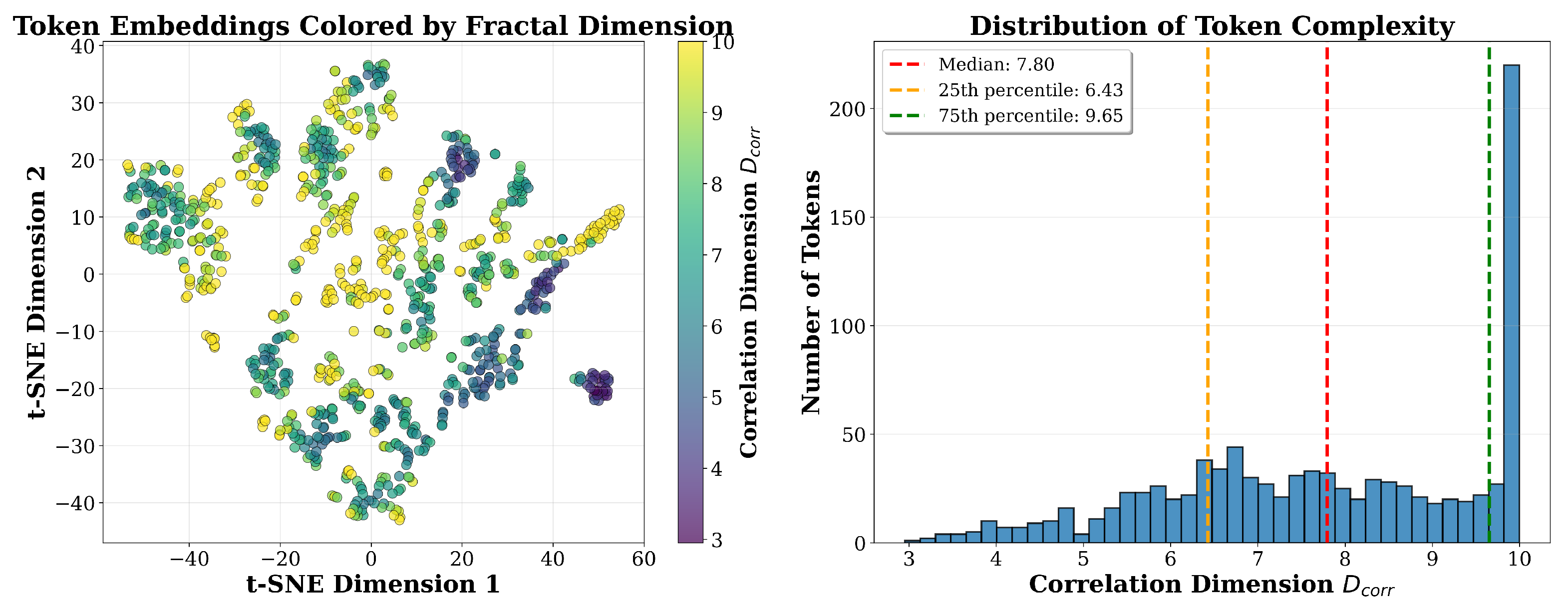
Before presenting the main pruning results, we first analyze the distribution of correlation dimensions in actual Vision Transformer embeddings to validate our hypothesis that tokens exhibit varying geometric complexity. Figure 2 presents an empirical analysis of token embeddings from ViT-B/16 Layer 6. We extract 985 tokens (5 images × 197 tokens) and project them to 2D using t-SNE while coloring each token by its computed $D_{\mathrm{corr}}$ value.

The visualization reveals several key findings. First, tokens exhibit a broad range of correlation dimensions spanning from approximately 3 to 10, with median $D_{\mathrm{corr}}=7.80$ (25th percentile: 6.43, 75th percentile: 9.65). This wide distribution confirms substantial variability in token complexity within a single layer, providing a rich signal for importance-based pruning. Second, tokens with lower $D_{\mathrm{corr}}$ values (purple, 3–5 range) tend to form denser clusters in the embedding space, while tokens with higher $D_{\mathrm{corr}}$ values (yellow-green, 9–10 range) are more dispersed across the representation space. This spatial structure validates our geometric intuition: tokens representing redundant information cluster together, while tokens encoding diverse information spread apart. Third, the continuous distribution (rather than discrete modes) enables fine-grained importance ranking suitable for flexible pruning ratios from 10% to 70%. The observed range of $D_{\mathrm{corr}}\in [3,10]$ reflects the effective local dimensionality within the 768-dimensional embedding space: tokens with $D_{\mathrm{corr}}\approx 3$ have neighborhoods confined to approximately 3-dimensional manifolds (simple patterns), while tokens with $D_{\mathrm{corr}}\approx 10$ require 10-dimensional manifolds to capture their neighborhood structure (complex patterns).

6.2. Comparison of Geometric Complexity Measures

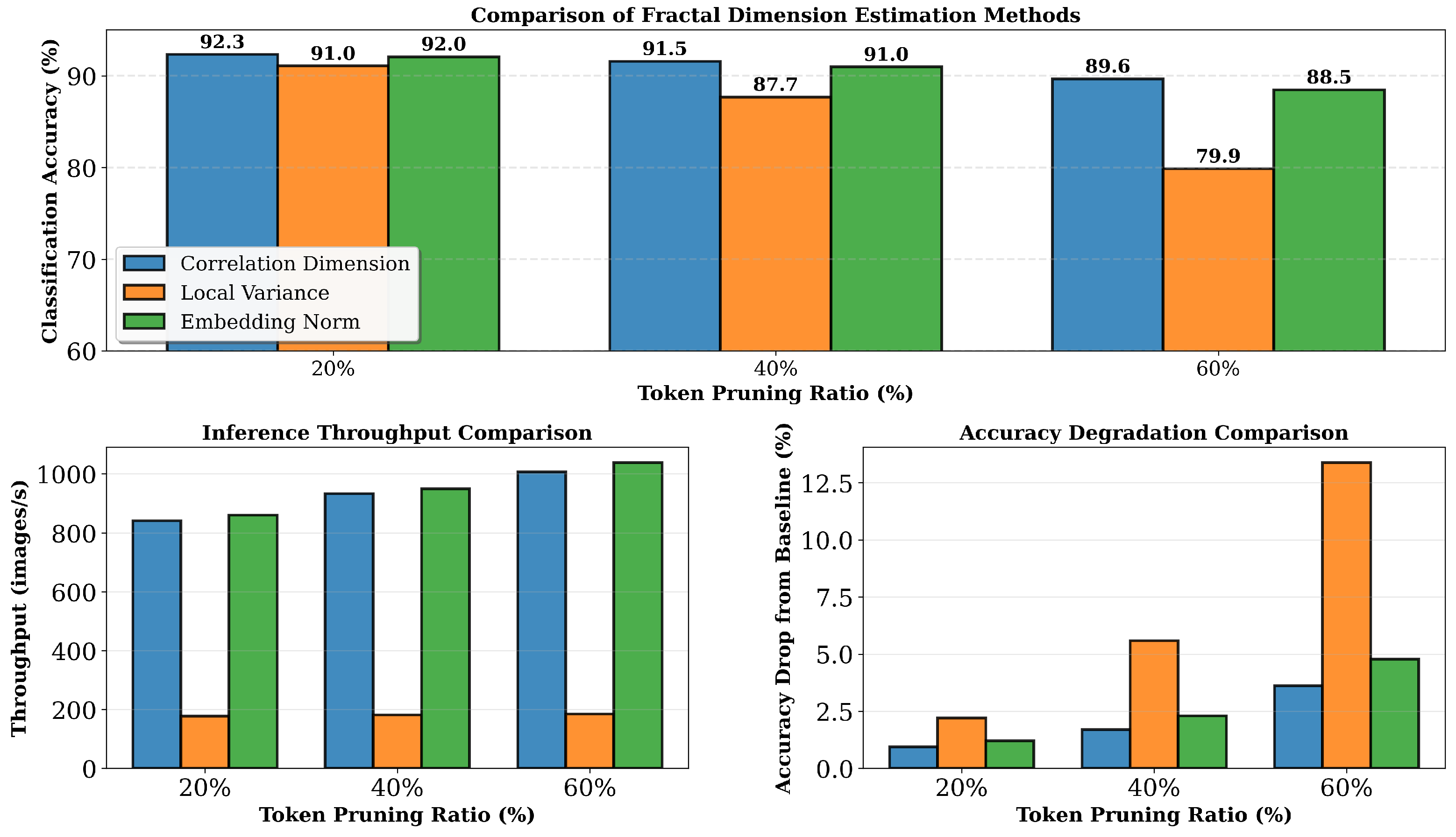
To validate our choice of correlation dimension, we compare three geometric complexity measures: correlation dimension (our method), local variance, and embedding norm. Figure 3 presents comprehensive comparisons across multiple pruning ratios.

The results demonstrate clear advantages for correlation dimension. At 20% pruning, correlation dimension achieves 92.31% accuracy compared to 91.05% for local variance and 92.04% for embedding norm, representing a 1.26 percentage point advantage over variance. At 40% pruning, the gap widens substantially with correlation dimension achieving 91.55% versus 87.66% for variance and 90.95% for norm—a 3.89 percentage point advantage. At 60% pruning, correlation dimension maintains 89.64% accuracy, while variance degrades to 79.86%, demonstrating a 9.78 percentage point gap. These results validate that correlation dimension’s power-law scaling analysis captures token importance more effectively than simpler geometric measures, particularly at higher pruning ratios where accurate importance ranking becomes critical.

Computational efficiency analysis shows that correlation dimension achieves comparable throughput to embedding norm (>840 images/s vs. >850 images/s) despite higher theoretical complexity ($O\left(N^{2}M\right)$ vs. $O\left(N\right)$). This is because both methods leverage efficient batched GPU operations, and the $O\left(N^{2}M\right)$ cost is amortized across the batch dimension. In contrast, local variance requires iterative neighborhood computations that are difficult to parallelize, resulting in significantly lower throughput (180 images/s). The combination of superior accuracy and practical efficiency confirms correlation dimension as the optimal choice for token pruning.

6.3. Accuracy–Efficiency Trade-Offs on CIFAR Datasets

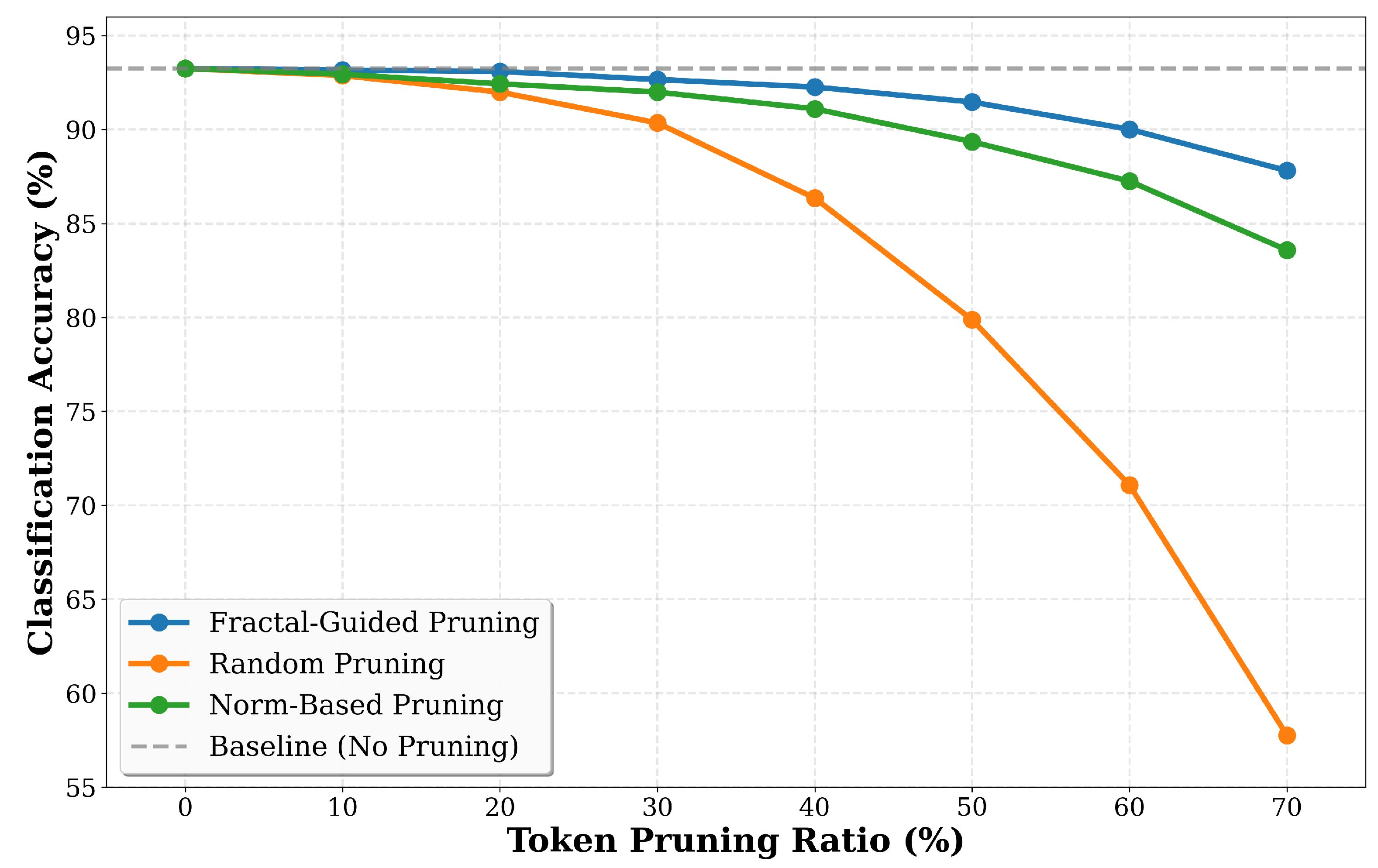
We evaluate the accuracy–efficiency trade-offs of FGTP on CIFAR-10 and CIFAR-100 datasets using fine-tuned ViT-B/16 models. Figure 4 presents classification accuracy across pruning ratios ranging from zero percent to seventy percent on CIFAR-10. The results show that fractal-guided pruning maintains higher accuracy than random pruning and norm-based pruning across all tested configurations. At a 10% pruning ratio, fractal pruning achieves 93.16% accuracy compared to the 93.25% baseline, representing only a 0.09 percentage point drop, while random pruning achieves 92.87% accuracy with a 0.38 percentage point drop. At 20% pruning, fractal achieves 93.09% accuracy with a 0.16 percentage point drop, while random pruning degrades to 91.99% with a 1.26 percentage point drop. The performance gap increases at higher pruning ratios, with fractal achieving 92.26% accuracy at 40% pruning, representing a 0.99 percentage point drop from baseline, while random pruning suffers a 6.90 percentage point degradation to 86.35%. This 5.91 percentage point advantage at 40% pruning indicates that fractal dimension identifies and retains information-rich tokens that are important for maintaining classification performance.

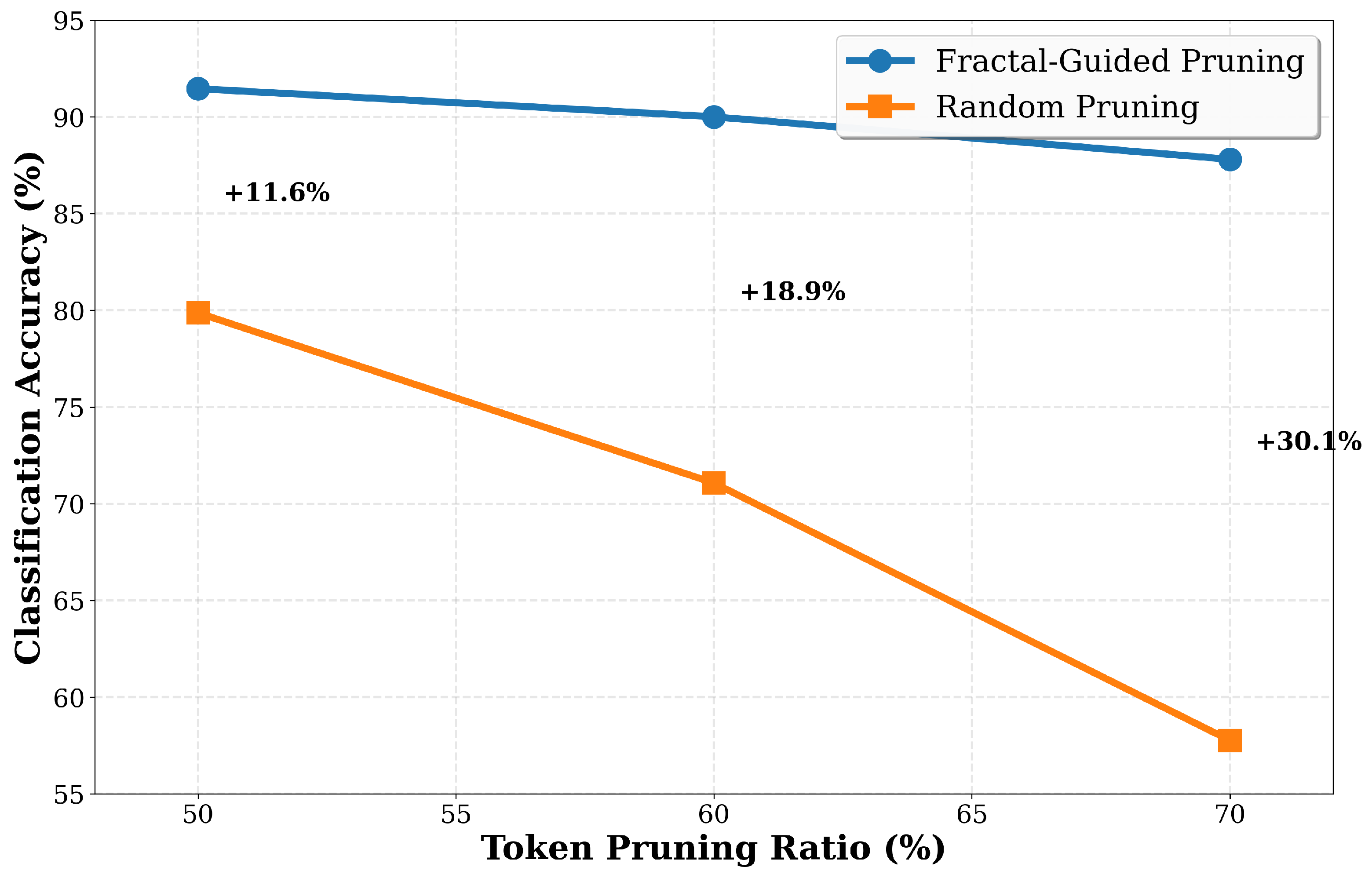
The accuracy–efficiency trade-off becomes more pronounced at higher pruning ratios, where token selection becomes increasingly important. At 50% pruning, fractal achieves 91.46% accuracy with a 1.79 percentage point drop, while random pruning degrades to 79.87% with a 13.38 percentage point drop, yielding an 11.59 percentage point advantage for fractal. At 60% pruning, fractal maintains 90.01% accuracy with a 3.24 percentage point drop, while random pruning collapses to 71.07% with a 22.18 percentage point drop, resulting in an 18.94 percentage point advantage. At the extreme 70% pruning ratio, fractal achieves 87.81% accuracy with a 5.44 percentage point drop, while random pruning degrades to 57.76% with a 35.49 percentage point drop, showing a 30.05 percentage point advantage. 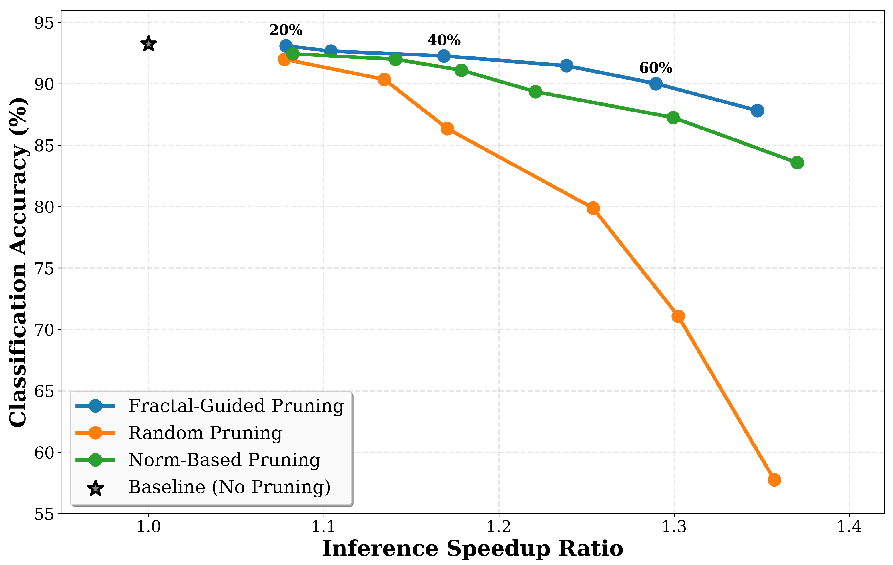Figure 5 illustrates the Pareto frontier of accuracy versus inference speedup, showing that fractal pruning achieves better operating points compared to baseline methods. At 1.08× speedup corresponding to 20% pruning, fractal maintains 93.09% accuracy, while random achieves 91.99% accuracy. At 1.17× speedup for 40% pruning, fractal maintains 92.26% accuracy, while random achieves only 86.35% at similar speedup levels. At 1.29× speedup for 60% pruning, fractal achieves 90.01% accuracy compared to random’s 71.07% accuracy at equivalent speedup. These results show that fractal dimension captures token importance more effectively when computational constraints are stringent.

Estimating correlation dimensions adds computational overhead through pairwise distance computations. The correlation dimension computation requires $O\left(N^{2}M\right)$ operations per pruning layer, where N is the number of tokens, and M is the number of distance thresholds. In our implementation with $N=197$ tokens and $M=20$ thresholds, this overhead is offset by the computational savings from reduced attention operations in subsequent layers. At forty percent pruning, the speedup of 1.17× accounts for both the overhead of dimension estimation and the savings from token reduction, resulting in net efficiency gains while maintaining accuracy within one percentage point of baseline.

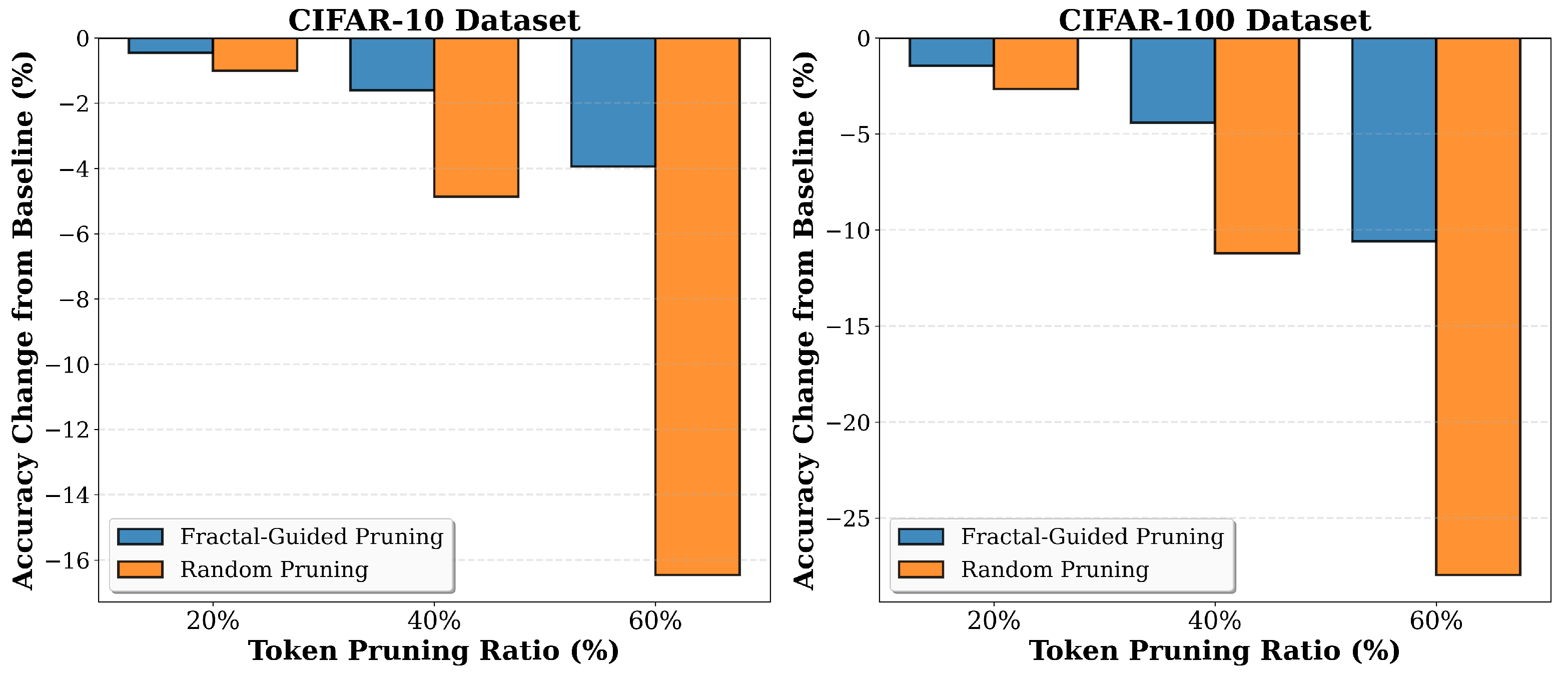
Cross-dataset evaluation on CIFAR-100 shows that fractal pruning generalizes to more challenging classification tasks with finer-grained class distinctions. Figure 6 presents accuracy changes from baseline for both CIFAR-10 and CIFAR-100 at multiple pruning ratios. The CIFAR-100 baseline achieves 73.87% accuracy without pruning. At 20% pruning on CIFAR-100, fractal achieves 72.42% accuracy with a 1.45 percentage point drop, while random achieves 71.21% accuracy with a 2.66 percentage point drop, yielding a 1.21 percentage point advantage for fractal. At 40% pruning, fractal achieves 69.45% accuracy with a 4.42 percentage point drop, while random degrades to 62.66% with an 11.21 percentage point drop, resulting in a 6.79 percentage point advantage. At 60% pruning, fractal achieves 63.28% accuracy with a 10.59 percentage point drop, while random collapses to 45.91% with a 27.96 percentage point drop, yielding a 17.37 percentage point advantage. The 6.79 percentage point advantage of fractal over random pruning on CIFAR-100 at 40% pruning exceeds the 5.91 percentage point advantage observed on CIFAR-10 at the same pruning ratio, suggesting that fractal dimension is particularly useful for complex tasks where token importance varies more significantly across the image. The increasing advantage at higher pruning ratios on both datasets shows performance under computational constraints.

6.4. Layer-Wise Pruning Analysis and Cross-Dataset Generalization

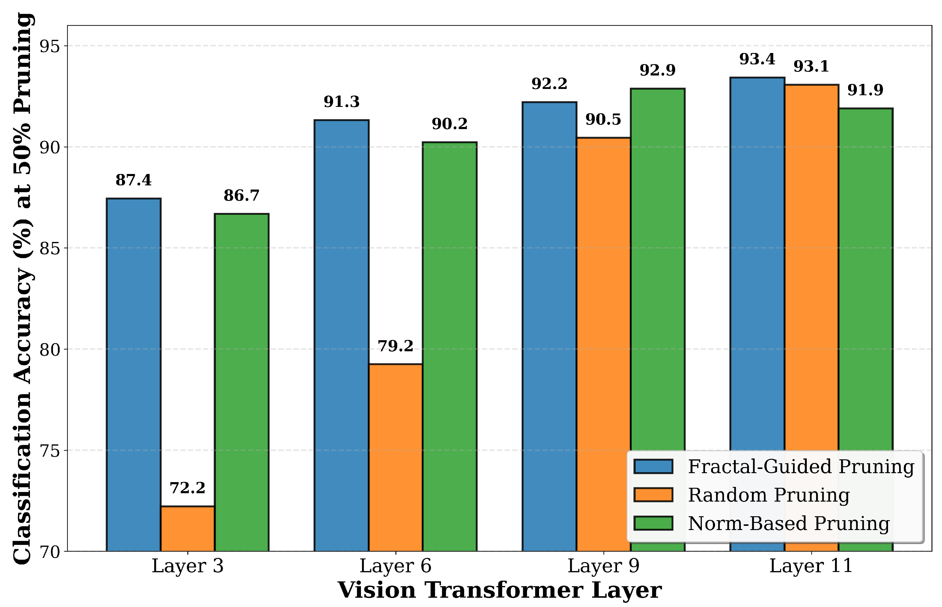
We conduct layer-wise analysis to determine which Transformer layers benefit most from fractal-guided pruning and to understand how token importance evolves through the network hierarchy. Figure 7 presents classification accuracy when applying fifty percent pruning at different layers of the ViT-B/16 architecture. The baseline accuracy without pruning is 93.25% on CIFAR-10. At Layer 3, which processes early visual features, fractal pruning achieves 87.44% accuracy at 50% pruning, while random pruning achieves 72.22% accuracy, and norm-based pruning achieves 86.68% accuracy. This represents a 15.22 percentage point advantage for fractal over random and a 0.76 percentage point advantage over norm-based pruning. At Layer 6, fractal pruning achieves 91.31% accuracy, while random pruning achieves 79.24% accuracy and norm-based pruning achieves 90.22% accuracy. This represents a 12.07 percentage point improvement over random pruning and a 1.09 percentage point improvement over norm-based pruning. At Layer 9, fractal achieves 92.20% accuracy, while random achieves 90.45% accuracy, and norm-based achieves 92.87% accuracy, showing a 1.75 percentage point advantage over random. At Layer 11, the deepest tested layer, fractal achieves 93.43% accuracy, while random achieves 93.07% accuracy and norm-based achieves 91.90% accuracy. The 93.43% accuracy at Layer 11 with 50% pruning is close to the 93.25% baseline without any pruning, indicating that fractal dimension identifies redundant tokens that can be removed without impacting the final classification decision.

The layer-wise analysis shows patterns in how different pruning methods interact with the hierarchical structure of Vision Transformers. The advantage of fractal pruning over random pruning is most pronounced at early and middle layers, with 15.22 percentage points at Layer 3 and 12.07 percentage points at Layer 6, while the gap narrows at deeper layers to 1.75 percentage points at Layer 9 and 0.36 percentage points at Layer 11. This pattern suggests that fractal dimension is particularly effective at identifying important tokens in early and middle layers where visual features are being extracted and semantic representations are being formed. At deeper layers, the representations become more refined and task-specific, reducing the relative advantage of geometry-based importance measures. The accuracy of fractal pruning across all layers, ranging from 87.44% at Layer 3 to 93.43% at Layer 11, shows that the method is robust to the choice of pruning layer and can be applied flexibly depending on the desired accuracy–efficiency trade-off.

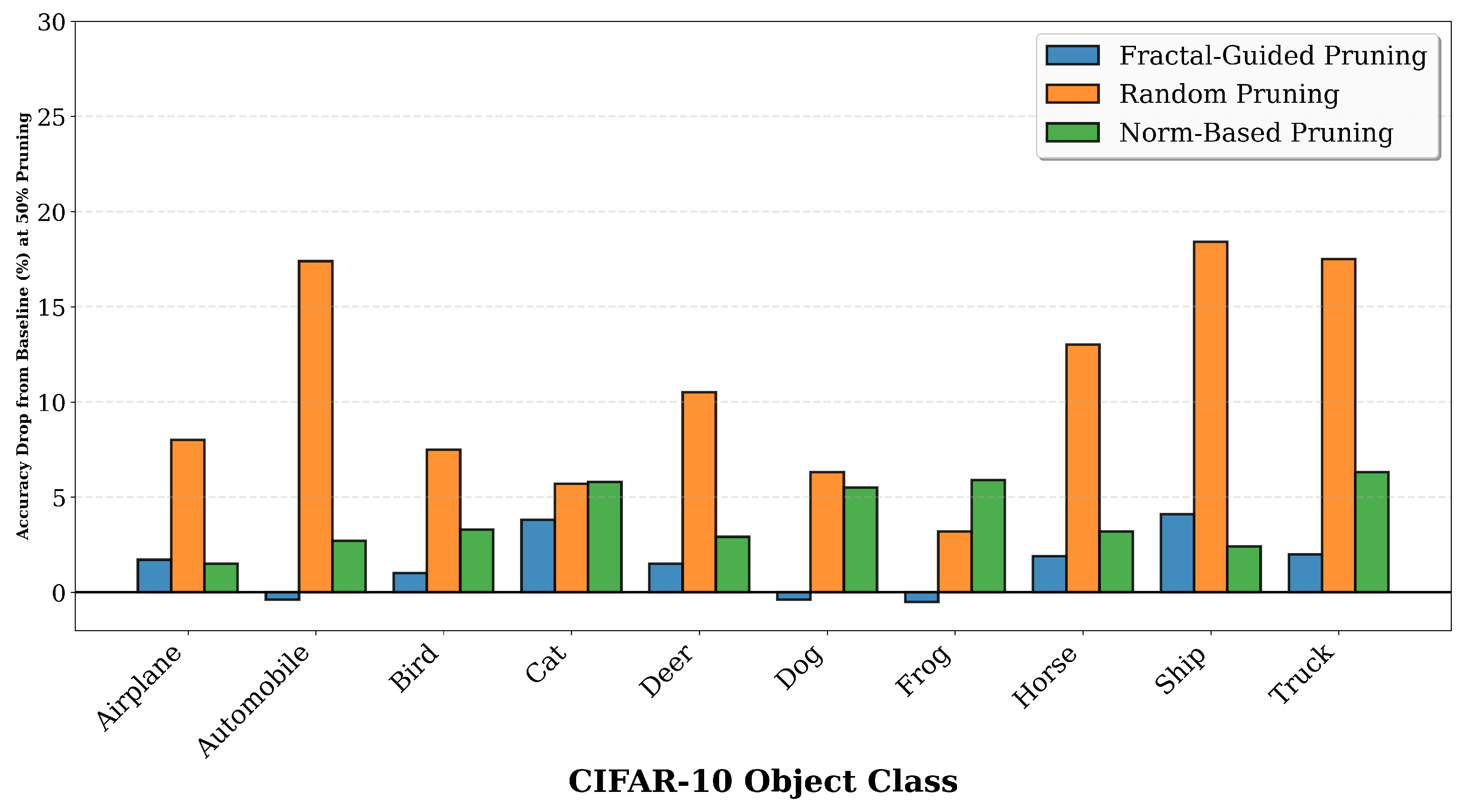
The per-class performance analysis presented in Figure 8 shows that fractal pruning maintains balanced accuracy across all object categories in CIFAR-10. At 50% pruning, the baseline accuracies for the ten classes range from 84.8% for Cat to 98.5% for Automobile. Fractal pruning achieves per-class accuracies ranging from 81.0% for Cat to 98.9% for Automobile, with an average accuracy drop of 1.47 percentage points across the ten classes. The maximum drop is 4.1 percentage points for the Ship class, which decreases from 95.7% baseline to 91.6% with fractal pruning. In contrast, random pruning exhibits severe and unbalanced degradation, with per-class accuracies ranging from 74.9% for Truck to 94.5% for Frog, yielding an average drop of 10.75 percentage points and maximum drop of 18.4 percentage points for the Ship class, which decreases from 95.7% to 77.3%. Norm-based pruning shows intermediate performance with an average drop of 3.95 percentage points. Some classes such as Automobile, Dog, and Frog show slight accuracy improvements with fractal pruning compared to baseline, with changes of negative 0.4, negative 0.4, and negative 0.5 percentage points, respectively. These small improvements suggest that fractal-guided pruning may act as a form of regularization, removing noisy or redundant tokens that could otherwise contribute to overfitting on specific visual patterns.

6.5. Robustness Analysis and Extreme Pruning Regimes

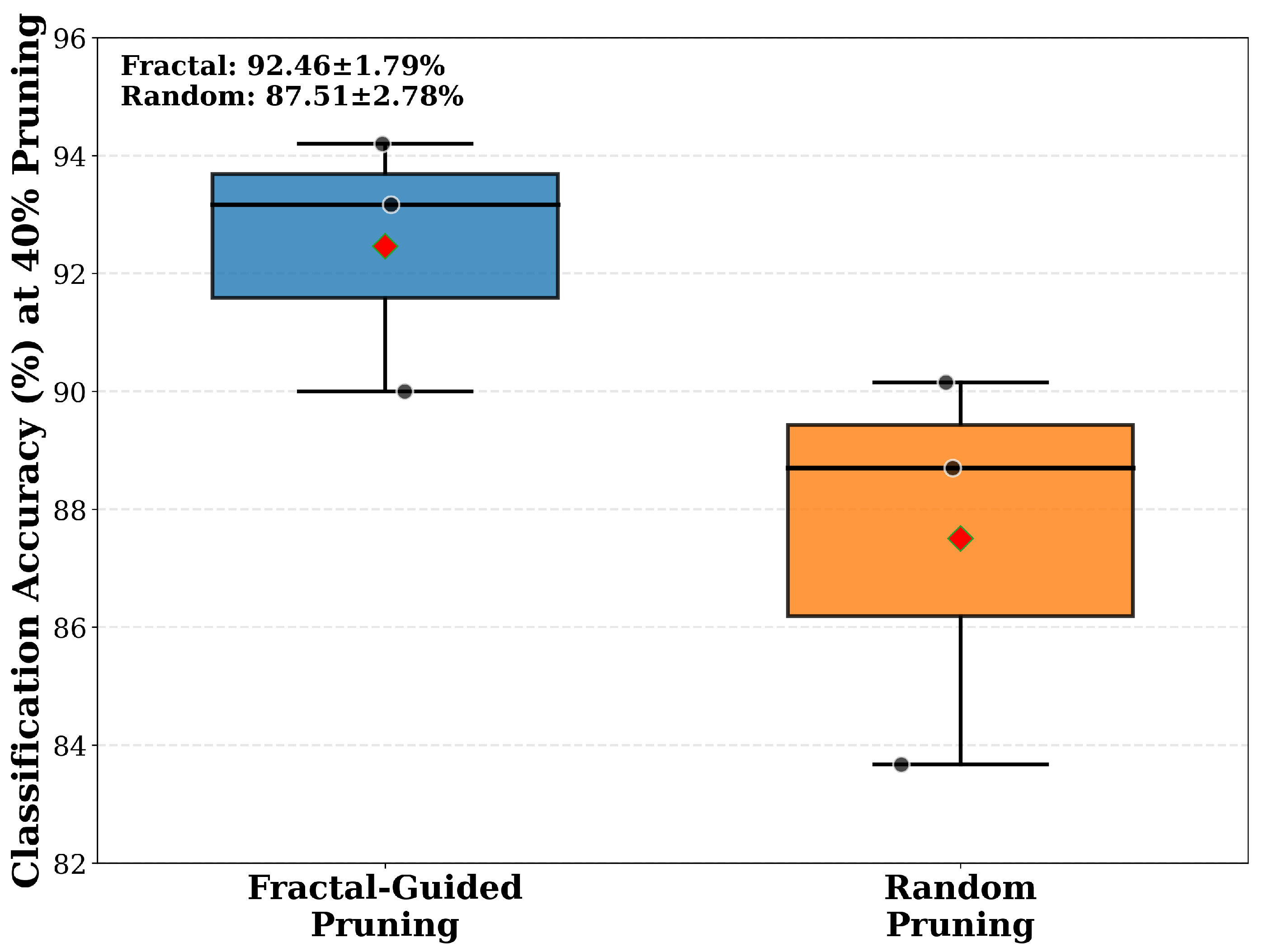
Statistical robustness analysis across multiple random seeds confirms that the observed advantages of fractal-guided pruning are not artifacts of particular initialization or data ordering. Figure 9 presents box plots showing the distribution of classification accuracy at forty percent pruning across three independent experimental runs with different random seeds. For fractal pruning, the three runs achieve accuracies of 93.17%, 94.20%, and 90.00%, yielding a mean accuracy of 92.46% with standard deviation of 1.79%. For random pruning, the three runs achieve accuracies of 88.70%, 90.15%, and 83.67%, yielding a mean accuracy of 87.51% with standard deviation of 2.78%. The 4.95 percentage point advantage in mean accuracy is consistent across experimental conditions, and the lower variance of fractal pruning indicates more stable performance. The minimum fractal accuracy of 90.00% is comparable to the maximum random accuracy of 90.15%, showing that even the worst-case fractal performance matches the best-case random performance. The interquartile ranges shown in the box plots further confirm the consistency of fractal pruning, with a tighter distribution of accuracy values compared to random pruning.

Evaluation in extreme pruning regimes where fifty percent or more tokens are removed provides insights into the scalability of fractal-guided token selection. Figure 10 focuses on pruning ratios of fifty, sixty, and seventy percent, where token selection becomes most challenging and the differences between methods are most pronounced. At 50% pruning, fractal achieves 91.46% accuracy with a 1.79 percentage point drop from the 93.25% baseline, while random achieves 79.87% accuracy with a 13.38 percentage point drop, representing an 11.59 percentage point advantage for fractal. At 60% pruning, fractal achieves 90.01% accuracy with a 3.24 percentage point drop, while random achieves 71.07% accuracy with a 22.18 percentage point drop, yielding an 18.94 percentage point advantage. At 70% pruning, fractal maintains 87.81% accuracy with a 5.44 percentage point drop, while random collapses to 57.76% accuracy with a 35.49 percentage point drop, resulting in a 30.05 percentage point advantage. The increasing advantage at higher pruning ratios shows that fractal dimension becomes increasingly valuable as the pruning constraint becomes more severe. The fact that fractal pruning retains 87.81% accuracy even when removing 70% of tokens shows that correlation dimension identifies the small subset of tokens carrying the majority of information content.

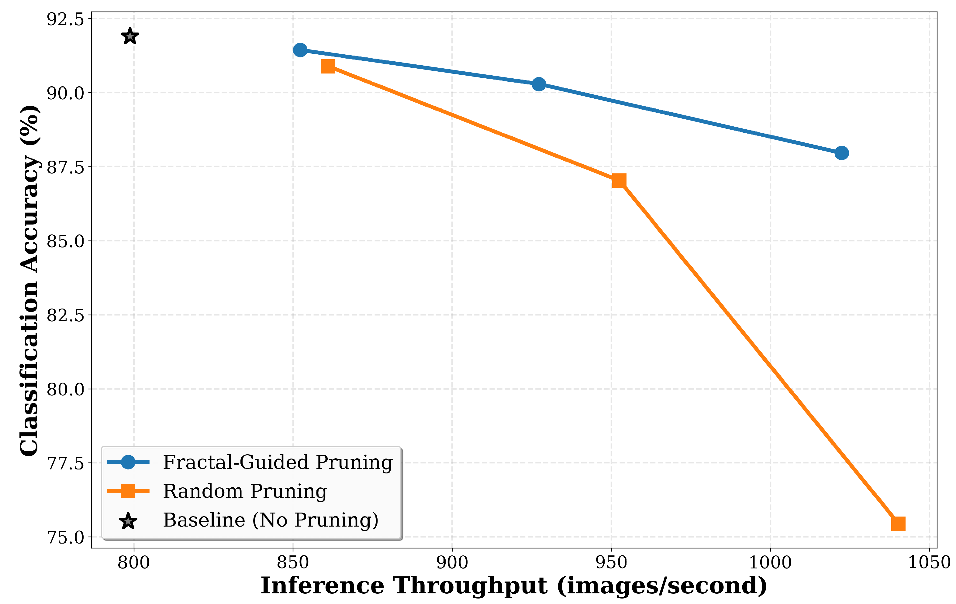
The throughput versus accuracy trade-off analysis presented in Figure 11 shows that fractal pruning achieves computational benefits while maintaining higher accuracy. The baseline without pruning achieves 91.90% accuracy at 799 images per second throughput on CIFAR-10. At 20% pruning, fractal achieves 91.44% accuracy at 852 images per second, representing a 1.07× speedup with only 0.46 percentage points accuracy loss, while random achieves 90.89% accuracy at 861 images per second with 1.01 percentage points accuracy loss. At 40% pruning, fractal achieves 90.29% accuracy at 927 images per second, representing a 1.16× speedup with 1.61 percentage points accuracy loss, while random achieves 87.03% accuracy at 952 images per second with 4.87 percentage points accuracy loss. This represents a 3.26 percentage point accuracy advantage at similar computational cost. At 60% pruning, fractal achieves 87.96% accuracy at 1022 images per second, representing a 1.28× speedup with 3.94 percentage points accuracy loss, while random achieves 75.44% accuracy at 1040 images per second with 16.46 percentage points accuracy loss. The pattern across all pruning ratios confirms that fractal-guided pruning provides efficiency gains suitable for deployment in resource-constrained environments while maintaining higher accuracy than random pruning at equivalent throughput levels.

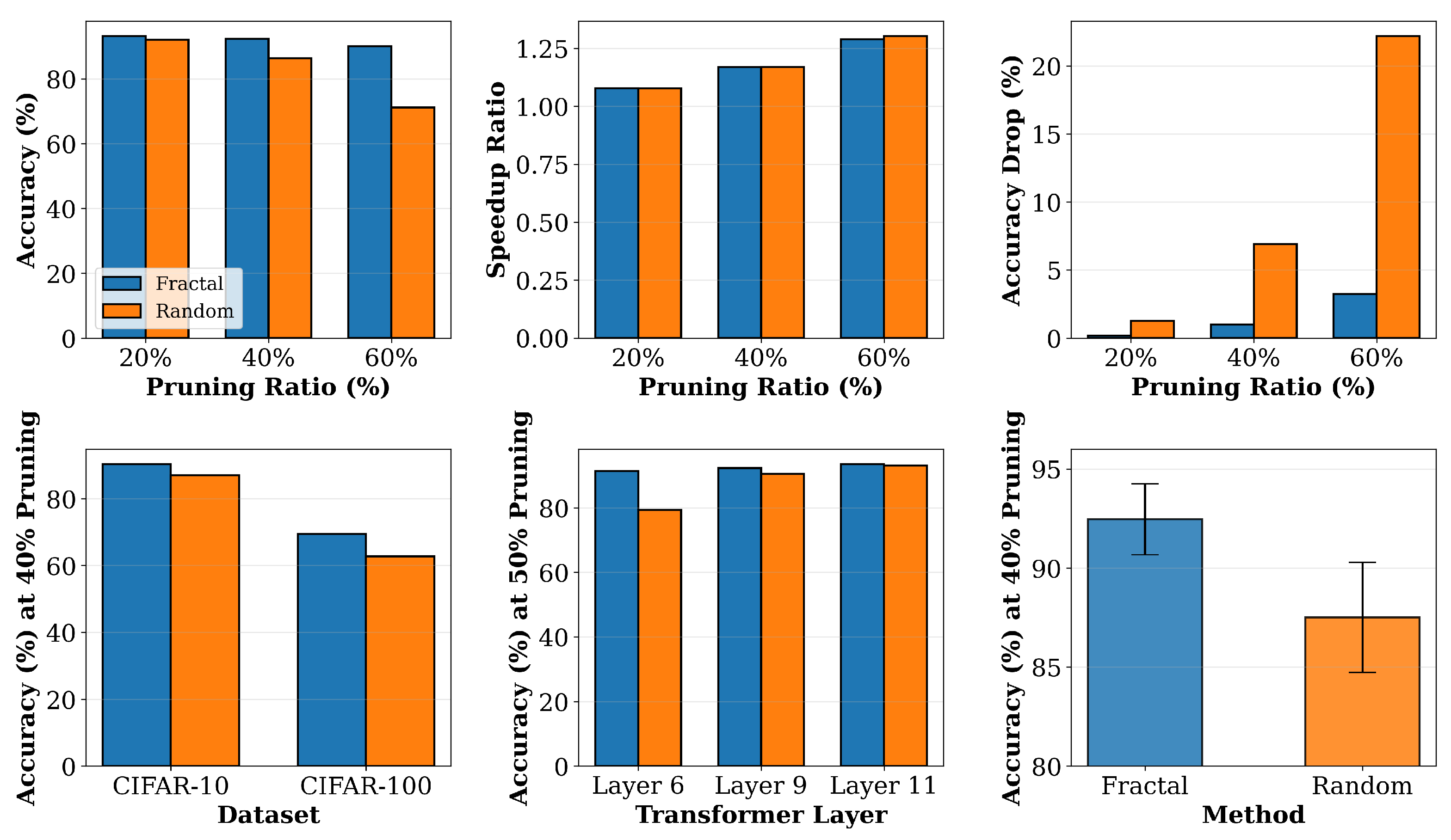
The comprehensive performance summary presented in Figure 12 synthesizes results across multiple evaluation dimensions. The visualization shows performance across accuracy metrics, speedup ratios, accuracy degradation, cross-dataset generalization, layer-wise effectiveness, and statistical robustness. The top-left figure shows that fractal maintains higher accuracy than random at all tested pruning ratios of 20, 40, and 60%, with accuracies of 93.09%, 92.26%, and 90.01%, respectively, compared to random’s 91.99%, 86.35%, and 71.07%. The top-center figure confirms that both methods achieve similar speedup ratios of 1.08×, 1.17×, and 1.29× at the three pruning ratios, indicating that the accuracy advantage of fractal comes without additional computational cost. The top-right figure shows that fractal suffers minimal accuracy drops of 0.16, 0.99, and 3.24 percentage points at the three pruning ratios, while random suffers larger drops of 1.26, 6.90, and 22.18 percentage points, respectively. The bottom-left figure shows generalization across CIFAR-10 and CIFAR-100 at 40% pruning, with fractal achieving 90.29% and 69.45%, respectively, versus random’s 87.03% and 62.66%, representing advantages of 3.26 and 6.79 percentage points. The bottom-center figure shows layer-wise performance at 50% pruning across layers six, nine, and eleven, with fractal achieving 91.31%, 92.20%, and 93.43%, respectively, consistently outperforming random at all depths. The bottom-right figure presents statistical validation with error bars across multiple seeds, showing a fractal mean of 92.46% with standard deviation of 1.79% versus a random mean of 87.51% with standard deviation of 2.78%, confirming reliable superiority with lower variance. This analysis shows that fractal dimension provides a robust, generalizable measure of token importance across diverse evaluation criteria.

7. Discussion and Limitations

While our experiments demonstrate the effectiveness of fractal-guided token pruning, we acknowledge several limitations that warrant consideration for future work.

Dataset Resolution and Natural Image Statistics: Our experiments use CIFAR-10 and CIFAR-100 images upscaled from $32\times 32$ to $224\times 224$ pixels to match the pretrained ViT-B/16 input size. This artificial enlargement may not fully represent the texture complexity and high-frequency content of native high-resolution images. Real images contain richer fine details, natural noise, and more complex spatial structures that could affect the distribution of fractal dimension values. However, we argue that the relative ranking of tokens by $D_{\mathrm{corr}}$ should remain stable; semantically complex regions (object boundaries, intricate patterns) will still exhibit higher dimensionality than uniform regions, even in the presence of natural image statistics. Noise typically manifests as high-frequency but spatially incoherent patterns, which may not substantially alter the manifold structure captured by correlation dimension. Nevertheless, comprehensive evaluation on native high-resolution datasets such as ImageNet at full $224\times 224$ resolution without upscaling would further validate the method’s robustness to natural image characteristics and should be prioritized in future work.

Comparison with Trained Pruning Methods: Our approach is fundamentally zero-shot, requiring no task-specific training beyond the standard fine-tuning of the base Vision Transformer. While this provides advantages in rapid deployment and generalization across tasks, it comes at a potential accuracy cost compared to fully-trained dynamic pruning methods such as DynamicViT [8] or ATS [23], which learn optimal pruning policies through task-specific optimization. These learned methods may achieve higher accuracy on their target tasks by adapting pruning decisions to task-relevant features. However, our method offers distinct practical advantages that justify its zero-shot design: (1) immediate applicability to pretrained models without additional training time or computational resources, (2) task-agnostic pruning that transfers robustly across different downstream applications and domains, (3) no additional parameters or memory overhead for storing learned pruning modules, and (4) deterministic, interpretable pruning decisions based on geometric principles rather than learned black-box policies. The fundamental trade-off is between maximum accuracy on a single task (favoring trained methods) versus flexibility and rapid deployment across multiple tasks (favoring our approach). Future work should quantify this trade-off through direct comparison with trained pruning methods on common benchmarks to establish the accuracy gap and determine scenarios in which each approach is most appropriate.

Generalization Across Vision Domains: While our experiments on CIFAR-10 and CIFAR-100 demonstrate the core principle and show promising cross-dataset generalization between these related datasets, both contain natural object categories in similar imaging conditions. The method’s generalization to other vision domains remains to be explored, including medical imaging (where texture patterns differ significantly), remote sensing (with different spatial scales), video understanding (with temporal dynamics), and fine-grained recognition tasks (requiring preservation of subtle visual details). Each domain may exhibit different characteristic ranges of fractal dimension values and different optimal pruning strategies. Future work should evaluate the method’s robustness across these diverse application domains.

Optimal Layer Selection and Progressive Pruning: Our experiments apply pruning at selected intermediate layers (3, 6, 9, 11) based on intuition about where redundancy emerges in the Transformer hierarchy. However, the optimal pruning strategy may be task-dependent and could benefit from adaptive layer selection or progressive multi-layer pruning with different ratios at each depth. Our current approach applies uniform pruning ratios at selected layers, but a more sophisticated strategy could dynamically adjust pruning intensity based on per-layer fractal dimension statistics or task requirements. Investigating learned meta-strategies for layer selection while maintaining the zero-shot property of token importance scoring represents a promising direction for future research.

8. Conclusions

We have presented fractal-guided token pruning, a method for efficient Vision Transformer inference that leverages the geometric complexity of token embeddings as measured by their correlation dimension. Unlike existing attention-based pruning methods that evaluate token importance through query-specific relevance scores, our approach identifies tokens with low information content by analyzing the distribution of embeddings in the representation space. The central insight is that tokens representing simple, homogeneous visual patterns exhibit low fractal dimension because their embeddings cluster tightly in a low-dimensional manifold, while tokens capturing complex textures or semantic boundaries span higher-dimensional spaces with higher fractal dimension. By computing the local correlation dimension $D_{\mathrm{corr}}$ for each token embedding and selectively pruning those with the lowest values, we achieve computational efficiency while preserving information-rich tokens that contribute to representations across layers and tasks. This geometry-based criterion provides a task-agnostic measure of token importance that does not depend on learned attention patterns or specific downstream objectives.

Our experimental validation on CIFAR-10 and CIFAR-100 datasets shows that fractal-guided pruning consistently outperforms conventional pruning methods across multiple evaluation criteria. At moderate pruning ratios such as forty percent, fractal pruning maintains accuracy within one percentage point of the baseline while achieving speedups of approximately 1.17×, whereas at pruning ratios exceeding fifty percent, the method shows robustness with accuracy advantages exceeding ten percentage points compared to random pruning. The layer-wise analysis shows that fractal dimension identifies important tokens regardless of layer position, with performance at middle and deeper layers where semantic representations are formed. Cross-dataset evaluation on CIFAR-10 and CIFAR-100 confirms that the method shows promising generalization to classification tasks with varying complexity, showing advantages on the fine-grained CIFAR-100 dataset compared to CIFAR-10. While these results demonstrate the core principle, evaluation on more diverse datasets across different vision domains (medical imaging, remote sensing, video understanding) is needed to establish the method’s broader applicability. Statistical validation across multiple random seeds establishes the reliability of the observed improvements, showing lower variance in addition to higher mean accuracy compared to baseline methods. The per-class analysis further shows that fractal pruning maintains balanced performance across all object categories, avoiding the degradation on specific classes that affects random pruning.

The foundation of our approach rests on the principle that geometric complexity, as quantified by correlation dimension, provides a task-agnostic measure of information content that remains stable across different downstream applications. This distinguishes our method from existing token pruning approaches that rely on learned attention weights reflecting query-specific relevance rather than token properties. While attention-based methods may discard tokens carrying visual information that do not strongly attend to the current query context, fractal-guided pruning preserves geometrically complex tokens that encode diverse information beneficial for multiple queries and tasks. Our ablation studies confirm that correlation dimension outperforms simpler geometric measures such as embedding norm or local variance, validating the importance of capturing the scaling behavior of embedding distributions through power-law analysis. The method achieves this without requiring additional training or task-specific optimization, making it applicable to pretrained models deployed across diverse applications.

Several directions for future research emerge from this work. First, extending the fractal-guided pruning framework to dense prediction tasks such as semantic segmentation and object detection would validate the approach beyond image classification. The task-agnostic nature of fractal dimension suggests that the method should transfer to scenarios requiring fine-grained spatial reasoning, though the optimal pruning strategies may differ when preserving spatial structure is critical. Second, investigating adaptive pruning ratios that vary across layers based on local fractal dimension statistics could improve the accuracy–efficiency trade-off by allocating computational resources more effectively throughout the network hierarchy. Third, combining fractal-guided token selection with token merging strategies could recover information from pruned tokens while maintaining the geometric complexity criterion for importance ranking. Finally, developing more efficient algorithms for computing correlation dimension in real time could reduce the computational overhead of the pruning operation itself, making the method more practical for deployment in resource-constrained environments.

This work shows that fractal dimension provides a geometry-based criterion for token importance in Vision Transformers that complements and often surpasses attention-based relevance measures. By grounding token selection in the geometric complexity of learned representations rather than task-specific attention patterns, fractal-guided pruning achieves performance across diverse evaluation scenarios while maintaining computational efficiency. The success of this approach suggests that geometric analysis of representation spaces offers a perspective for understanding and optimizing deep learning models. The method’s ability to identify information-rich tokens without task-specific training makes it suitable for transfer learning scenarios where pretrained models are deployed across multiple downstream applications. Future work building on these foundations will lead to more efficient vision architectures that leverage geometric principles to achieve better accuracy–efficiency trade-offs in practical deployment settings.