Article

Computational and Parameter-Sensitivity Analysis of Dual-Order Memory-Driven Fractional Differential Equations with an Application to Animal Learning

1
School of Software, Northwestern Polytechnical University, 127 West Youyi Road, Beilin District, Xi’an 710072, China
2
Department of Software and Computing Systems, University of Alicante, 03690 Alicante, Spain
3
Department of Applied Mathematics, University of Alicante, 03690 Alicante, Spain
4
Department of Mathematics, Faculty of Sciences, University of Ostrava, 70103 Ostrava, Czech Republic
5
Centre for Wireless Technology, CoE for Intelligent Network, Faculty of Artificial Intelligence & Engineering, Multimedia University, Persiaran Multimedia, Cyberjaya 63100, Selangor, Malaysia
*
Authors to whom correspondence should be addressed.
Fractal Fract. 2025, 9(10), 664; https://doi.org/10.3390/fractalfract9100664
Submission received: 3 September 2025 / Revised: 2 October 2025 / Accepted: 13 October 2025 / Published: 16 October 2025

Abstract

Fractional differential equations are used to model complex systems where present dynamics depend on past states. In this work, we study a linear fractional model with two Caputo orders that captures long-term memory together with short-term adaptation. The existence and uniqueness of solutions are established using Banach and Krasnoselskii’s fixed-point theorems. A parameter study isolates the roles of the fractional orders and coefficients, yielding an explicit stability region in the ( α , β ) –plane via computable contraction bounds. For computation, we implement the Adams–Bashforth–Moulton (ABM) and fractional linear multistep (FLM) methods, comparing accuracy and convergence. As an application, we model animal learning in which proficiency evolves under memory effects and pulsed stimuli. The results quantify the impact of feedback timing on trajectories within the admissible region, thereby illustrating the suitability of dual-order fractional models for memory-driven behavior.

1. Introduction

Differential equations serve as fundamental tools in mathematical modeling, providing a systematic framework for describing dynamic processes in natural and applied sciences. These equations express the relationship between a function and its derivatives, capturing how quantities evolve over time or space. Their applications span multiple disciplines, including physics, engineering, biology, and economics, where they model phenomena such as fluid dynamics, population growth, heat transfer, and biochemical reactions (see [1,2]). In engineering, differential equations play a crucial role in system design, control theory, and signal processing, while in biological sciences, they are used to study disease spread and ecological interactions (for more detail, see [3,4,5]).
Ordinary differential equations traditionally describe systems governed by local interactions, where future states depend only on present conditions and instantaneous changes. However, many real-world processes exhibit nonlocal memory effects, requiring more advanced formulations beyond classical ODEs (see [6,7]). The predictive power of differential equations makes them indispensable in understanding complex systems and advancing technological developments. Their ability to model intricate relationships is essential for both theoretical research and practical applications, guiding innovations in fields such as aerodynamics [8], electromagnetism [9], and material science [10]. As mathematical modeling continues to evolve, differential equations remain at the core of scientific inquiry, facilitating deeper insights into natural and engineered systems (see [11,12,13]).
In behavioral neuroscience, the dynamics of learning and memory retention have been analyzed using ODEs. Specifically, the model introduced in [14,15] captures the response rates of rats subjected to fluctuating shock conditions, without incorporating complex behavioral requirements such as maze navigation. This model is defined by the following equation:
x ( t ) = x ( t 0 ) μ t 0 t x ( ϑ ) σ t ϑ d ϑ ,
where x ( t ) represents the shock response rate at time t, μ is a parameter, and σ is a positive effectiveness function. The term t 0 t x ( ϑ ) σ ( t ϑ ) d ϑ accounts for the accumulated effect of past shocks at time t, weighted by σ .
Experimental findings indicate that memory retention exhibits an exponential decay pattern [16]. Thus, choosing σ ( s ) = exp ( s / τ ) appropriately models this decay, where τ > 0 represents the characteristic memory duration. Substituting this function into Equation (1) yields
x ( t ) = x ( t 0 ) μ exp t τ t 0 t x ( ϑ ) exp ϑ τ d ϑ .
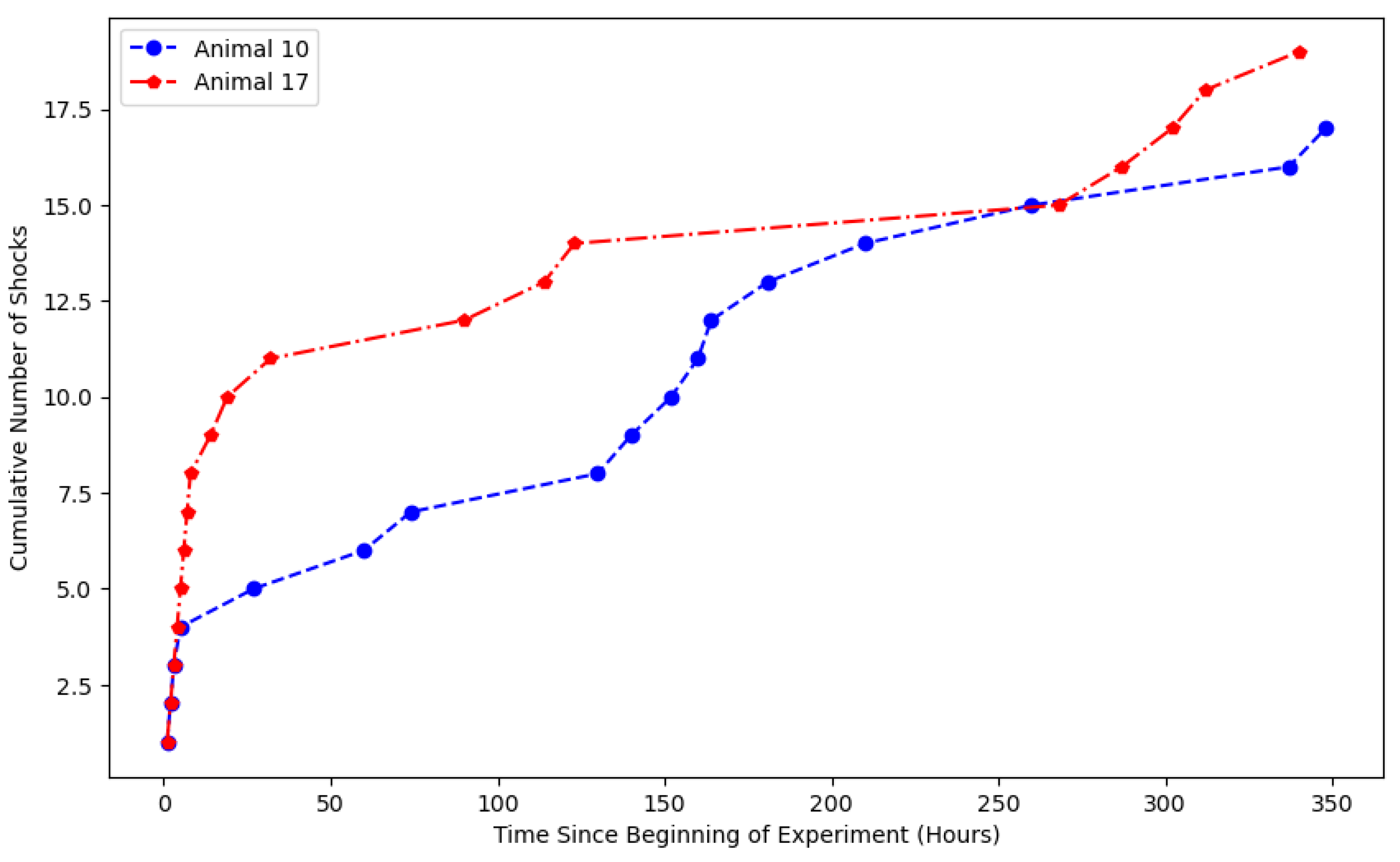
Here, the integral represents memory accumulation, modulated by exponential decay. The initial response rate x ( t 0 ) reflects the tendency of reaction to shocks, while the integral term encapsulates the gradual decline in response due to learning. This formulation successfully explains experimentally observed behavioral trends, including response attenuation over time and occasional resurgence due to forgetting (see Figure 1 and Figure 2).
By differentiating both sides with respect to t, model (2) can be transformed into the following nonhomogeneous second-order ODE:
x ( t ) + 1 τ x ( t ) + μ x ( t ) = 1 τ x t 0 , τ > 0 .
While classical ODEs provide effective models for many dynamical systems, they inherently lack the ability to incorporate memory effects, which are fundamental in describing processes influenced by historical states. This limitation makes ODEs inadequate for capturing dynamics in various real-world applications, including the following:
  • Memory-dependent materials, where the stress–strain relationship is influenced by prior deformations [17].
  • Anomalous diffusion processes, commonly observed in transport through heterogeneous media, deviating from classical Brownian motion [18].
  • Biological and artificial intelligence models, where adaptive behavior arises from accumulated past inputs [19].
  • Neural dynamics and population growth models, where historical states exert a long-term influence on system evolution [20].
To address these limitations, we adopt a fractional differential equation (FDE) framework, which extends classical ODEs by allowing non-integer orders and thus models memory and hereditary effects (see [21,22,23,24] and the references therein). Fractional operators capture slowly decaying kernels and scale-dependent responses that integer-order models miss. They also permit distinct time scales within a single linear law, which is essential for separating fast adaptation from slow consolidation. We consider
D t α x ( t ) + 1 τ D t β x ( t ) + μ x ( t ) = 0 , t [ t 0 , T ] ,
with initial conditions
x ( t 0 ) = x 0 , x ( t 0 ) = x 1 .
Here, D t α and D t β are Caputo derivatives of orders 1 < α < 2 and 0 < β < 1 , respectively, with α β > 1 . The inclusion of multiple fractional orders accounts for diverse memory effects, applicable in viscoelasticity, anomalous diffusion, and learning models.
This work investigates fractional models (4) and (5) with two Caputo derivatives of distinct orders to capture memory-dependent dynamics. Existence and uniqueness on a finite interval are obtained by fixed-point arguments (Banach and, in a complementary splitting, Krasnosel’skii). A parameter study quantifies the influence of the fractional orders and coefficients and delineates a stability region in the ( α , β ) plane via computable contraction bounds. For computation, we implement the Adams–Bashforth–Moulton predictor–corrector scheme and a fractional linear multistep method and compare accuracy and convergence. The model is then applied to animal learning, where stimulus timing shapes learning trajectories.
From a biological standpoint, the two Caputo orders encode distinct time scales of memory. The term D t α x with 1 < α < 2 models slow consolidation (long-range retention), whereas the lower-order term 1 τ D t β x with 0 < β < 1 captures fast adaptive updates driven by recent feedback. The parameter τ sets the relative weight of these modes. In this dual-order formulation, the effective memory kernel behaves as a superposition of two power laws, a common surrogate for heterogeneous retention in cognition and behavior. Thus, the pair ( α , β ) separates long-term consolidation from short-term adaptation within a single linear model, while the constraint α β > 1 aligns with the well-posedness regime used in the analysis.
The structure of this paper is as follows. Section 2 introduces the necessary mathematical concepts. The existence and uniqueness results are derived in Section 3, whereas Section 4 focuses on the parameter effects and the construction of the stability region. In the end, we present the application to learning behavior, which is supported by numerical results.

2. Preliminaries

We present essential definitions and fundamental results required for subsequent sections.
Definition 1 
([25]). Let η > 0 and set ξ = η + 1 so that ξ 1 < η < ξ . Assume W C ξ 1 [ 0 , ) , and W ( ξ 1 ) is locally absolutely continuous on [ 0 , ) . The (left-sided) Caputo fractional derivative of order η is
D η W ( s ) = 1 Γ ( ξ η ) 0 s ( s θ ) ξ η 1 W ( ξ ) ( θ ) d θ , s 0 , ( ξ 1 < η < ξ ) .
The (left-sided) Riemann–Liouville fractional integral of order η > 0 is
I η f ( s ) : = 1 Γ ( η ) 0 s ( s θ ) η 1 f ( θ ) d θ , s 0 .
These operators satisfy the identities
D η I η f = f , I η D η W ( s ) = W ( s ) k = 0 ξ 1 W ( k ) ( 0 + ) k ! s k .
The general solution of the homogeneous equation D η W ( v ) = 0 is the polynomial
W ( v ) = δ 0 + δ 1 v + δ 2 v 2 + + δ ξ 1 v ξ 1 ,
with arbitrary constants δ k R for k = 0 , 1 , , ξ 1 .
Now, we present the proof of the following lemma, which will be used in the latter section.
Lemma 1. 
Let x C 1 ( [ t 0 , T ] , R ) satisfy the fractional differential equation
D t α x ( t ) + 1 τ D t β x ( t ) + μ x ( t ) = 0 , t [ t 0 , T ] , x ( t 0 ) = x 0 , x ( t 0 ) = x 1 ,
where D t α and D t β denote Caputo fractional derivatives of orders 1 < α < 2 and 0 < β < 1 , respectively, with α β > 1 . Then, x is a solution to the fractional differential Equation (6) if and only if it satisfies the following integral equation:
x ( t ) = x 0 + x 1 ( t t 0 ) + x 0 τ Γ ( α β + 1 ) t t 0 α β 1 τ Γ ( α β ) t 0 t ( t θ ) α β 1 x ( θ ) d θ μ Γ ( α ) t 0 t ( t θ ) α 1 x ( θ ) d θ .
Proof. 
Assume that x ( t ) solves Equation (6). Apply the Riemann–Liouville integral operator I t α to both sides of
I t α D t α x ( t ) + 1 τ I t α D t β x ( t ) + μ I t α x ( t ) = 0 .
Using the property of the Caputo fractional derivative for α ( 1 , 2 ) and incorporating the initial conditions x ( t 0 ) = x 0 and x ( t 0 ) = x 1 , we get
x ( t ) = x 0 + x 1 ( t t 0 ) 1 τ I t α D t β x ( t ) μ I t α x ( t ) .
For the Caputo fractional derivative D t β x ( t ) with 0 < β < 1 , using the composition property of fractional integrals and derivatives, given by I t α D t β x ( t ) = I t α β x ( t ) , we have
I t α β x ( t ) = 1 Γ ( α β ) t 0 t ( t θ ) α β 1 x ( θ ) d θ .
Similarly, I t α x ( t ) = 1 Γ ( α ) t 0 t ( t θ ) α 1 x ( θ ) d θ . Substituting these into the Equation (8) yields Equation (7).
Conversely, assume that x ( t ) satisfies Equation (7). By using the properties of the fractional differential equation, we can easily recover the FDE given in Equation (6). The initial conditions x ( t 0 ) = x 0 and x ( t 0 ) = x 1 follow directly from evaluating Equation (7) and its first derivative at t = t 0 . The equivalence is thereby established. □
In the sequel, the following well-established results will be utilized.
Theorem 1 
(Banach’s fixed-point theorem [26]). Let ( X , d ) be a complete metric space, and suppose that an operator Z : X X satisfies the contraction condition
d ( Z x , Z y ) k d ( x , y ) , x , y X ,
where 0 k < 1 . Then, Z has a unique fixed point x ˜ X , and for any initial point x 0 X , the sequence of iterates Z n ( x 0 ) converges to x ˜ , i.e.,
Z n ( x 0 ) x ˜ as n .
Theorem 2 
(Krasnoselskii’s fixed-point theorem [27]). Let X be a nonempty, bounded, closed, and convex subset of a Banach space B , and let the operators Z 1 , Z 2 : X B satisfy the following conditions:
1. 
Z 1 k + Z 2 k X , for all k , k X .
2. 
Z 1 is compact and continuous.
3. 
Z 2 is a contraction mapping.
Then, the sum Z 1 + Z 2 has at least one fixed point in X.

3. Analytical Investigation

To establish the well-posedness of solutions for the integral Equation (7) associated with the fractional differential Equation (6), we construct a functional framework that respects both the operators’ characteristics and the solution’s regularity requirements. The presence of Caputo derivatives D t α and D t β with 1 < α < 2 , 0 < β < 1 , and α β > 1 necessitates solutions with enhanced smoothness properties beyond mere continuity. We therefore work within the Banach space
X = C 1 ( [ t 0 , T ] , R ) ,
where C 1 ( [ t 0 , T ] , R ) denotes the set of real-valued functions possessing continuous first derivatives on [ t 0 , T ] . This space is equipped with the composite norm
x C 1 = sup t [ t 0 , T ] | x ( t ) | + sup t [ t 0 , T ] | x ( t ) | ,
which simultaneously controls function values and their rates of change. This dual control proves essential for managing the memory effects inherent in fractional operators. The completeness of ( X , · C 1 ) follows from fundamental results in functional analysis (see [28]).
Lemma 2. 
Assume 1 < α < 2 , 0 < β < 1 , and α β > 1 and let x C 1 ( [ t 0 , T ] , R ) . For t [ t 0 , T ] , define
V α β ( t ) : = t 0 t ( t θ ) α β 1 x ( θ ) d θ , V α ( t ) : = t 0 t ( t θ ) α 1 x ( θ ) d θ .
and then V α β , V α C 1 ( [ t 0 , T ] ) . Moreover, with x : = sup s [ t 0 , T ] | x ( s ) | , for all t [ t 0 , T ] , we have the bounds
| V α β ( t ) | ( t t 0 ) α β α β x , | V α ( t ) | ( t t 0 ) α α x ,
and
| d d t V α β ( t ) | = | t 0 t ( α β 1 ) ( t θ ) α β 2 x ( θ ) d θ | ( t t 0 ) α β 1 x ,
| d d t V α ( t ) | = | t 0 t ( α 1 ) ( t θ ) α 2 x ( θ ) d θ | ( t t 0 ) α 1 x .
This carefully constructed setting provides the necessary foundation for applying fixed-point theorems to prove solution existence and uniqueness. Here is the first result.
Theorem 3. 
Assume 1 < α < 2 , 0 < β < 1 , α β > 1 , τ > 0 , and μ R . Let X = C 1 ( [ t 0 , T ] , R ) be the Banach space endowed with the norm Equation (10). Define Z : X X by
( Z x ) ( t ) = x 0 + x 1 ( t t 0 ) + x 0 τ Γ ( α β + 1 ) ( t t 0 ) α β 1 τ Γ ( α β ) t 0 t ( t θ ) α β 1 x ( θ ) d θ μ Γ ( α ) t 0 t ( t θ ) α 1 x ( θ ) d θ .
if
k : = ( T t 0 ) α β τ Γ ( α β + 1 ) + | μ | ( T t 0 ) α Γ ( α + 1 ) + ( T t 0 ) α β 1 τ Γ ( α β ) + | μ | ( T t 0 ) α 1 Γ ( α ) < 1 ,
Then, we have the following:
1. 
Z is a strict contraction on ( X , · C 1 ) and hence admits a unique fixed point x X .
2. 
This fixed point x is the unique solution of the integral Equation (7) on [ t 0 , T ] .
3. 
Moreover, by the equivalence between the differential and integral formulations, x is the unique solution of the Caputo problem (6) with x ( t 0 ) = x 0 and x ( t 0 ) = x 1 .
Proof. 
The operator Z : X X is well-defined, as both fractional integral terms preserve C 1 -regularity. This follows from standard differentiation properties of fractional integrals (see [29]), ensuring that Z x C 1 t 0 , T , R .
Next, to prove the contraction condition, we let x , y X = C 1 ( [ t 0 , T ] , R ) and write · : = sup t [ t 0 , T ] | · | . Note that x y x y C 1 . The difference between the operator evaluations satisfies
Z x Z y C 1 = sup t [ t 0 , T ] | Z x ( t ) Z y ( t ) | + sup t [ t 0 , T ] | ( Z x ) ( t ) ( Z y ) ( t ) | .
For the function component, we have
| Z x ( t ) Z y ( t ) | 1 τ Γ ( α β ) t 0 t ( t θ ) α β 1 | x ( θ ) y ( θ ) | d θ + | μ | Γ ( α ) t 0 t ( t θ ) α 1 | x ( θ ) y ( θ ) | d θ ( T t 0 ) α β τ Γ ( α β + 1 ) + | μ | ( T t 0 ) α Γ ( α + 1 ) x y .
On the other hand, for the derivative component, we have
| ( Z x ) ( t ) ( Z y ) ( t ) | α β 1 τ Γ ( α β ) t 0 t ( t θ ) α β 2 | x ( θ ) y ( θ ) | d θ + | μ | ( α 1 ) Γ ( α ) t 0 t ( t θ ) α 2 | x ( θ ) y ( θ ) | d θ ( T t 0 ) α β 1 τ Γ ( α β ) + | μ | ( T t 0 ) α 1 Γ ( α ) x y .
Combining these estimates, we obtain
Z x Z y C 1 k x y C 1 ,
where the contraction constant k is given by Equation (12).
By the hypothesis k < 1 , the operator Z is a contraction on ( X , · C 1 ) . Since X is complete, Theorem 1 yields a unique x X with Z x = x . By the equivalence between Equations (6) and (7), this fixed point is the unique solution to both the integral Equation (7) and the fractional differential Equation (6). □
Corollary 1. 
Under the hypotheses of Theorem 3, there exists δ 0 > 0 such that for any T with 0 < T t 0 < δ 0 , the operator Z defined in Equation (11) is a contraction on X = C 1 ( [ t 0 , T ] , R ) . Consequently, the conclusions of Theorem 3 hold on [ t 0 , T ] .
Corollary 2. 
Under the hypotheses of Theorem 3, for any fixed interval [ t 0 , T ] and
| μ | < Γ ( α ) ( 1 ϵ ) ( T t 0 ) α 1 1 + ( T t 0 ) f o r s o m e ϵ > 0 ,
there exists τ 0 > 0 such that for all τ > τ 0 , the operator Z defined in Equation (11) is a contraction on X = C 1 ( [ t 0 , T ] , R ) . Consequently, the conclusions of Theorem 3 hold on [ t 0 , T ] .
Proof. 
From Theorem 3,
k = ( T t 0 ) α β τ Γ ( α β + 1 ) + | μ | ( T t 0 ) α Γ ( α + 1 ) + ( T t 0 ) α β 1 τ Γ ( α β ) + | μ | ( T t 0 ) α 1 Γ ( α ) .
Grouping the τ -dependent terms gives
k ( T t 0 ) α β 1 1 + ( T t 0 ) τ Γ ( α β ) = : k 1 ( τ ) + | μ | ( T t 0 ) α 1 1 + ( T t 0 ) Γ ( α ) = : k 2 .
Given ϵ > 0 , we choose
τ 0 > ( T t 0 ) α β 1 1 + ( T t 0 ) ϵ Γ ( α β ) k 1 ( τ ) < ϵ for all τ > τ 0 .
By the hypothesis on | μ | , we have k 2 < 1 ϵ . Hence, for all τ > τ 0 ,
k k 1 ( τ ) + k 2 < ϵ + ( 1 ϵ ) = 1 ,
So, Z is a contraction on ( X , · C 1 ) . The conclusions of Theorem 3 follow. □
Theorem 4. 
Let X = C 1 ( [ t 0 , T ] , R ) with the norm (10). Assume 1 < α < 2 , 0 < β < 1 , α β > 1 , τ > 0 , and μ R . Define A , B : X X by
( A x ) ( t ) = x 0 + x 1 ( t t 0 ) + x 0 τ Γ ( α β + 1 ) ( t t 0 ) α β μ Γ ( α ) t 0 t ( t θ ) α 1 x ( θ ) d θ , ( B x ) ( t ) = 1 τ Γ ( α β ) t 0 t ( t θ ) α β 1 x ( θ ) d θ .
Set
k ˜ : = ( T t 0 ) α β τ Γ ( α β + 1 ) + ( T t 0 ) α β 1 τ Γ ( α β ) , c A : = | μ | ( T t 0 ) α Γ ( α + 1 ) + | μ | ( T t 0 ) α 1 Γ ( α ) .
Assume k ˜ + c A < 1 and let
C 0 : =   | x 0 |   +   | x 1 | ( T t 0 ) + | x 0 | τ Γ ( α β + 1 ) ( T t 0 ) α β + | x 1 | + | x 0 | τ Γ ( α β ) ( T t 0 ) α β 1 ,
and choose r C 0 1 ( k ˜ + c A ) . Then, on the closed ball Ω : = { x X : x C 1 r } , all hypotheses of Theorem 2 hold for Z 1 = A and Z 2 = B . Hence, Z = A + B admits a fixed point x Ω , which solves Equation (7), and by the equivalence Lemma 1, Equation (6) is also solved.
Proof. 
For x X , both integrals are well-defined. Since α 1 > 0 and α β 1 > 0 , the kernels vanish at the diagonal, so the boundary term at θ = t is zero, and Leibniz’ rule yields
d d t t 0 t ( t θ ) α 1 x ( θ ) d θ = t 0 t ( α 1 ) ( t θ ) α 2 x ( θ ) d θ ,
d d t t 0 t ( t θ ) α β 1 x ( θ ) d θ = t 0 t ( α β 1 ) ( t θ ) α β 2 x ( θ ) d θ .
Because 1 < α < 2 and α β > 1 , the right-hand sides are finite and depend continuously on t (dominated convergence); hence, A x , B x C 1 ( [ t 0 , T ] ) .
For x , y X and · : = sup [ t 0 , T ] | · | , we have
B x B y 1 τ Γ ( α β ) t 0 T ( T θ ) α β 1 d θ x y = ( T t 0 ) α β τ Γ ( α β + 1 ) x y ,
( B x B y ) α β 1 τ Γ ( α β ) t 0 T ( T θ ) α β 2 d θ x y = ( T t 0 ) α β 1 τ Γ ( α β ) x y ,
So B x B y C 1 k ˜ x y k ˜ x y C 1 , i.e., B is a contraction.
If x C 1 r , then x r , and
A x C 0 + | μ | Γ ( α ) t 0 T ( T θ ) α 1 d θ r = C 0 + | μ | ( T t 0 ) α Γ ( α + 1 ) r ,
( A x ) | x 1 | + | x 0 | τ Γ ( α β ) ( T t 0 ) α β 1 + | μ | ( T t 0 ) α 1 Γ ( α ) r ,
Hence, A x C 1 C 0 + c A r . Standard estimates for differences of such integrals (with | x | r and 0 h s γ d s = h γ + 1 / ( γ + 1 ) for γ > 1 ) yield equicontinuity of A x and ( A x ) on bounded sets. Therefore, A is compact by Arzelà–Ascoli theorem [30] and continuous by dominated convergence.
For x , y Ω ,
A x + B y C 1 A x C 1 + B y C 1 C 0 + ( c A + k ˜ ) r .
if k ˜ + c A < 1 and r C 0 / ( 1 ( k ˜ + c A ) ) , then A x + B y C 1 r ; hence, A x + B y Ω . Thus, Theorem 2 applies on Ω with Z 1 = A , Z 2 = B , giving a fixed point x Ω of Z = A + B . This identity is (7), and by equivalence, Lemma 1 x also solves Equation (6). □
As a direct corollary of the contraction estimate in Theorem 3, we obtain the following stability bound (for further details on stability, see [31,32] and the references cited therein).
Corollary 3. 
Let k < 1 be as it is in Theorem 3 and set Δ : = T t 0 . If y C 1 ( [ t 0 , T ] ) satisfies
| D t α y ( t ) + 1 τ D t β y ( t ) + μ y ( t ) | ϕ ( t ) for t [ t 0 , T ] ,
with ϕ L ( [ t 0 , T ] ) (non-negative a.e.), then the unique solution x of (6) and (7) obeys
y x C 1 1 1 k Δ α Γ ( α + 1 ) + Δ α 1 Γ ( α ) ϕ .
In particular, if ϕ δ > 0 , then
y x C 1 δ 1 k Δ α Γ ( α + 1 ) + Δ α 1 Γ ( α ) .
Remark 1. 
Consider the forced problem
D t α x + 1 τ D t β x + μ x = S ( t ) ,
and let S ˜ be a perturbed stimulus with the same initial data as x. Denote Δ S : = S ˜ S L ( [ t 0 , T ] ) and let x ˜ be the corresponding solution. Then,
D t α ( x ˜ x ) + 1 τ D t β ( x ˜ x ) + μ ( x ˜ x ) = Δ S ,
Thus, Corollary 3 applied with y = x ˜ , with x as stated above, and ϕ = | Δ S | yields
x ˜ x C 1 C stab Δ S , C stab : = 1 1 k Δ α Γ ( α + 1 ) + Δ α 1 Γ ( α ) ,
where Δ = T t 0 , and k < 1 is as in Theorem 3. In the learning context, this establishes robustness, namely that bounded perturbations of the feedback (amplitude errors, noise, and unmodeled inputs) yield proportionally bounded changes in the proficiency trajectory.
Example 1. 
Consider the fractional model
D t 1.8 x ( t ) + 1 2 D t 0.5 x ( t ) + 0.1 x ( t ) = 0 , t [ 0 , 0.5 ] ,
i.e., α = 1.8 , β = 0.5 , μ = 0.1 , τ = 2 , t 0 = 0 , and T = 0.5 . The admissibility condition holds:
α β = 1.3 > 1 .
For Theorem 4 (existence), the contraction constant of B is
k ˜ = ( T t 0 ) α β τ Γ ( α β + 1 ) + ( T t 0 ) α β 1 τ Γ ( α β ) 0.62657 < 1 .
The invariance constant is
c A : = | μ | ( T t 0 ) α Γ ( α + 1 ) + | μ | ( T t 0 ) α 1 Γ ( α ) 0.07880 .
Hence, k ˜ + c A 0.70537 < 1 , so all hypotheses of Theorem 4 are satisfied and the problem admits at least one solution on [ 0 , 0.5 ] .
For Theorem 3, the global Lipschitz constant is
k = k ˜ + c A 0.70537 < 1 .
Since k < 1 , Z is a strict contraction, and there is a unique solution to Equation (17). Moreover, the numerical verification of this result using the Picard iteration is illustrated in Figure 3, which demonstrates the iterative convergence of the approximate solution towards the exact solution.
By Corollary 3 and the value k 0.70537 < 1 computed above, problem (17) admits Ulam–Hyers–Rassias stability on [ 0 , 0.5 ] with the explicit bound stated therein.

4. Parameter Sensitivity Analysis

Figure 4 displays the ( α , β ) pairs for which Equations (4) and (5) are well posed on [ 0 , 0.5 ] , with μ = 0.1 and τ = 2 . We sample 1.1 α 1.9 and 0.1 β 0.9 and declare stability when α β > 1 together with k < 1 and k ˜ < 1 . The heatmap separates stable and unstable parameters with the stable set concentrated where α sufficiently exceeds β .
With β = 0.9 fixed, Figure 5 reports the effect of varying α value within the stable set. The trajectories show mild changes in the decay rate of x ( t ) as α increases while the qualitative behavior remains the same, indicating robustness to moderate perturbations of α .
Figure 6 examines the sensitivity to β for α = 1.5 and α = 1.9 . Variations in β slightly modify the decay of x ( t ) while preserving the overall stability on the reported time scale.
On the other hand, Figure 7 summarizes the roles of μ and τ in the decay of x ( t ) . Increasing μ with τ fixed produces faster damping, whereas increasing τ with μ fixed slows the decay in line with stronger memory. All curves correspond to stable parameters and show monotone changes in rate without altering the qualitative form.
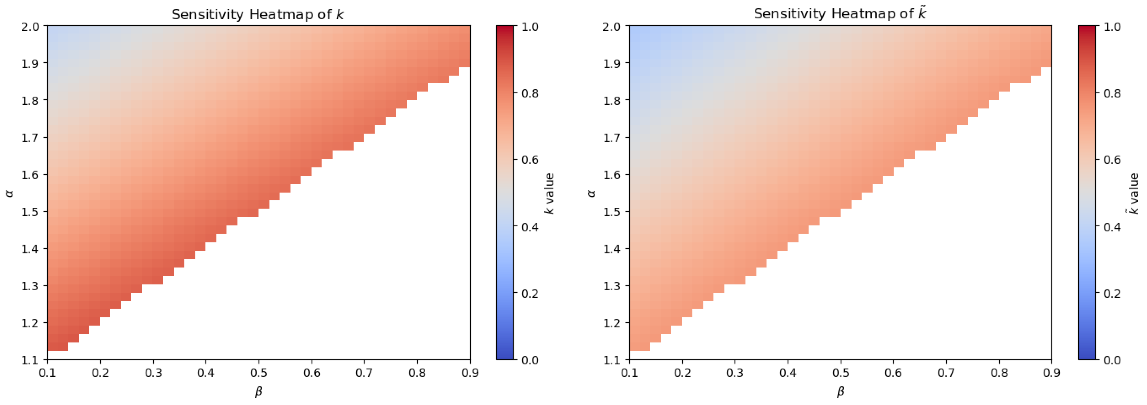
The heatmaps illustrated in Figure 8 represent the sensitivity of k and k ˜ over ( α , β ) . Lighter tones indicate smaller values and hence stronger contractions. For fixed β , both quantities decrease with increasing α and for fixed α , they increase with β . These trends confirm that larger α values relative to β improve the stability within the admissible region.

5. Memory-Dependent Learning and Behavioral Adaptation in Animals: An Application

This section applies the fractional models (4) and (5) to a learning process with memory. The state x ( t ) represents proficiency, and S ( t ) is an external stimulus. We consider
D t 1.03 x ( t ) + 1 12.25 D t 0.01 x ( t ) + 0.001 x ( t ) = S ( t ) , t [ 0 , 10 ] ,
with initial data
x ( 0 ) = 0.2 , x ( 0 ) = 0.1 .
The stimulus is a bounded Gaussian pulse train:
S ( t ) = A k = 1 N exp ( t t k ) 2 2 σ 2 , t [ 0 , 10 ] .
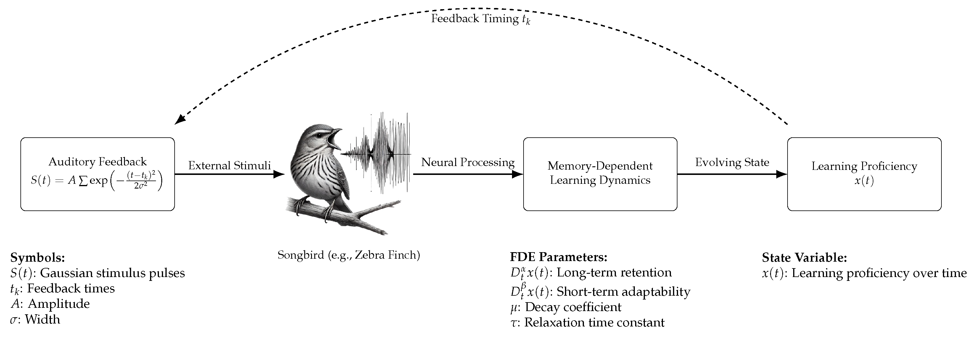
The orders α = 1.03 and β = 0.01 encode persistent memory and rapid responsiveness and satisfy α β = 1.02 > 1 . The parameters are μ = 0.001 , τ = 12.25 , t 0 = 0 , T = 10 . The term D t α x accounts for long-range history, D t β x captures short-term adaptation, and μ x models slow forgetting. The setup matches the empirical features of animal learning: for instance, vocal acquisition in songbirds, where x ( t ) measures accuracy, and S ( t ) represents periodic auditory feedback (see Figure 9).
To certify well-posedness for the learning model, we use the constants from Theorems 3 and 4. For the parameters in Equation (18), we obtain k = 0.9456 < 1 and k ˜ = 0.9339 < 1 . Hence, Z is a strict contraction and the hypotheses of Krasnosel’skii hold. Existence and uniqueness follow without further conditions.
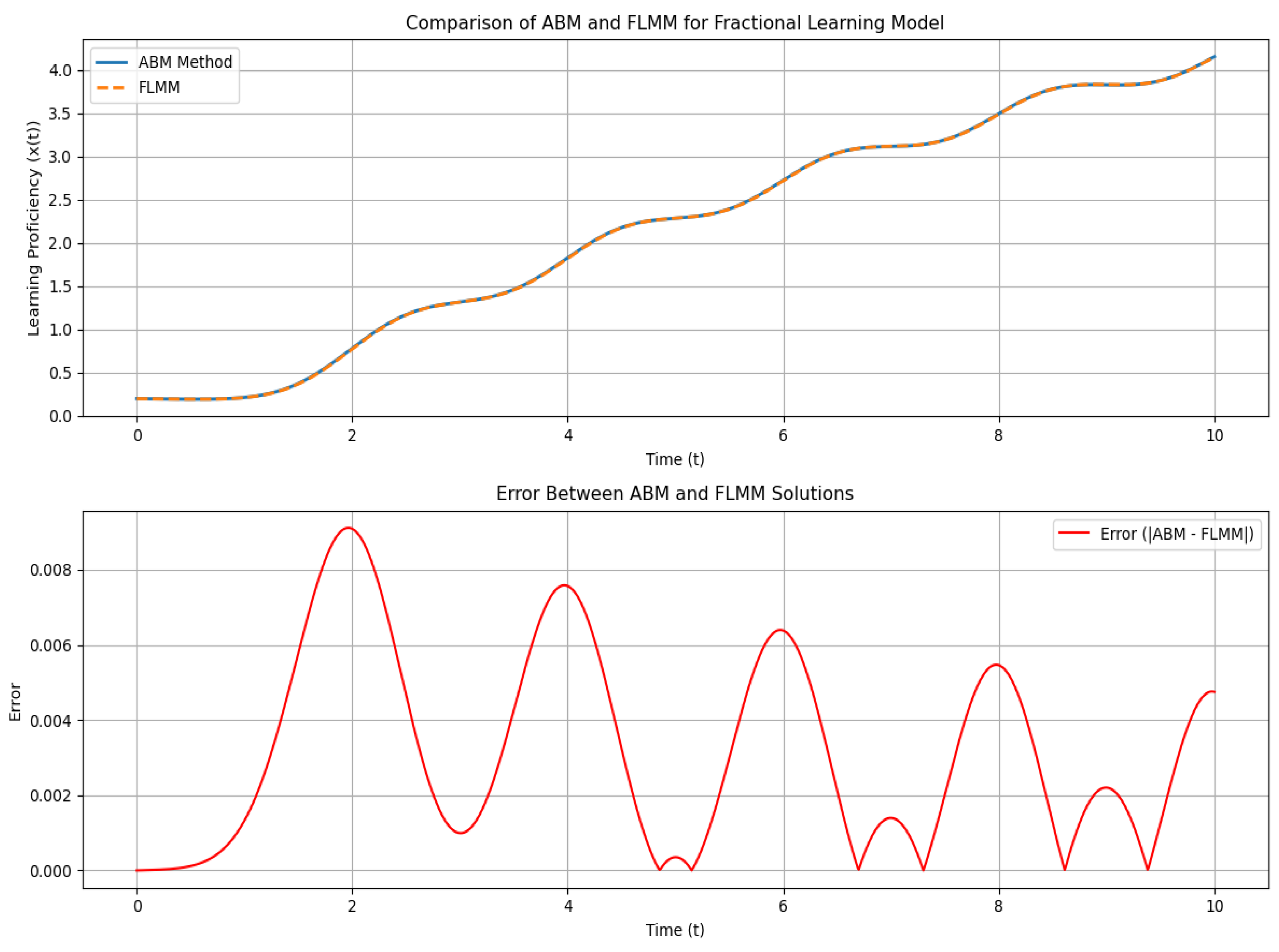
The numerical behavior is analyzed using two established schemes: the Adams–Bashforth–Moulton (ABM) predictor–corrector method [33] and the fractional linear multistep Method (FLMM) [34]. Pulse times are t k = { 1 , 3 , 5 , 7 , 9 } and t k = { 2 , 4 , 6 , 8 , 10 } with A = 1 and σ = 0.5 . Figure 10 compares ABM and FLMM together with the absolute error. Both resolve the stimulus-driven oscillations and remain close, with a maximum discrepancy below 8 × 10 3 . Figure 11 reports an alternative configuration and yields the same level of agreement.
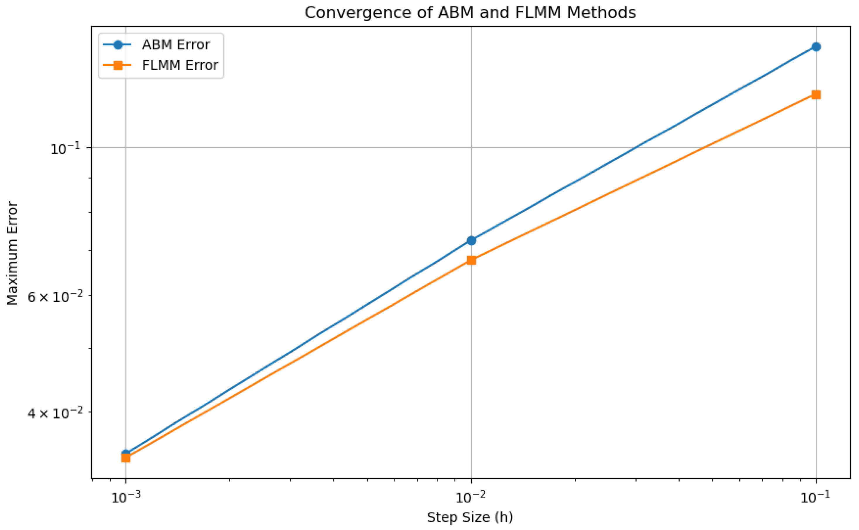
Figure 12 and Figure 13 display convergence for step sizes h { 10 1 , 10 2 , 10 3 } against a high-accuracy ABM reference at h = 10 4 . Both methods show first-order behavior. ABM is slightly sharper in Figure 13, while FLMM attains the smaller error in Figure 12, reflecting sensitivity to pulse timing.
The evolution of x ( t ) under varying ( α , β ) pairs is illustrated in Figure 14. The left panel considers a broad range within the stable region, while the right panel focuses on a narrow band where α β 1.1 . In the broader setting, solutions with larger α exhibit faster growth, reflecting stronger memory effects. Increased β values enhance sensitivity to the feedback pulses, inducing sharper local variations in x ( t ) . In the narrow-band simulations, the profiles remain closely aligned, suggesting that small perturbations in α and β yield quantitatively similar outcomes, provided that the system remains within the stable domain.
The numerical results for randomly selected pairs ( α , β ) with feedback events at t k = [ 1 , 3 , 5 , 7 , 9 ] are summarized in Table 1. Both ABM and FLM methods yield solutions in close agreement. The absolute error between them remains within the range 0.0078374 to 0.0085856 , while the RMSE values vary from 0.0035339 to 0.0054333 . These low error magnitudes confirm the reliability of both numerical schemes. The ABM method incurs a higher computational cost, with average runtimes near 0.013 seconds, compared to FLMM’s 0.005 seconds. The final learning proficiency x ( t ) increases monotonically with both α and β , indicating enhanced memory integration and adaptive responsiveness.
For the same random ( α , β ) pairs but with feedback events shifted to t k = [ 2 , 4 , 6 , 8 , 10 ] , the corresponding data are presented in Table 2. Learning proficiency values are consistently lower compared to the earlier case. The maximum error ranges from 0.0091103 to 0.0099865 , and RMSE values span 0.0040994 to 0.0063658 . These increases suggest a decline in learning efficiency when feedback is delayed. Runtimes remain stable across configurations. The shift in feedback timing leads to diminished cumulative effects of stimulus, highlighting the importance of reinforcement schedules in learning processes.
Table 3 contains results for non-randomly selected ( α , β ) values, retaining the original feedback times t k = [ 1 , 3 , 5 , 7 , 9 ] . The absolute error remains bounded within 0.0078689 to 0.0081061 , with RMSE between 0.0035803 and 0.0040715 . The numerical behavior mirrors the random parameter case, confirming the insensitivity of solution accuracy to specific ( α , β ) configurations within the stability region. The observed trend in x ( t ) supports the model’s robustness under controlled parameter variations. The ABM method again incurs higher runtimes, while FLMM achieves faster execution without loss of fidelity.
In Table 4, non-random parameter pairs are evaluated under the delayed feedback configuration t k = [ 2 , 4 , 6 , 8 , 10 ] . Learning proficiency levels decrease, with final values lower than those in earlier reinforcement scenarios. The error increases slightly, with maximum values ranging from 0.0091468 to 0.0094252 and RMSE between 0.004173 and 0.0048406 . This pattern reinforces the sensitivity of the learning model to the temporal distribution of external stimuli. Earlier feedback consistently results in higher proficiency gains.
Across our tests, learning outcomes depend on both the fractional orders and the timing of reinforcement: larger α sustains retention, larger β sharpens responsiveness, and earlier pulses yield greater proficiency. Between the two solvers, ABM is marginally more accurate at fixed steps, whereas FLMM attains comparable errors with lower cost. For fine accuracy targets or stiff transients, ABM is preferable, while FLMM is advantageous in large-scale or near-real-time runs. The dual-order formulation reflects long-term persistence together with fast adaptation and reproduces the observed sensitivity to feedback timing. The present example is illustrative rather than data-driven, and future work will fit ( α , β , μ , τ ) to experimental trajectories with recorded stimuli and compare single-order vs. dual-order kernels by out-of-sample errors, thereby providing quantitative validation.

6. Conclusions

In this work, we proposed a Caputo fractional model with two orders to describe learning dynamics with memory and external stimuli. Existence and uniqueness were obtained by fixed-point arguments. A parameter study quantified how the orders and coefficients shape solution trajectories and the stability region. We computed solutions with the Adams–Bashforth–Moulton (ABM) and fractional linear multistep method (FLMM) and compared accuracy and convergence. In a learning example with Gaussian pulses, earlier feedback produced larger gains. The term D t β x captures rapid alignment with recent input, while D t α x sustains proficiency in the absence of feedback. The framework provides a rigorous basis for systems with memory and suggests applications to biological learning and adaptive behavior. Future work will fit ( α , β , μ , τ ) to experimental trajectories with recorded stimuli and compare single-order versus dual-order kernels by out-of-sample errors. Extensions include nonlinear or state-dependent feedback, stochastic or subject-specific stimuli, and mixed-effect formulations to capture inter-individual variability.

Author Contributions

Conceptualization, A.T., J.-A.N.-S. and J.-J.T.; Methodology, A.T., W.A., A.M. and J.-J.T.; Validation, A.T., J.-A.N.-S. and A.M.; Formal analysis, J.-A.N.-S. and A.M.; Investigation, J.-A.N.-S., A.M. and J.-J.T.; Resources, W.A.; Data curation, W.A. and J.-J.T.; Writing—original draft, A.T.; Writing—review and editing: A.T., W.A. and J.-J.T.; Visualization, A.T. and W.A.; Supervision, A.M. and J.-J.T. All authors have read and agreed to the published version of the manuscript.

Funding

This research is supported by the University of Alicante, Spain; the Spanish Ministry of Science and Innovation; the Generalitat Valenciana, Spain; and the European Regional Development Fund (ERDF) through the following funding sources: At the national level, this work was funded by the following projects: TRIVIAL (PID2021-122263OB-C22) and CORTEX (PID2021-123956OB-I00), granted by MCIN/AEI/10.13039/501100011033 and, as appropriate, co-financed by “ERDF A way of making Europe”, the “European Union”, or the “European Union Next Generation EU/PRTR”. At the regional level, the Generalitat Valenciana (Conselleria d’Educació, Investigació, Cultura i Esport), Spain, provided funding for NL4DISMIS (CIPROM/2021/21).

Data Availability Statement

The original contributions presented in this study are included in this article. Further inquiries can be directed to the corresponding authors.

Conflicts of Interest

The authors declare no conflict of interest.

References

  1. Whitby, M.; Cardelli, L.; Kwiatkowska, M.; Laurenti, L.; Tribastone, M.; Tschaikowski, M. PID control of biochemical reaction networks. IEEE Trans. Autom. Control 2021, 67, 1023–1030. [Google Scholar] [CrossRef]
  2. Fröhlich, F.; Sorger, P.K. Fides: Reliable trust-region optimization for parameter estimation of ordinary differential equation models. PLoS Comput. Biol. 2022, 18, e1010322. [Google Scholar] [CrossRef] [PubMed]
  3. Linot, A.J.; Burby, J.W.; Tang, Q.; Balaprakash, P.; Graham, M.D.; Maulik, R. Stabilized neural ordinary differential equations for long-time forecasting of dynamical systems. J. Comput. Phys. 2023, 474, 111838. [Google Scholar] [CrossRef]
  4. Turab, A.; Sintunavarat, W. A unique solution of the iterative boundary value problem for a second-order differential equation approached by fixed point results. Alex. Eng. J. 2021, 60, 5797–5802. [Google Scholar] [CrossRef]
  5. He, L.; Valocchi, A.J.; Duarte, C.A. A transient global-local generalized FEM for parabolic and hyperbolic PDEs with multi-space/time scales. J. Comput. Phys. 2023, 488, 112179. [Google Scholar] [CrossRef]
  6. Zúñiga-Aguilar, C.J.; Gómez-Aguilar, J.F.; Romero-Ugalde, H.M.; Escobar-Jiménez, R.F.; Fernández-Anaya, G.; Alsaadi, F.E. Numerical solution of fractal-fractional Mittag–Leffler differential equations with variable-order using artificial neural networks. Eng. Comput. 2022, 38, 2669–2682. [Google Scholar] [CrossRef]
  7. Lakzian, H.; Gopal, D.; Sintunavarat, W. New fixed point results for mappings of contractive type with an application to nonlinear fractional differential equations. J. Fixed Point Theory Appl. 2016, 18, 251–266. [Google Scholar] [CrossRef]
  8. Rezaei, M.M.; Zohoor, H.; Haddadpour, H. Analytical solution for nonlinear dynamics of a rotating wind turbine blade under aerodynamic loading and yawed inflow effects. Thin-Walled Struct. 2025, 212, 113164. [Google Scholar] [CrossRef]
  9. Magazev, A.A.; Boldyreva, M.N. Schrödinger equations in electromagnetic fields: Symmetries and noncommutative integration. Symmetry 2021, 13, 1527. [Google Scholar] [CrossRef]
  10. Liu, Y.; Yang, Z.; Yu, Z.; Liu, Z.; Liu, D.; Lin, H.; Li, M.; Ma, S.; Avdeev, M.; Shi, S. Generative artificial intelligence and its applications in materials science: Current situation and future perspectives. J. Mater. 2023, 9, 798–816. [Google Scholar] [CrossRef]
  11. Hsu, S.B.; Chen, K.C. Ordinary Differential Equations with Applications; World Scientific: Singapore, 2022; Volume 23. [Google Scholar]
  12. Kai, Y.; Yin, Z. Linear structure and soliton molecules of Sharma-Tasso-Olver-Burgers equation. Phys. Lett. A 2022, 452, 128430. [Google Scholar] [CrossRef]
  13. Turab, A.; Montoyo, A.; Nescolarde-Selva, J.A. Stability and numerical solutions for second-order ordinary differential equations with application in mechanical systems. J. Appl. Math. Comput. 2024, 70, 5103–5128. [Google Scholar] [CrossRef]
  14. Brady, J.P.; Marmasse, C. Analysis of a simple avoidance situation: I. Experimental paradigm. Psychol. Rec. 1962, 12, 361. [Google Scholar] [CrossRef]
  15. Turab, A.; Montoyo, A.; Nescolarde-Selva, J.-A. Computational and analytical analysis of integral-differential equations for modeling avoidance learning behavior. J. Appl. Math. Comput. 2024, 70, 4423–4439. [Google Scholar] [CrossRef]
  16. Marmasse, C.; Brady, J.P. Analysis of a simple avoidance situation. II. A model. Bull. Math. Biophys. 1964, 26, 77–81. [Google Scholar] [CrossRef] [PubMed]
  17. Zhang, D.; Zhang, L.; Lan, T.; Wen, J.; Gao, L. A memory-dependent three-dimensional creep model for concrete. Case Stud. Constr. Mater. 2024, 20, e03289. [Google Scholar] [CrossRef]
  18. Ribeiro, H.V.; Tateishi, A.A.; Lenzi, E.K.; Magin, R.L.; Perc, M. Interplay between particle trapping and heterogeneity in anomalous diffusion. Commun. Phys. 2023, 6, 244. [Google Scholar] [CrossRef]
  19. Maurizi, M.; Gao, C.; Berto, F. Predicting stress, strain and deformation fields in materials and structures with graph neural networks. Sci. Rep. 2022, 12, 21834. [Google Scholar] [CrossRef]
  20. Lenzi, M.K.; Lenzi, E.K.; Guilherme, L.M.S.; Evangelista, L.R.; Ribeiro, H.V. Transient anomalous diffusion in heterogeneous media with stochastic resetting. Phys. A Stat. Mech. Its Appl. 2022, 588, 126560. [Google Scholar] [CrossRef]
  21. Hattaf, K. On the stability and numerical scheme of fractional differential equations with application to biology. Computation 2022, 10, 97. [Google Scholar] [CrossRef]
  22. Jajarmi, A.; Baleanu, D.; Sajjadi, S.S.; Nieto, J.J. Analysis and some applications of a regularized Ψ–Hilfer fractional derivative. J. Comput. Appl. Math. 2022, 415, 114476. [Google Scholar] [CrossRef]
  23. Özköse, F.; Yavuz, M.; Şenel, M.T.; Habbireeh, R. Fractional order modelling of omicron SARS-CoV-2 variant containing heart attack effect using real data from the United Kingdom. Chaos Solitons Fractals 2022, 157, 111954. [Google Scholar] [CrossRef] [PubMed]
  24. Sintunavarat, W.; Turab, A. A unified fixed point approach to study the existence of solutions for a class of fractional boundary value problems arising in a chemical graph theory. PLoS ONE 2022, 17, e0270148. [Google Scholar] [CrossRef]
  25. Almeida, R. A Caputo fractional derivative of a function with respect to another function. Commun. Nonlinear Sci. Numer. Simul. 2017, 44, 460–481. [Google Scholar] [CrossRef]
  26. Banach, S. Sur les opérations dans les ensembles abstraits et leur application aux équations intégrales. Fundam. Math. 1922, 3, 133–181. [Google Scholar] [CrossRef]
  27. Burton, T.A. A fixed-point theorem of Krasnoselskii. Appl. Math. Lett. 1998, 11, 85–88. [Google Scholar] [CrossRef]
  28. Kawamura, K.; Koshimizu, H.; Miura, T. Norms on C 1 ([0, 1]) and their isometries. Acta Sci. Math. 2018, 84, 239–261. [Google Scholar] [CrossRef]
  29. Kilbas, A.A.; Srivastava, H.M.; Trujillo, J.J. Theory and Applications of Fractional Differential Equations; Elsevier: Amsterdam, The Netherlands, 2006; Volume 204. [Google Scholar]
  30. Zhu, T. Global attractivity for fractional differential equations of Riemann-Liouville type. Fract. Calc. Appl. Anal. 2023, 26, 2264–2280. [Google Scholar] [CrossRef]
  31. Vu, H.; Rassias, J.M.; Hoa, N.V. Hyers–Ulam stability for boundary value problem of fractional differential equations with κ-Caputo fractional derivative. Math. Methods Appl. Sci. 2023, 46, 438–460. [Google Scholar] [CrossRef]
  32. Wang, X.; Luo, D.; Zhu, Q. Ulam-Hyers stability of caputo type fuzzy fractional differential equations with time-delays. Chaos Solitons Fractals 2022, 156, 111822. [Google Scholar] [CrossRef]
  33. Rosenfeld, J.A.; Dixon, W.E. Convergence rate estimates for the kernelized predictor corrector method for fractional order initial value problems. Fract. Calc. Appl. Anal. 2021, 24, 1879–1898. [Google Scholar] [CrossRef]
  34. Karaman, B. The global stability investigation of the mathematical design of a fractional-order HBV infection. J. Appl. Math. Comput. 2022, 68, 4759–4775. [Google Scholar] [CrossRef] [PubMed]
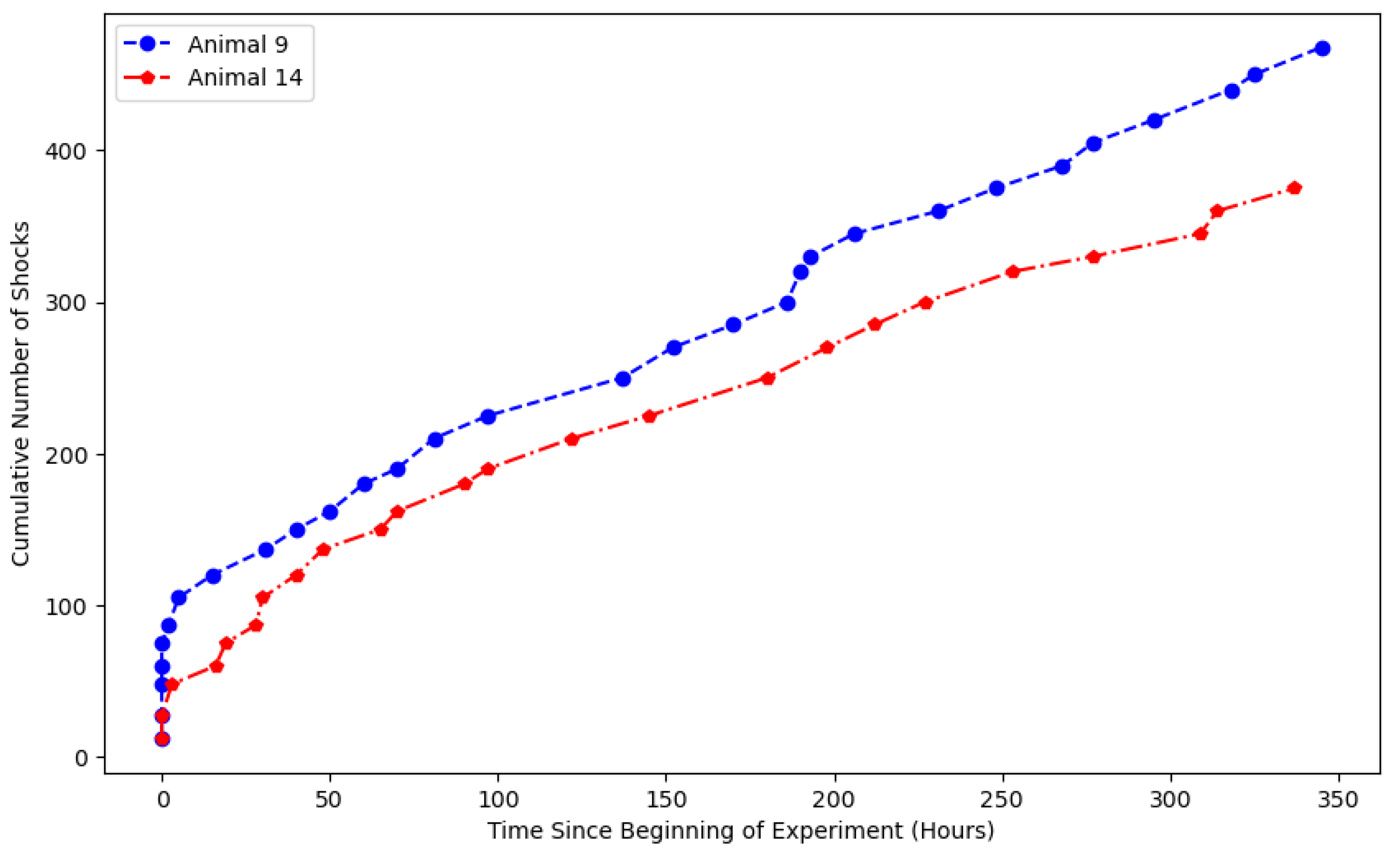
Figure 1. Experimental data from test animals.
Fractalfract 09 00664 g001
Figure 2. Data from control group.
Fractalfract 09 00664 g002
Figure 3. Picard iteration and its convergence.
Fractalfract 09 00664 g003
Figure 4. Stability region for FDE.
Fractalfract 09 00664 g004
Figure 5. Sensitivity of solution to α (fixed β = 0.9 ).
Fractalfract 09 00664 g005
Figure 6. Sensitivity of solution to β with fixed α .
Fractalfract 09 00664 g006
Figure 7. Effect of μ and τ on solution behavior.
Fractalfract 09 00664 g007
Figure 8. Sensitivity heatmap of k and k ˜ .
Fractalfract 09 00664 g008
Figure 9. Overview of the songbird vocal learning model. The stimulus S ( t ) induces memory-driven responses through Caputo derivatives D t α and D t β , yielding the learning proficiency x ( t ) .
Fractalfract 09 00664 g009
Figure 10. Comparison of ABM and FLMM with error analysis for t k = [ 1 , 3 , 5 , 7 , 9 ] .
Fractalfract 09 00664 g010
Figure 11. Comparison of ABM and FLMM with error analysis for t k = [ 2 , 4 , 6 , 8 , 10 ] .
Fractalfract 09 00664 g011
Figure 12. Convergence for t k = [ 1 , 3 , 5 , 7 , 9 ] .
Fractalfract 09 00664 g012
Figure 13. Convergence for t k = [ 2 , 4 , 6 , 8 , 10 ] .
Fractalfract 09 00664 g013
Figure 14. Solution of the fractional learning model with Gaussian pulse train stimulus.
Fractalfract 09 00664 g014
Table 1. Random α and β values with t k = [ 1 , 3 , 5 , 7 , 9 ] .
( α , β ) ABM SolutionFLMM SolutionMax ErrorRMSEABM Runtime (s)FLMM Runtime (s)
(1.02, 0.01)2.57512192.57321360.00783740.00353390.0261540.0068009
(1.10, 0.07)2.75768852.75510440.00800980.00384410.0127480.0054479
(1.23, 0.19)3.00608393.00248210.00825940.00449780.013720.005466
(1.35, 0.31)3.14435613.14015660.00841490.00496330.01265530.0052679
(1.47, 0.44)3.22195513.2174260.00851160.00524060.01259110.0052991
(1.55, 0.51)3.24568563.24106210.00854310.00532280.01288490.0054393
(1.67, 0.64)3.27113513.26642170.00857570.00540270.01264720.0052738
(1.78, 0.75)3.28187583.27713530.00858560.00542790.01257110.0053248
(1.89, 0.87)3.28788963.28314450.00858480.00543330.01460720.00545
(2.00, 0.98)3.29067743.28593940.00857750.00542790.0133610.005218
Table 2. Random α and β values with t k = [ 2 , 4 , 6 , 8 , 10 ] .
( α , β ) ABM SolutionFLMM SolutionMax ErrorRMSEABM Runtime (s)FLMM Runtime (s)
(1.02, 0.01)2.16918242.16633260.00911030.00409940.01907210.0071342
(1.10, 0.07)2.31005242.30653170.00931270.00454930.01235080.0051861
(1.23, 0.19)2.50139482.4968910.0096050.00534430.01228120.0052679
(1.35, 0.31)2.60818812.6031160.00978610.00586010.01232890.0051851
(1.47, 0.44)2.66850792.66312360.00989810.00615810.01262690.0051892
(1.55, 0.51)2.68708382.68160980.00993470.00624590.01222210.0052018
(1.67, 0.64)2.70714422.70158490.0099730.00633150.01273820.0052538
(1.78, 0.75)2.71569042.71010530.00998560.00635910.01252580.0052421
(1.89, 0.87)2.72051792.71492870.00998650.00636580.01263690.0057559
(2.00, 0.98)2.72277542.71719350.00998010.0063610.01314810.005378
Table 3. Non-random α and β values with t k = [ 1 , 3 , 5 , 7 , 9 ] .
( α , β ) ABM SolutionFLMM SolutionMax ErrorRMSEABM Runtime (s)FLMM Runtime (s)
(1.04, 0.02)2.60867142.60664410.00786890.00358030.02658770.0055413
(1.06, 0.03)2.64093992.63879590.00789920.00362940.012480.0052299
(1.08, 0.04)2.67195012.66969180.00792850.00368060.01234670.0052569
(1.12, 0.05)2.70172672.69935690.00795660.00373380.01238180.005203
(1.14, 0.06)2.73029672.72781820.00798370.00378840.01309990.0055909
(1.16, 0.07)2.75768852.75510440.00800980.00384410.01267980.0053079
(1.18, 0.08)2.78393222.78124540.00803510.00390060.01264190.0052891
(1.20, 0.09)2.80905872.80627250.00805970.00395750.01271320.0053508
(1.22, 0.10)2.83309992.83021760.00808340.00401460.01318980.0064509
(1.24, 0.11)2.85608862.85311330.00810610.00407150.01334930.0055439
Table 4. Non-random α and β values with t k = [ 2 , 4 , 6 , 8 , 10 ] .
( α , β ) ABM SolutionFLMM SolutionMax ErrorRMSEABM Runtime (s)FLMM Runtime (s)
(1.04, 0.02)2.19510162.19213220.00914680.0041730.02790310.008374
(1.06, 0.03)2.22001582.21692990.00918250.00424770.01236890.005197
(1.08, 0.04)2.24394562.2407460.00921690.00432310.0123580.0052168
(1.12, 0.05)2.26691262.26360280.009250.00439870.01230220.005199
(1.14, 0.06)2.28894022.28552330.00928190.00447420.01292320.0053151
(1.16, 0.07)2.31005242.30653170.00931270.00454930.01269670.00528
(1.18, 0.08)2.3302742.3266530.00934230.00462370.01263620.0052989
(1.20, 0.09)2.34963072.34591270.00937070.00469730.0126290.0052691
(1.22, 0.10)2.36814842.36433690.00939840.00476960.01267580.0052612
(1.24, 0.11)2.38585352.38195180.00942520.00484060.0127020.0053277
Disclaimer/Publisher’s Note: The statements, opinions and data contained in all publications are solely those of the individual author(s) and contributor(s) and not of MDPI and/or the editor(s). MDPI and/or the editor(s) disclaim responsibility for any injury to people or property resulting from any ideas, methods, instructions or products referred to in the content.