Abstract
Autonomous robotic navigation is essential in modern systems for revolutionising various industries that operate in both static and dynamic environments. To achieve this autonomous navigation, various conventional techniques that handle environment mapping, path planning, and motion control as individual modules often face challenges in addressing the complexities of autonomous navigation. Therefore, this paper presents an integrated technique that combines three essential components, such as environment mapping, path planning, and motion control, to enhance autonomous navigation performance. The first component, i.e., the mapping, utilises both binary and probabilistic occupancy maps to represent the environment. The second component is path planning, which incorporates various graph- and sampling-based algorithms such as PRM, A*, Hybrid A*, RRT, RRT*, and BiRRT, which are evaluated in terms of path length, computational time, and safety margin on various maps. The final component, i.e., motion control, utilises both conventional and advanced controller strategies such as PID, FOPID, SFC, and MPC, for better sinusoidal trajectory tracking. The four case studies for path planning and one case study on trajectory tracking on various occupancy maps demonstrated that the A* algorithm and MPC outperformed all the compared techniques in terms of optimal path length, computational time, safety margin, and trajectory tracking error. Thus, the proposed integrated approach reveals that the interplay between mapping fidelity, planning efficiency, and control robustness is vital for reliable autonomous navigation.
1. Introduction
Autonomous robotic navigation has emerged as one of the essential elements in modern systems for revolutionising various industries [1,2]. In multiple industries, for autonomous robotic navigation in static and dynamic environments, the robot’s ability to interpret the environment using occupancy maps [3,4], plan an optimal path using path planning techniques [5,6,7,8], and execute precise movements using control strategies is critical [9,10]. Thus, the need for an integrated framework utilising three fundamental components, including environment representation via occupancy maps, sampling-driven path planning, and motion control, is inevitable for enhancing performance during robotic autonomous navigation. In the literature, each of these components has been widely explored individually, and several studies also present comprehensive navigation frameworks. However, most emphasise particular aspects more strongly. For instance, the mapping algorithms have been evaluated on their fidelity [4]. On the other hand, path planning algorithms have been assessed based on their path efficiency, and motion control techniques have been evaluated based on their tracking performance [5,10]. However, for real-time robotic navigation, all these components are interconnected. An inaccurate mapping will affect the efficiency of path planning. The suboptimal path from these techniques may fail to achieve proper control action, hindering accurate follow of the optimal path.
Mapping and localisation are the first and crucial pillars for this integrated framework of autonomous navigation. Recently, in [11], a probabilistic 3D occupancy mapping framework known as OctoMap, which balances map fidelity with memory and runtime efficiency, was introduced. Each octree of the OctoMap stores the occupancy probability that supports large-scale mapping on embedded hardware. The geometry-aware 3D point cloud learning enables precise cutting-point detection in unstructured environments, supporting robust LiDAR-based navigation [12]. Similarly, the RTAB framework for large-scale SLAM, which utilises a memory-management strategy, has been proposed [13]. This type of framework has been widely adopted in ROS with inputs from LiDAR. The authors of [14,15] have introduced ORB-SLAM2 and ORB-SLAM3, respectively, which handle monocular, stereo, RGB-D, and multi-camera inputs and present an atlas of sub-maps with automatic place-recognition-based merging. However, the framework’s dependence on salient corners and challenges in textureless environments is notable. The KinectFusion framework for real-time dense surface mapping and online planning has been introduced [16]. This method fuses depth frames into a volumetric grid and simultaneously tracks using the camera.
The second pillar in autonomous robotic navigation is the use of path planning algorithms for finding an optimal path on environmental maps [17,18,19]. Dijkstra’s algorithm is the most widely used canonical single-source shortest path method for graphs with non-negative edge weights [20]. However, the major limitation of the technique is its computational cost on large maps. The A* path planning technique outperforms Dijkstra’s algorithm, which optimally searches towards the goal node with a heuristic cost function [21]. The algorithm is a standard technique for global path planning. However, the performance can degrade when heuristics are weak. The D* (or Dynamic A*) algorithm is an incremental replanning technique designed for dynamic environments that optimally replans from the start node when a new obstacle is detected [22]. However, implementing this method for continuous robot dynamics is a complex task.
Another variant of D* is the D* Lite algorithm, which plans the path by maintaining vertex keys [23]. This algorithm adapts to newly discovered obstacles in real-time. The ARA* algorithm introduces an inflation factor to the heuristic cost function [24]. The ARA* provides a suboptimal path at every iteration, making it feasible for all real-time systems. The Hybrid A* algorithm is an extension of the traditional A*, which searches in a 2D grid space, while Hybrid A* searches in a 3D continuous kinematic state space defined by the vehicle’s position and orientation . This orientation in Hybrid A* helps in producing smooth and feasible paths that a real vehicle can follow [5,6,7]. The PRM algorithm, on the other hand, samples the configuration space and connects samples with a local planner, and performs graph search to find a collision-free route [25,26,27]. The significant limitations of this technique include the upfront cost of constructing the roadmap and decreased efficiency due to frequent environmental changes.
The RRT algorithm is another path planning algorithm that rapidly expands in high-dimensional spaces to find a feasible path [28,29,30]. It achieves this by randomly sampling points in the free search space and connecting them to the nearest point in the existing tree, if feasible. The RRT* algorithm is an optimized variant of the traditional RRT algorithm, which improves the path over time by incorporating a rewiring step, which reduces the path length and achieves a smoother path [31]. The BiRRT algorithm is an extended version of the traditional RRT, where two trees grow simultaneously from the start and goal, unlike the RRT algorithm, which uses only one tree from the starting node [29]. Thus, by growing trees from both ends, the search space is explored more efficiently, making it suitable for high-dimensional spaces where direct single-tree exploration is slow. The BIT algorithm combines sampling, heuristic graph search, and optimization at every iteration. The BIT* is a variant of BIT that works on graph-like edge evaluations with tree rewiring [32].
The third and final pillar in autonomous robotic navigation is the use of motion control techniques for following the optimal path by controlling the robot’s drive components, such as motors and actuators. The PID controller is the most widely used to achieve this objective. An extension to PID, which is a kinematic fuzzy logic–based PID controller for following circular and point-to-point trajectories, has been introduced [33]. The controllers help to balance responsiveness and overshoot when curvature and speed vary along the path. However, the controller still oscillates near the sharp corners. Similarly, an intelligent PID with PD in the feedforward direction is proposed to achieve the robust trajectory tracking performance under disturbances and model uncertainty [34]. The authors of [35] have proposed the FOPID controller, and the authors of [36] have proposed the hybrid sliding mode with FOPID controllers for trajectory-tracking and maintaining stability. The two additional degrees of freedom in FOPID, namely, integral and derivative orders, facilitate achieving more robust performance. On the other hand, various researchers also proposed different control strategies for trajectory tracking. For instance, Wang et al. proposed a state feedback controller for achieving better real-time performance and robustness to speed and curvature changes [37]. Similarly, Villalba-Aguilera et al. implemented an MPC controller for tracking with online obstacle-aware shaping [38].
From the above literature, it is worth highlighting that conventional techniques, which handle environment mapping, path planning, and motion control as individual modules, often face challenges in addressing the complexities of autonomous navigation. This creates a clear motivation for developing an integrated framework that can manage these interdependent tasks of mapping, path planning, and motion control, thereby improving reliability and adaptability in real-world scenarios. Thus, this research proposes an integrated framework that combines all these components to achieve better autonomous navigation. The key contributions of this research are as follows: First, environmental representation through the use of multiple occupancy mapping techniques. Second, a comprehensive analysis of path planning algorithms, including PRM, A*, Hybrid A*, RRT, RRT*, and BiRRT. Third, an investigation of multiple motion control strategies, including PID, FOPID, SFC, and MPC, is conducted to assess their effectiveness during trajectory tracking.
The remaining sections of the paper are organised as follows: Section 2 presents the representation of the environment using occupancy-based maps such as binary and probabilistic mapping. Section 3 presents various path planning algorithms such as PRM, A*, and Hybrid A* algorithms, and the RRT family, which includes RRT, RRT*, and BiRRT for finding optimal paths on the occupancy maps. Section 4 presents motion control techniques, including PID, fractional-order PID, state feedback controller, and model predictive controller, for the robot to move along the desired path and achieve the desired speed at each moment. Section 5 presents the performance of various path planning algorithms on different occupancy maps and compares them in terms of path length, computational time, and safety margin. This section also presents the performance compression of various motion control techniques on following a sinusoidal path and compares them in terms of different performance metrics. Section 6 concludes the paper.
2. Environment Representation Using Occupancy-Based Mapping
Representing the environment is the first step in autonomous robotic navigation, which helps determine where a robot can and cannot go, as well as its ability to move safely and efficiently within the environment [39,40]. The environmental map will abstract the physical world into computable forms for better representation. The occupancy map is one such type of approach that represents the robot’s environment by dividing it into a grid of cells. As given in Table 1, the grid can be either 2D or 3D, with cells representing whether they are occupied by an obstacle or free.

Table 1.
Key characteristics and types of occupancy maps.
As described in Table 1, there are mainly two types of occupancy maps, which are the binary occupancy map and the probabilistic occupancy map. In a binary occupancy map, as the name suggests, each cell is assigned a binary value of either 1 or 0, indicating whether it is occupied or free, respectively. Similarly, the probabilistic occupancy map assigns a value to each cell, ranging from 0 to 1, that represents the occupancy status. A detailed description of both maps will be provided in the subsequent sections.
2.1. Binary Occupancy Maps
As mentioned earlier, a binary occupancy map represents the environment as a grid-based structure, which is typically a two-dimensional array. In which each cell is represented as either occupied (1) or free (0). The binary occupancy maps are often created using various techniques. The first and simplest method is manual creation, in which a plan is made by an operator utilising known environmental characteristics. This is especially helpful in simulated or controlled settings where the precise placement of obstacles is known in advance. An example of a manually defined binary occupancy map is shown in Figure 1a.
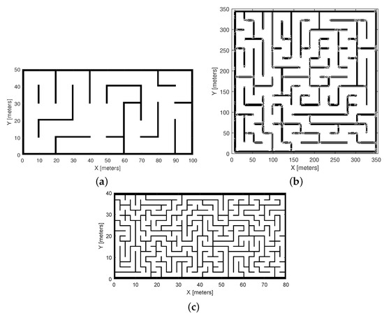
Figure 1.
Binary occupancy maps created: (a) manually defined to represent controlled environments, (b) derived from an image, and (c) randomly generated to emulate uncertain obstacle distributions.
Secondly, using thresholding algorithms to transform 2D photos into occupancy grids is a more dynamic and automated approach. In these situations, RGB or grayscale data are examined and converted to binary values using a cutoff point that separates the light (free) from the dark (occupied) areas (see Figure 1b). Finally, the creation of random binary maps is another popular technique that is useful for evaluating path planning algorithms in various uncertain situations, as shown in Figure 1c. Figure 1a illustrates a controlled environment with predetermined obstacles, whereas Figure 1c highlights uncertain scenarios where obstacles are randomly distributed, emulating unpredictable real-world conditions for robustness testing. It is worth highlighting that despite their ease of use and computational effectiveness, binary occupancy maps are not very effective at handling real-world complexity, including sensor noise, dynamic impediments, and partial observability.
2.2. Probabilistic Occupancy Maps
Similarly, the probabilistic occupancy map represents the environment as a discrete grid of cells, with cell values of approximately 1 indicating a high probability of occupancy or the presence of an obstacle, and values of approximately 0 indicating a high confidence level that the cell is free or empty space. The intermediate values, i.e., between 0 and 1, represent uncertain or partially observed regions. This enables the path planner to avoid potentially hazardous areas without relying on strict thresholds, select safer, lower-risk routes, and reason under uncertainty.
These maps are often created using sensor fusion methods that integrate data across time. LiDAR-based SLAM is one of the most popular methods for creating this type of probabilistic occupancy map, as it enables real-time updates to both the map and the robot’s current position. An example of such a probabilistic occupancy map created from LiDAR scans and poses is shown in Figure 2.
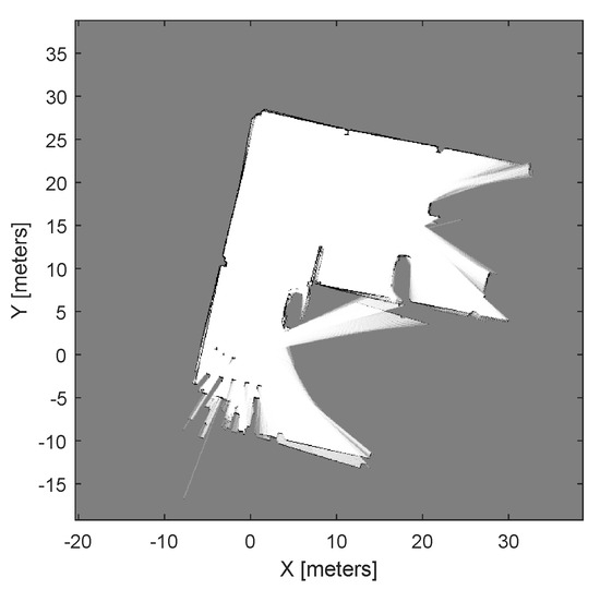
Figure 2.
Probabilistic occupancy map created from LiDAR scans and poses.
3. Sampling-Driven Path Planning Algorithms
After defining the occupancy map as explained in Section 2, the next essential part of autonomous robotic navigation is path planning. The path planning algorithms help the robot find the optimal path from the starting point to the destination point, avoiding all obstacles. The robot’s navigation capabilities mainly depend on the efficiency and robustness of the path planning algorithm employed.
Path planning algorithms can be broadly categorised into three main approaches: graph-based, sampling-based, and hybrid approaches. The graph-based algorithms will discretise the space into a grid or graph for finding the optimal path. However, the sampling-based techniques generate explicit graphs that are more suitable for continuous or high-dimensional domains. The hybrid approaches integrate motion feasibility and system dynamics into the design process.
As shown in Figure 3, the PRM, A*, and Hybrid A* algorithms and the RRT family, which includes RRT, RRT*, and BiRRT, are among the most well-known path planning techniques in autonomous robot navigation. The PRM builds a graph of collision-free configurations using random sampling and connects them to form a roadmap for path planning in static environments [25,26,27]. Moreover, the A* algorithm uses heuristics to find the shortest path on a grid. At the same time, the Hybrid A* algorithm extends it with continuous motion and vehicle kinematics to produce smoother, feasible paths [5,6,7]. The RRT algorithm explores the space rapidly by growing random trees. RRT* improves path optimality over time, and BiRRT grows trees from both start and goal for faster convergence [28,29,30]. These methods differ not only in their search strategy but also in their underlying representation: PRM relies on roadmaps, A* and Hybrid A* on grids/graphs, and RRT variants on random tree structures. A detailed description of these path planning techniques will be presented in the subsequent sections.
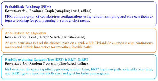
Figure 3.
Overview of key path planning algorithms for autonomous navigation, categorised by their representation type. PRM represents the environment as a roadmap graph, and A* and Hybrid A* utilise grid or graph search with heuristics. In contrast, RRT variants rely on random tree expansion.
3.1. Probabilistic Roadmap (PRM)
As mentioned earlier, the PRM is a sampling-based path planning technique that creates a roadmap, a network of paths that avoid collisions, by randomly selecting viable configurations from the environment and connecting them using basic local planners [25,26,27]. The flowchart of the PRM algorithm illustrating its implementation phases is shown in Figure 4. As shown in the figure, the algorithm consists of two distinct phases: the construction phase and the query phase.
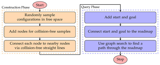
Figure 4.
Flowchart of the PRM algorithm illustrating its construction and query phases.
During the construction phase, first, random samples will be drawn from the robot’s configuration space. Then, each sample will be checked for collision. All free samples that are collision-free will be retained as nodes. Secondly, the algorithm attempts to connect these nodes to the neighbouring nodes using a basic local planner. The connections will only be added if there is an available, direct, and collision-free path between them. Finally, this process repeats to build a roadmap that represents the feasible connectivity in the environment. Further, during the query phase, the start and goal will be connected to the existing roadmap using the same collision-free criteria. Then, the standard graph search algorithms will be applied to the map to find the feasible path from the start to the goal.
3.2. A* and Hybrid A* Algorithms
Similarly, the A* algorithm is a graph-based path planning technique that finds the optimal path from the starting and the destination nodes in a weighted graph [5,6,7]. Using the following formula, the A* algorithm combines the actual cost from the start node to the given node n and the heuristic estimated cost to reach the destination or goal node from the node n.
The four most commonly used heuristic cost functions by the A* algorithm are Manhattan, Euclidean, Euclidean Squared, and Chebyshev, which are computed as follows:
The implementation flowchart of the A* algorithm is shown in Figure 5. As illustrated in the figure, the algorithm comprises four phases. Firstly, the initialisation phase involves creating two lists. The open list collects nodes that are candidates for exploration, and the closed list contains nodes that have already been examined. The start node is added to the open list, and the cost from the starting point is set to zero. The total estimated cost for reaching the goal from the start node is computed using the cost function in (1). The second phase is the exploration phase, in which the algorithm repeatedly examines the node n in the Open list that has the lowest estimated total cost value . During this phase, the A* algorithm efficiently narrows its search towards the goal by always choosing the most promising successor node. During this process, if the currently selected node happens to be the goal node, then the algorithm stops and proceeds to reconstruct the path; else, it moves on to further exploration and the successor generation phase.
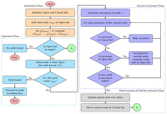
Figure 5.
Flowchart of the A* algorithm illustrating its phases.
The next phase is the successor generation phase, during which, if the goal node has not yet been reached, the algorithm generates all possible successors from the current node. Each successor is checked for validity by comparing it with both the open and closed lists. For all the valid successors, the associated costs such as , , and are calculated using the heuristic cost functions given in (2) to (5). The final phase is the node expansion and path reconstruction phase. In this phase, the algorithm progresses by moving the current node n from the open to the closed lists. For each valid successor, the algorithm determines whether it should be added to the open list, updated with better cost or parent information, or ignored if it has already been processed under better conditions. When the goal node is reached, the algorithm makes use of parent pointers that were stored during exploration to trace back from the goal to the start node . By following these parent relationships, it efficiently builds the sequence of steps that constitute the optimal path found. This ensures that the result is both minimal in cost and valid concerning the constraints and heuristics used in the search.
The Hybrid A* algorithm is an extension of the traditional A*, which searches in a 2D grid space, while Hybrid A* searches in a 3D continuous kinematic state space defined by the vehicle’s position and orientation . This orientation in Hybrid A* helps in producing smooth and feasible paths that a real vehicle can follow. The key features of this algorithm include path planning in a 3D continuous state space, encompassing orientation, as well as handling both forward and reverse motions. The algorithm further checks for collisions using state validators on occupancy maps and uses the cost function combining actual cost and heuristic, defined as follows:
where is the actual cost from the start node to the current node, and is the heuristic estimated cost to reach the goal node with orientation , which is computed as
where is the goal state, and is a weight factor.
3.3. Rapidly Exploring Random Tree (RRT)
The RRT algorithm is another path planning algorithm that rapidly expands in high-dimensional spaces to find a feasible path [28,29,30]. It achieves this by randomly sampling points in the free search space and connecting them to the nearest point in the existing tree, if feasible. This approach biases growth towards unexplored areas, enabling efficient coverage of large and complex environments. The RRT-based algorithm is divided into five phases, as illustrated in Figure 6. During the initialisation phase, the algorithm initialises the tree from the start or root node. Next, during the random sampling phase, the samples will be generated randomly from the free search space. Then, the algorithm identifies the node in the existing tree that is nearest to the random sample during the nearest node selection process. Then, during the extension phase, the tree attempts to extend from the nearest node towards the random sample, up to a specified step size. If the new position is obstacle-free, it becomes a new node with an edge connecting it to the nearest node. Otherwise, it will discard both the new node and the tree extension. Finally, during the termination phase, this process repeats until a node reaches sufficiently close to the goal or a maximum number of iterations is completed.
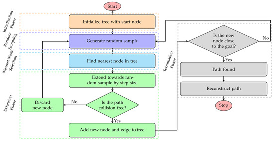
Figure 6.
Flowchart of the RRT algorithm illustrating its phases.
The RRT* algorithm is an optimized variant of the traditional RRT algorithm, which improves the path over time by incorporating a rewiring step, which reduces the path length and achieves a smoother path [31]. The flowchart of the RRT* algorithm, illustrating its phases including the rewiring step, is shown in Figure 7. As shown in the figure, during the initialisation phase, the algorithm initialises the tree with the starting node. During the sampling phase, the algorithm generates a random sample in the configuration space and selects the goal state directly to guide the search, a method known as goal-direct sampling. During the nearest node selection, the algorithm finds the nearest nodes in the existing tree to the sampled point. The extension and rewiring phase is the crucial phase in this algorithm. During this phase, the algorithm extends the tree in the same way as the RRT algorithm from the nearest node towards the sampled point. If the new edge is collision-free, then it will add the new node and the edge to the tree. If a collision occurs, the new node will be discarded. Further, the RRT* algorithm adds a rewiring step, which identifies the nearby nodes within the search radius. Then select the parent node for the new node that results in the lowest total cost. Further rewiring of nearby nodes occurs if connecting through the new node yields a shorter path. Finally, during the termination phase, the algorithm checks if the new node is within the goal region. Then, it will record the path and update the best shortest path. Finally, the algorithm reconstructs the optimal path from start to goal using the final tree structure.
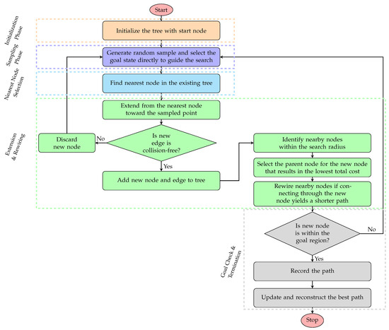
Figure 7.
Flowchart of the RRT* algorithm illustrating its phases.
The BiRRT is an extended version of the traditional RRT, where two trees grow simultaneously from the start and goal, unlike the RRT algorithm, which uses only one tree from the starting node [29]. Thus, by growing trees from both ends, the search space is explored more efficiently, making it suitable for high-dimensional spaces where direct single-tree exploration is slow. Similarly, the implementation flowchart of the BiRRT algorithm illustrating its six phases is shown in Figure 8. As illustrated in the figure, the algorithm proceeds through five phases. Firstly, during the initialisation phase, the algorithm initialises both trees, Tree A from the starting node and Tree B from the goal node. Similar to RRT*, during the sampling phase, the BiRRT algorithm also generates a random sample in the configuration space. It selects the goal state directly to guide the search, a method known as goal-direct sampling. During the expansion phase, both trees will find and expand towards the nearest node. For both trees, if the new edge is collision-free, then it will add the new node and the edge to the tree. If a collision occurs, the new node will be discarded. As both the trees expand simultaneously in this phase, the search space is explored more efficiently. The next phase is the connection and path reconstruction phase. During this phase, the algorithm checks if Tree B or the goal tree successfully connects to the new node in Tree A or the start tree, and then constructs the path. Otherwise, the algorithm proceeds to its final phase, known as the alternation or swapping phase. In this phase, the algorithm swaps the roles of both trees and continues from the samples phase by regenerating the random samples.
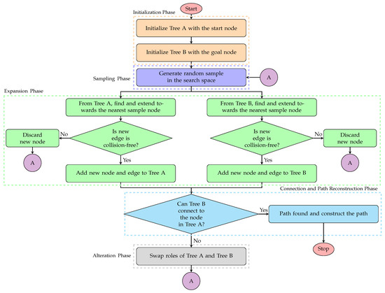
Figure 8.
Flowchart of the BiRRT algorithm illustrating its phases.
4. Advanced Motion Control Techniques
After obtaining the optimal path using the path planning techniques as explained in the previous section, the next essential part of autonomous robotic navigation is motion control. The motion control techniques will help the robot move along this path by controlling its drive components, such as motors and actuators, to achieve the desired speed at each moment. The path planning algorithms in Section 3 help decide where the robot should go in the occupancy maps defined in Section 2. The motion control techniques help determine how the robot, driven by DC motors, gets there. The motors in the robot require a precise control signal to achieve the target motion. To achieve this, this research employs four control strategies, including PID, fractional-order PID, state feedback control, and modern predictive controllers. These controllers help in accurately regulating speed and ensure the robot tracks the planned path reliably.
4.1. PID and Fractional-Order PID Controllers (FOPIDs)
The PID controller is one of the most commonly used feedback control systems, which maintains a desired output, namely the speed of the robot, by adjusting its inputs [41]. The controller combines three actions: the proportional part with gain to respond to present error, the integral part with gain to eliminate past error, and the derivative part with gain to anticipate future error. The controller equation in the time domain is defined as
where is the tracking error. Further, the transfer function of the PID controller in Laplace domain s is given as
From the above PID controllers time domain and transfer function, the FOPID controllers equations can be achieved by replacing the integral and derivative actions with fractional orders of and , respectively, [41,42,43], as
The block diagrams of PID and FOPID controllers for the speed control of the simplified vehicle model are shown in Figure 9a and Figure 9b, respectively.
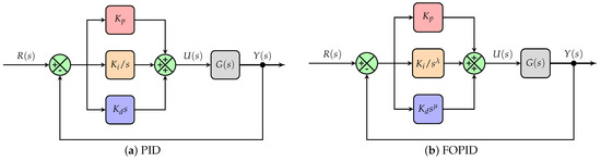
Figure 9.
Block diagrams of PID and FOPID controllers.
4.2. State Feedback Controller (SFC)
Unlike the PID controller that uses the transfer function model of the robot, the SFC uses state variables of the system to compute the control input using a constant gain matrix K defined as [44]
The block diagram of SFC controllers for the speed control of the simplified vehicle model defined in state-space form is shown in Figure 10. As shown in the figure, the system is represented in state-space as
where A, B, and C are the system, input, and output matrices. , , and are the state, input and output vectors.
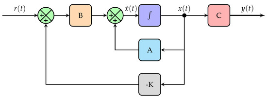
Figure 10.
Block diagrams of SFC controller.
4.3. Model Predictive Controller (MPC)
MPC is an advanced control strategy that uses a model to predict the future behaviour of a system and optimizes control actions over a finite prediction horizon p, subject to constraints [45]. Unlike the SFC, the MPC controller is designed for a system represented in discrete-time state-space form, as follows:
where A, B, and C are the system, input, and output matrices. , , and are the state, input, and output vectors at time step k.
The block diagram of the MPC controller is shown in Figure 11. As shown in the figure, the above discrete-time state-space model is used to predict the system’s future state and output over a prediction horizon p. At each step, the MPC controller computes the optimal sequence of control inputs by minimising the cost function J, defined as
where is the reference trajectory, Q and R are the tuned weighting matrices to find the future control inputs .
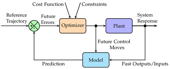
Figure 11.
Block diagrams of MPC controller.
5. Results and Discussions
5.1. Performance Analysis of Path Planning Algorithms
This section presents the performance analysis of path planning algorithms given in Section 3 on the occupancy maps created in Section 2.
5.1.1. Case 1: Manually Defined Map
In this case study, the performance of all path planning algorithms given in Section 3 is evaluated on a manually generated occupancy map given in Figure 1a. The detailed performance comparison of various path planning algorithms, highlighting both qualitative behaviours and quantitative path length, computation time, and safety margin (i.e., the average distance maintained from the planned path and the nearest obstacle) results on a manually defined occupancy map, is shown in Figure 12 and Table 2. As shown in the figure and the table, the PRM method has achieved a path length of 136.89 m by constructing a collision-free network of sampled nodes (see Figure 12a). However, the PRM’s path will heavily depend on node density and also require significant preprocessing for reliability. On the other hand, the A* algorithm with both Euclidean and Chebyshev cost functions has achieved a path length of 129.30 m, which is the shortest path among all the compared methods. This is because the algorithm’s efficient heuristics allow the algorithm to perform optimal search in direct and diagonal movements (see Figure 12b,c). Moreover, the A* algorithm with the Manhattan cost function has also achieved the shortest path of 129.30 m in length, but restricted movements to orthogonal steps and produces a more angular trajectory (see Figure 12d). The A* algorithm with Euclidean Squared cost function has produced a longer path of length 166.08 m due to the higher penalties on longer moves and altering the route geometry (see Figure 12e). The Hybrid A* algorithm, which incorporates vehicle kinematics to generate smooth and drivable curves, has achieved a slightly longer path length of 131.86 m compared to the traditional A* algorithm but achieved a feasible path (see Figure 12f).
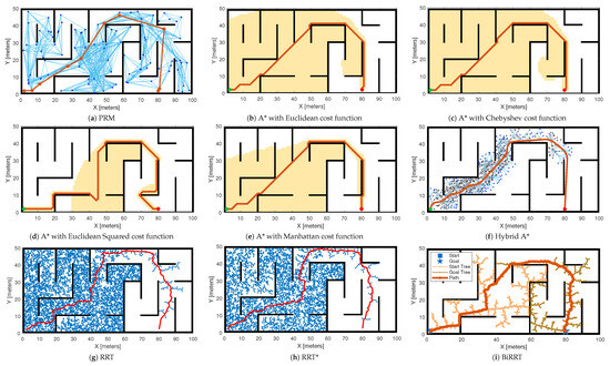
Figure 12.
Performance comparison of path planning algorithms on a manually defined occupancy map.
Table 2.
Numerical performance comparison of various path planning algorithms on different occupancy maps.
The conventional RRT quickly found a viable path with 169.82 m, but without optimal guarantees. The RRT* improved path smoothness and connectivity, but achieved a long 170.07 m path due to map constraints and sampling bias. The BiRRT achieved a 160.12 m path by simultaneously growing two trees from the start and goal, with faster convergence than the RRT algorithm. It is worth highlighting that all the sampling-based algorithms have produced longer paths due to their exploratory nature (see Figure 12g–i). Overall, the grid-based A* algorithm with Euclidean and Chebyshev metrics delivers the best optimal path, demonstrating superior path efficiency for this occupancy map.
The computational times shown in Table 2 indicate that the PRM technique completed in 0.082 s, whereas the A* algorithm with all four cost functions achieved the shortest times, ranging from around 0.006 to 0.008 s. In contrast, the Hybrid A* algorithm has a higher computational time of 0.325 s. On the other hand, the RRT family, including RRT, RRT*, and BiRRT, has the largest computational times, ranging from 3 to 5 s. This reflects the trade-off between exploration and efficiency. Further, the safety margins given in Table 2 show that the PRM maintained a moderate clearance, whereas the A* algorithm with all four cost functions achieved the paths with safety margins of 1.24 to 1.52 m. Moreover, the Hybrid A* algorithm provided a slightly better safety margin of 1.29 m, while RRT, RRT*, and BiRRT offered the highest safety margin up to 1.58 m. This indicates that the A* algorithm provides the shortest path in less computational time. At the same time, RRT techniques offer paths with the highest safety margins, albeit at the expense of longer paths and higher computational times.
5.1.2. Case 2: Map Created from Image
Similarly, in this case study, the performance of all path planning algorithms given in Section 3 is evaluated on an occupancy map generated from an image as presented in Figure 1b. Figure 13 presents the detailed performance evaluation of various path planning algorithms on a large, maze-like occupancy map generated from an image. Also, Table 2 presents the quantitative path length, computation time, and safety margin results for all the compared techniques. As shown in Figure 13a, the PRM technique has produced a feasible path with a length of 738.37 m by creating a dense network with 2000 node samples to capture narrow corridors and complex turns. On the other hand, among the grid-based techniques, as shown in Figure 13b,c, A* with Euclidean and Chebyshev cost functions has achieved the shortest path lengths of 735.46 m and 737.22 m, respectively. This is because the algorithm benefited from an optimal search that allows diagonal movements. The A* algorithm with the Manhattan function shown in Figure 13d has achieved a longer path of 756.17 m due to its restriction to orthogonal moves, which results in less direct routes in maze-like environments. Moreover, the A* algorithm with Euclidean Squared (see Figure 13e) has produced a significantly longer path of 860.98 m due to longer steps and additional detours. Hybrid A* has performed better among all the compared techniques and produced a shortest path of 726.05 m while maintaining kinematic feasibility, demonstrating its ability to generate smooth curves that reduce unnecessary detours (see Figure 13f).
Figure 13.
Performance comparison of path planning algorithms on an occupancy map created from an image.
Similar to Case 1, the sampling-based algorithms shown in Figure 13g–i have achieved longer paths due to their stochastic exploration. The RRT generated a longest path of 973.55 m due to its tendency to prioritise feasibility over optimality. The performance of RRT* has improved upon RRT by incremental path refinement and reducing the path length to 953.04 m. In comparison, the BiRRT achieved further improvement with a reduced path length of 922.11 m by simultaneously growing trees from the start and goal nodes. However, all RRT-based algorithms produced paths substantially longer than the grid-based techniques, indicating reduced efficiency in tightly constrained, corridor-dense maps. Overall, for this large and intricate map, Hybrid A* provided the most competitive balance between path efficiency and motion feasibility, outperforming all other compared techniques.
Similarly, the computational times in Table 2 highlight that the PRM technique required a significantly higher computational time of around 64.731 s, compared to the A* algorithm with all four cost functions, which had computation times ranging from 0.061 to 0.131 s. The Hybrid A* algorithm, however, showed a considerably larger computation time of 22.58 s due to its additional consideration of vehicle kinematics. In comparison, the RRT family (RRT, RRT*, and BiRRT) demonstrated moderate computational costs ranging between 5.884 and 7.198 s. Regarding safety margins, the PRM achieved a relatively high clearance of 3.50 m, while the A* variants delivered lower but consistent safety margins of around 0.51 m. The Hybrid A* algorithm achieved a safety margin of 3.28 m, showing a good trade-off between feasibility and clearance. On the other hand, the RRT, RRT*, and BiRRT algorithms produced the highest safety margins, ranging from 3.73 to 4.06 m, but at the expense of longer path lengths and higher computational requirements. Similar to Case 1, these results also indicate that while A* algorithms remain computationally efficient and deliver shorter paths, sampling-based RRT methods provide safer solutions but at a higher computational cost.
5.1.3. Case 3: Map Created from LiDAR Scans and Poses
Similarly, the performance of all path planning algorithms presented in Section 3 is evaluated on an occupancy map created from LiDAR scans and poses, as shown in Figure 2. Figure 14 presents a comparative assessment of various path planning algorithms applied to this probabilistic occupancy map, highlighting their exploration characteristics and the resulting paths. Table 2 also presents the quantitative path length, computation time and safety margin results for all the compared techniques for this map. The constructed path by the PRM technique in Figure 14a shows a graph of randomly sampled nodes connected by collision-free edges that produces a feasible path length of 38.39 m. As explained earlier, the technique’s performance depends solely on the sampling density.
Figure 14.
Performance comparison of path planning algorithms on an occupancy map created from LiDAR scans and poses.
The performance of the A* family of algorithms shown in Figure 14b–e demonstrates deterministic grid-based searches, with slight differences based on the cost functions. The A* with Euclidean heuristic produces a more direct route of path length 39.59 m. In comparison, A* with the Chebyshev function produced the same path length of 39.59 m using its efficient diagonal movements and potentially reducing path turns. Moreover, the A* with Euclidean-squared generated a longer path length of 40.58 m by moving more heavily and altering path geometry. In contrast, the A* with Manhattan function produced a path length of 39.83 m by restricting its motion to cardinal directions and creating more angular trajectories. On the other hand, Hybrid A*, shown in Figure 14f, produced a smooth path with a length of 40.29 m via drivable curves at the expense of higher computational demand.
Similar to cases 1 and 2, the sampling-based planners in this case also exhibit distinct trade-offs. The path by RRT shown in Figure 14f rapidly found the feasible solution with a path length of 55.36 m, though with less optimal and more irregular paths. The RRT* produced a shorter path, 43.10 m, than the RRT by incrementally rewiring its search tree for shorter, smoother routes, though at a higher computational cost. The BiRRT also outperformed the RRT by producing a feasible path of 49.05 m by growing two trees from the start and goal until they meet. Overall, the A* algorithm excels in generating a short and predictable path on a probabilistic occupancy map.
For Case 3, Table 2 shows that the PRM required 0.721 s of computation, which is higher than the A* algorithm variants, whose computational times ranged from 0.112 to 0.165 s. In contrast, the Hybrid A* algorithm had a significantly longer computational time of 20.766 s, due to the additional complexity of generating smooth kinematic paths. Interestingly, the RRT family was very efficient in this case, producing computational times ranging from 0.031 to 0.065 s, which is lower than both PRM and A*. Regarding safety margins, the PRM achieved a relatively low clearance of 0.18 m, while the A* variants achieved safety margins in the range of 1.02 to 1.06 m. Hybrid A* produced the highest margin of 1.59 m, showing an effective balance of feasibility and safety. Meanwhile, RRT, RRT*, and BiRRT offered higher safety margins, ranging from 1.27 to 3.11 m, indicating safer navigation, but often at the expense of longer paths. Unlike cases 1 and 2, this case demonstrates that RRT-based methods can achieve fast convergence and large safety margins, while A* remains more efficient in path optimality.
5.1.4. Case 4: Randomly Generated Map
Similarly, the performance of all path planning algorithms given in Section 3 is evaluated on a randomly generated complex occupancy map as presented in Figure 1c. Figure 15 and Table 2 present a comparative evaluation of all these path planning algorithms on a randomly generated complex occupancy map, highlighting both deterministic and sampling-based strategies and their respective adaptation to intricate environments. The PRM’s response, shown in Figure 15a, depicts a network of randomly distributed nodes and through collision-free connections, which achieved a feasible path of 480.72 m in length. However, as shown in the figure, the technique’s performance in this complex map is strongly dependent on higher sampling node density and connectivity. A lower sampling rate will result in a suboptimal path and exhibit excessive detours.
Figure 15.
Performance comparison of path planning algorithms on a randomly generated complex occupancy map.
The A* algorithm with its four cost function variants shown in Figure 15b–e demonstrates strong deterministic performance on grid-based representations of this on a randomly generated complex occupancy map. First, the A* with Euclidean cost function identifies the most direct route of 421.00 m that efficiently navigates the intricate corridors. Second, the A* with Chebyshev of 422.29 m further supports diagonal transitions, maintaining its optimality and smoothness in open regions. Thirdly, the A* with Euclidean Squared cost of 463.73 m has a slightly increased path length due to its quadratic weighting. Finally, the A* with Manhattan cost function limits movements to grid-aligned directions and produced more angular trajectories of 429.90 m path length. The Hybrid A*, which extended the traditional A* by including vehicle kinematic constraints, resulted in smooth, feasible trajectories of 700.82 m in length. Although the path length exceeds that of A*, the algorithm ensures that physical motion constraints are maintained.
It is worth highlighting that for this highly cluttered and randomly generated complex map, all the sampling-based planners, RRT, RRT*, and BiRRT, did not succeed in completing a collision-free path. This is because the intrinsic randomness and reliance on open passages often lead to failed paths with constrained connectivity and narrow corridors. Overall, the results illustrate that A* and Hybrid A* excel in finding efficient, predictable paths in this randomly generated complex map.
In Case 4, the results in Table 2 indicate that PRM required 64.40 s of computation, similar to Case 2, whereas the A* algorithm variants have the fastest computational times between 0.101 and 0.144 s. The Hybrid A* method was computationally expensive, requiring 136.39 s, reflecting the increased complexity in larger maps. In terms of safety margins, PRM achieved only 0.20 m, while all A* variants yielded zero clearance, indicating that their optimal paths cut very close to obstacles. Hybrid A* maintained a slightly better margin of 0.18 m, though still quite small. Similar to earlier cases, A* algorithms guarantee the optimal paths with low computation time, though at the expense of safety clearance.
5.2. Performance Analysis of Motion Control Techniques
In this section, the performance of all motion control techniques given in Section 4 is evaluated on the following vehicle longitudinal dynamics model. This section also represents the integration between path planning and motion control through the use of a sinusoidal reference trajectory under ideal conditions and in the presence of dynamic disturbances, to simulate real-world uncertainties. The nonlinear continuous-time vehicle model is given by
where
- —longitudinal position of the vehicle [m];
- —longitudinal velocity of the vehicle [m/s];
- —longitudinal acceleration of the vehicle [m/s2];
- m—mass of the vehicle [kg];
- —net tractive/braking force applied at the wheels [N];
- —air density [kg/m3];
- —aerodynamic drag coefficient;
- A—frontal cross-sectional area of the vehicle [m2];
- g—gravitational acceleration ( m/s2);
- —road slope angle [rad];
- —rolling resistance coefficient;
- —measured output, taken as the vehicle longitudinal velocity [m/s].
The coefficient values used in this work are kg/m3, , m2, and kg. The tuned parameters of PID and FOPID controllers using a trial-and-error approach for the control of a vehicle in (16) for following a sinusoidal path are , , , and . Similarly, during the design of SFC for obtaining K, the desired settling time and maximum overshoot are chosen as 2 and 0.05, respectively. On the other hand, the prediction and control horizons used during the design of MPC are 60 and 10, respectively. The performance comparison of all these motion control techniques, such as PID, FOPID, SFC, and MPC, for following a sinusoidal path defined by is shown in Figure 16.
Figure 16.
Performance comparison of various motion control techniques for following a sinusoidal path.
The numerical performance of these controllers is evaluated based on the tracking error , which is computed as follows:
where is the reference speed and is the actual speed. From the above error , the performance metrics used in this work, such as MAE, RMSE, and IAE, are computed as
where N is the number of samples and T is the total simulation time. The numerical performance comparison of these controllers in terms of MAE, RMSE, and IAE is given in Table 3.
Table 3.
Numerical performance comparison of motion control techniques on a sinusoidal path without and with dynamic disturbances.
From Figure 16 and Table 3, it is evident that the PID controller exhibits noticeable overshoot and steady-state deviations, with the highest tracking errors, MAE, RMSE, and IAE of 1.40, 2.26, and 140.19, respectively. Whereas the FOPID controller improved the performance of PID by providing smoother control actions and reducing overshoot, achieving an MAE of 1.19, an RMSE of 1.68, and an IAE of 119.65. The SFC method significantly enhances performance, with lower error values (i.e., MAE, RMSE, and IAE of 0.37, 0.64, and 37.01), demonstrating a faster transient response and improved steady-state accuracy. Finally, the MPC outperforms all other approaches, achieving the lowest tracking errors, with an MAE of 0.09, an RMSE of 0.59, and an IAE of 9.89, reflecting its ability to anticipate future reference changes and optimize control inputs accordingly. It is worth highlighting that the MPC achieved minimal overshoot, rapid settling, and excellent robustness to dynamic variations in the sinusoidal trajectory. Overall, while SFC delivers a significant improvement over PID and FOPID, MPC offers the most accurate and robust solution for tracking sinusoidal paths.
To further evaluate the robustness of the proposed motion controller strategies, a sinusoidal path with dynamic disturbances consisting of Gaussian noise and step-like variations has been incorporated. The performance comparison of all compared motion control techniques for following a sinusoidal path with dynamic disturbances is shown in Figure 17. From Figure 17 and Table 3, it is evident that all the compared controllers have experienced degraded performance. Firstly, the PID controller, with MAE, RMSE, and IAE of 1.98, 2.89, and 198.03, respectively, indicates that the controller is highly sensitive to disturbances. Secondly, the FOPID controller, with MAE = 1.21, RMSE = 1.69, and IAE = 121.72, demonstrates that it is less sensitive to disturbances than the PID controller. The SFC controller exhibited stable behaviour with MAE = 0.38, RMSE = 0.80, and IAE = 38.81. The MPC continued to outperform all the compared controllers, with MAE = 0.19, RMSE = 0.65, and IAE = 19.46. Thus, MPC provides superior robustness and accuracy under realistic disturbance conditions.
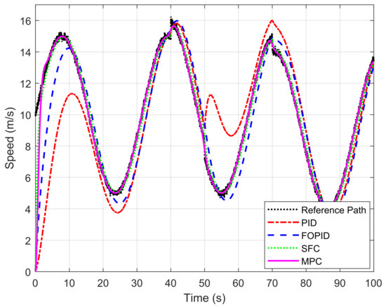
Figure 17.
Performance comparison of various motion control techniques for following a sinusoidal path with dynamic disturbances.
6. Conclusions
This paper presents an integrated framework for autonomous robotic navigation that combines three key components: environment mapping, path planning, and motion control. The performance of the proposed framework is evaluated on four distinct occupancy maps, including binary and probabilistic maps. Based on the performance evaluation of path planning algorithms on four occupancy map scenarios, Hybrid A* has achieved the optimal path with the shortest length from start to node of 131.86 m for Case 1, 726.05 m for Case 2, 40.29 m for Case 3, and 700.82 m for Case 4. The A* with Euclidean and Chebyshev heuristics also achieved the shortest paths in Case 1 with 129.30 m, Case 2 with 735.46 m and 737.22 m, and Case 3 with 39.59 m. However, all other compared techniques, such as PRM and RRT-based algorithms, have achieved longer paths. Furthermore, based on the performance evaluation of motion control techniques on the tracking sinusoidal path, MPC has outperformed all other compared controllers, such as PID, FOPID, and SFC, with the lowest tracking errors in terms of MAE, RMSE, and IAE of 0.09, 0.59, and 9.89, respectively. In addition, the numerical analysis, in terms of computational time and safety margin, also revealed that the A* algorithm with various cost functions achieved the shortest computational times, ranging from 0.006 to 0.165 s, with safety margins between 1.24 and 1.52 m. In contrast, the RRT, RRT*, and BiRRT algorithms have a longer computation time, ranging from 3 to 7 s, but offer the highest safety margins, up to 1.58 m. The Hybrid A* algorithm has yielded moderate computational times, ranging from 0.325 to 136.39 s, and a safety margin of 1.29 to 3.28 m, maintaining a competitive trade-off between computational effort and path safety.
These results demonstrate that the integrated framework offers an adaptable solution for robotic navigation, with the Hybrid A* and MPC being the optimal choices for path planning and motion control. However, a limitation of the present work is that the integration between path planning and motion control is represented using a predefined sinusoidal path under ideal conditions and in the presence of dynamic disturbances, rather than through direct closed-loop interaction. Therefore, future work will focus on integrating path planners and motion controllers in real-world environments that account for sensing noise, dynamic objects, and SLAM drift, aiming to achieve fully autonomous, adaptive navigation.
Author Contributions
Conceptualization, K.B. and A.P.S.; methodology, K.B. and A.P.S.; software, N.B.S. and A.R.; validation, K.B. and A.P.S.; formal analysis, K.B. and R.I.; investigation, K.B. and R.I.; resources, K.B. and R.I.; data curation, N.B.S. and A.R.; writing—original draft preparation, K.B. and A.P.S.; writing—review and editing, R.I., N.B.S. and A.R.; visualization, A.P.S.; supervision, A.P.S.; project administration, R.I., N.B.S. and A.R.; funding acquisition, R.I., N.B.S. and A.R. All authors have read and agreed to the published version of the manuscript.
Funding
This research received no external funding.
Data Availability Statement
The raw data supporting the conclusions of this article will be made available by the authors on request.
Conflicts of Interest
The authors declare no conflicts of interest.
Abbreviations
The following abbreviations are used in this manuscript:
| ARA* | Anytime Repairing A* |
| BiRRT | Bidirectional Rapidly Exploring Random Tree |
| BIT | Batch Informed Trees |
| FOPID | Fractional-order PID |
| IAE | Integral of Absolute Error |
| LiDAR | Light Detection and Ranging |
| MAE | Mean Absolute Error |
| MPC | Model Predictive Control |
| PID | Proportional-Integral-Derivative |
| PRM | Probabilistic Roadmaps |
| RMSE | Root Mean Square Error |
| ROS | Robot Operating System |
| RRT | Rapidly Exploring Random Tree |
| RTAB | Real-Time Appearance-Based Mapping |
| SFC | State Feedback Control |
| SLAM | Simultaneous Localisation and Mapping |
References
- Chen, W.; Chi, W.; Ji, S.; Ye, H.; Liu, J.; Jia, Y.; Yu, J.; Cheng, J. A survey of autonomous robots and multi-robot navigation: Perception, planning and collaboration. Biomim. Intell. Robot. 2025, 5, 100203. [Google Scholar] [CrossRef]
- Liu, L.; Wang, X.; Yang, X.; Liu, H.; Li, J.; Wang, P. Path planning techniques for mobile robots: Review and prospect. Expert Syst. Appl. 2023, 227, 120254. [Google Scholar] [CrossRef]
- Crespo, J.; Castillo, J.C.; Mozos, O.M.; Barber, R. Semantic information for robot navigation: A survey. Appl. Sci. 2020, 10, 497. [Google Scholar] [CrossRef]
- Lluvia, I.; Lazkano, E.; Ansuategi, A. Active mapping and robot exploration: A survey. Sensors 2021, 21, 2445. [Google Scholar] [CrossRef]
- Sánchez-Ibáñez, J.R.; Pérez-del Pulgar, C.J.; García-Cerezo, A. Path planning for autonomous mobile robots: A review. Sensors 2021, 21, 7898. [Google Scholar] [CrossRef]
- Aggarwal, S.; Kumar, N. Path planning techniques for unmanned aerial vehicles: A review, solutions, and challenges. Comput. Commun. 2020, 149, 270–299. [Google Scholar] [CrossRef]
- Zhang, H.y.; Lin, W.m.; Chen, A.x. Path planning for the mobile robot: A review. Symmetry 2018, 10, 450. [Google Scholar] [CrossRef]
- Tang, Y.; Zakaria, M.A.; Younas, M. Path planning trends for autonomous mobile robot navigation: A review. Sensors 2025, 25, 1206. [Google Scholar] [CrossRef]
- Tzafestas, S.G. Mobile robot control and navigation: A global overview. J. Intell. Robot. Syst. 2018, 91, 35–58. [Google Scholar] [CrossRef]
- Xiao, X.; Liu, B.; Warnell, G.; Stone, P. Motion planning and control for mobile robot navigation using machine learning: A survey. Auton. Robot. 2022, 46, 569–597. [Google Scholar] [CrossRef]
- Hornung, A.; Wurm, K.M.; Bennewitz, M.; Stachniss, C.; Burgard, W. OctoMap: An efficient probabilistic 3D mapping framework based on octrees. Auton. Robot. 2013, 34, 189–206. [Google Scholar] [CrossRef]
- Wang, H.; Zhang, G.; Cao, H.; Hu, K.; Wang, Q.; Deng, Y.; Gao, J.; Tang, Y. Geometry-Aware 3D Point Cloud Learning for Precise Cutting-Point Detection in Unstructured Field Environments. J. Field Robot. 2025, 42, 3063–3076. [Google Scholar] [CrossRef]
- Labbé, M.; Michaud, F. RTAB-Map as an open-source lidar and visual simultaneous localization and mapping library for large-scale and long-term online operation. J. Field Robot. 2019, 36, 416–446. [Google Scholar] [CrossRef]
- Mur-Artal, R.; Tardós, J.D. Orb-slam2: An open-source slam system for monocular, stereo, and rgb-d cameras. IEEE Trans. Robot. 2017, 33, 1255–1262. [Google Scholar] [CrossRef]
- Campos, C.; Elvira, R.; Rodríguez, J.J.G.; Montiel, J.M.; Tardós, J.D. Orb-slam3: An accurate open-source library for visual, visual–inertial, and multimap slam. IEEE Trans. Robot. 2021, 37, 1874–1890. [Google Scholar] [CrossRef]
- Yilmaz, Ö.; KarakuŞ, F. Stereo and Kinect Fusion for continuous 3D reconstruction and visual odometry. Turk. J. Electr. Eng. Comput. Sci. 2016, 24, 2756–2770. [Google Scholar] [CrossRef]
- Qin, H.; Shao, S.; Wang, T.; Yu, X.; Jiang, Y.; Cao, Z. Review of autonomous path planning algorithms for mobile robots. Drones 2023, 7, 211. [Google Scholar] [CrossRef]
- Gul, F.; Mir, I.; Abualigah, L.; Sumari, P.; Forestiero, A. A consolidated review of path planning and optimization techniques: Technical perspectives and future directions. Electronics 2021, 10, 2250. [Google Scholar] [CrossRef]
- Borkar, K.K.; Aljrees, T.; Pandey, S.K.; Kumar, A.; Singh, M.K.; Sinha, A.; Singh, K.U.; Sharma, V. Stability analysis and navigational techniques of wheeled mobile robot: A review. Processes 2023, 11, 3302. [Google Scholar] [CrossRef]
- Iqbal, M.; Zhang, K.; Iqbal, S.; Tariq, I. A fast and reliable Dijkstra algorithm for online shortest path. Int. J. Comput. Sci. Eng. 2018, 5, 24–27. [Google Scholar] [CrossRef]
- Erke, S.; Bin, D.; Yiming, N.; Qi, Z.; Liang, X.; Dawei, Z. An improved A-Star based path planning algorithm for autonomous land vehicles. Int. J. Adv. Robot. Syst. 2020, 17, 1729881420962263. [Google Scholar] [CrossRef]
- Eskandarian, A.; Wu, C.; Sun, C. Research advances and challenges of autonomous and connected ground vehicles. IEEE Trans. Intell. Transp. Syst. 2019, 22, 683–711. [Google Scholar] [CrossRef]
- Bagad, P.; Dahatonde, P.; Gagare, R.; Athare, I.; Ghule, G. Optimizing Pathfinding in Dynamic Environments: A Comparative Study of A* and D-Lite Algorithms. In Proceedings of the 2024 IEEE Pune Section International Conference (PuneCon), Pune, India, 13–15 December 2024; pp. 1–11. [Google Scholar]
- Sandakalum, T.; Ang, M.H., Jr. Motion planning for mobile manipulators—a systematic review. Machines 2022, 10, 97. [Google Scholar] [CrossRef]
- Chen, G.; Luo, N.; Liu, D.; Zhao, Z.; Liang, C. Path planning for manipulators based on an improved probabilistic roadmap method. Robot.-Comput.-Integr. Manuf. 2021, 72, 102196. [Google Scholar]
- Ravankar, A.A.; Ravankar, A.; Emaru, T.; Kobayashi, Y. HPPRM: Hybrid potential based probabilistic roadmap algorithm for improved dynamic path planning of mobile robots. IEEE Access 2020, 8, 221743–221766. [Google Scholar] [CrossRef]
- Qiao, L.; Luo, X.; Luo, Q. An optimized probabilistic roadmap algorithm for path planning of mobile robots in complex environments with narrow channels. Sensors 2022, 22, 8983. [Google Scholar] [CrossRef]
- Wei, K.; Ren, B. A method on dynamic path planning for robotic manipulator autonomous obstacle avoidance based on an improved RRT algorithm. Sensors 2018, 18, 571. [Google Scholar] [CrossRef]
- Ma, G.; Duan, Y.; Li, M.; Xie, Z.; Zhu, J. A probability smoothing Bi-RRT path planning algorithm for indoor robot. Future Gener. Comput. Syst. 2023, 143, 349–360. [Google Scholar]
- Zhang, H.; Wang, Y.; Zheng, J.; Yu, J. Path planning of industrial robot based on improved RRT algorithm in complex environments. IEEE Access 2018, 6, 53296–53306. [Google Scholar] [CrossRef]
- Wang, J.; Chi, W.; Li, C.; Wang, C.; Meng, M.Q.H. Neural RRT*: Learning-based optimal path planning. IEEE Trans. Autom. Sci. Eng. 2020, 17, 1748–1758. [Google Scholar] [CrossRef]
- Gammell, J.D.; Barfoot, T.D.; Srinivasa, S.S. Batch informed trees (bit*): Informed asymptotically optimal anytime search. Int. J. Robot. Res. 2020, 39, 543–567. [Google Scholar] [CrossRef]
- Pérez-Juárez, J.G.; García-Martínez, J.R.; Medina Santiago, A.; Cruz-Miguel, E.E.; Olmedo-García, L.F.; Barra-Vázquez, O.A.; Rojas-Hernández, M.A. Kinematic Fuzzy Logic-Based Controller for Trajectory Tracking of Wheeled Mobile Robots in Virtual Environments. Symmetry 2025, 17, 301. [Google Scholar] [CrossRef]
- Bingul, Z.; Gul, K. Intelligent-PID with PD feedforward trajectory tracking control of an autonomous underwater vehicle. Machines 2023, 11, 300. [Google Scholar] [CrossRef]
- Acosta, D.; Fariña, B.; Toledo, J.; Acosta, L. Improving mobile robot maneuver performance using fractional-order controller. Sensors 2023, 23, 3191. [Google Scholar] [CrossRef]
- Zhang, X.; Li, J.; Ma, Z.; Chen, D.; Zhou, X. Lateral trajectory tracking of self-driving vehicles based on sliding mode and fractional-order proportional-integral-derivative control. Actuators 2023, 13, 7. [Google Scholar]
- Wang, Z.; Sun, K.; Ma, S.; Sun, L.; Gao, W.; Dong, Z. Improved linear quadratic regulator lateral path tracking approach based on a real-time updated algorithm with fuzzy control and cosine similarity for autonomous vehicles. Electronics 2022, 11, 3703. [Google Scholar] [CrossRef]
- Villalba-Aguilera, E.; Blesa, J.; Ponsa, P. Model-based predictive control for position and orientation tracking in a multilayer architecture for a three-wheeled omnidirectional mobile robot. Robotics 2025, 14, 72. [Google Scholar]
- Chen, G.; Dong, W.; Peng, P.; Alonso-Mora, J.; Zhu, X. Continuous occupancy mapping in dynamic environments using particles. IEEE Trans. Robot. 2023, 40, 64–84. [Google Scholar] [CrossRef]
- Wang, Y.; Zhao, L.; Huang, S. Occupancy-slam: An efficient and robust algorithm for simultaneously optimizing robot poses and occupancy map. IEEE Trans. Robot. 2025, 41, 4057–4077. [Google Scholar] [CrossRef]
- Bingi, K.; Ibrahim, R.; Karsiti, M.N.; Hassan, S.M.; Harindran, V.R. Fractional-Order Systems and PID Controllers; Springer: Berlin/Heidelberg, Germany, 2020; Volume 264. [Google Scholar]
- Singh, A.P.; Bingi, K. Applications of fractional-order calculus in robotics. Fractal Fract. 2024, 8, 403. [Google Scholar] [CrossRef]
- Bingi, K.; Rajanarayan Prusty, B.; Pal Singh, A. A review on fractional-order modelling and control of robotic manipulators. Fractal Fract. 2023, 7, 77. [Google Scholar] [CrossRef]
- Popescu, M.; Mronga, D.; Bergonzani, I.; Kumar, S.; Kirchner, F. Experimental investigations into using motion capture state feedback for real-time control of a humanoid robot. Sensors 2022, 22, 9853. [Google Scholar] [CrossRef] [PubMed]
- Benotsmane, R.; Kovács, G. Optimization of energy consumption of industrial robots using classical PID and MPC controllers. Energies 2023, 16, 3499. [Google Scholar] [CrossRef]
Disclaimer/Publisher’s Note: The statements, opinions and data contained in all publications are solely those of the individual author(s) and contributor(s) and not of MDPI and/or the editor(s). MDPI and/or the editor(s) disclaim responsibility for any injury to people or property resulting from any ideas, methods, instructions or products referred to in the content. |
© 2025 by the authors. Licensee MDPI, Basel, Switzerland. This article is an open access article distributed under the terms and conditions of the Creative Commons Attribution (CC BY) license (https://creativecommons.org/licenses/by/4.0/).