Finite-Time Synchronization of Fractional-Order Complex-Valued Multi-Layer Network via Adaptive Quantized Control Under Deceptive Attacks

Abstract

This article investigates the problem of finite-time synchronization of fractional-order complex-valued random multi-layer networks without decomposing them into two real-valued systems. Firstly, by promoting real-valued signum functions, sign functions on the complex-valued domain are introduced. Simultaneously, quantization functions in the complex-valued domain are also introduced, and several related formulas for sign functions and quantization functions in complex-valued domain are established. Under the framework of the given sign function and quantization function, an adaptive quantized control scheme with or without deception attacks is designed. According to the finite-time theorem, Lyapunov function, and graph theory methods, some sufficient criteria for realizing finite-time synchronization in complex-valued fractional-order multi-layer networks have been obtained. Furthermore, the setting time of finite-time synchronization is effectively evaluated. Eventually, the reliability of our results and the practicality of control strategies are verified through numerical examples.

1. Introduction

In recent years, loads of practical systems have been represented by single-layer complex networks, for instance, transportation networks [1], power networks [2] and the World Wide Web [3]. Nevertheless, the above research results describe complex single-layer networks and are unable to really regard the interactivities between networks in actual life. For instance, in transportation networks, multiple types of transportation, such as subways, buses, and taxis, coexist [1]. In social networks, people who use different social methods, such as phone, QQ, WeChat, etc., can be divided into different network layers [4]. These are composed of multi-layer networks (MLNs), which can better describe multiple relationships. Regarding the complicated interactions among network layers, MLNs have arisen at the historic moment and become an important research subfield little by little in the network science field.

It is noteworthy noting that most existing research on MLNs focuses on integer-order MLNs. However, traditional integer-order integral models are complex and, therefore, cannot fully describe the dynamic characteristics of certain real-world systems. Fortunately, due to its infinite memory and heritable properties [5], fractional calculus is considered a significant improvement over integer-order MLNs. It has already been used in the fields of synchronization and control applications, for example, electromagnetic waves, viscoelastic rheology, dielectric polarization [6,7,8]. In real life, the rotating fluid and laser issues in the real world can be precisely described and effectively overcome based on complex-valued problems [9,10]. Unlike real-valued complex networks, complex-valued complex networks have intricate features and widespread applications. For instance, in the complex-valued domain, both the XOR problem and symmetry detection can be better tackled [11]. Even better, the transmission of the signal through complex-valued MLNs has superior resistance to attacks [12]. The synchronization problem of multiple fractional-order fuzzy complex-valued networks was studied by designing a fuzzy pinning control protocol in [13]. Considering the universal applicability of MLNs, some research on complex-valued stochastic MLNs has achieved significant results [14,15]. However, these are the results of integer-order complex-valued multi-layer networks. Further in-depth research is needed on fractional-order complex-valued MLNs (FOCVMLNs).

Synchronization describes the phenomenon in nature where multiple individuals eventually converge through certain interactions. Real life applications contain swarm performance of drones [16] and communication [17]. Due to the great research significance of synchronization in MLNs, the current synchronization types in MLNs can be classified as complete synchronization [18], intra-layer synchronization [19], inter-layer synchronization [20], cluster synchronization [21]. Due to the lifespan of some biological agents and machinery equipment in practical engineering applications, it is often expected that the network will realize synchronization within a finite time rather than infinite time. Furthermore, finite-time synchronization (FITS) has better robustness and interference suppression characteristics [22]. Some research results have been achieved on FITS of fractional-order real-valued MLNs [23,24]. Due to the excellent resistance of signals transmitted through complex-valued networks to attacks, fruitful results have been achieved so far [25,26,27]. The FITS problem of fractional-order complex-valued networks was discussed by putting forward feedback control strategies in [25,26]. However, the above research results are all about the FITS of fractional-order complex-valued single-layer networks. The research results on FOCVMLNs are not yet sufficient. Therefore, studying the FITS of FOCVMLNs is reasonable and meaningful.

Generally speaking, FOCVMLNs cannot synchronize through their own behavior or coupling forms, which requires some external control to be applied to networks. General control inputs include adaptive control, impulsive control, quantized control, etc. In addition, in the aforementioned control methods, the quantized control is both effective and economical. Signal quantization can be seen as mapping continuous signals to a finite set of discrete signals, which merely requires encryption and transmission of these discrete signals. It greatly reduces the signal interference and lowers control costs. A new quantized control strategy was devised to study the fixed-time synchronization of a replication-coupled network with external and random disturbances in [28]. A new quantized intermittent control strategy was designed to investigate the exponential synchronization problem of neural networks based on complex-valued memristors in [29]. In contrast to the feedback control with a fixed control gain, the control gain of adaptive control can regulate itself according to constantly changing node states, therefore seeking out the optimum control gain and optimizing control costs [30,31,32]. The FITS of fractional-order complex-valued networks was discussed by devising adaptive control strategies in [30,31]. The FITS of fractional-order complex and neural networks were discussed by devising an adaptive quantized controller (AQC) in [24,33]. Nevertheless, there is currently a shortage of FITS results for AQC protocol in complex-valued domains. Hence, it is of vital importance to consider studying the FITS of FOCVMLNs under the AQC strategy.

Presently, with the widespread application and development of network communication technology, network security issues cannot be ignored. During the synchronization process, the network control systems will inevitably suffer from some malicious intrusions and random attacks, which commonly lead to a decline in network behavior or interruptions in realizing synchronization targets of MLNs by coupling. Generally speaking, cyber-attacks can be approximately classified as two types: denial-of-service attacks (DoS attacks) and deceptive attacks (DPAs). DoS attacks disrupt the communication channels between nodes in the network by taking up network resources, thereupon then impeding the successful transmission of data packets [34,35]. DPAs infuse incorrect data into the communication channels of the network and alter data packages to destroy the wholeness of control signals, which is extremely covert and not easy to prevent. It deserves the attention of researchers. Two kinds of event-triggered control strategies were designed to investigate the event-triggered synchronization of fractional-order networks with DPAs [36,37]. However, there are currently no relevant outcomes on the FITS of FOCVMLNs under DPAs.

Inspired by the above, a new AQC strategy is proposed in a complex-valued domain. In addition, due to the features of network information sharing, the control systems of the network are susceptible to malignant network attacks. Enlightened by these discussions, this article investigates the FITS problem of FOCVMLNs under DPAs. The major contributions of this text are as below.

(1)

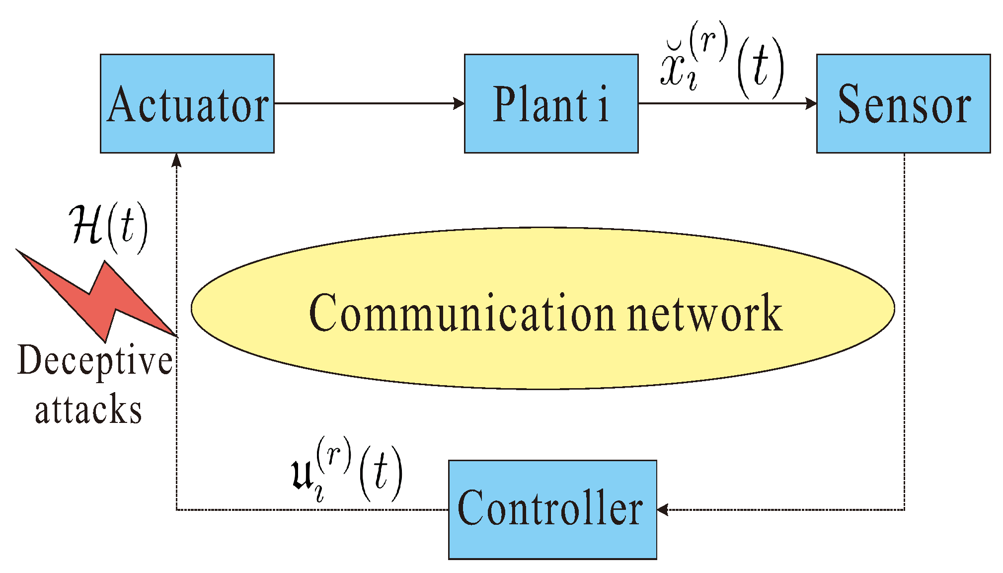
The designed AQC strategy combines the merits of adaptive control and quantized control. Considering the vulnerability of network systems to stochastic DPAs, a random variable that follows the Bernoulli distribution has been designed, which is more practical.

(2)

This article introduces new sign functions and quantization functions in the complex domain and establishes some related formulas for the complex-valued domain. It studies the FITS of FOCVMLNs, and the settling time of FITS is sufficiently evaluated.

(3)

A sufficient criterion for FITS of FOCVMLNs under stochastic DPAs is designed based on Lyapunov functions and graph theory methods. The numerical simulation presented at the end demonstrates the dependability of theoretical deductions.

Notations:  ${\mathbb{R}}_{+}$ is the set composed of all non-negative constants. ${\mathbb{R}}^n$ represents the space consisted of total n-dimensional real vectors. $\mathbb{C}$ and ${\mathbb{C}}^{n\times n}$ separately express the set of total complex numbers and a space consisting of total n-dimensional complex vectors. $\aleph =\{1,2,\dots ,\mathcal{N}\}$ and $\Re =\{1,2,\dots ,\mathcal{L}\}$ individually mean the set of vertexes and the set of layers. For any $\mathrm{k}=x+iy\in \mathbb{C}$, $\overline{\mathrm{k}}=x-iy$ signifies the conjugate of $\mathrm{k}$, ${|\mathrm{k}|}_1=|x|+|y|$, ${|\mathrm{k}|}_2=\sqrt{\overline{\mathrm{k}}\mathrm{k}}$, wherein $i^2=-1$, $x,y\in \mathbb{R}$ and $\mathrm{Re}\left(\mathrm{k}\right)=x$, $\mathrm{Im}\left(\mathrm{k}\right)=y$. For arbitrary $\mathbb{K}=({\mathrm{k}}_1,{\mathrm{k}}_2,\dots ,{\mathrm{k}}_n)\in {\mathbb{C}}^n$, ${\mathbb{K}}^H$ denotes its conjugate transposition, ${||\mathbb{K}||}_1={\displaystyle \sum _{𝚤=1}^{\mathcal{N}}}{|{\mathrm{k}}_{𝚤}|}_1$, ${||\mathbb{K}||}_2=({\displaystyle \sum _{𝚤=1}^{\mathcal{N}}}|{\mathrm{k}}_{𝚤}{{|}^2)}^{{\displaystyle \frac{1}{2}}}$. Assuming ${\mathbb{C}}^{n\times n}$ represents the set of total n-dimensional complex-valued matrices. ${\mathrm{I}}_n$ stands for the $n\times n$ unit matrix. ⊗ denotes Kronecker product. ${\lambda }_{\max }\left(A\right)$ signifies the maximum eigenvalue of real symmetric matrix A. $\mathbb{P}\{\Psi \}$ denotes the probability operator of event $\Psi$. $\mathbb{E}\{\Psi \}$ denotes the exception operator for an event $\Psi$.

2. Preliminaries and Problem Description

A. Algebraic Graph Theory

Consider a FOCVMLN undigraph  ${\mathcal{G}}^{\left(r\right)}=(\mathbb{V},{\mathcal{E}}^{\left(r\right)},{\mathcal{A}}^{\left(r\right)})$, wherein $\mathbb{V}=\{{\mathbb{V}}_1,{\mathbb{V}}_2,\dots ,{\mathbb{V}}_{\mathcal{N}}\}$ represents the set of vertexes, ${\mathcal{E}}^{\left(r\right)}\subseteq \mathbb{V}\times \mathbb{V}$ expresses the set of edges composed of vertexes. ${\mathcal{A}}^{\left(r\right)}={\left(a_{𝚤j}^{\left(r\right)}\right)}_{\mathcal{N}\times \mathcal{N}}(𝚤,j\in \aleph )$ denotes the adjacency matrix of ${\mathcal{G}}^{\left(r\right)}$, where $a_{𝚤j}^{\left(r\right)}=a_{j𝚤}^{\left(r\right)}>0(𝚤\ne j)$ when there is a link between vertex ı and vertex j in layer r, otherwise $a_{𝚤j}^{\left(r\right)}=0$. The corresponding Laplace matrix ${\mathfrak{L}}_{\mathcal{A}}^{\left(r\right)}={\left({\widehat{a}}_{𝚤j}^{\left(r\right)}\right)}_{\mathcal{N}\times \mathcal{N}}$ is ${\widehat{a}}_{𝚤j}^{\left(r\right)}={\widehat{a}}_{j𝚤}^{\left(r\right)}=-a_{𝚤j}^{\left(r\right)}<0(𝚤\ne j)$, and ${\widehat{a}}_{𝚤𝚤}^{\left(r\right)}={\displaystyle \sum _{j=1,j\ne 𝚤}^{\mathcal{N}}}{a}_{𝚤j}^{\left(r\right)}$.

B. Problem Description

The dynamic equation of FOCVMLN consists of an $\mathcal{L}(\mathcal{L}\ge 2)$-layer network with $\mathcal{N}$ nodes in each layer, as shown below.

$$\begin{array}{cc}& {}_{t_0}{}^{C}D_t^{\breve{\alpha }}{\breve{x}}_{𝚤}^{\left(r\right)}\left(t\right)=\mathfrak{f}\left({\breve{x}}_{𝚤}^{\left(r\right)}\left(t\right)\right)+c{\displaystyle \sum _{j=1}^{\mathcal{N}}}{a}_{𝚤j}^{\left(r\right)}\mathcal{P}({\breve{x}}_j^{\left(r\right)}\left(t\right)-{\breve{x}}_{𝚤}^{\left(r\right)}\left(t\right))\hfill \\ & +d{\displaystyle \sum _{k=1}^{\mathcal{L}}}{b}_{rk}\mathcal{Q}({\breve{x}}_{𝚤}^{\left(k\right)}\left(t\right)-{\breve{x}}_{𝚤}^{\left(r\right)}\left(t\right))+{\mathfrak{u}}_{𝚤}^{\left(r\right)}\left(t\right),𝚤\in \aleph ,r\in \Re ,\hfill \end{array}$$

(1)

in which ${\breve{x}}_{𝚤}^{\left(r\right)}\left(t\right)={({\breve{x}}_{𝚤1}^{\left(r\right)}\left(t\right),{\breve{x}}_{𝚤2}^{\left(r\right)}\left(t\right),\dots ,{\breve{x}}_{𝚤n}^{\left(r\right)}\left(t\right))}^T\in {\mathbb{C}}^n$ represents the state vector of the ıth node in the rth layer, $\mathfrak{f}\left({\breve{x}}_{𝚤}^{\left(r\right)}\left(t\right)\right)=({\mathfrak{f}}_1\left({\breve{x}}_{𝚤}^{\left(r\right)}\left(t\right)\right),{\mathfrak{f}}_2\left({\breve{x}}_{𝚤}^{\left(r\right)}\left(t\right)\right),\dots ,{\mathfrak{f}}_n\left({\breve{x}}_{𝚤}^{\left(r\right)}\left(t\right)\right))\in {\mathbb{C}}^n$ expresses a sleek nonlinear vector function, c and d separately show the coupling weights of intra-layer and inter-layer. $\mathcal{P}=\mathbf{diag}({\mathcal{P}}_1,{\mathcal{P}}_2,\dots ,{\mathcal{P}}_n)\in {\mathbb{C}}^{n\times n}$ means the coupling matrix of intra-layer. $\mathcal{Q}=\mathbf{diag}({\mathcal{Q}}_1,{\mathcal{Q}}_2,\dots ,{\mathcal{Q}}_n)\in {\mathbb{C}}^{n\times n}$ shows the coupling matrix between vertexes in the inter-layer. $\mathcal{B}={\left(b_{rk}\right)}_{\mathcal{L}\times \mathcal{L}}$ is the corresponding adjacency matrix between nodes in the rth and the kth layer. ${\mathfrak{L}}_{\mathcal{B}}={\left({\widehat{b}}_{rk}\right)}_{\mathcal{L}\times \mathcal{L}}$ is the Laplace matrix of inter-layer, which is defined as ${\widehat{b}}_{rk}={\widehat{b}}_{kr}=-b_{rk}<0(r\ne k)$, and ${\widehat{b}}_{rr}={\displaystyle \sum _{k=1,k\ne r}^{\mathcal{L}}}{b}_{rk}>0$. The initial condition for system (1) is ${\mathcal{X}}^{\left(r\right)}\left(0\right)={({\left({\breve{x}}_1^{\left(r\right)}\left(0\right)\right)}^T,{\left({\breve{x}}_2^{\left(r\right)}\left(0\right)\right)}^T,\dots ,{\left({\breve{x}}_{\mathcal{N}}^{\left(r\right)}\left(0\right)\right)}^T)}^T\in {\mathbb{C}}^{\mathcal{N}n}$.

Definition 1

([8,38]). The Caputo fractional-order derivative of order $\breve{\alpha }>0$ for a function $\varphi \left(t\right):[t_0,+\infty )\to \mathbb{C}$ is given by

$${}_{t_0}{}^{C}D_t^{\breve{\alpha }}\varphi \left(t\right)={\displaystyle \frac{1}{\Gamma (1-\breve{\alpha })}}{\int }_{t_0}^t{\displaystyle \frac{{\varphi }^{\prime }\left(\breve{\omega }\right)}{{(t-\breve{\omega })}^{\breve{\alpha }}}}d\breve{\omega },0<\breve{\alpha }<1.$$

Definition 2

([8,38]). For an integrable function $\varphi \left(t\right):[t_0,+\infty )\to \mathbb{C}$, the fractional integral of it with order $\breve{\alpha }$ is given by

$${}_{t_0}I_t^{\breve{\alpha }}\varphi \left(t\right)={\displaystyle \frac{1}{\Gamma \left(\breve{\alpha }\right)}}{\int }_{t_0}^t{(t-\breve{\omega })}^{\breve{\alpha }-1}\varphi \left(\breve{\omega }\right)d\breve{\omega },0<\breve{\alpha }<1,$$

where $t\ge t_0$, $\Gamma \left(\breve{\alpha }\right)={\int }_0^{\infty }{\breve{\omega }}^{\breve{\alpha }-1}{g}^{-\breve{\omega }}d\breve{\omega }$.

Lemma 1

([39]). If $x\left(t\right)\in {\mathbb{C}}^n$ is a continuous and analytic function, then for any $t\ge t_0$,

$${}_{t_0}{}^{C}D_t^{\breve{\alpha }}{x}^H\left(t\right)x\left(t\right)\le x^H\left(t\right){}_{t_0}{}^{C}D_t^{\breve{\alpha }}x\left(t\right)+\left({}_{t_0}{}^{C}D_t^{\breve{\alpha }}{x}^H\left(t\right)\right)x\left(t\right),0<\breve{\alpha }<1.$$

Lemma 2

([8,38]). Suppose that function $\varphi \left(t\right):[t_0,+\infty )\to \mathbb{C}$ is consecutive differentiable, then for all $t\in [t_0,+\infty )$,

$${}_{t_0}I_t^{\breve{\alpha }}{}_{t_0}{}^{C}D_t^{\breve{\alpha }}\varphi \left(t\right)=\varphi \left(t\right)-\varphi \left(t_0\right),0<\breve{\alpha }<1.$$

Lemma 3

([25]). For any $\mathfrak{a}\in \mathbb{C}$,

$$\mathfrak{a}+\overline{\mathfrak{a}}=2Re\left(\mathfrak{a}\right)\le {2|\mathfrak{a}|}_2\le 2{|\mathfrak{a}|}_1.$$

Definition 3

([26]). For any $\upsilon \in \mathbb{C}$, $\left[\upsilon \right]=\mathbf{sign}\left(\mathrm{Re}\right(\upsilon \left)\right)+i\mathbf{sign}\left(\mathrm{Im}\right(\upsilon \left)\right)$ is called the signum function of υ. For any $\mu \in {\mathbb{C}}^n$, $\left[\mu \right]={(\mathbf{sign}\left(\mathrm{Re}\left({\mu }_1\right)\right)+i\mathbf{sign}\left(\mathrm{Im}\left({\mu }_1\right)\right),\dots ,\mathbf{sign}\left(\mathrm{Re}\left({\mu }_n\right)\right)+i\mathbf{sign}\left(\mathrm{Im}\left({\mu }_n\right)\right))}^T$ is called the signum function of μ.

Lemma 4

([26]). Assume that $\upsilon \left(t\right)\in \mathbb{C}$, $\mu \left(t\right)\in {\mathbb{C}}^n$, then

(1) 

${\upsilon }^H\left(t\right)\left[\mu \left(t\right)\right]+{\left[\mu \left(t\right)\right]}^H\upsilon \left(t\right)\le {2||\upsilon \left(t\right)||}_1$.

(2) 

${\mu }^H\left(t\right)\left[\mu \left(t\right)\right]+{\left[\mu \left(t\right)\right]}^H\mu \left(t\right)={2||\mu \left(t\right)||}_1\ge {2||\mu \left(t\right)||}_2$.

(3) 

${}_{t_0}{}^{C}D_t^{\breve{\alpha }}({\left[\mu \left(t\right)\right]}^H\mu \left(t\right)+{\mu }^H\left(t\right)\left[\mu \left(t\right)\right])\le {\left[\mu \left(t\right)\right]}^H{}_{t_0}{}^{C}D_t^{\breve{\alpha }}\mu \left(t\right)+\left({}_{t_0}{}^{C}D_t^{\breve{\alpha }}{\mu }^H\left(t\right)\right)\left[\mu \left(t\right)\right]$.

(4) 

${\left[\mu \left(t\right)\right]}^H\left[\mu \left(t\right)\right]={||\left[\mu \left(t\right)\right]||}_1$.

Lemma 5

([26]). Assume that $\mathcal{V}\left(t\right):[t_0,+\infty )\to {\mathbb{R}}_{+}$ is a continuous positive definite function, if there exists a constant $\xi >0$ such that

$${}_{t_0}{}^{C}D_t^{\breve{\alpha }}\mathcal{V}\left(t\right)\le -\xi ,\mathcal{V}\left(t\right)\in {\mathbb{R}}_{+}\backslash \left\{0\right\},$$

then $\mathcal{V}\left(t\right)=0$ for all $t\ge t^{★}$, where $0<\breve{\alpha }<1$, $t^{★}=t_0+{\left({\displaystyle \frac{\Gamma (\breve{\alpha }+1)V\left(t_0\right)}{\xi }}\right)}^{{\displaystyle \frac{1}{\breve{\alpha }}}}$.

The synchronization objective equation of network (1) is described as

$$\begin{array}{cc}& {}_{t_0}{}^{C}D_t^{\breve{\alpha }}{s}^{\left(r\right)}\left(t\right)=\mathfrak{f}\left(s^{\left(r\right)}\left(t\right)\right),r\in \Re ,\hfill \end{array}$$

(2)

wherein $0<\breve{\alpha }<1$, $s^{\left(r\right)}\left(t\right)=(s_1^{\left(r\right)},s_2^{\left(r\right)},\dots ,s_n^{\left(r\right)})\in {\mathbb{C}}^n$.

Definition 4

([40]). The system (1) is called to realize FITS provided that there exists a constant $T\ge 0$ related to the initial value such that

$$\underset{t\to T}{lim}||{\breve{x}}_{𝚤}^{\left(r\right)}\left(t\right)-s^{\left(r\right)}\left(t\right)||=0,𝚤\in \aleph ,r\in \Re ,$$

and $||{\breve{x}}_{𝚤}^{\left(r\right)}\left(t\right)-s^{\left(r\right)}\left(t\right)||=0$ for all $t\ge T$, where

$$T=\inf \{T\ge 0:{\breve{x}}_{𝚤}^{\left(r\right)}\left(t\right)=s^{\left(r\right)}\left(t\right)\mathrm{for}t\ge T\}$$

is known as the settling time of synchronization.

Assumption 1.

There exists a constant $L_{\mathfrak{f}}>0$ such that

$$||\mathfrak{f}\left(\mathrm{y}\right)-{\mathfrak{f}\left(\mathrm{z}\right)||}_2\le L_{\mathfrak{f}}||\mathrm{y}-{\mathrm{z}||}_2,\mathrm{y},\mathrm{z}\in {\mathbb{C}}^n.$$

Define the state error as ${ϵ}_{𝚤}^{\left(r\right)}\left(t\right)={\breve{x}}_{𝚤}^{\left(r\right)}\left(t\right)-s^{\left(r\right)}\left(t\right)$, the error system is express as below.

$$\begin{array}{cc}& {}_{t_0}{}^{C}D_t^{\breve{\alpha }}{ϵ}_{𝚤}^{\left(r\right)}\left(t\right)=\tilde{\mathfrak{f}}\left({ϵ}_{𝚤}^{\left(r\right)}\left(t\right)\right)+c{\displaystyle \sum _{j=1}^{\mathcal{N}}}{a}_{𝚤j}^{\left(r\right)}\mathcal{P}({ϵ}_j^{\left(r\right)}\left(t\right)-{ϵ}_{𝚤}^{\left(r\right)}\left(t\right))\hfill \\ & +d{\displaystyle \sum _{k=1}^{\mathcal{L}}}{b}_{rk}\mathcal{Q}({ϵ}_{𝚤}^{\left(k\right)}\left(t\right)-{ϵ}_{𝚤}^{\left(r\right)}\left(t\right))+{\mathfrak{u}}_{𝚤}^{\left(r\right)}\left(t\right),𝚤\in \aleph ,r\in \Re ,\hfill \end{array}$$

(3)

where $\tilde{\mathfrak{f}}\left({ϵ}_{𝚤}^{\left(r\right)}\left(t\right)\right)=\mathfrak{f}\left({\breve{x}}_{𝚤}^{\left(r\right)}\left(t\right)\right)-\mathfrak{f}\left(s^{\left(r\right)}\left(t\right)\right)$.

3. Main Results

A. FITS with cyber attack

In this part, we will investigate the FITS of FOMLNs under cyber-attacks. In recent years, cyber-attacks have occurred frequently, and network security has turned into a hot research topic. When the network communication channel is attacked, the controller is unable to accept the correct state information. Based on previous research results [36,37], we design an adaptive quantized control strategy under random cyber attack as below.

$$\begin{array}{c}\hfill {\mathfrak{u}}_{𝚤}^{\left(r\right)}\left(t\right)=\varpi \left(t\right)\mathcal{H}\left(t\right)+(1-\varpi \left(t\right)){\phi }_{𝚤}^{\left(r\right)}\left(t\right),𝚤\in \aleph ,r\in \Re ,\end{array}$$

(4)

where $\mathcal{H}\left(t\right)$ is the stochastic DPAs signal. $\varpi \left(t\right)$ denotes a Bernoulli random variable, which satisfies $\mathbb{P}\left\{\varpi \right(t)=1\}=\varpi$, $\mathbb{P}\left\{\varpi \right(t)=0\}=1-\varpi$, $\varpi \in (0,1)$ is a known constant, and $\mathbb{E}\left\{\varpi \left(t\right)\right\}=\mathbb{E}\left\{\varpi {\left(t\right)}^2\right\}=\varpi$. ${\phi }_{𝚤}^{\left(r\right)}\left(t\right)$ is a controller that receives normal signals, which is designed as below.

$$\begin{array}{c}\hfill {\phi }_{𝚤}^{\left(r\right)}\left(t\right)=\left\{\begin{array}{ccc}& {\displaystyle -k_{𝚤}^{\left(r\right)}\left(t\right)\mathfrak{q}\left({ϵ}_{𝚤}^{\left(r\right)}\left(t\right)\right)-{\eta }^{\left(r\right)}\mathbf{sign}\left(\mathfrak{q}\left({ϵ}_{𝚤}^{\left(r\right)}\left(t\right)\right)\right)-\frac{\Lambda \mathfrak{q}\left({ϵ}_{𝚤}^{\left(r\right)}\left(t\right)\right)}{||{ϵ}_{𝚤}^{\left(r\right)}\left(t\right){||}^2},}\hfill & ||{ϵ}_{𝚤}^{\left(r\right)}\left(t\right)||\ne 0\hfill \\ & 0,\hfill & ||{ϵ}_{𝚤}^{\left(r\right)}\left(t\right)||=0.\hfill \end{array}\right.\end{array}$$

(5)

$$\begin{array}{c}\hfill {}_{t_0}{}^{C}D_t^{\breve{\alpha }}{k}_{𝚤}^{\left(r\right)}\left(t\right)=\epsilon (1-\varpi \left(t\right))(1-\chi ){\left({ϵ}_{𝚤}^{\left(r\right)}\left(t\right)\right)}^H{ϵ}_{𝚤}^{\left(r\right)}\left(t\right),\end{array}$$

(6)

where $k_{𝚤}^{\left(r\right)}\left(t\right)$ represents the adaptive control gain, $\Lambda \in {\mathbb{R}}_{+}$, $\mathfrak{q}\left({ϵ}_{𝚤}^{\left(r\right)}\left(t\right)\right)={(\widehat{\mathfrak{q}}\left({ϵ}_{𝚤1}^{\left(r\right)}\left(t\right)\right),\widehat{\mathfrak{q}}\left({ϵ}_{𝚤2}^{\left(r\right)}\left(t\right)\right),\dots ,\widehat{\mathfrak{q}}\left({ϵ}_{𝚤n}^{\left(r\right)}\left(t\right)\right))}^T$, where $\widehat{\mathfrak{q}}\left({ϵ}_{𝚤l}^{\left(r\right)}\left(t\right)\right)=\breve{\mathfrak{q}}\left(\mathrm{Re}\left({ϵ}_{𝚤l}^{\left(r\right)}\left(t\right)\right)\right)+i\breve{\mathfrak{q}}\left(\mathrm{Im}\left({ϵ}_{𝚤l}^{\left(r\right)}\left(t\right)\right)\right)$, wherein $l=1,2,\dots ,n$, $\mathbf{sign}\left(\mathfrak{q}\left({ϵ}_{𝚤}^{\left(r\right)}\left(t\right)\right)\right)=(\left[\widehat{\mathfrak{q}}\left({ϵ}_{𝚤1}^{\left(r\right)}\left(t\right)\right)\right],\left[\widehat{\mathfrak{q}}\left({ϵ}_{𝚤2}^{\left(r\right)}\left(t\right)\right)\right],\dots ,\left[\widehat{\mathfrak{q}}\left({ϵ}_{𝚤n}^{\left(r\right)}\left(t\right)\right)\right])$.

$$\begin{array}{c}\hfill \breve{\mathfrak{q}}\left(\mu \right)=\left\{\begin{array}{ccc}& {\wp }_{\iota },\hfill & {\displaystyle \frac{1}{1+\chi }{\wp }_{\iota }<\mu \le \frac{1}{1-\chi }{\wp }_{\iota },}\hfill \\ & 0,\hfill & \mu =0,\hfill \\ & -\breve{\mathfrak{q}}(-\mu ),\hfill & \mu <0,\hfill \end{array}\right.\end{array}$$

(7)

wherein $\zeta =\{\pm {\wp }_{\iota }:{\wp }_{\iota }={\varrho }^{\iota }{\wp }_0,\iota =0,\pm 1,\pm 2,\dots \}\bigcup \left\{0\right\}({\wp }_0>0)$ represents the set of quantification levels. ${\displaystyle \chi =\frac{1-\varrho }{1+\varrho }}$ expresses the quantification step. $0<\varrho <1$ denotes the quantization density. Analysis according to [41], there has a Filippov solution $\sigma \in [-\chi ,\chi )$ meeting $\breve{\mathfrak{q}}\left(\mu \right)=(1+\sigma )\mu ,\mu \in \mathbb{R}$.

Remark 1.

The specific structure of cyber-attacks is shown in Figure 1. The sensor receives status information ${\breve{x}}_{𝚤}^{\left(r\right)}\left(t\right)$ from plant i and then transmits it to the controller. The controller ${\mathfrak{u}}_{𝚤}^{\left(r\right)}\left(t\right)$ sends control signals to the actuator through the communication network. During the signal transmission process, the attacker inputs an incorrect data packet $\mathcal{H}\left(t\right)$ to the control signal through the communication network. Then, the tampered signal is sent to plant i through the actuator, thus completing the deceptive attack process.

Remark 2.

Actually, the AQC controller (4) has the following two situations:

(1) 

When $\varpi \left(t\right)=1$, DPAs are active. At this time, the AQC (4) can only receive erroneous data packets $\mathcal{H}\left(t\right)$.

(2) 

When $\varpi \left(t\right)=0$, DPAs do not exist. At this moment, the AQC (4) can only receive rightful data packets ${\phi }_{𝚤}^{\left(r\right)}\left(t\right)$.

Assumption 2.

For the continuous function $\mathcal{H}(·):{\mathbb{R}}^n\to {\mathbb{R}}^n$, there is a constant ${\mathcal{H}}_1>0$ such that

$${||\mathcal{H}(·)||}_2\le {\mathcal{H}}_1.$$

Remark 3.

The FITS problem of complex dynamic networks was investigated by devising an AQC algorithm in [42], but it neither considers random DPAs nor the situation in the complex-valued domain in synchronization. The controller (4) in this article has been improved based on this. Considering the influence of complex variables and DPAs on FOMLNs, a new adaptive complex-valued quantized controller is designed. Not only can it effectively reduce bandwidth and signal transmission voltage, but it can also resist network DPAs and suppress external interference.

Denote

$${\mathfrak{L}}_{\mathcal{A}}=({\mathfrak{L}}_{\mathcal{A}}^{\left(1\right)},{\mathfrak{L}}_{\mathcal{A}}^{\left(2\right)},\dots ,{\mathfrak{L}}_{\mathcal{A}}^{\left(\mathcal{L}\right)}),$$

$${\lambda }_1={\lambda }_{\min }\left((c{\mathfrak{L}}_{\mathcal{A}}\otimes \mathcal{P})+{(c{\mathfrak{L}}_{\mathcal{A}}\otimes \mathcal{P})}^H\right),$$

$${\lambda }_2={\lambda }_{\min }\left({\mathrm{I}}_{\mathcal{N}}\otimes \left(d{\mathfrak{L}}_{\mathcal{B}}\otimes \mathcal{Q}+{(d{\mathfrak{L}}_{\mathcal{B}}\otimes \mathcal{Q})}^H\right)\right),$$

$${\lambda }_3={\lambda }_{\min }\left(2(1-\varpi )(1-\chi )(\Delta \otimes {\mathrm{I}}_{\mathcal{L}n})\right),$$

$$\xi =2\Lambda (1-\varpi )(1-\chi ).$$

Theorem 1.

Under Assumptions 1 and 2 and the control protocol (4), the system (1) realizes FITS if there is a constant $\eta >0$ satisfying

$$\begin{array}{c}\hfill {\displaystyle \eta >\frac{\varpi {\mathcal{H}}_1}{1-\varpi },\eta ={\min }_{r\in \mathcal{L}}\left\{{\eta }^{\left(r\right)}\right\},}\end{array}$$

(8)

where the setting time of FITS is estimated as

$$\begin{array}{c}\hfill T_1=t_0+{\left({\displaystyle \frac{\mathcal{V}\left(ϵ\left(t_0\right)\right)\Gamma (\breve{\alpha }+1)}{\xi }}\right)}^{{\displaystyle \frac{1}{\breve{\alpha }}}}.\end{array}$$

Proof. 

Construct the following Lyapunov functions.

$$\begin{array}{c}\hfill \mathcal{V}\left(ϵ\left(t\right)\right)={\displaystyle \sum _{r=1}^{\mathcal{L}}}{\displaystyle \sum _{𝚤=1}^{\mathcal{N}}}{\left({ϵ}_{𝚤}^{\left(r\right)}\left(t\right)\right)}^H{ϵ}_{𝚤}^{\left(r\right)}\left(t\right)+{\displaystyle \sum _{r=1}^{\mathcal{L}}}{\displaystyle \sum _{𝚤=1}^{\mathcal{N}}}{\displaystyle \frac{{(k_{𝚤}^{\left(r\right)}\left(t\right)-{\delta }_{𝚤}^{\ast })}^2}{\epsilon }},\end{array}$$

where ${\delta }_{𝚤}^{\ast }>0$ is the adaptive constant,

$$ϵ\left(t\right)={\left({\left({ϵ}^{\left(1\right)}\left(t\right)\right)}^T,{\left({ϵ}^{\left(2\right)}\left(t\right)\right)}^T,\dots ,{\left({ϵ}^{\left(\mathcal{L}\right)}\left(t\right)\right)}^T\right)}^T,$$

$${ϵ}^{\left(r\right)}\left(t\right)={\left({\left({ϵ}_1^{\left(r\right)}\left(t\right)\right)}^T,{\left({ϵ}_2^{\left(r\right)}\left(t\right)\right)}^T,\dots ,{\left({ϵ}_{\mathcal{N}}^{\left(r\right)}\left(t\right)\right)}^T\right)}^T.$$

For $ϵ\left(t\right)\in {\mathbb{C}}^{\mathcal{L}\mathcal{N}n}\backslash \left\{0^{\mathcal{L}\mathcal{N}n}\right\}$, with the help of Lemma 1,

$$\begin{array}{cc}\hfill \mathbb{E}\left\{{}_{t_0}{}^{C}D_t^{\breve{\alpha }}\mathcal{V}\left(ϵ\left(t\right)\right)\right\}\le & {\displaystyle \sum _{r=1}^{\mathcal{L}}}{\displaystyle \sum _{𝚤=1}^{\mathcal{N}}}\left({\left({ϵ}_{𝚤}^{\left(r\right)}\left(t\right)\right)}^H\tilde{\mathfrak{f}}\left({ϵ}_{𝚤}^{\left(r\right)}\left(t\right)\right)+{\tilde{\mathfrak{f}}}^H\left({ϵ}_{𝚤}^{\left(r\right)}\left(t\right)\right){ϵ}_{𝚤}^{\left(r\right)}\left(t\right)\right)\hfill \\ \hfill & +{\displaystyle \sum _{r=1}^{\mathcal{L}}}{\displaystyle \sum _{𝚤=1}^{\mathcal{N}}}{\displaystyle \sum _{j=1}^{\mathcal{N}}}({\left({ϵ}_{𝚤}^{\left(r\right)}\left(t\right)\right)}^{H}c{a}_{𝚤j}^{\left(r\right)}\mathcal{P}\left({ϵ}_j^{\left(r\right)}\left(t\right)-{ϵ}_{𝚤}^{\left(r\right)}\left(t\right)\right)\hfill \\ \hfill & +\overline{c{a}_{𝚤j}^{\left(r\right)}}{\mathcal{P}}^H\left({\left({ϵ}_j^{\left(r\right)}\left(t\right)\right)}^H-{\left({ϵ}_{𝚤}^{\left(r\right)}\left(t\right)\right)}^H\right){ϵ}_{𝚤}^{\left(r\right)}\left(t\right))\hfill \\ \hfill & +{\displaystyle \sum _{r=1}^{\mathcal{L}}}{\displaystyle \sum _{𝚤=1}^{\mathcal{N}}}{\displaystyle \sum _{k=1}^{\mathcal{L}}}({\left({ϵ}_{𝚤}^{\left(r\right)}\left(t\right)\right)}^{H}d{b}_{rk}\mathcal{Q}\left({ϵ}_{𝚤}^{\left(k\right)}\left(t\right)-{ϵ}_{𝚤}^{\left(r\right)}\left(t\right)\right)\hfill \\ \hfill & +\overline{d}\overline{b_{rk}}{\mathcal{Q}}^H\left({\left({ϵ}_{𝚤}^{\left(k\right)}\left(t\right)\right)}^H-{\left({ϵ}_{𝚤}^{\left(r\right)}\left(t\right)\right)}^H\right){ϵ}_{𝚤}^{\left(r\right)}\left(t\right))\hfill \\ \hfill & +(1-\varpi ){\displaystyle \sum _{r=1}^{\mathcal{L}}}{\displaystyle \sum _{𝚤=1}^{\mathcal{N}}}\left({\left({ϵ}_{𝚤}^{\left(r\right)}\left(t\right)\right)}^H{\phi }_{𝚤}^{\left(r\right)}\left(t\right)+{\left({\phi }_{𝚤}^{\left(r\right)}\left(t\right)\right)}^H{ϵ}_{𝚤}^{\left(r\right)}\left(t\right)\right)\hfill \\ \hfill & +{\displaystyle \sum _{r=1}^{\mathcal{L}}}{\displaystyle \sum _{𝚤=1}^{\mathcal{N}}}\varpi \left({\left({ϵ}_{𝚤}^{\left(r\right)}\left(t\right)\right)}^H\mathcal{H}\left(t\right)+{\mathcal{H}}^H\left(t\right){ϵ}_{𝚤}^{\left(r\right)}\left(t\right)\right)\hfill \\ \hfill & +2(1-\varpi )(1-\chi ){\displaystyle \sum _{r=1}^{\mathcal{L}}}{\displaystyle \sum _{𝚤=1}^{\mathcal{N}}}(k_{𝚤}^{\left(r\right)}\left(t\right)-{\delta }_{𝚤}^{\ast }){\left({ϵ}_{𝚤}^{\left(r\right)}\left(t\right)\right)}^H{ϵ}_{𝚤}^{\left(r\right)}\left(t\right).\hfill \end{array}$$

(9)

Based on Lemma 3 and Assumption 1,

$$\begin{array}{cc}\hfill & {\left({ϵ}_{𝚤}^{\left(r\right)}\left(t\right)\right)}^H\tilde{\mathfrak{f}}\left({ϵ}_{𝚤}^{\left(r\right)}\left(t\right)\right)+{\tilde{\mathfrak{f}}}^H\left({ϵ}_{𝚤}^{\left(r\right)}\left(t\right)\right){ϵ}_{𝚤}^{\left(r\right)}\left(t\right)\hfill \\ \hfill \le & 2{\displaystyle \sum _{r=1}^{\mathcal{L}}}{\displaystyle \sum _{𝚤=1}^{\mathcal{N}}}||{ϵ}_{𝚤}^{\left(r\right)}{\left(t\right)||}_2||\tilde{\mathfrak{f}}\left({ϵ}_{𝚤}^{\left(r\right)}\left(t\right)\right){||}_2\hfill \\ \hfill \le & 2L_{\mathfrak{f}}{\displaystyle \sum _{r=1}^{\mathcal{L}}}{\displaystyle \sum _{𝚤=1}^{\mathcal{N}}}{\left({ϵ}_{𝚤}^{\left(r\right)}\left(t\right)\right)}^H{ϵ}_{𝚤}^{\left(r\right)}\left(t\right)\hfill \\ \hfill =& 2L_{\mathfrak{f}}{ϵ}^H\left(t\right)ϵ\left(t\right),\hfill \end{array}$$

(10)

$$\begin{array}{cc}\hfill & {\displaystyle \sum _{r=1}^{\mathcal{L}}}{\displaystyle \sum _{𝚤=1}^{\mathcal{N}}}({\left({ϵ}_{𝚤}^{\left(r\right)}\left(t\right)\right)}^{H}c{\displaystyle \sum _{j=1}^{\mathcal{N}}}{a}_{𝚤j}^{\left(r\right)}\mathcal{P}\left({ϵ}_j^{\left(r\right)}\left(t\right)-{ϵ}_{𝚤}^{\left(r\right)}\left(t\right)\right)\hfill \\ \hfill & +{\displaystyle \sum _{j=1}^{\mathcal{N}}}\overline{c{a}_{𝚤j}^{\left(r\right)}}{\mathcal{P}}^H\left({\left({ϵ}_j^{\left(r\right)}\left(t\right)\right)}^H-{\left({ϵ}_{𝚤}^{\left(r\right)}\left(t\right)\right)}^H\right){ϵ}_{𝚤}^{\left(r\right)}\left(t\right))\hfill \\ \hfill =& -{\displaystyle \sum _{r=1}^{\mathcal{L}}}{\left({ϵ}^{\left(r\right)}\left(t\right)\right)}^H\left((c{\mathfrak{L}}_{\mathcal{A}}^{\left(r\right)}\otimes \mathcal{P})+{(c{\mathfrak{L}}_{\mathcal{A}}^{\left(r\right)}\otimes \mathcal{P})}^H\right){ϵ}^{\left(r\right)}\left(t\right)\hfill \\ \hfill =& -{ϵ}^H\left(t\right)\left((c{\mathfrak{L}}_{\mathcal{A}}\otimes \mathcal{P})+{(c{\mathfrak{L}}_{\mathcal{A}}\otimes \mathcal{P})}^H\right)ϵ\left(t\right)\hfill \\ \hfill \le & -{\lambda }_1{ϵ}^H\left(t\right)ϵ\left(t\right),\hfill \end{array}$$

(11)

$$\begin{array}{cc}\hfill & {\displaystyle \sum _{r=1}^{\mathcal{L}}}{\displaystyle \sum _{𝚤=1}^{\mathcal{N}}}{\displaystyle \sum _{k=1}^{\mathcal{L}}}({\left({ϵ}_{𝚤}^{\left(r\right)}\left(t\right)\right)}^{H}d{b}_{rk}\mathcal{Q}\left({ϵ}_{𝚤}^{\left(k\right)}\left(t\right)-{ϵ}_{𝚤}^{\left(r\right)}\left(t\right)\right)\hfill \\ \hfill & +\overline{d{b}_{rk}}{\mathcal{Q}}^H\left({\left({ϵ}_{𝚤}^{\left(k\right)}\left(t\right)\right)}^H-{\left({ϵ}_{𝚤}^{\left(r\right)}\left(t\right)\right)}^H\right){ϵ}_{𝚤}^{\left(r\right)}\left(t\right))\hfill \\ \hfill =& -{\displaystyle \sum _{𝚤=1}^{\mathcal{N}}}{\left({ϵ}_{𝚤}\left(t\right)\right)}^H\left(d{\mathfrak{L}}_{\mathcal{B}}\otimes \mathcal{Q}+{(d{\mathfrak{L}}_{\mathcal{B}}\otimes \mathcal{Q})}^H\right){ϵ}_{𝚤}\left(t\right)\hfill \\ \hfill =& -{\widetilde{ϵ}}^H\left(t\right)\left(I_{\mathcal{N}}\otimes \left(d{\mathfrak{L}}_{\mathcal{B}}\otimes \mathcal{Q}+{(d{\mathfrak{L}}_{\mathcal{B}}\otimes \mathcal{Q})}^H\right)\right)\widetilde{ϵ}\left(t\right)\hfill \\ \hfill \le & -{\lambda }_2{ϵ}^H\left(t\right)ϵ\left(t\right),\hfill \end{array}$$

(12)

where

$${ϵ}_{𝚤}\left(t\right)={\left({\left({ϵ}_{𝚤}^{\left(1\right)}\left(t\right)\right)}^T,{\left({ϵ}_{𝚤}^{\left(2\right)}\left(t\right)\right)}^T,\dots ,{\left({ϵ}_{𝚤}^{\left(\mathcal{L}\right)}\left(t\right)\right)}^T\right)}^T,$$

$$\widetilde{ϵ}\left(t\right)={\left(\left({ϵ}_1^T\left(t\right)\right),\left({ϵ}_2^T\left(t\right)\right),\dots ,\left({ϵ}_{\mathcal{N}}^T\left(t\right)\right)\right)}^T.$$

By Lemmas 3 and 4,

$$\begin{array}{cc}\hfill & (1-\varpi ){\displaystyle \sum _{r=1}^{\mathcal{L}}}{\displaystyle \sum _{𝚤=1}^{\mathcal{N}}}\left({\left({ϵ}_{𝚤}^{\left(r\right)}\left(t\right)\right)}^H{\phi }_{𝚤}^{\left(r\right)}\left(t\right)+{\left({\phi }_{𝚤}^{\left(r\right)}\left(t\right)\right)}^H{ϵ}_{𝚤}^{\left(r\right)}\left(t\right)\right)\hfill \\ \hfill =& (1-\varpi ){\displaystyle \sum _{r=1}^{\mathcal{L}}}{\displaystyle \sum _{𝚤=1}^{\mathcal{N}}}{\displaystyle \sum _{l=1}^n}(\overline{{ϵ}_{𝚤l}^{\left(r\right)}\left(t\right)}\left(-k_{𝚤l}^{\left(r\right)}\left(t\right)\widehat{\mathfrak{q}}\left({ϵ}_{𝚤l}^{\left(r\right)}\left(t\right)\right)-{\eta }^{\left(r\right)}\left[\widehat{\mathfrak{q}}\left({ϵ}_{𝚤l}^{\left(r\right)}\left(t\right)\right)\right]-{\displaystyle \frac{\Lambda \widehat{\mathfrak{q}}\left({ϵ}_{𝚤l}^{\left(r\right)}\left(t\right)\right)}{||{ϵ}_{𝚤}^{\left(r\right)}\left(t\right){||}^2}}\right)\hfill \\ \hfill & -\left(k_{𝚤l}^{\left(r\right)}\left(t\right)\overline{\widehat{\mathfrak{q}}\left({ϵ}_{𝚤l}^{\left(r\right)}\left(t\right)\right)}+{\eta }^{\left(r\right)}\overline{\left[\widehat{\mathfrak{q}}\left({ϵ}_{𝚤l}^{\left(r\right)}\left(t\right)\right)\right]}+{\displaystyle \frac{\Lambda \overline{\widehat{\mathfrak{q}}\left({ϵ}_{𝚤l}^{\left(r\right)}\left(t\right)\right)}}{||\overline{{ϵ}_{𝚤}^{\left(r\right)}\left(t\right)}{||}^2}}\right){ϵ}_{𝚤l}^{\left(r\right)}\left(t\right))\hfill \\ \hfill \le & -(1-\varpi )(1-\chi ){\displaystyle \sum _{r=1}^{\mathcal{L}}}{\displaystyle \sum _{𝚤=1}^{\mathcal{N}}}{\displaystyle \sum _{l=1}^n}{k}_{𝚤l}^{\left(r\right)}\left(t\right)\left(\overline{{ϵ}_{𝚤l}^{\left(r\right)}\left(t\right)}{ϵ}_{𝚤l}^{\left(r\right)}\left(t\right)+\overline{{ϵ}_{𝚤l}^{\left(r\right)}\left(t\right)}{ϵ}_{𝚤l}^{\left(r\right)}\left(t\right)\right)\hfill \\ \hfill & -2(1-\varpi ){\displaystyle \sum _{r=1}^{\mathcal{L}}}{\displaystyle \sum _{𝚤=1}^{\mathcal{N}}}{\displaystyle \sum _{l=1}^n}{\eta }^{\left(r\right)}||{ϵ}_{𝚤}^{\left(r\right)}\left(t\right){||}_1\hfill \\ \hfill & -\Lambda (1-\varpi )(1-\chi ){\displaystyle \sum _{r=1}^{\mathcal{L}}}{\displaystyle \sum _{𝚤=1}^{\mathcal{N}}}{\displaystyle \sum _{l=1}^n}\left({\displaystyle \frac{\overline{e_{𝚤l}^{\left(r\right)}\left(t\right)}{ϵ}_{𝚤l}^{\left(r\right)}\left(t\right)}{||{ϵ}_{𝚤}^{\left(r\right)}\left(t\right){||}^2}}+{\displaystyle \frac{\overline{{ϵ}_{𝚤l}^{\left(r\right)}\left(t\right)}{ϵ}_{𝚤l}^{\left(r\right)}\left(t\right)}{||\overline{{ϵ}_{𝚤}^{\left(r\right)}\left(t\right)}{||}^2}}\right)\hfill \\ \hfill =& -2(1-\varpi )(1-\chi ){\displaystyle \sum _{r=1}^{\mathcal{L}}}{\displaystyle \sum _{𝚤=1}^{\mathcal{N}}}{k}_{𝚤}^{\left(r\right)}\left(t\right){\left({ϵ}_{𝚤}^{\left(r\right)}\left(t\right)\right)}^H{ϵ}_{𝚤}^{\left(r\right)}\left(t\right)\hfill \\ \hfill & -2(1-\varpi ){\displaystyle \sum _{r=1}^{\mathcal{L}}}{\displaystyle \sum _{𝚤=1}^{\mathcal{N}}}{\eta }^{\left(r\right)}||{ϵ}_{𝚤}^{\left(r\right)}\left(t\right){||}_1-2\Lambda (1-\varpi )(1-\chi ),\hfill \end{array}$$

(13)

By means of Lemma 3,

$$\begin{array}{cc}\hfill & {\displaystyle \sum _{r=1}^{\mathcal{L}}}{\displaystyle \sum _{𝚤=1}^{\mathcal{N}}}\varpi \left({\left({ϵ}_{𝚤}^{\left(r\right)}\left(t\right)\right)}^H\mathcal{H}\left(t\right)+{\mathcal{H}}^H\left(t\right){ϵ}_{𝚤}^{\left(r\right)}\left(t\right)\right)\hfill \\ \hfill \le & 2\varpi {\displaystyle \sum _{r=1}^{\mathcal{L}}}{\displaystyle \sum _{𝚤=1}^{\mathcal{N}}}||{ϵ}_{𝚤}^{\left(r\right)}{\left(t\right)||}_2{||\mathcal{H}\left(t\right)||}_2\hfill \\ \hfill \le & 2\varpi {\mathcal{H}}_1{\displaystyle \sum _{r=1}^{\mathcal{L}}}{\displaystyle \sum _{𝚤=1}^{\mathcal{N}}}||{ϵ}_{𝚤}^{\left(r\right)}\left(t\right){||}_1.\hfill \end{array}$$

(14)

Combining Equations (9)–(14)

$$\begin{array}{cc}\hfill \mathbb{E}\left\{{}_{t_0}{}^{C}D_t^{\breve{\alpha }}\mathcal{V}\left(ϵ\left(t\right)\right)\right\}\le & 2L_{\mathfrak{f}}{ϵ}^H\left(t\right)ϵ\left(t\right)-{\lambda }_1{ϵ}^H\left(t\right)ϵ\left(t\right)-{\lambda }_2{ϵ}^H\left(t\right)ϵ\left(t\right)\hfill \\ \hfill & -{ϵ}^H\left(t\right)\left(2(1-\varpi )(1-\chi )(\Delta \otimes {\mathrm{I}}_{\mathcal{L}n})\right)ϵ\left(t\right)\hfill \\ \hfill & -2(1-\varpi ){\displaystyle \sum _{r=1}^{\mathcal{L}}}{\displaystyle \sum _{𝚤=1}^{\mathcal{N}}}{\eta }^{\left(r\right)}||{ϵ}_{𝚤}^{\left(r\right)}\left(t\right){||}_1\hfill \\ \hfill & +2\varpi {\mathcal{H}}_1{\displaystyle \sum _{r=1}^{\mathcal{L}}}{\displaystyle \sum _{𝚤=1}^{\mathcal{N}}}||{ϵ}_{𝚤}^{\left(r\right)}\left(t\right){||}_1\hfill \\ \hfill & -2\Lambda (1-\varpi )(1-\chi )\hfill \\ \hfill \le & (2L_{\mathfrak{f}}-{\lambda }_1-{\lambda }_2-{\lambda }_3){ϵ}^H\left(t\right)ϵ\left(t\right)\hfill \\ \hfill & +2\left(\varpi {\mathcal{H}}_1-(1-\varpi )\eta \right){\displaystyle \sum _{r=1}^{\mathcal{L}}}{\displaystyle \sum _{𝚤=1}^{\mathcal{N}}}||{ϵ}_{𝚤}^{\left(r\right)}\left(t\right){||}_1\hfill \\ \hfill & -2\Lambda (1-\varpi )(1-\chi ),\hfill \end{array}$$

(15)

where $\Delta =\mathbf{diag}({\delta }_1^{\ast },{\delta }_2^{\ast },\dots ,{\delta }_{\mathcal{N}}^{\ast })$. Take a suitable $\Delta >0$ such that $2L_{\mathfrak{f}}-{\lambda }_1-{\lambda }_2-{\lambda }_3<0$. Under the condition (8), according to (15),

$$\mathbb{E}\left\{{}_{t_0}{}^{C}D_t^{\breve{\alpha }}\mathcal{V}\left(ϵ\left(t\right)\right)\right\}\le -\xi .$$

Afterwards by means of Lemma 5,

$$\begin{array}{c}\hfill T_1=t_0+{\left({\displaystyle \frac{\mathcal{V}\left(ϵ\left(t_0\right)\right)\Gamma (\breve{\alpha }+1)}{\xi }}\right)}^{{\displaystyle \frac{1}{\breve{\alpha }}}}.\end{array}$$

(16)

Whereupon, $\mathcal{V}\left(ϵ\right(t\left)\right)=0$ for any $t\ge T_1$. Moreover, $ϵ\left(t\right)=0$ for $t\ge T_1$. By Definition 4, it can be obtained that the system (1) realizes FITS under AQC strategy (4) with DPAs. □

Remark 4.

The FITS of multiplex networks was discussed by designing an AQC in [43]. Unlike the integer-order real-valued systems studied in [43], this paper considers fractional-order complex-valued systems, which have superior resistance to attacks. Additionally, when the AQC (4) receives DPAs signal $\varpi \left(t\right)$, we assume that the attack probability is $0<\varpi <1$. On this basis, the FOCVMLNs (1) can achieve FITS under AQC (4).

If $\Lambda =0$, Formula (5) can be abbreviated as

$$\begin{array}{c}\hfill {\phi }_{𝚤}^{\left(r\right)}\left(t\right)=-k_{𝚤}^{\left(r\right)}\left(t\right)\mathfrak{q}\left({ϵ}_{𝚤}^{\left(r\right)}\left(t\right)\right)-{\eta }^{\left(r\right)}\mathbf{sign}\left(\mathfrak{q}\left({ϵ}_{𝚤}^{\left(r\right)}\left(t\right)\right)\right).\end{array}$$

(17)

Corollary 1.

Based on Assumptions 1 and 2 and the control protocol (17), the system (1) realizes asymptotic synchronization if there has a constant $\eta >0$ satisfying

$$\begin{array}{c}\hfill {\displaystyle \eta >\frac{\varpi {\mathcal{H}}_1}{1-\varpi },\eta ={\min }_{r\in \mathcal{L}}\left\{{\eta }^{\left(r\right)}\right\}.}\end{array}$$

Remark 5.

An AQC was designed to study the problem of robust $H_{\infty }$ synchronization between multiplex neural networks under random network attacks and external disturbances in [44]. The controller (5) in [44] is the same as AQC (17) in this article. By contrast, it considered $H_{\infty }$ synchronization and real-valued systems in [44]. In this article, we consider asymptotic synchronization and complex-valued systems, which have superior resistance to attacks. However, both of them consider network DPAs. The signals transmitted through FOCVMLNs have superior resistance to attacks and have greater research significance and practicality.

B. FITS without cyber attack

If there is no cyber attack, then the AQC (4) can be depicted as below

$$\begin{array}{c}\hfill {\tilde{\mathfrak{u}}}_{𝚤}^{\left(r\right)}\left(t\right)=\left\{\begin{array}{ccc}& {\displaystyle -{\tilde{k}}_{𝚤}^{\left(r\right)}\left(t\right)\mathfrak{q}\left({ϵ}_{𝚤}^{\left(r\right)}\left(t\right)\right)-{\tilde{\eta }}^{\left(r\right)}\mathbf{sign}\left(\mathfrak{q}\left({ϵ}_{𝚤}^{\left(r\right)}\left(t\right)\right)\right)-\frac{\tilde{\Lambda }\mathfrak{q}\left({ϵ}_{𝚤}^{\left(r\right)}\left(t\right)\right)}{||{ϵ}_{𝚤}^{\left(r\right)}\left(t\right){||}^2},}\hfill & ||{ϵ}_{𝚤}^{\left(r\right)}\left(t\right)||\ne 0\hfill \\ & 0,\hfill & ||{ϵ}_{𝚤}^{\left(r\right)}\left(t\right)||=0.\hfill \end{array}\right.\end{array}$$

(18)

where

$$\begin{array}{c}\hfill {}_{t_0}{}^{C}D_t^{\breve{\alpha }}{\tilde{k}}_{𝚤}^{\left(r\right)}\left(t\right)=\tilde{\epsilon }(1-\chi ){\left({ϵ}_{𝚤}^{\left(r\right)}\left(t\right)\right)}^H{ϵ}_{𝚤}^{\left(r\right)}\left(t\right),\end{array}$$

(19)

Denote

$${\lambda }_4={\lambda }_{\min }\left(2(1-\chi )(\tilde{\Delta }\otimes {\mathrm{I}}_{\mathcal{L}n})\right),$$

$$\vartheta =2\tilde{\Lambda }(1-\chi ).$$

Theorem 2.

Based on Assumption 1 and the control strategy (18), the system (1) realizes FITS. The setting time of FITS is estimated as

$$T_2=t_0+{\left({\displaystyle \frac{\tilde{\mathcal{V}}\left(ϵ\left(t_0\right)\right)\Gamma (\breve{\alpha }+1)}{\vartheta }}\right)}^{{\displaystyle \frac{1}{\breve{\alpha }}}}.$$

Proof. 

Let

$$\begin{array}{c}\hfill \tilde{\mathcal{V}}\left(ϵ\left(t\right)\right)={\displaystyle \sum _{r=1}^{\mathcal{L}}}{\displaystyle \sum _{𝚤=1}^{\mathcal{N}}}{\left({ϵ}_{𝚤}^{\left(r\right)}\left(t\right)\right)}^H{ϵ}_{𝚤}^{\left(r\right)}\left(t\right)+{\displaystyle \sum _{r=1}^{\mathcal{L}}}{\displaystyle \sum _{𝚤=1}^{\mathcal{N}}}{\displaystyle \frac{{({\tilde{k}}_{𝚤}^{\left(r\right)}\left(t\right)-{\tilde{\delta }}_{𝚤}^{\ast })}^2}{\tilde{\epsilon }}},\end{array}$$

wherein ${\tilde{\delta }}_{𝚤}^{\ast }>0$ represents the adaptive constant. For $ϵ\left(t\right)\in {\mathbb{C}}^{\mathcal{L}\mathcal{N}n}\backslash \left\{0^{\mathcal{L}\mathcal{N}n}\right\}$, the proof analogous to Theorem 1 can be obtained

$$\begin{array}{cc}\hfill \mathbb{E}\left\{{}_{t_0}{}^{C}D_t^{\breve{\alpha }}\tilde{\mathcal{V}}\left(ϵ\left(t\right)\right)\right\}\le & 2L_{\mathfrak{f}}{ϵ}^H\left(t\right)ϵ\left(t\right)-{\lambda }_1{ϵ}^H\left(t\right)ϵ\left(t\right)-{\lambda }_2{ϵ}^H\left(t\right)ϵ\left(t\right)\hfill \\ \hfill & -{ϵ}^H\left(t\right)\left(2(1-\chi )(\tilde{\Delta }\otimes {\mathrm{I}}_{\mathcal{L}n})\right)ϵ\left(t\right)\hfill \\ \hfill & -2{\displaystyle \sum _{r=1}^{\mathcal{L}}}{\displaystyle \sum _{𝚤=1}^{\mathcal{N}}}{\tilde{\eta }}^{\left(r\right)}||{ϵ}_{𝚤}^{\left(r\right)}\left(t\right){||}_1-2\tilde{\Lambda }(1-\chi )\hfill \\ \hfill \le & (2L_{\mathfrak{f}}-{\lambda }_1-{\lambda }_2-{\lambda }_4){ϵ}^H\left(t\right)ϵ\left(t\right)-2\tilde{\Lambda }(1-\chi )\hfill \\ \hfill & -{\displaystyle \sum _{r=1}^{\mathcal{L}}}{\displaystyle \sum _{𝚤=1}^{\mathcal{N}}}\tilde{\eta }||{ϵ}_{𝚤}^{\left(r\right)}\left(t\right){||}_1.\hfill \end{array}$$

(20)

where $\tilde{\eta }={\min }_{r\in \mathcal{L}}\left\{{\tilde{\eta }}^{\left(r\right)}\right\}>0$. Take a suitable $\tilde{\Delta }>0$ such that $2L_{\mathfrak{f}}-{\lambda }_1-{\lambda }_2-{\lambda }_4<0$, then it can be obtained from (20)

$$\begin{array}{cc}\hfill \mathbb{E}\left\{{}_{t_0}{}^{C}D_t^{\breve{\alpha }}\tilde{\mathcal{V}}\left(ϵ\left(t\right)\right)\right\}\le & -\vartheta .\hfill \end{array}$$

(21)

$$\begin{array}{c}\hfill T_2=t_0+{\left({\displaystyle \frac{\tilde{\mathcal{V}}\left(ϵ\left(t_0\right)\right)\Gamma (\breve{\alpha }+1)}{\vartheta }}\right)}^{{\displaystyle \frac{1}{\breve{\alpha }}}}.\end{array}$$

(22)

Then, $\tilde{\mathcal{V}}\left(ϵ\left(t\right)\right)=0$ for any $t\ge T_2$. Furthermore, $ϵ\left(t\right)=0$ for $t\ge T_2$. By Definition 4, it can be concluded that the system (1) realizes FITS under the AQC strategy (18). □

Remark 6.

The quasi-synchronization and FITS of fractional-order BAM neural networks were studied by designing an AQC in [33]. Unlike the two different real-valued AQCs designed in [33], this paper only studied one complex-valued AQC. The value of H in the setting time T in [33] needs to be limited by the constants B and D in both controllers, while the value of ϑ in the setting time $T_1$ and $T_2$ in this paper are only related to the constant Λ in the AQC. This makes the conditions of this article more relaxed.

If $\Lambda =0$, Formula (18) can be simplified as

$$\begin{array}{c}\hfill {\tilde{\mathfrak{u}}}_{𝚤}^{\left(r\right)}\left(t\right)=-{\tilde{k}}_{𝚤}^{\left(r\right)}\left(t\right)\mathfrak{q}\left(e_{𝚤}^{\left(r\right)}\left(t\right)\right)-{\tilde{\eta }}^{\left(r\right)}\mathbf{sign}\left(\mathfrak{q}\left(e_{𝚤}^{\left(r\right)}\left(t\right)\right)\right).\end{array}$$

(23)

Corollary 2.

Under Assumption 1 and the control strategy (23), the system (1) reaches asymptotic synchronization.

Remark 7.

The synchronization matter of fractional-order multiplex networks was investigated by designing an AQC strategy in [45]. Unlike the real-valued systems studied in [45], this paper focuses on complex-valued systems. In addition, this article defines a new complex-valued quantization function that has fine robustness and anti-interference properties.

Remark 8.

From the expression of the setting time, it can be counted that the order α is intimately related to the synchronization rate. Moreover, the setting time is also related to the initial value $\mathcal{V}\left(ϵ\left(t_0\right)\right)$ and the quantization step. It is not difficult to observe that the setting time $T_1$ and $T_2$, respectively, decrease with the increase of ξ and ϑ, indicating that the larger the ξ and ϑ, the shorter the setting time of synchronization. Therefore, we can obtain the impact of setting time on network synchronization.

Remark 9.

Unlike the common decomposition results in [46,47], in order to achieve FITS of the network (1), this paper introduces sign functions and quantization functions in complex-valued domain, and designs Lyapunov functions in complex-valued domain. The synchronization condition (8) obtained is simpler and easier to verify using the proposed non-separation method. Apparently, our proposed method has extensive applicability and is more apt to implement than previous separation methods.

Remark 10.

Unlike previous methods of separating complex-valued networks into two real-valued networks [48,49], this article is based on a new quadratic norm consisted of the real and imaginary parts of the complex number. Then, new definitions of complex-valued signum functions and quantization functions on the complex-valued domain were introduced. Additionally, a new control strategy in a complex domain was proposed, and a suitable Lyapunov function was designed to explore the FITS of FOCVMLNs. This makes the theoretical results obtained more superior.

4. Numerical Simulations

In the section, we will offer two simulation examples to validate the effectiveness of the our outcomes.

Regarding a FOCVMLN composing of 2 layers, each with 6 nodes, the dynamic behaviors of the controlled network are described below.

$$\begin{array}{cc}& {}_{t_0}{}^{C}D_t^{\breve{\alpha }}{\breve{x}}_{𝚤}^{\left(r\right)}\left(t\right)=\mathfrak{f}\left({\breve{x}}_{𝚤}^{\left(r\right)}\left(t\right)\right)+c{\displaystyle \sum _{j=1}^6}{a}_{𝚤j}^{\left(r\right)}\mathcal{P}({\breve{x}}_j^{\left(r\right)}\left(t\right)-{\breve{x}}_{𝚤}^{\left(r\right)}\left(t\right))\hfill \\ & +d{\displaystyle \sum _{k=1}^2}{b}_{rk}\mathcal{Q}({\breve{x}}_{𝚤}^{\left(k\right)}\left(t\right)-{\breve{x}}_{𝚤}^{\left(r\right)}\left(t\right))+{\mathfrak{u}}_{𝚤}^{\left(r\right)}\left(t\right),𝚤\in \{1,2,\dots ,6\},r\in \{1,2\}\hfill \end{array}$$

(24)

wherein ${\breve{x}}_{𝚤}^{\left(r\right)}\left(t\right)={({\breve{x}}_{𝚤1}^{\left(r\right)}\left(t\right),{\breve{x}}_{𝚤2}^{\left(r\right)}\left(t\right),{\breve{x}}_{𝚤3}^{\left(r\right)}\left(t\right))}^T\in {\mathbb{C}}^3$, ${\mathfrak{u}}_{𝚤}^{\left(r\right)}\left(t\right)=({\mathfrak{u}}_{𝚤1}^{\left(r\right)}\left(t\right),{\mathfrak{u}}_{𝚤2}^{\left(r\right)}\left(t\right),{\mathfrak{u}}_{𝚤3}^{\left(r\right)}\left(t\right))\in {\mathbb{C}}^3$.

The dynamics of its isolated nodes are as follows

$$\begin{array}{cc}& {}_{t_0}{}^{C}D_t^{\breve{\alpha }}{s}^{\left(r\right)}\left(t\right)=\mathfrak{f}\left(s^{\left(r\right)}\left(t\right)\right),r\in \{1,2\},\hfill \end{array}$$

(25)

in which $s^{\left(r\right)}\left(t\right)={(s_1^{\left(r\right)}\left(t\right),s_2^{\left(r\right)}\left(t\right),s_3^{\left(r\right)}\left(t\right))}^T\in {\mathbb{C}}^3$, $f\left(s^{\left(r\right)}\left(t\right)\right)={\mathrm{W}}^{\left(r\right)}z\left(s^{\left(r\right)}\left(t\right)\right)={\mathrm{W}}^{\left(r\right)}(\sin \left(s_1^{\left(r\right)}\left(t\right)\right),$

$\sin \left(s_2^{\left(r\right)}\left(t\right)\right),\sin \left(s_3^{\left(r\right)}\left(t\right)\right){)}^T$, where $\sin \left(s_{\ell }^{\left(r\right)}\left(t\right)\right)=\sin \left(\mathrm{Re}\left(s_{\ell }^{\left(r\right)}\left(t\right)\right)\right)+i\sin \left(\mathrm{Im}\left(s_{\ell }^{\left(r\right)}\left(t\right)\right)\right)(\ell =1,2,3)$,

$${\mathrm{W}}^{\left(1\right)}=\left(\begin{array}{ccc}1.3& 1.6& -9.1\\ -8.9& 2.2& 1.5\\ 1.1& -9.2& 1.5\end{array}\right),{\mathrm{W}}^{\left(2\right)}=\left(\begin{array}{ccc}1.3& 1.5& -9.2\\ -8.9& 2.5& 1.7\\ 1.2& -9& 1.2\end{array}\right).$$

In the thereafter simulation, the initial values of System (25) are offered as $s_1^{\left(1\right)}\left(0\right)=-0.2+0.3i$, $s_2^{\left(1\right)}\left(0\right)=-0.5+0.1i$, $s_3^{\left(1\right)}\left(0\right)=0.8-0.1i$, $s_1^{\left(2\right)}\left(0\right)=-0.3+0.2i$, $s_2^{\left(2\right)}\left(0\right)=-0.4+0.3i$, $s_3^{\left(3\right)}\left(0\right)=0.5-0.2i$.

When $\alpha =0.85$, the image trajectories of the real and imaginary parts of the first and second layers of System (24) are shown in Figure 2 and Figure 3.

The inter-layer Laplacian matrix is

$$\mathcal{B}=\left(\begin{array}{cc}0.15+0.2i& -0.15-0.2i\\ -0.25-0.1i& 0.25+0.1i\end{array}\right).$$

The topology structure of the model (24) is manifested in Figure 4. The intra-layer coupling matrix and inter-layer coupling matrix are as follows.

$$\mathcal{P}=\left(\begin{array}{ccc}0.2+0.2i& 0& 0\\ 0& 0.2+0.1i& 0\\ 0& 0& 0.5+0.25i\end{array}\right),$$

$$\mathcal{Q}=\left(\begin{array}{ccc}0.2+0.15i& 0& 0\\ 0& 0.3+0.3i& 0\\ 0& 0& 0.2+0.2i\end{array}\right).$$

The coupling coefficients of intra-layer and inter-layer are, respectively, $c=1.8+0.1i$ and $d=0.1-0.1i$.

Example 1.

FITS with cyber attack.

Choosing quantification density $\varrho =0.7$, $\Lambda =25$, $\epsilon =100$, ${\eta }^{\left(1\right)}=6.2$, ${\eta }^{\left(2\right)}=5.5$, $L_{\mathfrak{f}}=12$, $\Delta =\mathbf{diag}(30,30,30,30,30,30)$. The attack function is selected as $\mathcal{H}=1.3\tanh \left(x\right)$, ${\mathcal{H}}_1=1.3$ and $\varpi =0.5$. The initial values of adaptive control gain $k_{𝚤}^{\left(r\right)}\left(t\right)$ for the first and second layers are $k_{𝚤}^{\left(1\right)}\left(t\right)=0.6\gamma$ and $k_{𝚤}^{\left(2\right)}\left(t\right)=0.3\gamma (\gamma =1,2,\dots ,6)$, respectively. Through calculations, $\eta =5.5$. Thus, we can conclude that conditions (8) is valid. In the light of Theorem 1, the system (24) is FITS within settling time $T_1=8.0586$ under the control protocol (4).

The first and second evolution of FITS error ${ϵ}_{𝚤}^{\left(r\right)}\left(t\right)$ under the control strategy (4) are, respectively, shown in Figure 5 and Figure 6.

Figure 7 and Figure 8 separately depict the trajectory evolution of $k_{𝚤}^{\left(r\right)}\left(t\right)$, and the switching of deception attack signals under $\varpi \left(t\right)$.

Example 2.

FITS without cyber attack.

Choosing quantification density $\varrho =0.7$, $\tilde{\Lambda }=12$, $\tilde{\epsilon }=35$, ${\tilde{\eta }}^{\left(1\right)}=3.2$, ${\tilde{\eta }}^{\left(2\right)}=2.5$, $\Delta =\mathbf{diag}(16,16,16,16,16,16)$, $L_{\mathfrak{f}}=12$. The initial values of adaptive control gain ${\tilde{k}}_{𝚤}^{\left(r\right)}\left(t\right)$ for the first and second layers are ${\tilde{k}}_{𝚤}^{\left(1\right)}\left(t\right)=0.9\gamma$ and ${\tilde{k}}_{𝚤}^{\left(2\right)}\left(t\right)=0.8\gamma (\gamma =1,2,\dots ,6)$, respectively. Through calculations, the system (24) is FITS within settling time $T_2=6.5343$ under the control protocol (18).

The first and second evolution of FITS error ${ϵ}_{𝚤}^{\left(r\right)}\left(t\right)$ under the control protocol (18) are shown in Figure 9 and Figure 10, respectively. Figure 11 describes the trajectory evolution of the adaptive control gain function ${\tilde{k}}_{𝚤}^{\left(r\right)}\left(t\right)$.

Remark 11.

Enlightened by [50], it was concluded from (7) that when $\breve{\mathfrak{q}}\left(\mu \right)={\wp }_{\iota }$, ${\displaystyle \frac{1}{1+\chi }}{\wp }_{\iota }<\mu \le {\displaystyle \frac{1}{1-\chi }}{\wp }_{\iota }$. Since the function $\breve{\mathfrak{q}}(·)$ is an arbitrary real number, to guarantee that $\mathbb{R}$ is the disjoint union of whole intervals, like $({\displaystyle \frac{1}{1+\chi }}{\wp }_{\iota },{\displaystyle \frac{1}{1-\chi }}{\wp }_{\iota }]$, this needs ${\displaystyle \frac{1}{1-\chi }}{\wp }_{\iota +1}={\displaystyle \frac{1}{1+\chi }}{\wp }_{\iota }$. Due to ${\wp }_{\iota }={\varrho }^{\iota }{\wp }_0$, it can be inferred that $\varrho ={\displaystyle \frac{1-\chi }{1+\chi }}$, i.e., $\chi ={\displaystyle \frac{1-\varrho }{1+\varrho }}$. Combined with $\varrho =0.7\in (0,1)$, we can obtain $\chi =0.176\in (0,1)$.

Remark 12.

In the numerical simulation section, we chose an MLN composing of 2 layers of networks with 6 nodes in every layer as the research object. The topology structure is shown in Figure 4. Example 1 considers FITS of FOCVMLNs under DPAs. The attack probability $\varpi =0.5$, and the attack function was selected as $\mathcal{H}=1.3\tanh \left(x\right)$. Under the control protocol (4), the system (3) achieves FITS with a synchronization setting time of $T_1=8.0586$. The evolution of synchronization error is revealed in Figure 4 and Figure 5. Example 2 studied the FITS of FOCVMLNs without cyber-attacks and obtained that system (3) achieved FITS under control protocol (18), with a synchronization setting time of $T_2=6.5343$. The evolution of synchronization error is revealed in Figure 9 and Figure 10. The data obtained shows that cyber-attacks can slow down the speed of network synchronization.

5. Conclusions

This article discussed the FITS issue of FOCVMLNs under stochastic DPAs. Firstly, two AQC strategies were designed to study the scenarios with or without stochastic DPAs. Then, based on graph theory and the Lyapunov method, sufficient criteria for FITS of FOCVMLNs with or without stochastic DPAs were obtained. Eventually, numerical simulations validated the practicability of the theoretical results.

As is known to all, discontinuous control plays a crucial role as an efficient control method. Event-triggered control can tremendously reduce resource consumption. The impulsive moment is decided by the event-trigger mechanism (ETM), which significantly reduces control costs compared to the impulsive moment triggered by time. Hybrid event-triggered and impulsive control integrates the merits of event-triggered control and impulsive control. In addition, there often exists a time-delay in the transmission and processing speed of information between nodes. Malicious attackers often exploit input latency to affect system performance. Considering these interesting issues, we will explore the synchronization of fractional-order MLN networks with time-delay under hybrid event-triggered impulsive control in future jobs.

References

1. Tran, T.H.; Nguyen, T.B.; Le, H.S.; Phung, D.C. Formulation and solution technique for agricultural waste collection and transport network design. Eur. J. Oper. Res. 2024, 313, 1152–1169. [Google Scholar] [CrossRef]
2. Wang, S.L.; Guo, Z.Y.; Huang, X.D.; Zhang, J.H. A three-stage model of quantifying and analyzing power network resilience based on network theory. Reliab. Eng. Syst. Saf. 2024, 241, 109681. [Google Scholar] [CrossRef]
3. Barabási, A.L.; Albert, R. Emergence of scaling in random networks. Science 1999, 286, 509–512. [Google Scholar] [CrossRef]
4. Sun, Y.P.; Jia, R.Y.; Razzaq, A.; Bao, Q. Social network platforms and climate change in China: Evidence from TikTok. Technol. Forecast. Soc. Change 2024, 200, 123197. [Google Scholar] [CrossRef]
5. Elfarhani, M.; Jarraya, A.; Abid, S.; Haddar, M. Fractional derivative and hereditary combined model for memory effects on flexible polyurethane foam. Mech.-Time-Depend. Mater. 2016, 20, 197–217. [Google Scholar] [CrossRef]
6. Podlubny, I. Fractional Differential Equations: An Introduction to Fractional Derivatives, Fractional Differential Equations, to Methods of Their Solution and Some of Their Applications; Elsevier: Berkeley, CA, USA, 1998. [Google Scholar]
7. Hilfer, R. Applications of Fractional Calculus in Physics; Word Scientific Press: Singapore, 2000. [Google Scholar]
8. Kilbas, A.A.; Srivastava, H.M.; Trujillo, J.J. Theory and Applications of Fractional Differential Equations; Elsevier: Amsterdam, The Netherlands, 2006. [Google Scholar]
9. Gibbon, J.D.; McGuinness, M.J. The real and complex Lorenz equations in rotating fluids and lasers. Phys. D Nonlinear Phenomena 1982, 5, 108–122. [Google Scholar] [CrossRef]
10. Rauh, A.; Hannibal, L.; Abraham, N.B. Global stability properties of the complex Lorenz model. Phys. D Nonlinear Phenomena 1996, 99, 45–58. [Google Scholar] [CrossRef]
11. Tripathi, B.K.; Kalra, P.K. On efficient learning machine with root-power mean neuron in complex domain. IEEE Trans. Neural Netw. 2011, 22, 727–738. [Google Scholar] [CrossRef]
12. Adali, T.; Schreier, P.J.; Scharf, L.L. Complex-valued signal processing: The proper way to deal with impropriety. IEEE Trans. Signal Process. 2011, 59, 5101–5125. [Google Scholar] [CrossRef]
13. Wu, K.; Tang, M.; Liu, Z.H.; Ren, H.; Zhao, L. Pinning synchronization of multiple fractional-order fuzzy complex-valued delayed spatiotemporal neural networks. Chaos Solitons Fractals 2024, 182, 114801. [Google Scholar] [CrossRef]
14. Ren, Y.; Jiang, H.J.; Hu, C.; Qin, X.J. Discontinuous control for exponential synchronization of complex-valued stochastic multi-layer networks. Chaos Solitons Fractals 2023, 174, 113792. [Google Scholar] [CrossRef]
15. Li, S.; Ren, X.N.; Li, W.X. Inter-layer noise-based topology of complex-valued multi-layer networks: Almost sure stability via time-varying hybrid intermittent pinning control. IEEE Trans. Netw. Sci. Eng. 2022, 9, 1477–1492. [Google Scholar] [CrossRef]
16. He, X.Y.; Li, L.S.; Mo, Y.F.; Huang, J.X.; Qin, S.J. A distributed route network planning method with congestion pricing for drone delivery services in cities. Transp. Res. Part C Emerg. Technol. 2024, 160, 104536. [Google Scholar] [CrossRef]
17. Li, C.D.; Liao, X.F.; Wong, K.W. Lag synchronization of hyperchaos with application to secure communications. Chaos Solitons Fractals 2005, 23, 183–193. [Google Scholar] [CrossRef]
18. Tang, L.K.; Wu, X.Q.; Lv, J.H.; Lu, J.A.; D’Souza, R.M. Master stability functions for complete, intralayer, and interlayer synchronization in multiplex networks of coupled Rössler oscillators. Phys. Rev. E 2019, 99, 012304. [Google Scholar] [CrossRef]
19. Li, Z.W.; Tang, L.K.; Zhuang, J.S. Bounded intra-layer synchronization of multilayer heterogeneous networks without external controllers. Nonlinear Dyn. 2024, 112, 14497–14512. [Google Scholar] [CrossRef]
20. Shi, J.Y.; Zhou, P.P.; Cai, S.M. On fixed-time interlayer synchronization of two-layer multiweighted complex dynamic networks: An economic and practical non-chattering adaptive control approach. Chaos Solitons Fractals 2024, 182, 114835. [Google Scholar] [CrossRef]
21. Yin, Y.W.; Yu, J.; Hu, C.; Shi, T.T. Pinning synchronization of fractional-order two-layer networks: From inter-layer synchronization to cluster synchronization. In Proceedings of the International Conference on Neuromorphic Computing (ICNC2023), Wuhan, China, 15–17 December 2023; IEEE: Piscataway, NJ, USA, 2023; pp. 297–302. [Google Scholar]
22. Sun, J.W.; Wu, Y.Y.; Cui, G.Z.; Wang, Y.F. Finite-time real combination synchronization of three complex-variable chaotic systems with unknown parameters via sliding mode control. Nonlinear Dyn. 2017, 88, 1677–1690. [Google Scholar] [CrossRef]
23. Du, F.F.; Lu, J.G.; Zhang, Q.H. Delay-dependent finite-time synchronization criterion of fractional-order delayed complex networks. Commun. Nonlinear Sci. Numer. Simul. 2023, 119, 107072. [Google Scholar] [CrossRef]
24. Zhang, H.W.; Cheng, R.; Ding, D.W. Finite-time synchronization of uncertain fractional-order multi-weighted complex networks with external disturbances via adaptive quantized control. Chin. Phys. B 2022, 31, 100504. [Google Scholar] [CrossRef]
25. Zheng, B.B.; Hu, C.; Yu, J.; Jiang, H.J. Finite-time synchronization of fully complex-valued neural networks with fractional-order. Neurocomputing 2020, 373, 70–80. [Google Scholar] [CrossRef]
26. Hou, T.Q.; Yu, J.; Hu, C.; Jiang, H.J. Finite-time synchronization of fractional-order complex-variable dynamic networks. IEEE Trans. Syst. Man Cybern. Syst. 2019, 51, 4297–4307. [Google Scholar] [CrossRef]
27. Fan, H.G.; Chen, X.J.; Shi, K.B.; Liang, Y.H.; Wang, Y.; Wen, H. Mittag-Leffler synchronization in finite time for uncertain fractional-order multi-delayed memristive neural networks with time-varying perturbations via information feedback. Fractal Fract. 2024, 8, 422. [Google Scholar] [CrossRef]
28. Wu, E.; Wang, Y.; Li, Y.D.; Li, K.L.; Luo, F. Fixed-time synchronization of complex-valued coupled networks with hybrid perturbations via quantized control. Mathematics 2023, 11, 3845. [Google Scholar] [CrossRef]
29. Pan, C.N.; Bao, H.B. Exponential synchronization of complex-valued memristor-based delayed neural networks via quantized intermittent control. Neurocomputing 2020, 404, 317–328. [Google Scholar] [CrossRef]
30. Xu, Y.; Li, Y.Z.; Li, W.X. Adaptive finite-time synchronization control for fractional-order complex-valued dynamical networks with multiple weights. Commun. Nonlinear Sci. Numer. Simul. 2020, 85, 105239. [Google Scholar] [CrossRef]
31. Xiang, K.Q.; Kang, Q.K.; Chang, H.; Yang, J. Adaptive control for finite-time cluster synchronization of fractional-order fully complex-valued dynamical networks. Fractal Fract. 2023, 7, 645. [Google Scholar] [CrossRef]
32. Chen, S.L.; Luo, X.P.; Yang, J.K.; Li, Z.M.; Li, H.L. Adaptive synchronization of fractional-order uncertain complex-valued competitive neural networks under the non-decomposition method. Fractal Fract. 2024, 8, 449. [Google Scholar] [CrossRef]
33. Yang, J.P.; Li, H.L.; Zhang, L.; Hu, C.; Jiang, H.J. Quasi-projective and finite-time synchronization of delayed fractional-order BAM neural networks via quantized control. Math. Methods Appl. Sci. 2023, 46, 197–214. [Google Scholar] [CrossRef]
34. Bai, J.; Wu, H.Q.; Cao, J.D. Secure synchronization and identification for fractional complex networks with multiple weight couplings under DoS attacks. Comput. Appl. Math. 2022, 41, 187. [Google Scholar] [CrossRef]
35. Lu, Y.; Wu, X.R.; Wang, Y.N.; Huang, L.H.; Wei, Q.J. Quantization-based event-triggered H consensus for discrete-time Markov Jump fractional-order multiagent systems with DoS Attacks. Fractal Fract. 2024, 8, 147. [Google Scholar] [CrossRef]
36. Sakthivel, R.; Kwon, O.M.; Park, M.J.; Sakthivel, R. Event-triggered synchronization control for fractional-order IT2 fuzzy multi-weighted complex dynamical networks with deception attacks. Commun. Nonlinear Sci. Numer. Simul. 2024, 136, 108091. [Google Scholar] [CrossRef]
37. Liu, X.; Chen, L.L.; Zhao, Y.F.; Li, H.L. Event-triggered hybrid impulsive control for synchronization of fractional-order multilayer signed networks under cyber attacks. Neural Netw. 2024, 172, 106124. [Google Scholar] [CrossRef]
38. Podlubny, I. Fractional Differential Equations; Academic Press: New York, NY, USA, 1999. [Google Scholar]
39. Yang, S.; Yu, J.; Hu, C.; Jiang, H.J. Quasi-projective synchronization of fractional-order complex-valued recurrent neural networks. Neural Netw. 2018, 104, 104–113. [Google Scholar] [CrossRef]
40. Ji, G.J.; Hu, C.; Yu, J.; Jiang, H.J. Finite-time and fixed-time synchronization of discontinuous complex networks: A unified control framework design. J. Frankl. Inst. 2018, 355, 4665–4685. [Google Scholar] [CrossRef]
41. Xu, C.; Yang, X.S.; Lu, J.Q.; Feng, J.W.; Alsaadi, F.E.; Hayat, T. Finite-time synchronization of networks via quantized intermittent pinning control. IEEE Trans. Cybern. 2017, 48, 3021–3027. [Google Scholar] [CrossRef]
42. He, J.J.; Chen, H.; Ge, M.F.; Ding, T.F.; Wang, L.M.; Liang, C.D. Adaptive finite-time quantized synchronization of complex dynamical networks with quantized time-varying delayed couplings. Neurocomputing 2021, 431, 90–99. [Google Scholar] [CrossRef]
43. Tan, F.; Zhou, L.L.; Lu, J.W.; Quan, H.Z.; Liu, K.Y. Adaptive quantitative control for finite time synchronization among multiplex switched nonlinear coupling complex networks. Eur. J. Control 2023, 70, 100764. [Google Scholar] [CrossRef]
44. Tan, F.; Xu, S.Y.; Li, Y.M.; Chu, Y.M.; Zhang, Z.Q. Adaptive quantitative control for robust H synchronization between multiplex neural networks under stochastic cyber attacks. Neurocomputing 2022, 493, 129–142. [Google Scholar] [CrossRef]
45. Bai, Y.Z.; Yu, J.; Hu, C. Adaptive quantized synchronization of fractional-order output-coupling multiplex networks. Fractal Fract. 2022, 7, 22. [Google Scholar] [CrossRef]
46. Song, X.N.; Man, J.T.; Song, S.; Zhang, Y.J.; Ning, Z.K. Finite/fixed-time synchronization for Markovian complex-valued memristive neural networks with reaction-diffusion terms and its application. Neurocomputing 2020, 414, 131–142. [Google Scholar] [CrossRef]
47. Zhang, Y.L.; Deng, S.F. Fixed-time synchronization of complex-valued memristor-based neural networks with impulsive effects. Neural Process. Lett. 2020, 52, 1263–1290. [Google Scholar] [CrossRef]
48. Ding, D.W.; Yan, J.; Wang, N.; Liang, D. Adaptive synchronization of fractional order complex-variable dynamical networks via pinning control. Commun. Theor. Phys. 2017, 68, 366. [Google Scholar] [CrossRef]
49. Xu, Q.; Xu, X.H.; Zhuang, S.X.; Xiao, J.X.; Song, C.H.; Che, C. New complex projective synchronization strategies for drive-response networks with fractional complex-variable dynamics. Appl. Math. Comput. 2018, 338, 552–566. [Google Scholar] [CrossRef]
50. Shi, J.Y.; Zhou, P.P.; Jia, Q.; Cai, S.M. Fixed-time synchronization of multilayered complex dynamic networks via quantized variable-gain saturated control. Inf. Sci. 2024, 681, 121206. [Google Scholar] [CrossRef]
Figure 1. AQC loop under DPAs.
Fractalfract 09 00047 g001
Figure 2. The image trajectory of s ( 1 ) ( t ) .
Fractalfract 09 00047 g002
Figure 3. The image trajectory of s ( 2 ) ( t ) .
Fractalfract 09 00047 g003
Figure 4. Topology of system (24).
Fractalfract 09 00047 g004
Figure 5. FITS error ϵ 𝚤 ( 1 ) ( t ) under AQC (4).
Fractalfract 09 00047 g005
Figure 6. FITS error ϵ 𝚤 ( 2 ) ( t ) under AQC (4).
Fractalfract 09 00047 g006
Figure 7. The trajectory evolution of gains k 𝚤 ( r ) ( t ) under AQC (4).
Fractalfract 09 00047 g007
Figure 8. The attack random switch signal.
Fractalfract 09 00047 g008
Figure 9. FITS error ϵ 𝚤 ( 1 ) ( t ) under AQC (18).
Fractalfract 09 00047 g009
Figure 10. FITS error ϵ 𝚤 ( 2 ) ( t ) under AQC (18).
Fractalfract 09 00047 g010
Figure 11. The trajectory evolution of function k ˜ 𝚤 ( r ) ( t ) under AQC (18).
Fractalfract 09 00047 g011
Disclaimer/Publisher’s Note: The statements, opinions and data contained in all publications are solely those of the individual author(s) and contributor(s) and not of MDPI and/or the editor(s). MDPI and/or the editor(s) disclaim responsibility for any injury to people or property resulting from any ideas, methods, instructions or products referred to in the content.