Dynamic Behavior and Fixed-Time Synchronization Control of Incommensurate Fractional-Order Chaotic System

Abstract

In this paper, an incommensurate fractional-order chaotic system is established based on Chua’s system. Combining fractional-order calculus theory and the Adomian algorithm, the dynamic phenomena of the incommensurate system caused by different fractional orders are studied. Meanwhile, the incommensurate system parameters and initial values are used as variables to study the dynamic characteristics of the incommensurate system. It is found that there are rich coexistence bifurcation diagrams and coexistence Lyapunov exponent spectra which are further verified with the phase diagrams. Moreover, a special dynamic phenomenon, such as chaotic degenerate dynamic behavior, is found in the incommensurate system. Secondly, for the feasibility of practical application, the equivalent analog circuit of incommensurate system is realized according to fractional-order time–frequency frequency domain algorithm. Finally, in order to overcome the limitation that the convergence time of the finite-time synchronization control scheme depends on the initial value, a fixed-time synchronization control scheme is proposed in the selection of synchronization control scheme. The rationality of this scheme is proved by theoretical analysis and numerical simulation.

1. Introduction

Chaotic phenomena in nonlinear systems are unpredictable, irregular, and random. Therefore, the research on the dynamic characteristics of nonlinear chaotic systems has a wide range of applications in image encryption [1], secure communications [2], carbon nanotube [3,4,5], control systems [6,7], and other fields. The increasing complexity of nonlinear chaotic systems and the existence of complex chaotic attractors make it difficult to complete the information decoding of the system, which has become a hot research field in the academic community. The application of the coexistence of multiple types of attractors to achieve the complexity of nonlinear chaotic systems has been widely studied [8].

Nowadays, with the research of nonlinear integer order chaotic systems becoming more and more in-depth, it has been found that the rich dynamic behavior of its nonlinear systems cannot be effectively described by integer order systems. However, with the gradual development of fractional-order calculus theory, after the integral-order system model is extended to the fractional-order system model, through a large number of studies, it has been found that the fractional-order system model can more accurately describe the physical model of the system; this is mainly because the order of the fractional-order system can be used as an additional parameter entry, which can improve the degree of freedom and flexibility of the actual system [9,10]. For example, in reference [11], the application of a new fractional differential system in image processing was studied. In reference [12], a fractional-order hyperchaotic system for speech encryption is implemented, and it is pointed out that the fractional-order system provides a more secure environment for speech encryption. Ref. [13] studied the fractional-order physical system of blood ethanol concentration model. Ref. [14] analyzed the fractional-order double strain epidemic model. It can be found that the systems mentioned in the above references are all nonlinear commensurate fractional-order systems. In fact, nonlinear commensurate fractional-order systems are only a special case of fractional-order systems. Therefore, compared with the nonlinear commensurate fractional-order system, the nonlinear fractional-order system with unequal order can more accurately describe the physical phenomena of the system [15]. As far as we know, the algorithm for fractional-order systems is not only complex and difficult to calculate, but also has fewer references for nonlinear non incommensurate fractional-order systems.

The numerical solution of fractional-order systems is a crucial problem in the research and application of nonlinear fractional-order systems. Until now, many numerical methods have been proposed for fractional-order systems to solve. For example, the new similarity variable method can improve computational efficiency and accuracy [16]. The numerical integration method for fractional-order Hopfield neural networks demonstrates the enhanced performance of fractional-order models in pattern recognition and stability analysis [17]. Additionally, the fractional reduced differential transform method (FRDTM) is employed to obtain approximate analytical solutions in [18], among others. Moreover, an improved numerical iteration scheme based on fractional-order Chua system is proposed in reference [19]. In reference [19], the chaotic behavior of an improved fractional-order Chua system is studied by using fractional differential theory and stochastic process approximation method. Through the comparison of several numerical algorithms involved in the above references, it is found that Adomian algorithm occupies less memory, has fast calculation speed and high accuracy, and is widely used in the research and application of fractional-order systems. In addition, reference [20] gives different definitions of fractional derivative. Therefore, Caputo derivative definition method is used in this paper, which is one of the most popular definitions of fractional calculus.

The coexistence of multitype coexistence chaotic attractors is a special phenomenon for nonlinear chaotic systems. For nonlinear chaotic systems, when the system parameters are equal and the initial values are different, it shows the coexistence of different types of attractors [21,22]. For example, in reference [23], a special memristor system with infinite coexistence attractors was proposed, and its transition behavior is completely different from that of transient chaotic. In reference [24], the multi-stability and complex dynamics of a memristor chaotic system are analyzed, and surprisingly, the multi-stability of the memristor chaotic system is hidden and symmetrically distributed. Therefore, the existence of coexisting attractors for nonlinear chaotic systems makes the system more suitable for applications in secure communications and other fields. Recently, it was found that the coexistence attractor not only exists in nonlinear integer order chaotic systems, but also is widely studied in nonlinear fractional-order systems. For example, reference [25] proposed a fractional biological system and found interesting symmetry, multiple stability, and attractor coexistence. Reference [26] proposed a complex phenomenon of coexistence attractors in a fractional Hopfield neural network chaotic system. Furthermore, so on, it is found that the coexistence of attractors referred to in the above documents are all reported for systems of integer order or commensurate fractional order. Therefore, considering the coexistence behavior of attractors in incommensurate fractional-order systems, it is proved in this paper that incommensurate fractional-order systems have multiple types of coexisting attractors.

In recent decades, with the development and improvement of fractional calculus theory, the synchronization control scheme of nonlinear fractional-order systems has been widely studied by scholars. Many synchronization control schemes have been proposed for the stability of complex fractional-order systems. In reference [27], an active sliding mode control scheme is proposed to synchronize fractional-order chaotic systems. In reference [28], an adaptive anti synchronization sliding mode control scheme is proposed to synchronize fractional-order chaotic systems. An adaptive continuous sliding mode synchronization control scheme for fractional-order uncertain systems with unknown control gain is proposed in reference [29]. The problem of chaotic and projective synchronization of fractional difference map based on fuzzy state feedback control is proposed in [30]. A reset-event-triggered adaptive fuzzy consensus synchronization problem for a nonlinear fractional-order multi-agent system with actuator failures is proposed in [31]. However, all of the above control methods can only achieve infinite convergence time asymptotically synchronous stability, which means that synchronization cannot be achieved in finite time and converges to zero. In addition, the upper bound time of convergence of these control schemes cannot be known in advance. However, from the perspective of practical application of nonlinear fractional-order systems, it is an urgent problem to realize the stability and synchronization of fractional-order systems in finite time, especially for applications requiring strict convergence time and strict stability time requirements. Finite time control can achieve precise convergence in finite time and has better anti-interference and robustness. Reference [32] designed a non-singular integral dynamic finite-time synchronization control scheme in fractional-order hyperchaotic systems. In reference [33], a flutter free terminal sliding mode controller is proposed to realize the finite-time synchronization control of fractional-order systems. Reference [34] designed a scheme of finite-time terminal sliding mode control depth recurrent neural network for fractional-order financial chaotic system. However, it should be noted that the synchronization convergence time of the finite-time control scheme depends on the initial conditions of the system. From the perspective of practical application, it is difficult to determine the initial conditions of the system, which makes it difficult to accurately determine the convergence time of the system. In addition, if the initial conditions of the system are large, the convergence time of the system is long. To overcome the shortcomings described in the aforementioned literature, reference [35] proposed a fractional-order non-singular terminal sliding mode synchronization and control method for the synchronization control of fractional-order chaotic systems. Reference [6] introduces the application of fixed-time synchronization control in systems with hidden attractors. Reference [36] achieves fixed-time consensus tracking in second-order leader–follower multi-agent systems under directed topology. Reference [37] explores synchronization patterns in memristor neuron mapping networks with diffusive delay coupling. Additionally, reference [38] investigates multi-nested states in high-order networks of FitzHugh–Nagumo oscillators. Therefore, this paper designs a fixed-time synchronization control scheme for the incommensurate fractional-order system, which can not only effectively overcome the disadvantage that the convergence time of the finite-time synchronization control depends on the initial value, but also realize the synchronization control of both the leader system and the follower system within a fixed-time upper bound.

The structure of this paper is described as follows. Section 2 introduces the detailed solution process of Adomian numerical algorithm for incommensurate fractional-order continuous systems. In Section 3, the phase diagrams, Poincaré section, coexistence attractors phenomenon and special chaotic degradation of the incommensurate fractional-order system are studied and analyzed. In Section 4, the analog circuit implementation of the system is studied. In Section 5, a fixed-time, synchronization control scheme is designed for the incommensurate fractional-order system, and the theoretical results are consistent with the numerical results.

2. Preliminaries, Modeling, and Algorithms

2.1. Preliminaries

Definition 1. 

The fractional integral operator function defined by Riemann–Liouville [39] is as follows:

$$I_{t_0}^{q}x\left(t\right)={\displaystyle \frac{1}{\Gamma \left(q\right)}}{\int }_{t_0}^t{\displaystyle \frac{x\left(\tau \right)}{{(t-\tau )}^{1-q}}}\mathrm{d}\tau$$

(1)

where $t\in \left(t_0,t_1\right)$ and $\Gamma (q)$ is the gamma function.

If $t\in \left(t_0,t_1\right)$, $q⩾0$, $\Lambda ⩾0$, $\Xi ⩾-1$, and $C\in R$, according to Equation (1), the following basic properties are as follows:

$$I_{t_0}^q{\left(t-t_0\right)}^{\Xi }={\displaystyle \frac{\Gamma \left(\Xi +1\right)}{\Gamma \left(\Xi +1+q\right)}}{\left(t-t_0\right)}^{\Xi +q}$$

(2)

$$I_{t_0}^{q}C={\displaystyle \frac{C}{\Gamma \left(q+1\right)}}{\left(t-t_0\right)}^q$$

(3)

$$I_{t_0}^q{I}_{t_0}^{\Lambda }x\left(t\right)=I_{t_0}^{q+\Lambda }x\left(t\right)$$

(4)

Definition 2. 

The fractional integral operator function defined by Caputo [40] is as follows:

$$D_{t_0}^q=\left\{\begin{array}{c}{\displaystyle \frac{1}{\Gamma \left(\kappa -q\right)}}{\int }_{t_0}^t{\displaystyle \frac{x^{\left(\kappa \right)}\left(\tau \right)}{{(t-\tau )}^{q+1-\kappa }}},\kappa -1<q<\kappa \hfill \\ {\displaystyle \frac{d^{\kappa }}{d{t}^{\kappa }}}x\left(t\right),q=\kappa \hfill \end{array}\right.$$

(5)

where $t>0$ and $\kappa \in N$.

If $t\in \left(t_0,t_1\right)$, $\kappa -1<q<\kappa (\kappa \in N)$ and $t>0$, according to Equation (5), the following basic properties are as follows:

$$D_{t_0}^q{I}_{t_0}^{q}x\left(t\right)=x\left(t\right)$$

(6)

$$I_{t_0}^q\left(D_{t_0}^q\right)x\left(t\right)=x\left(t\right)-{\sum }_{\kappa -1}^{k=0}{x}^{\left(\kappa \right)}\left(t_0^{+}\right)$$

(7)

2.2. Modeling and Algorithms

The dimensionless equation of the incommensurate fractional-order system based on Chua’s circuit, as shown in reference [41], can be described as:

$$\left\{\begin{array}{c}{D}_t^{q_1}{x}_1=a{x}_1+b{x}_2-c{x}_1{x}_4^2{D}_t^{q_2}{x}_2=x_1-x_2-x_3{D}_t^{q_3}{x}_3=d{x}_2{D}_t^{q_4}{x}_4=e{x}_1+f{x}_4\hfill \end{array}\right.$$

(8)

The parameters of system Equation (8) are $a=3$, $b=12$, $c=2$, $d=34$, $e=-37$, and $f=-12$. These specific parameter values are selected based on the extensive study and validation presented in reference [41], which ensure the stability and dynamic complexity of the system under chaotic behavior. Additionally, the incommensurate fractional orders $q_1$, $q_2$, $q_3$, and $q_4$ are chosen to investigate the impact of different orders on the system’s dynamic characteristics, thereby revealing the unique behavior patterns of incommensurate fractional-order systems.

According to the Adomian decomposition algorithm, an incommensurate fractional-order memristor system is studied. Assuming that system (8) can be decomposed into three terms, the following initial value problem is obtained.

$$\left\{\begin{array}{c}{D}_{t_0}^{q}x\left(t\right)+Lx\left(t\right)+Nx\left(t\right)=\Lambda \left(t\right)\hfill \\ x^{\left(k\right)}\left(t_0^{+}\right)=b_k,k=0,1,\cdots ,\kappa -1\hfill \\ m\in N,\kappa -1<q\le \kappa \hfill \end{array}\right.$$

(9)

where $D_{t_0}^q$ is the derivative of order q defined by Caputo, and the linear and nonlinear terms of system (8) are represented by L and N, respectively.

$$\left[\begin{array}{c}L{x}_1\hfill \\ L{x}_2\hfill \\ L{x}_3\hfill \\ L{x}_4\hfill \end{array}\right]=\left[\begin{array}{c}a{x}_1+b{x}_2\hfill \\ x_1-x_2-x_3\hfill \\ d{x}_2\hfill \\ e{x}_1-f{x}_4\hfill \end{array}\right],\left[\begin{array}{c}N{x}_1\hfill \\ N{x}_2\hfill \\ N{x}_3\hfill \\ N{x}_4\hfill \end{array}\right]=\left[\begin{array}{c}-c{x}_1{x}_4^2\\ 0\\ 0\\ 0\end{array}\right],\left[\begin{array}{c}{\Lambda }_1\hfill \\ {\Lambda }_2\hfill \\ {\Lambda }_3\hfill \\ {\Lambda }_4\hfill \end{array}\right]=\left[\begin{array}{c}0\hfill \\ 0\hfill \\ 0\hfill \\ 0\hfill \end{array}\right]$$

(10)

where ${\left(\begin{array}{cccc}{\Lambda }_{x_1}& {\Lambda }_{x_2}& {\Lambda }_{x_3}& {\Lambda }_{x_4}\end{array}\right)}^T={\left(\begin{array}{cccc}0& 0& 0& 0\end{array}\right)}^T$ is the initial value vector of system (8), according to Equation (10); the following equation can be obtained

$$D_{t_0}^{q}x\left(t\right)=\Lambda \left(t\right)-Lx\left(t\right)-Nx\left(t\right)$$

(11)

By combining Equations (7) and (11), we can obtain the following Equation (12):

$$x\left(t\right)={\sum }_{k-1}^{k=0}{b}_k{\displaystyle \frac{{\left(t-t_0\right)}^k}{k!}}+I_{t_0}^q\Lambda \left(t\right)-I_{t_0}^{q}Lx\left(t\right)-I_{t_0}^{q}Nx\left(t\right)$$

(12)

According to Equation (10), system (8) can be rewritten as follows:

$$\left[\begin{array}{c}{x}_1\left(t\right)\\ x_2\left(t\right)\\ x_3\left(t\right)\\ x_4\left(t\right)\end{array}\right]=\left[\begin{array}{c}{x}_1\left(t_0\right)\\ x_2\left(t_0\right)\\ x_3\left(t_0\right)\\ x_4\left(t_0\right)\end{array}\right]+I_{t_0}^q\left[\begin{array}{c}a{x}_1+b{x}_2\\ x_1-x_2-x_3\\ d{x}_2\\ e{x}_1-f{x}_4\end{array}\right]+I_{t_0}^q\left[\begin{array}{c}-c{x}_1{x}_4^2\\ 0\\ 0\\ 0\end{array}\right]$$

(13)

Moreover, it can be known that the linear term and nonlinear term of system (8) can be expressed as follows [42].

$$x={\sum }_{\infty }^{i=0}{x}^i={\sum }_{\infty }^{i=0}{\left(x_1^i,x_2^i,\cdots x_n^i\right)}^T$$

(14)

$$Nx={\sum }_{\infty }^{i=0}{A}^i={\sum }_{\infty }^{i=0}{\left(A_1^i,A_2^i,\cdots A_n^i\right)}^T$$

(15)

In which $A^i$ represents the polynomial in Adomian decomposition algorithm as follows:

$$\left\{\begin{array}{c}{A}_j^i={\displaystyle \frac{1}{i!}}{\left[{\displaystyle \frac{d^i}{d{\lambda }^i}}N\left(v_j^i\left(\lambda \right)\right)\right]}_{\lambda =0}\hfill \\ v_j^i\left(\lambda \right)={\sum }_i^{k=1}{(\lambda )}^k{x}_j^k\hfill \end{array}\right.$$

(16)

where $i=0,1,\cdots \infty$; $j=1,2,\cdots n$.

According to the convergence speed of Adomian decomposition algorithm, only the first five items are considered to be intercepted under the condition of ensuring accuracy. Furthermore, the nonlinear term $x_1{x}_4^2$ of the system Equation (8) is decomposed into the following by the rule of Equation (16).

$$\begin{array}{c}{A}^0=x_1^0{\left(x_4^0\right)}^2\hfill \\ A^1=x_1^1{\left(x_4^0\right)}^2+2x_1^0{x}_4^0{x}_4^1\hfill \\ A^2=x_1^2{\left(x_4^0\right)}^2+2x_1^1{x}_4^0{x}_4^1+2x_1^0{x}_4^0{x}_4^2+x_1^0{\left(x_4^1\right)}^2\hfill \\ A^3=x_1^3{\left(x_4^0\right)}^2+2x_1^2{x}_4^0{x}_4^1+2x_1^1{x}_4^0{x}_4^2+x_1^1{\left(x_4^1\right)}^2+2x_1^0{x}_4^0{x}_4^3+2x_1^0{x}_4^1{x}_4^2\hfill \\ A^4=x_1^4{\left(x_4^0\right)}^2+2x_1^3{x}_4^0{x}_4^1+2x_1^2{x}_4^0{x}_4^2+x_1^2{\left(x_4^1\right)}^2+2x_1^1{x}_4^0{x}_4^3+2x_1^1{x}_4^1{x}_4^2+2x_1^0{x}_4^0{x}_4^4\hfill \\ +2x_1^0{x}_4^1{x}_4^3+x_1^0{\left(x_4^2\right)}^2\hfill \end{array}$$

(17)

By combining Equations (14) and (15) into Equation (12), it can be concluded that the infinite series numerical solution of system (8) becomes

$$\begin{array}{c}x={\sum }_{\infty }^{i=0}{x}^i={\sum }_{m-1}^{k=0}{b}_k{\displaystyle \frac{{\left(t-t_0\right)}^k}{k!}}+I_{t_0}^q\Lambda \left(t\right)-I_{t_0}^{q}L\left({\sum }_{\infty }^{i=0}{x}^i\right)-I_{t_0}^{q}L\left({\sum }_{\infty }^{i=0}{A}^i\right)\hfill \end{array}$$

(18)

According to Equation (18), it can be further obtained that the recursive form of $x(t)$ solution is as follows:

$$\begin{array}{cc}\hfill x^0& ={\sum }_{m-1}^{k=0}{x}^i{b}_k{\displaystyle \frac{{\left(t-t_0\right)}^k}{k!}}+I_{t_0}^q\Lambda \left(t\right)\hfill \\ \hfill x^1& =-I_{t_0}^{q}L{x}^0-I_{t_0}^q{A}^0\hfill \\ \hfill x^2& =-I_{t_0}^{q}L{x}^1-I_{t_0}^q{A}^1\hfill \\ \hfill ⋮\\ \hfill x^i& =-I_{t_0}^{q}L{x}^i-I_{t_0}^q{A}^i\hfill \\ \hfill ⋮\end{array}$$

(19)

Therefore, Equation (19) is the iterative form of the numerical solution of the infinite series of Equation (14). That is, the infinite series numerical solution of Equation (14) in the interval of $t\in \left(t_0,t_1\right)$ is further rewritten as follows:

$$x_j\left(t\right)={\sum }_{\infty }^i{x}_j^i=x_j^0+x_j^1+x_j^2+x_j^3+\cdots +x_j^i+\cdots$$

(20)

where $j=1,\cdots ,n$.

According to the initial conditions, $x^0$ can be equivalent to $x_1^0=x_1\left(t_0\right)$, $x_2^0=x_2\left(t_0\right)$, $x_3^0=x_3\left(t_0\right)$, $x_4^0=x_4\left(t_0\right)$, respectively.

Let

$$\begin{array}{c}[c_1^0=x_1^0,c_2^0=x_2^0,c_3^0=x_3^0,c_4^0=x_4^0]\end{array}$$

(21)

From Equation (19), we can know that $x^1=-I_{t_0}^{q}L{x}^0-I_{t_0}^q{A}^0$. Consider the $A_1^0$ polynomial in Equations (17) and (22). Then, the property Equations (2) and (3) under the premise of Definition 1, the second term of the numerical solution of the decomposition series is as follows:

$$\begin{array}{c}{x}_1^1=I_{t_0}^{q_1}\left\{a{x}_1^0+b{x}_2^0\right\}+I_{t_0}^{q_1}\left[(-c)x_1^0{\left(x_4^0\right)}^2\right]=\left[a{c}_1^0+b{c}_2^0-c{c}_1^0{\left(c{s}_4^0\right)}^2\right]{\displaystyle \frac{{\left(t-t_0\right)}^{q_1}}{\Gamma \left(q_1+1\right)}}\hfill \\ x_2^1=I_{t_0}^{q_2}\left(x_1^0-x_2^0-x_3^0\right)=\left(c_1^0-c_2^0-c_3^0\right){\displaystyle \frac{{\left(t-t_0\right)}^{q_2}}{\Gamma \left(q_2+1\right)}}\hfill \\ x_3^1=I_{t_0}^{q_3}\left(d{x}_2^0\right)=\left(d{c}_2^0\right){\displaystyle \frac{{\left(t-t_0\right)}^{q_3}}{\Gamma \left(q_3+1\right)}}\hfill \\ x_4^1=I_{t_0}^{q_4}\left(e{x}_1^0+f{x}_4^0\right)=\left(e{c}_1^0+f{c}_4^0\right){\displaystyle \frac{{\left(t-t_0\right)}^{q_4}}{\Gamma \left(q_4+1\right)}}\hfill \end{array}$$

(22)

The second group of decomposition coefficients of incommensurate fractional-order memristor system are shown as follows:

$$\begin{array}{cc}\hfill c_1^1& =\left[a{c}_1^0+b{c}_2^0-c{c}_1^0{\left(c_4^0\right)}^2\right]\hfill \\ \hfill c_2^1& =c_1^0-c_2^0-c_3^0\hfill \\ \hfill c_3^1& =d{c}_2^0\hfill \\ \hfill c_4^1& =e{c}_1^0+f{c}_4^0\hfill \end{array}$$

(23)

So,

$$\begin{array}{c}{x}_1^1=c_1^1{\displaystyle \frac{{\left(t-t_0\right)}^{q_1}}{\Gamma \left(q_1+1\right)}},x_2^1=c_2^1{\displaystyle \frac{{\left(t-t_0\right)}^{q_2}}{\Gamma \left(q_2+1\right)}},x_3^1=c_3^1{\displaystyle \frac{{\left(t-t_0\right)}^{q_3}}{\Gamma \left(q_3+1\right)}},x_4^1=c_4^1{\displaystyle \frac{{\left(t-t_0\right)}^{q_4}}{\Gamma \left(q_4+1\right)}}\end{array}$$

(24)

Similarly, it can be known that $x^2=-I_{t_0}^{q}L{\mathrm{x}}^1-I_{t_0}^q{A}^1$ exists in Equation (19). Consider the $A_1^1$ polynomial in Equations (17) and (23). Then, for the property Equations (1)–(3) under the premise of Definition 1, the third term of the numerical solution of the decomposition series is as follows:

$$\begin{array}{c}{x}_1^2=I_{t_0}^{q_1}\left\{a{x}_1^1+b{x}_2^1\right\}+I_{t_0}^{q_1}\left\{(-c)\left[x_1^1{\left(x_4^0\right)}^2+2x_1^0{x}_4^0{x}_4^1\right]\right\}\hfill \\ =\left(a{c}_1^1-c{\left(c_4^0\right)}^2{c}_1^1\right){\displaystyle \frac{{\left(t-t_0\right)}^{2q_1}}{\Gamma \left(2q_1+1\right)}}+b{c}_2^1{\displaystyle \frac{\Gamma \left(q_1+1\right)}{\Gamma \left(q_2+1\right)}}{\displaystyle \frac{{\left(t-t_0\right)}^{q_1+q_2}}{\Gamma \left(q_1+q_2+1\right)}}-2c{c}_1^0{c}_4^0{c}_4^1{\displaystyle \frac{\Gamma \left(q_1+1\right)}{\Gamma \left(q_4+1\right)}}{\displaystyle \frac{{\left(t-t_0\right)}^{q_1+q_4}}{\Gamma \left(q_1+q_4+1\right)}}\hfill \\ x_2^2=I_{t_0}^{q_2}\left(x_1^1-x_2^1-x_3^1\right)=c_1^1{\displaystyle \frac{\Gamma \left(q_2+1\right)}{\Gamma \left(q_1+1\right)}}{\displaystyle \frac{{\left(t-t_0\right)}^{q_1+q_2}}{\Gamma \left(q_1+q_2+1\right)}}-c_2^1{\displaystyle \frac{{\left(t-t_0\right)}^{2q_2}}{\Gamma \left(2q_2+1\right)}}-c_3^1{\displaystyle \frac{\Gamma \left(q_2+1\right)}{\Gamma \left(q_3+1\right)}}{\displaystyle \frac{{\left(t-t_0\right)}^{q_2+q_3}}{\Gamma \left(q_2+q_3+1\right)}}\hfill \\ x_3^2=I_{t_0}^{q_3}\left(d{x}_2^1\right)=d{c}_2^1{\displaystyle \frac{\Gamma \left(q_3+1\right)}{\Gamma \left(q_2+1\right)}}{\displaystyle \frac{{\left(t-t_0\right)}^{q_2+q_3}}{\Gamma \left(q_2+q_3+1\right)}}\hfill \\ x_4^2=I_{t_0}^{q_4}\left(e{x}_1^1+f{x}_4^1\right)=e{c}_1^1{\displaystyle \frac{\Gamma \left(q_4+1\right)}{\Gamma \left(q_1+1\right)}}{\displaystyle \frac{{\left(t-t_0\right)}^{q_1+q_4}}{\Gamma \left(q_1+q_4+1\right)}}+f{c}_4^1{\displaystyle \frac{{\left(t-t_0\right)}^{2q_4}}{\Gamma \left(2q_4+1\right)}}\hfill \end{array}$$

(25)

The third group of decomposition coefficients of incommensurate fractional-order memristor system are shown as follows:

$$\begin{array}{c}{c}_1^{2\left(1\right)}=\left[a{c}_1^1-c{c}_1^1{\left(c_4^0\right)}^2\right]\hfill \\ c_1^{2\left(2\right)}=b{c}_2^1{\displaystyle \frac{\Gamma \left(q_1+1\right)}{\Gamma \left(q_2+1\right)}}\hfill \\ c_1^{2\left(3\right)}=-2c{c}_1^0{c}_4^0{c}_4^1{\displaystyle \frac{\Gamma \left(q_1+1\right)}{\Gamma \left(q_4+1\right)}}\hfill \\ c_2^{2\left(1\right)}=c_1^1{\displaystyle \frac{\Gamma \left(q_2+1\right)}{\Gamma \left(q_1+1\right)}}\hfill \\ c_2^{2\left(2\right)}=-c_2^1\hfill \\ c_2^{2\left(3\right)}=-c_3^1{\displaystyle \frac{\Gamma \left(q_2+1\right)}{\Gamma \left(q_3+1\right)}}\hfill \\ c_3^2=d{c}_2^1{\displaystyle \frac{\Gamma \left(q_3+1\right)}{\Gamma \left(q_2+1\right)}}\hfill \\ c_4^{2\left(1\right)}=e{c}_1^1{\displaystyle \frac{\Gamma \left(q_4+1\right)}{\Gamma \left(q_1+1\right)}}\hfill \\ c_4^{2\left(2\right)}=f{c}_4^1\hfill \end{array}$$

(26)

Then, it can be further concluded that the following relationship is established:

$$\begin{array}{c}{x}_1^2=c_1^{2\left(1\right)}{\displaystyle \frac{{\left(t-t_0\right)}^{2q_1}}{\Gamma \left(2q_1+1\right)}}+c_1^{2\left(2\right)}{\displaystyle \frac{{\left(t-t_0\right)}^{q_1+q_2}}{\Gamma \left(q_1+q_2+1\right)}}+c_1^{2\left(3\right)}{\displaystyle \frac{{\left(t-t_0\right)}^{q_1+q_4}}{\Gamma \left(q_1+q_4+1\right)}}\hfill \\ x_2^2=c_2^{2\left(1\right)}{\displaystyle \frac{{\left(t-t_0\right)}^{q_1+q_2}}{\Gamma \left(q_1+q_2+1\right)}}-c_2^{2\left(2\right)}{\displaystyle \frac{{\left(t-t_0\right)}^{2q_2}}{\Gamma \left(2q_2+1\right)}}-c_2^{2\left(3\right)}{\displaystyle \frac{{\left(t-t_0\right)}^{q_2+q_3}}{\Gamma \left(q_2+q_3+1\right)}}\hfill \\ x_3^2=c_3^2{\displaystyle \frac{{\left(t-t_0\right)}^{q_2+q_3}}{\Gamma \left(q_2+q_3+1\right)}}\hfill \\ x_4^2=c_4^{2\left(1\right)}{\displaystyle \frac{{\left(t-t_0\right)}^{q_1+q_4}}{\Gamma \left(q_1+q_4+1\right)}}+c_4^{2\left(2\right)}{\displaystyle \frac{{\left(t-t_0\right)}^{2q_4}}{\Gamma \left(2q_4+1\right)}}\hfill \end{array}$$

(27)

Similarly, the numerical solution of $x^3$, $x^4$, $x^5$ is obtained according to the above decomposition method, but here, no detailed enumeration is made to simplify the process. By selecting the first five terms of Equation (20) series equation, the numerical approximate solution of Equation (13) of incommensurate fractional-order memristor system can be obtained in the interval $\left(t_0,t_1\right)$, as follows:

$$\begin{array}{c}{\tilde{x}}_1\left(t\right)=x_1^0+x_1^1+x_1^2+x_1^3+x_1^4+x_1^5\\ {\tilde{x}}_2\left(t\right)=x_2^0+x_2^1+x_2^2+x_2^3+x_2^4+x_2^5\\ {\tilde{x}}_3\left(t\right)=x_3^0+x_3^1+x_3^2+x_3^3+x_3^4+x_3^5\\ {\tilde{x}}_4\left(t\right)=x_4^0+x_4^1+x_4^2+x_4^3+x_4^4+x_4^5\end{array}$$

(28)

Therefore, through the Adomian numerical decomposition algorithm, the approximate solution $\tilde{x}$ of incommensurate fractional-order memristor system is the same as the exact solution only in the neighborhood of $t=t_0$.

3. Dynamic Analysis

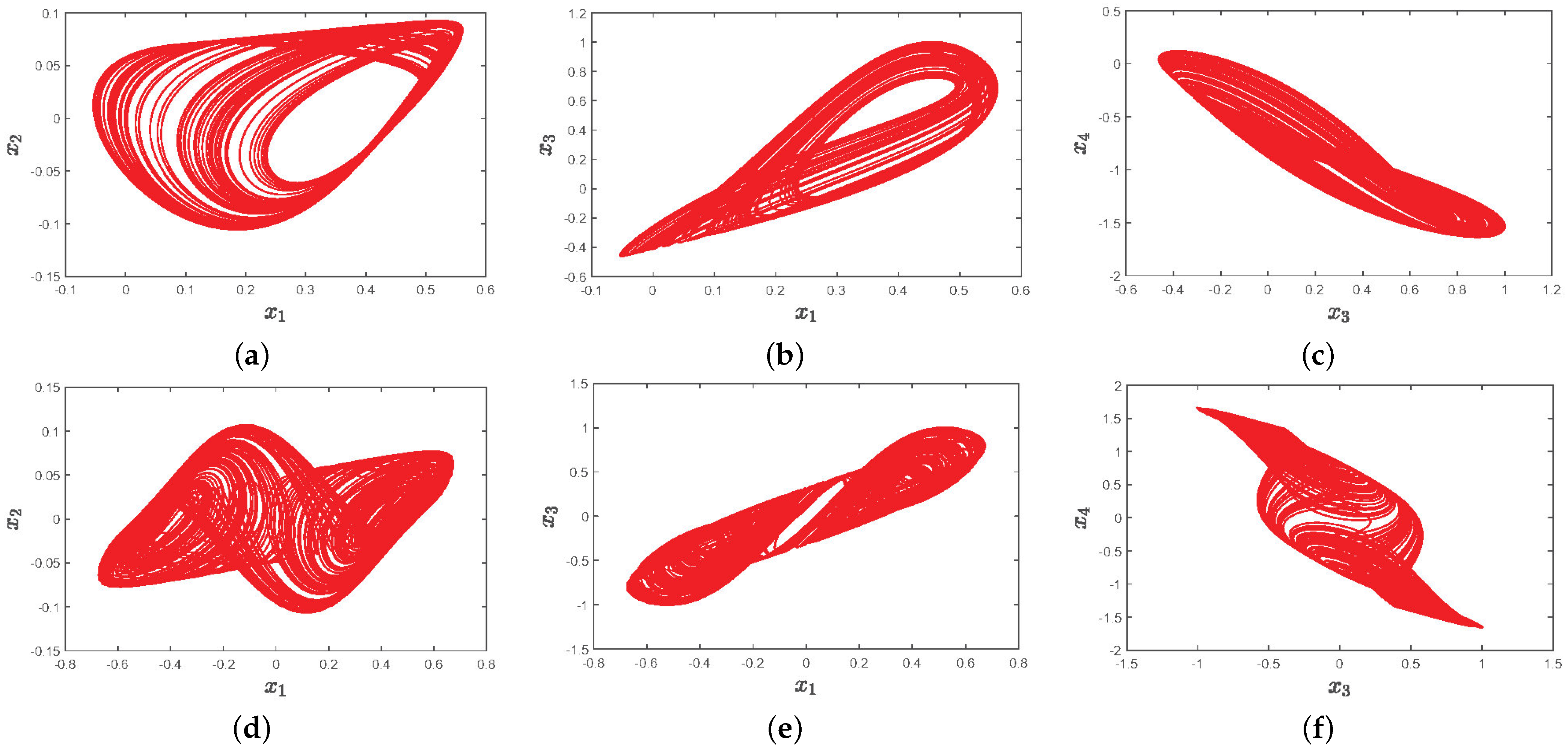
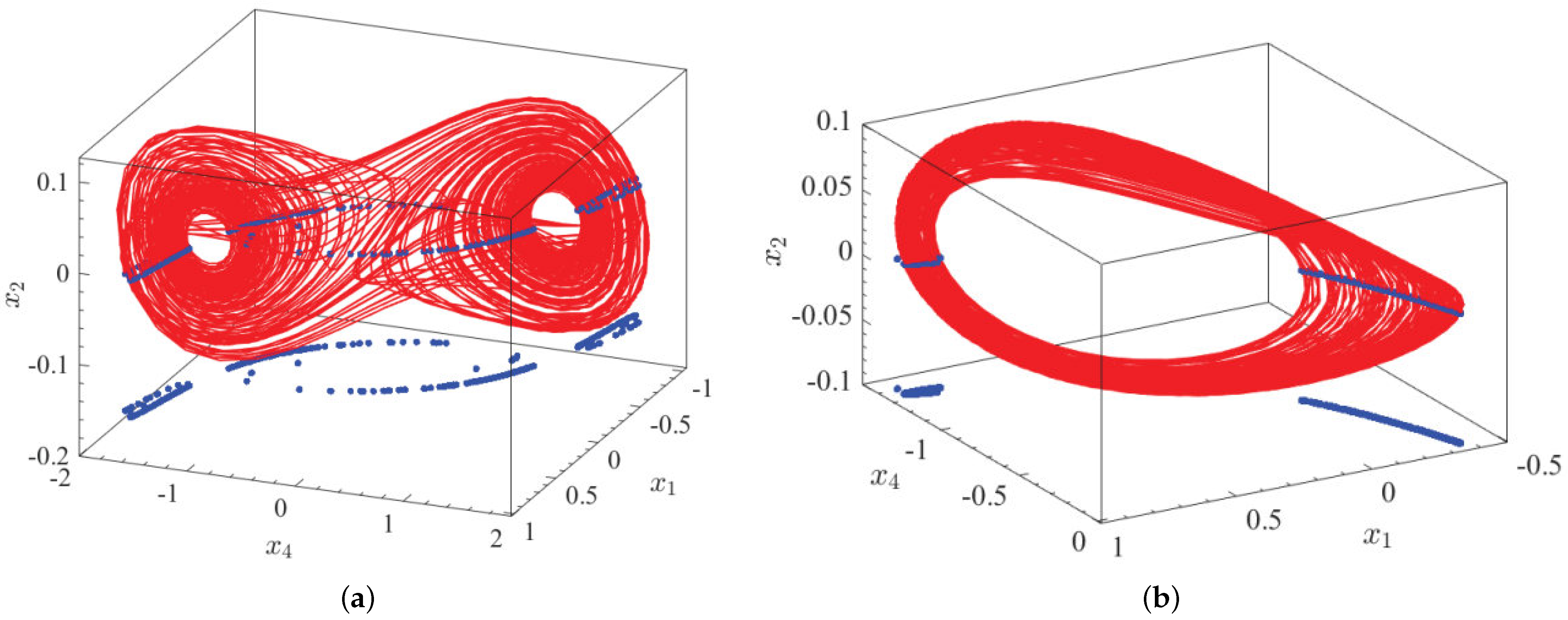
3.1. Incommensurate Aystem Phase Diagram and Poincaré Analysis

The incommensurate system parameters are set as $a=3$, $b=12$, $c=2$, $d=34$, $e=-37$, and $f=-12$ and the initial value is $x_0=\left(0.1,0.1,0.1,0.1\right)$. Furthermore, when $q_1=q_2=q_3=q_4=0.85$. Then, the phase diagram of the commensurate system can be obtained as shown in Figure 1a–c. Similarly, if the system parameters are not changed, only the fractional orders are changed $q_1=q_2=q_3=0.70$, $q_4=0.90$, and the phase diagram of the incommensurate system is shown in Figure 1d–f. By comparing the phase diagrams of the commensurate system and the incommensurate system in Figure 1, it is found that the incommensurate system obviously produces more complex chaotic attractors.

Poincaré section is composed of multiple branches, and have different branches in different directions. It can be seen that it can represent an extremely rich dynamic phase trajectory. As shown in Figure 2a,b, the cross sections at $x_2=0$ are shown, respectively, and their parameters are taken as $a=5$, $b=12$, $c=3$, $d=32$, $e=-37$, $f=-12$, $q_1=0.62$, $q_2=0.61$, $q_3=0.65$, $q_4=0.73$; $a=4$, $b=12$, $c=3$, $d=32$, $e=37$, $f=-12$, $q_1=0.60$, $q_2=0.65$, $q_3=0.60$, and $q_4=0.60$; it can be found that the Poincaré section of the incommensurate system in the three-dimensional space and its projection on the plane. It can be found that the Poincaré section projection on the plane is irregular point distribution under two sets of different parameters. This further proves that the fractional order causes the complex dynamic behavior of the incommensurate system.

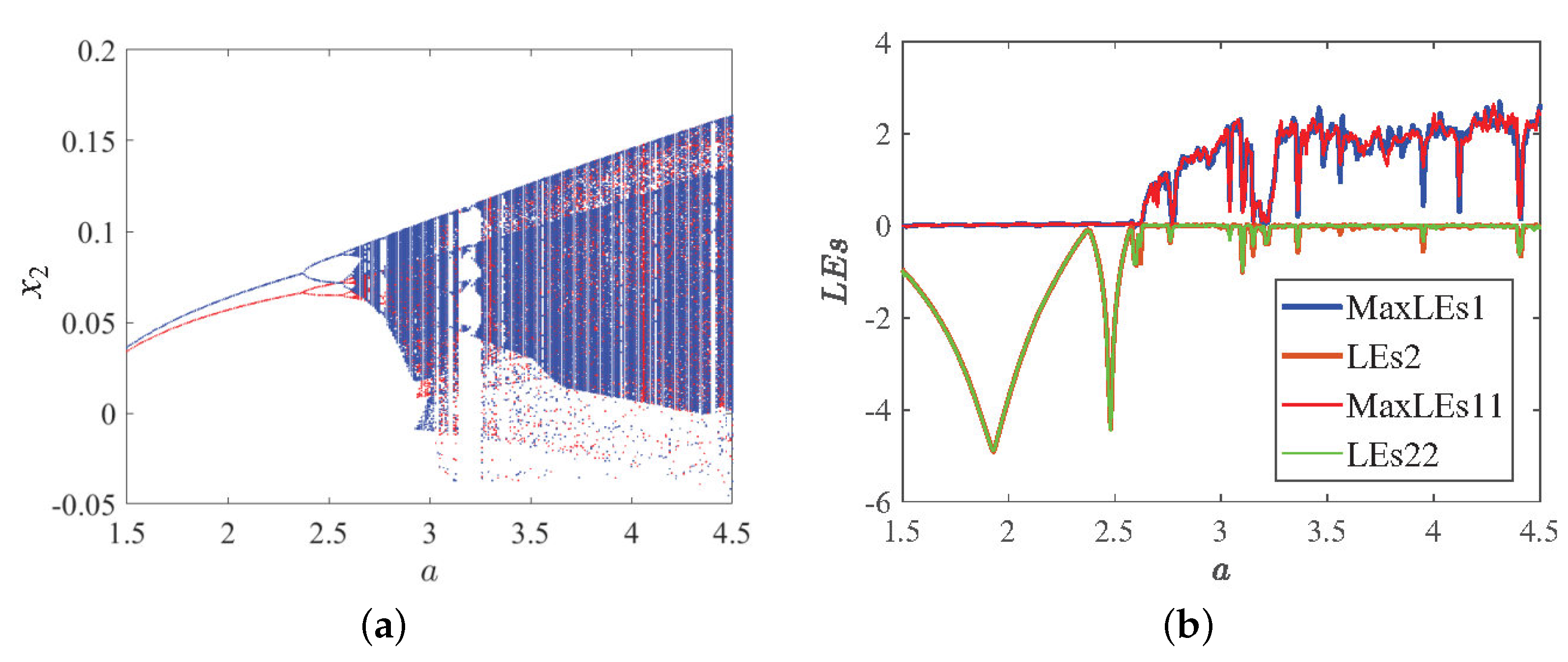
3.2. Dynamic Analysis of Fractional Orders Change in Incommensurate System

To further investigate the changes in dynamic behavior of the system under different fractional-order values, the parameters of system Equation (8) are selected as $a=3$, $b=12$, $c=2$, $d=34$, $e=-37$, and $f=-12$. The fractional orders are set within the range $q_i\in (0.8,1)$ for $i=1,2,3,4$, while $q_j=0.85$ for $j\ne i$. With these parameter settings, the bifurcation diagram and Lyapunov exponent spectrum of the incommensurate system can be obtained, as shown in Figure 3. Only the first three LEs are described here because the fourth Lyapunov exponent remains below zero and thus is not discussed.

It was found that when the fractional-order values $q_i(i=1,2,3,4)$ are inconsistent, the incommensurate system exhibits more abundant dynamic phenomena. This is primarily because different fractional orders introduce varying memory effects and dynamic responses into the system, resulting in more complex and diverse dynamical behaviors. Specifically, the inconsistency in fractional orders leads to different time scales and dynamic characteristics in the coupling and feedback mechanisms among the state variables, thereby promoting a wider range of chaotic behaviors and bifurcation patterns under the same parameter settings. Additionally, it was observed that the fractional orders $q_i(i=1,2,3,4)$ corresponding to different equations have a significant impact on the dynamic characteristics of the incommensurate system Equation (8). In particular, when the fractional order $q_2\in (0.95,1)$, its influence on the incommensurate system is most significant compared to the fractional orders $q_1$, $q_3$, and $q_4$, where variations in $q_2$ play a more prominent role in regulating system stability and chaotic properties.

3.3. Coexistence Dynamics Phenomenon of Incommensurate System Parameter Changes

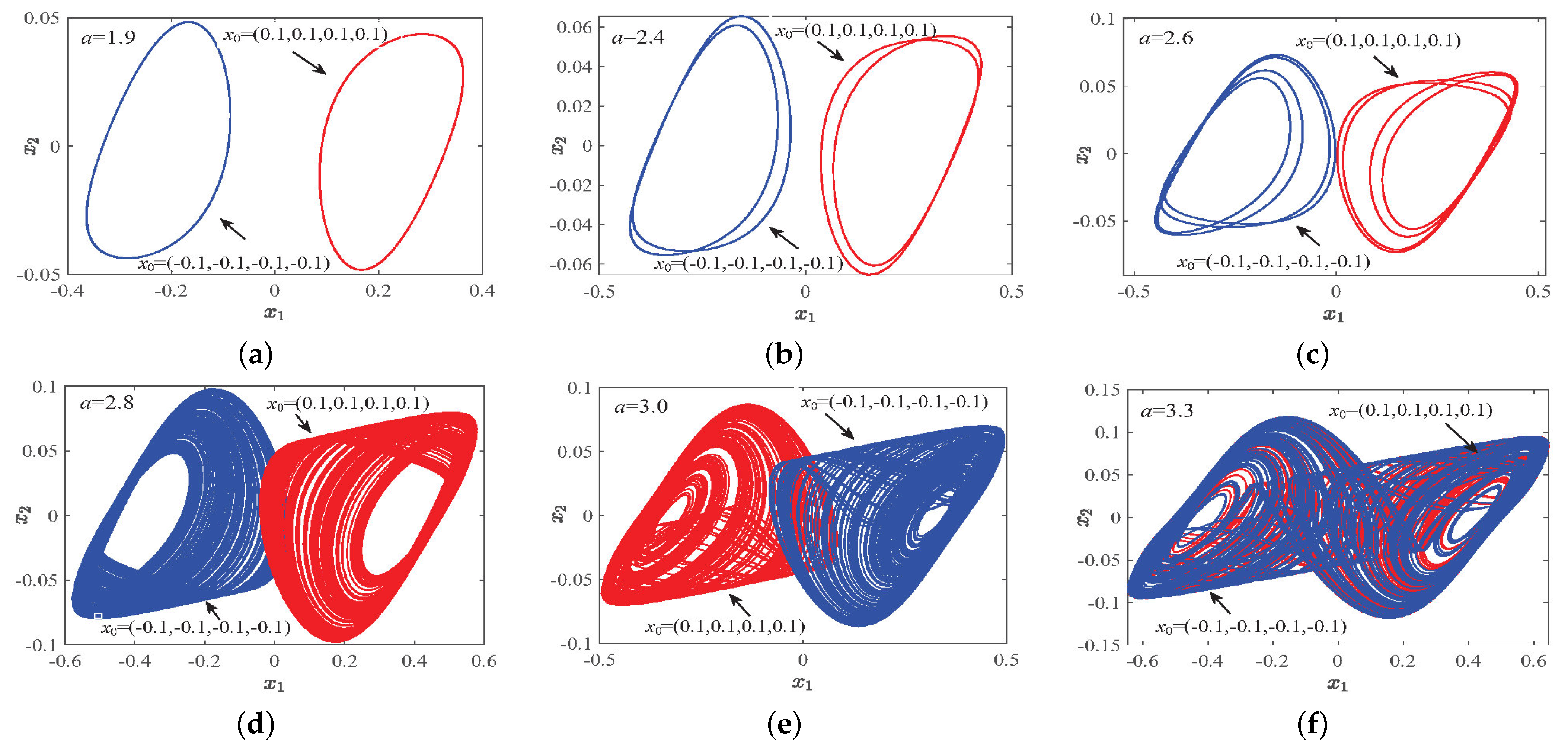
3.3.1. Dynamic Phenomena of Parameter a Change

There are many factors influencing the dynamics of memristor system, including parameters, initial values, internal parameters of memristor, internal initial values, and fractional orders. For this incommensurate memristor system, considering the change interval of the parameter $a\in (1.5,4.5)$, the coexistence bifurcation diagram of the local maximum of the incommensurate system variable $x_2$ shown in Figure 4a,b; the coexistence LEs of the incommensurate system obtained based on QR decomposition method are, respectively, drawn through the numerical simulation of the Adomian algorithm. The values of other parameters except variable parameters are $b=12$, $c=2$, $d=32$, $e=-37$, and $f=-12$, the fractional-order values are $q_1=0.75$, $q_2=0.70$, $q_3=0.75$, and $q_4=0.85$. Furthermore, the initial values of the two pairs of coexistence are $x_0=(0.1,0.1,0.1,0.1)$ and ${\widehat{x}}_0=(-0.1,-0.1,-0.1,-0.1)$. As illustrated in Figure 4a, the coexistence bifurcation diagrams under two corresponding pairs of initial conditions are represented in red (the initial value is $x_0$) and blue (the initial value is ${\widehat{x}}_0$), respectively. It is observed that under the influence of parameter a, the incommensurate system exhibits obvious period-doubling bifurcations along the bifurcation path, ultimately leading the system into a chaotic state. Moreover, as shown in Figure 4b, the coexistence Lyapunov exponents (LEs) under varying initial conditions are further described. The blue trajectory represents the maximum Lyapunov exponent with the initial value $x_0=(0.1,0.1,0.1,0.1)$, while the yellow trajectory represents the maximum Lyapunov exponent with the initial value ${\widehat{x}}_0=(-0.1,-0.1,-0.1,-0.1)$. Simultaneously, red and green trajectories are used to illustrate the second largest Lyapunov exponents under the two sets of initial values. To clearly depict the dynamic trend of the incommensurate system’s LEs, the third and fourth largest Lyapunov exponents are not further plotted, as the other two LEs remain below zero. Therefore, it can be observed in Figure 4b that the maximum Lyapunov exponent values of the blue and red curves overlap, indicating that under the two different initial conditions, the type of attractors shown in Equation (8) is the same, and the dynamic phenomena reflected by comparing the coexistence bifurcation diagram and coexistence LEs are consistent.

The study reveals that when the parameter a varies, the system undergoes a transition from stable periodic motion to period-doubling bifurcations, eventually entering a chaotic state. This period-doubling bifurcation phenomenon is a common dynamic characteristic in chaotic systems, indicating the system’s sensitivity to parameter changes. Specifically, the increase in parameter a enhances the system’s nonlinearity, thereby triggering bifurcations. Period-doubling bifurcations involve the splitting of a stable periodic orbit into two periodic orbits. When this bifurcation process repeats, the system ultimately exhibits complex chaotic behavior. This dynamic process not only validates the complexity of the system under varying parameter conditions but also provides a theoretical foundation for further research on synchronization control of incommensurate fractional-order chaotic systems.

In order to further explain the characteristic type of coexistence attractor reflected by the incommensurate system on the bifurcation path, by plotting the coexisting attractor phase diagram shown in Figure 5, it shows the coexisting attractor phase diagram with different initial values, where the blue and red tracks are at the initial values of $x_0=(0.1,0.1,0.1,0.1)$ and ${\widehat{x}}_0=(-0.1,-0.1,-0.1,-0.1)$, respectively. With the gradual increase in parameter a, it is found that there are various types of coexisting chaotic attractors, as shown in Figure 5.

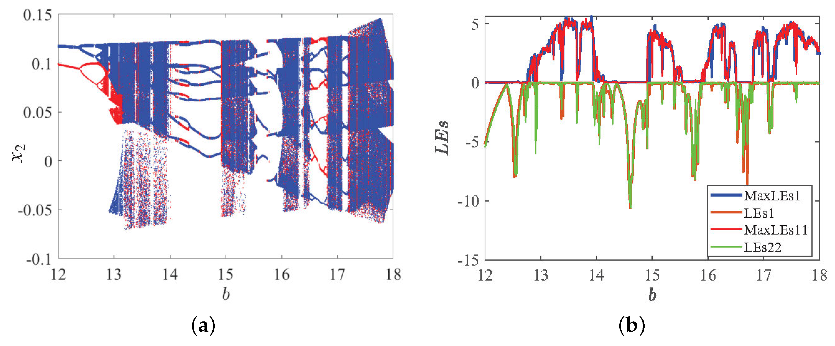
3.3.2. Dynamic Phenomena of Parameter b Change

When b is a parameter variable of incommensurate system, by setting the incommensurate system parameters $a=3$, $c=2$, $d=32$, $e=-37$, and $f=-12$ and the corresponding fractional orders are $q_1=0.61$, $q_2=0.62$, $q_3=0.52$, and $q_4=0.83$. Furthermore, the initial values are selected as $x_0=(0.1,0.1,0.1,0.1)$ and ${\widehat{x}}_0=(-0.1,-0.1,-0.1,-0.1)$. The coexistence bifurcation diagrams and LEs trajectory can be obtained as shown in Figure 6. In Figure 6a, the red track represents the initial value $x_0=(0.1,0.1,0.1,0.1)$, and the blue track represents the initial value ${\widehat{x}}_0=(-0.1,-0.1,-0.1,-0.1)$. It can be seen from Figure 6a that there are multiple period doubling bifurcations in the coexistence bifurcation diagram of parameter b changes. Further, when the period window $b=14$, it is found that the incommensurate system starts to appear the coexistence of chaotic bubbles, then when $b\in (15.4,15.8)$, a short periodic window appears. When $b>15.8$, the coexistence periodic window is entered, and when $b=16.7$, the coexistence symmetric period-2 attractor appears. Finally, after $b>16.8$, the incommensurate system is completely chaotic. In Figure 6b, the first and second LEs curves under two initial values are plotted, respectively, and it is found that they are completely consistent with the dynamic phenomena described by the coexistence bifurcation diagram. Moreover, in order to further explain the coexistence and bifurcation phenomenon in the incommensurate system, The specific type coexistence attractor phase diagram of the incommensurate system in plane $x_1-x_2$ is described in Figure 7.

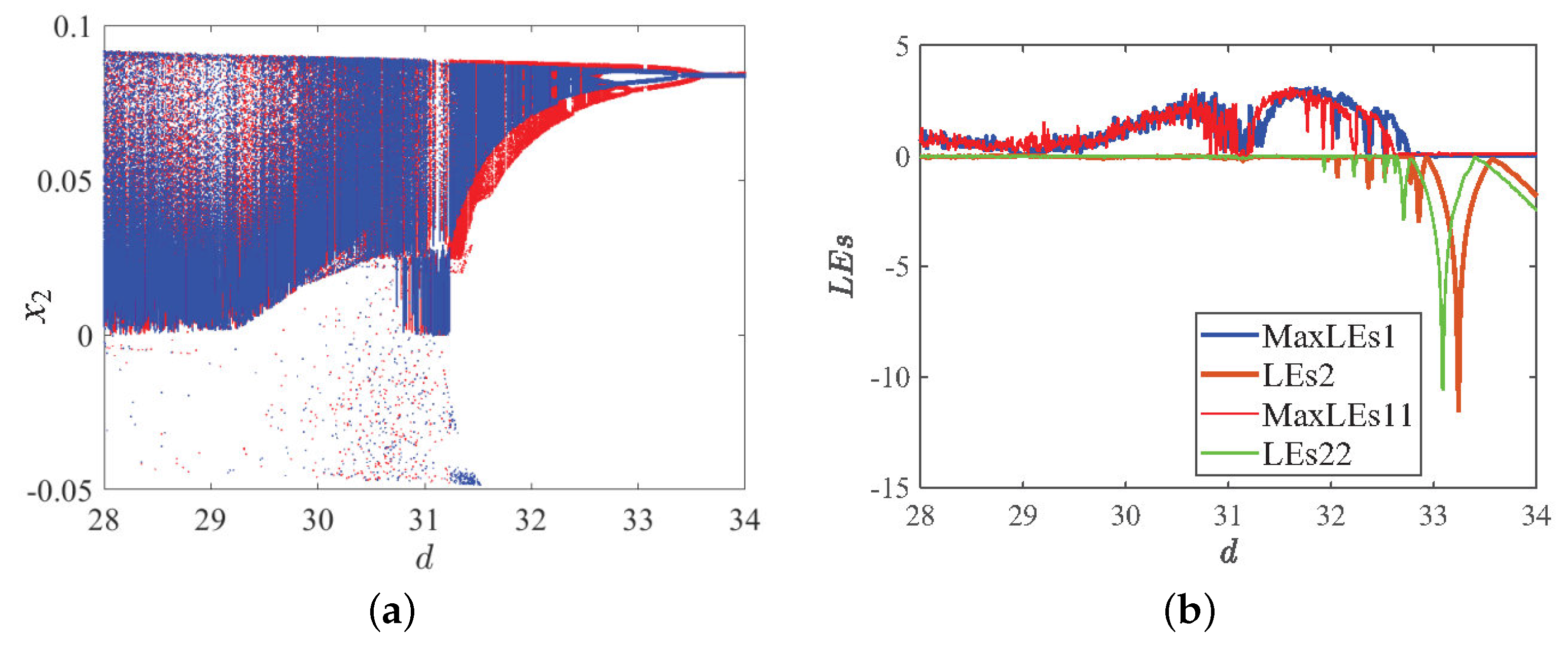
3.3.3. Dynamic Phenomena of Parameter d Change

Similarly, the incommensurate system parameter d is selected as the independent variable to study the complex dynamic behavior of the incommensurate system, other parameters are selected as $a=4$, $b=12$, $c=3$, $e=-37$, and $f=-12$. Furthermore, the fractional-order values are $q_1=0.60$, $q_2=0.65$, $q_3=0.60$, and $q_4=0.68$. Further, the values of the two pairs of initial values are $x_0=(0.1,0.1,0.1,0.1)$ and ${\widehat{x}}_0=(-0.1,-0.1,-0.1,-0.1)$. We describe the coexistence bifurcation diagram and coexistence LEs of the incommensurate system in Figure 8, where the red represents the initial value $x_0=(0.1,0.1,0.1,0.1)$ and the blue represents the initial value ${\widehat{x}}_0=(-0.1,-0.1,-0.1,-0.1)$. The coexistence bifurcation diagram of the incommensurate system is studied by changing parameter d as shown in Figure 8a, and the red represents the initial value $x_0$, meanwhile, the blue represents the initial value ${\widehat{x}}_0$. The chaotic window appears first, and then changes with the parameter d until a reverse-period doubling-bifurcation path appears, until the end, when $d=33.4$. Similarly, the coexistence LEs of the incommensurate system are further plotted and only the first two maximum LEs are taken. The values of the third and fourth LEs are always below zero, as shown in Figure 8b. The dynamic behavior consistent with the coexistence bifurcation diagram can be obtained, and the characteristic types of the incommensurate system attractor when the parameter d changes are elaborated in Figure 9a–f.

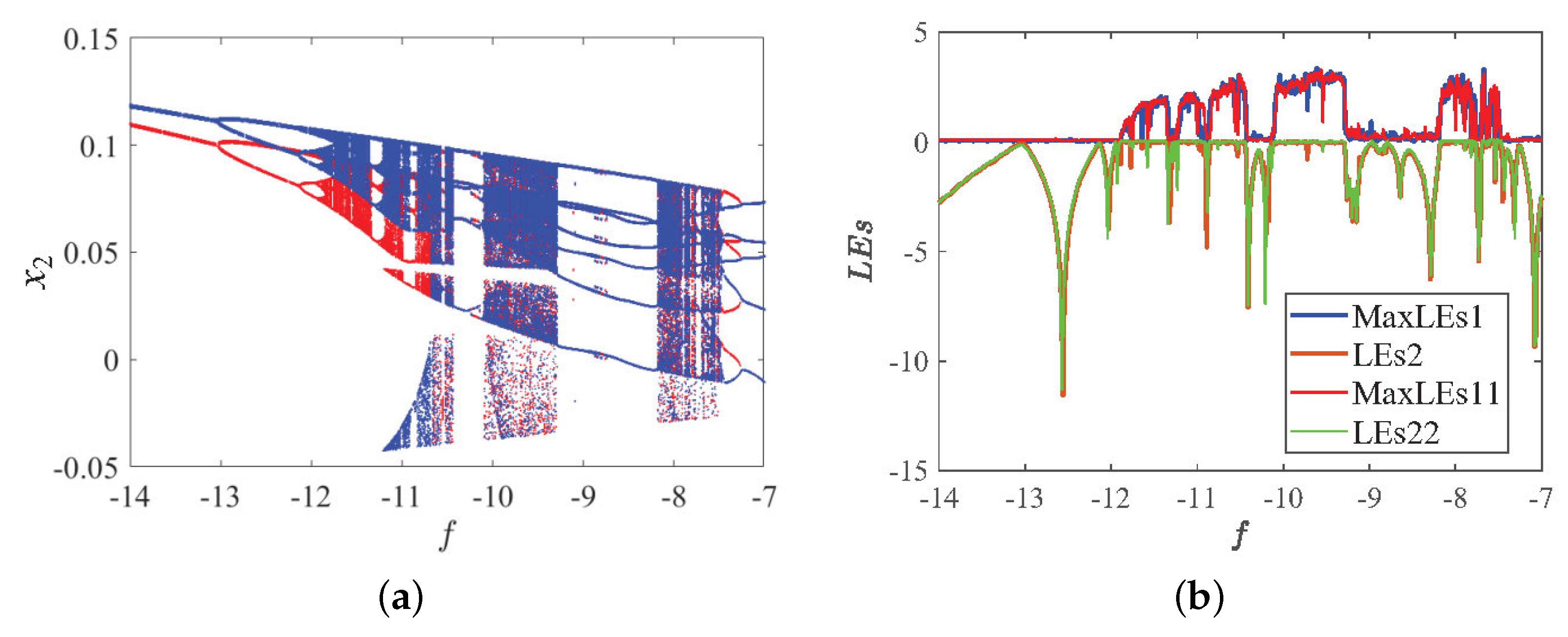
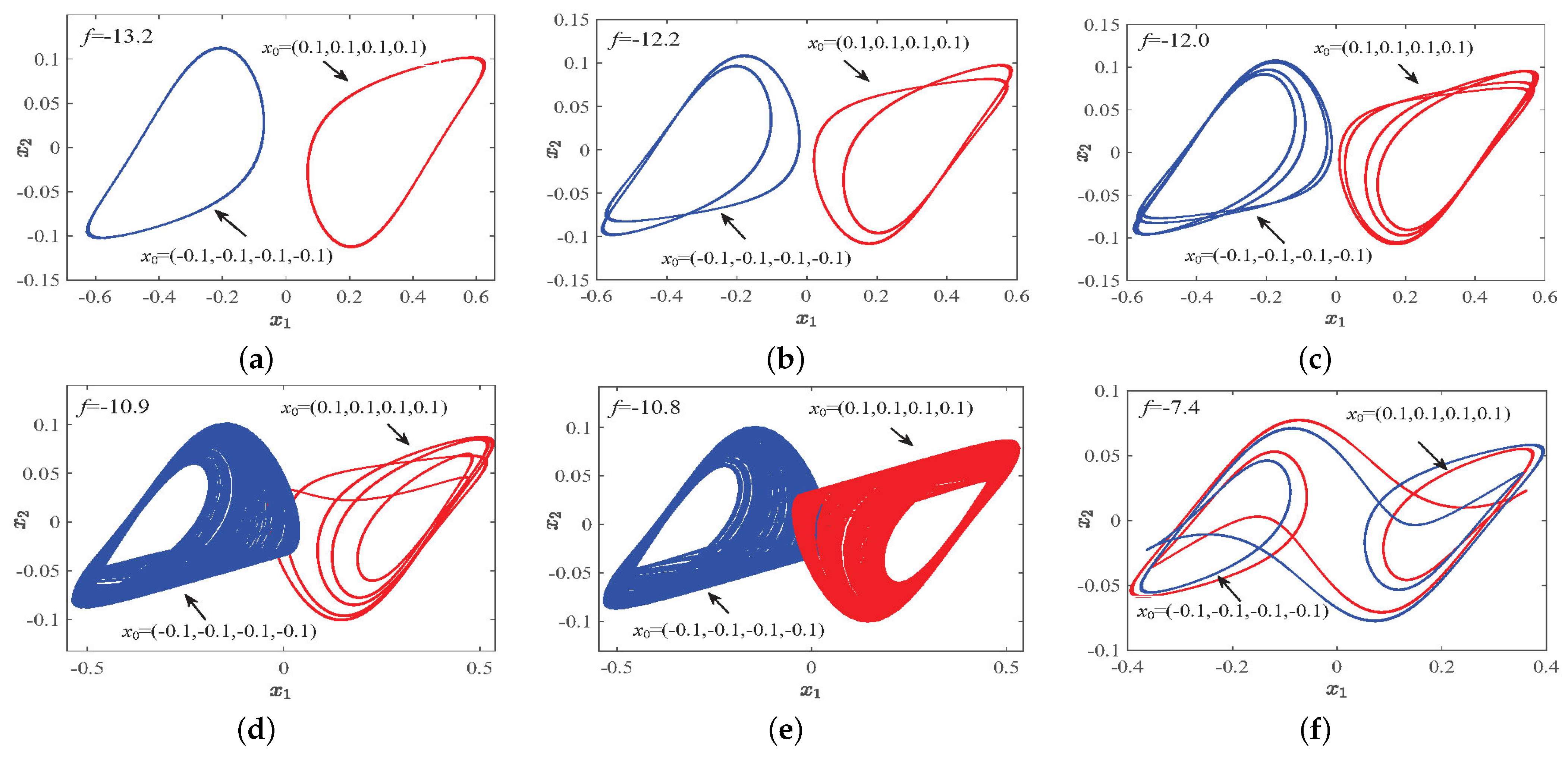
3.3.4. Dynamic Phenomena of Parameter f Change

When the study parameter is taken as the independent variable, the selection parameters are $a=4$, $b=12$, $c=3$, $d=32$, $e=-37$, $q_1=0.68$, $q_2=0.48$, $q_3=0.72$, $q_4=0.73$. Furthermore, the initial value is selected as $x_0=(0.1,0.1,0.1,0.1)$ and ${\widehat{x}}_0=(-0.1,-0.1,-0.1,-0.1)$. Figure 10 shows that, when the initial value $x_0=(0.1,0.1,0.1,0.1)$ is red, the initial value ${\widehat{x}}_0=(-0.1,-0.1,-0.1,-0.1)$ is blue. When the variable f is used as the coexistence bifurcation parameter, it is found that it enters chaotic with period doubling bifurcation, and then ends with reverse-period doubling bifurcation (Shown in Figure 10a, the red represents the initial value $x_0$, meanwhile, the blue represents the initial value ${\widehat{x}}_0$). In Figure 10b, the dynamics behavior of coexisting LEs is completely consistent with that described in the coexistence bifurcation diagram. The coexistence attractors of different types under different parameters f are plotted in the $x_1-x_2$ plane, as shown in Figure 11.

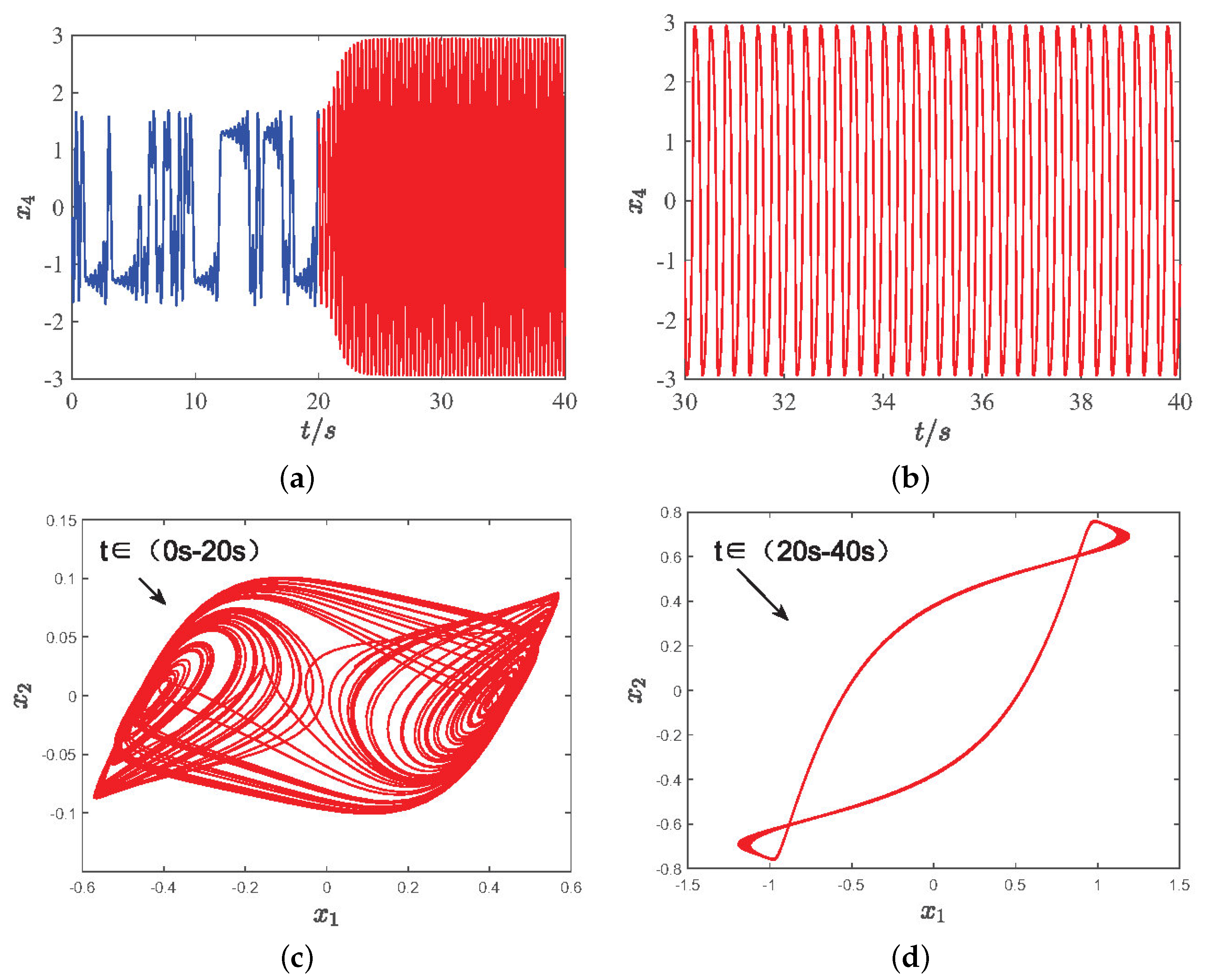
3.4. Dynamic Behavior of Chaotic Degeneration in Incommensurate Fractional-Order System

The incommensurate system is in a chaotic state within a certain time range, and then appears to sink in a periodic state, which is called chaotic degradation. In order to study the chaotic degenerate dynamics of the incommensurate system, the parameters are selected as $a=2.5$, $b=12.8$, $c=1.5$, $d=28$, $e=-37$, $f=-12$, $q_1=0.65$, $q_2=0.75$, $q_3=0.70$, and $q_4=0.64$. Furthermore, the initial value is selected as $x_0=(0.1,0.1,0.1,0.1)$. Therefore, the time–domain waveform of the incommensurate system state variable $x_4$ and the phase diagram of the incommensurate system on the $x_1-x_2$ plane in the same time period are drawn in Figure 12. In Figure 12a, it is found that chaos appears before the time period $t<$ 20 s (See the blue in Figure 12a), and degenerates to a periodic pole state after the time period $t>$ 20 s (See the red in Figure 12a); moreover, the time–domain waveform within the t me $t\in$ (30–40 s) is plotted separately, as shown in Figure 12b, the regular changes of the time–domain waveform indicate a stable periodic state. The phase diagram of the incommensurate system can also be drawn in the corresponding interval as shown in Figure 12c,d, and the results consistent with the time–domain waveform can be found, it can be further known that a double-scroll chaotic attractor appears before $t<$ 20 s, and a stable periodic limit cycle state appears after $t>$ 20 s. Therefore, it can be proved that the incommensurate fractional-order memristor system has rich chaotic degenerate behavior.

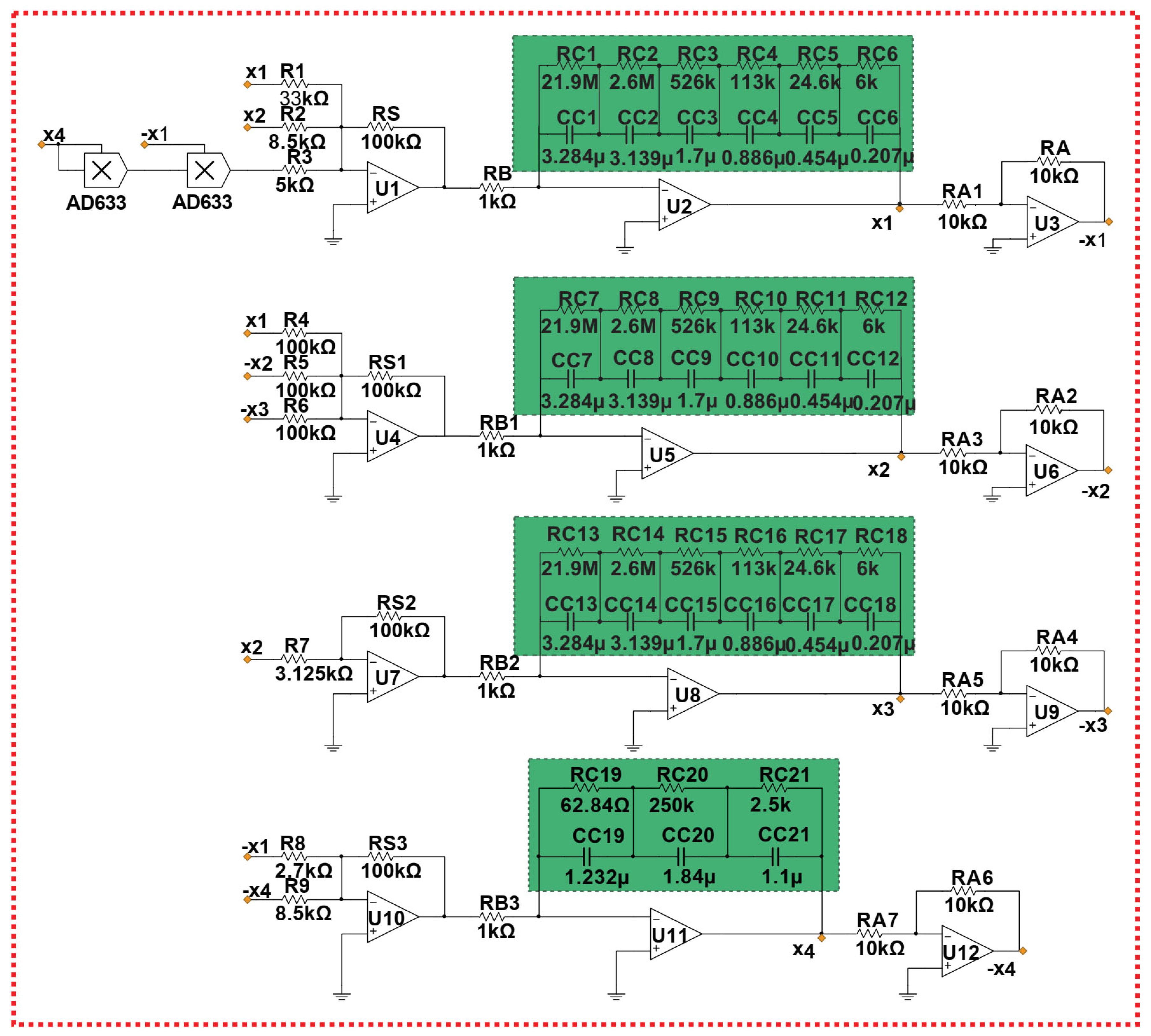
4. Analog Circuit Implementation of Incommensurate System

The chain model is widely used in the design of fractional cell circuit models. Therefore, in analog circuit experiments, the TL0812 operational amplifier and the AD633 analog multiplier, produced by Texas Instruments (Dallas, TX, USA) and Analog Devices (Wilmington, MA, USA), respectively, were chosen to implement the nonlinear functionalities of the analog circuit, with an output coefficient of 1 and a chip power supply voltage of DC ± 15 V. Based on the incommensurate fractional-order system Equation (8), the schematic diagram of the incommensurate equivalent analog circuit is designed as shown in Figure 13.

The equivalent analog circuit integrates fractional-order differentiators with various circuit components such as resistors, capacitors, and operational amplifiers to realize the dynamic relationships among the system variables as described in Equation (8). Specifically, different resistor and capacitor values correspond to the system parameters a, b, d, and f, while operational amplifiers and multipliers are utilized to implement nonlinear terms and coupling relationships. This circuit design approach ensures that the analog circuit accurately reflects the dynamic behavior of the incommensurate fractional-order system. Based on the circuit schematic and the circuit theorems of the incommensurate system, the equivalent circuit equations of the incommensurate system corresponding to system Equation (8) are obtained as follows:

$$\left\{\begin{array}{c}{\displaystyle \frac{d^{q_1}{x}_1}{dt}}={\displaystyle \frac{RS}{R_1}}{\displaystyle \frac{1}{RBC{C}_0}}{\displaystyle \frac{RA}{R{A}_1}}{x}_1+{\displaystyle \frac{RS}{R_2}}{\displaystyle \frac{1}{RBC{C}_0}}{\displaystyle \frac{RA}{R{A}_1}}{x}_2\hfill \\ +{\displaystyle \frac{RS}{R_3}}{\displaystyle \frac{1}{RBC{C}_0}}{\displaystyle \frac{RA}{R{A}_1}}{x}_4\left(-x_1\right)\hfill \\ {\displaystyle \frac{d^{q_2}{x}_2}{dt}}={\displaystyle \frac{R{S}_1}{R_4}}{\displaystyle \frac{1}{R{B}_{1}C{C}_0}}{\displaystyle \frac{R{A}_2}{R{A}_3}}{x}_1+{\displaystyle \frac{R{S}_1}{R_5}}{\displaystyle \frac{1}{R{B}_{1}C{C}_0}}{\displaystyle \frac{R{A}_2}{R{A}_3}}\left(-x_2\right)\hfill \\ +{\displaystyle \frac{R{S}_1}{R_6}}{\displaystyle \frac{1}{R{B}_{1}C{C}_0}}{\displaystyle \frac{R{A}_2}{R{A}_3}}\left(-x_3\right)\hfill \\ {\displaystyle \frac{d^{q_3}{x}_3}{dt}}={\displaystyle \frac{R{S}_2}{R_7}}{\displaystyle \frac{1}{R{B}_{2}C{C}_0}}{\displaystyle \frac{R{A}_4}{R{A}_5}}{x}_2\hfill \\ {\displaystyle \frac{d^{q_4}{x}_4}{dt}}={\displaystyle \frac{R{S}_3}{R_8}}{\displaystyle \frac{1}{R{B}_{3}C{C}_0}}{\displaystyle \frac{R{A}_6}{R{A}_7}}\left(-x_1\right)+{\displaystyle \frac{R{S}_3}{R_9}}{\displaystyle \frac{1}{R{B}_{3}C{C}_0}}{\displaystyle \frac{R{A}_4}{R{A}_5}}\left(-x_4\right)\hfill \end{array}\right.$$

(29)

Based on the above schematic diagram of the incommensurate system equivalent circuit, the phase diagrams of the $x_1-x_2$, $x_1-x_3$, and $x_3-x_4$ planes of the incommensurate system are obtained as shown in Figure 14; these are consistent with the numerical simulation results of the incommensurate system, thereby validating the accuracy of the equivalent circuit design.

5. Fixed-Time Synchronization Control of Incommensurate System

In the case of interference and parameter uncertainty, it is possible to realize synchronization control of both the leader system and the follower system within a fixed upper time limit.

Lemma 1. 

Consider the existence of fractional-order systems [43],

$$D_{t_0}^{q}f\left(x\right)=-\delta f{\left(x\right)}^{{\displaystyle \frac{\varpi }{w}}}-\phi f{\left(x\right)}^{{\displaystyle \frac{ϵ}{\epsilon }}},f\left(0\right)=f_0,q_j\in \left(0,1\right],(j=1,2,3,4)$$

(30)

where $\delta ,\phi >0$, $\varpi ,w,ϵ,\epsilon$ are positive integers, and satisfy $\varpi >w$ and $ϵ<\epsilon$; then, we can know that Equation (30) is stable within the range of fixed time, and the upper bound time function of convergence is

$$T<{\displaystyle \frac{1}{\delta }}{\displaystyle \frac{w}{\varpi -w}}+{\displaystyle \frac{1}{\phi }}{\displaystyle \frac{\epsilon }{\epsilon -ϵ}}$$

(31)

Lemma 2. 

If there are any non-negative real numbers $\left({\sigma }_1,{\sigma }_2,\cdots ,{\sigma }_N\right)$ and $0<p\le 1$, then the following inequality is established [44],

$${\sum }_{j=1}^N({\sigma }_j^p)\ge {\left({\sum }_{j=1}^N{\sigma }_j\right)}^p$$

(32)

Lemma 3. 

If there are any non-negative real numbers, then the following inequality is established [44],

$${\sum }_{j=1}^N({\sigma }_j^p)\ge N^{(1-p)}{\left({\sum }_{j=1}^N{\sigma }_j\right)}^p$$

(33)

Lemma 4. 

If the equilibrium point of the system $\dot{y}=f(t,y)$ is $y=0$, and fields with $y=0$ are included in $D\subset R^n$. Let is a continuous differentiable function; then, we can know that the following inequality is true

$$\begin{array}{c}{l}_1{\Vert y\Vert }^a\le V\left(t,y\right)\le l_2{\Vert y\Vert }^a\\ \dot{V}\left(y\right)\le -l_3{\Vert y\Vert }^a\end{array}$$

(34)

where $y\in D$, $l_1,l_2,l_3$ are positive integers, then the system shows exponential convergence at the equilibrium point $y=0$ [45].

5.1. Main Discussion

Considering that the main system of incommensurate fractional-order system is

$$\left\{\begin{array}{c}{D}_{t_0}^{q_1}{x}_1=a{x}_1+b{x}_2-c{x}_1{x_4}^2+\Delta f_1\left(x,t\right)+d_1^{f\left(t\right)}+u_1\hfill \\ D_{t_0}^{q_2}{x}_2=x_1-x_2-x_3+\Delta f_2\left(x,t\right)+d_2^{f\left(t\right)}+u_2\hfill \\ D_{t_0}^{q_3}{x}_3=d{x}_2+\Delta f_3\left(x,t\right)+d_3^{f\left(t\right)}+u_3\hfill \\ D_{t_0}^{q_4}{x}_4=e{x}_1-f{x}_4+\Delta f_4\left(x,t\right)+d_4^{f\left(t\right)}+u_4\hfill \end{array}\right.$$

(35)

where $q_j\in (0,1)\left(j=1,2,3,4\right)$ is the fractional orders of the incommensurate system, and the state variables of the main system is $x(t)={\left[x_1,x_2,x_3,x_4\right]}^T$, $u_j(j=1,2,3,4)$ represents the control input of the main system. The bounded uncertainty term and disturbance term of the main system are represented by $\Delta f_j\left(x,t\right)(j=1,2,3,4)$ and $d_j^{f\left(t\right)}(j=1,2,3,4)$, respectively.

The follower system of the same incommensurate fractional-order system is expressed as

$$\left\{\begin{array}{c}{D}_{t_0}^{q_1}{x}_{s1}=a{x}_{s1}+b{x}_{s2}-c{x}_{s1}{x_{s4}}^2+\Delta g_{s1}\left(x,t\right)+d_{s1}^{g\left(t\right)}\hfill \\ D_{t_0}^{q_2}{x}_{s2}=x_{s1}-x_{s2}-x_{s3}+\Delta g_{s2}\left(x,t\right)+d_{s2}^{g\left(t\right)}\hfill \\ D_{t_0}^{q_3}{x}_{s3}=d{x}_{s2}+\Delta g_{s3}\left(x,t\right)+d_{s3}^{g\left(t\right)}\hfill \\ D_{t_0}^{q_4}{x}_{s4}=e{x}_{s1}-f{x}_{s4}+\Delta g_{s4}\left(x,t\right)+d_{s4}^{g\left(t\right)}\hfill \end{array}\right.$$

(36)

Similarly, where $q_j\in (0,1)\left(j=1,2,3,4\right)$ is the fractional orders of the incommensurate system, the state variables of the follower system is $x(t)={\left[x_{\mathrm{s}1},x_{\mathrm{s}2},x_{s3},x_{s4}\right]}^T$; the bounded uncertainty term and disturbance term of the main system are represented by $\Delta g_{sj}\left(x,t\right)(j=1,2,3,4)$ and $d_{sj}^{g\left(t\right)}(j=1,2,3,4)$, respectively.

Let the uncertainty and disturbance terms in the leader system and follower system be bounded functions as follows:

$$\left\{\begin{array}{c}\left|\Delta f_j\left(x,t\right)\right|\le k_1\hfill \\ \left|d_j^{f\left(t\right)}\right|\le k_2\hfill \end{array}\right.(j=1,2,3,4)$$

(37)

$$\left\{\begin{array}{c}\left|\Delta g_{sj}\left(x,t\right)\right|\le k_3\hfill \\ \left|d_{sj}^{g\left(t\right)}\right|\le k_4\hfill \end{array}\right.(j=1,2,3,4)$$

(38)

where are $k_1$, $k_2$, $k_3$, $k_4$ positive bounded constants.

The synchronization error is further defined as follows:

$$\left\{\begin{array}{c}{e}_1=x_{s1}-x_1\\ e_2=x_{s2}-x_2\\ e_3=x_{s3}-x_3\\ e_4=x_{s4}-x_4\end{array}\right.$$

(39)

The derivative of order $q_j(j=1,2,3,4)$ or the time t of $D_{t_0}^{q_j}(j=1,2,3,4)$ at both ends of $e_j(j=1,2,3,4)$ is given below.

$$\left\{\begin{array}{c}{D}_{t_0}^{q_1}{e}_1=D_{t_0}^{q_1}{x}_{s1}-D_{t_0}^{q_1}{x}_1\\ D_{t_0}^{q_2}{e}_2=D_{t_0}^{q_2}{x}_{s2}-D_{t_0}^{q_2}{x}_2\\ D_{t_0}^{q_3}{e}_3=D_{t_0}^{q_3}{x}_{s3}-D_{t_0}^{q_3}{x}_3\\ D_{t_0}^{q_4}{e}_4=D_{t_0}^{q_4}{x}_{s4}-D_{t_0}^{q_4}{x}_4\end{array}\right.$$

(40)

By substituting Equations (35) and (36) into Equation (40), we can obtain the following

$$\left\{\begin{array}{c}{D}_{t_0}^{q_1}{e}_1=a{x}_{s1}+b{x}_{s2}-c{x}_{s1}{x_{s4}}^2+\Delta g_{s1}\left(x,t\right)+d_{s1}^{g\left(t\right)}\hfill \\ -\left(a{x}_1+b{x}_2-c{x}_1{x_4}^2+\Delta f_1\left(x,t\right)+d_1^{f\left(t\right)}+u_1\right)\hfill \\ D_{t_0}^{q_2}{e}_2=x_{s1}-x_{s2}-x_{s3}+\Delta g_{s2}\left(x,t\right)+d_{s2}^{g\left(t\right)}\hfill \\ =-\left(x_1-x_2-x_3+\Delta f_2\left(x,t\right)+d_2^{f\left(t\right)}+u_2\right)\hfill \\ D_{t_0}^{q_3}{e}_3=d{x}_{s2}+\Delta g_{s3}\left(x,t\right)+d_{s3}^{g\left(t\right)}\hfill \\ -\left(d{x}_2+\Delta f_3\left(x,t\right)+d_3^{f\left(t\right)}+u_3\right)\hfill \\ D_{t_0}^{q_4}{e}_4=e{x}_{s1}-f{x}_{s4}+\Delta g_{s4}\left(x,t\right)+d_{s4}^{g\left(t\right)}\hfill \\ -\left(e{x}_1-f{x}_4+\Delta f_4\left(x,t\right)+d_4^{f\left(t\right)}+u_4\right)\hfill \end{array}\right.$$

(41)

Consider the sliding surface function corresponding to the design system as follows:

$$\left\{\begin{array}{c}{s}_1=e_1+D_{t_0}^{-q_1}\left({\sigma }_1{\left|e_1\right|}^{{\displaystyle \frac{{\upsilon }_1}{{\vartheta }_1}}}\mathrm{sign}\left(e_1\right)+{\eta }_1{\left|e_1\right|}^{{\displaystyle \frac{{\varsigma }_1}{{\zeta }_1}}}\mathrm{sign}\left(e_1\right)\right)\\ s_2=e_2+D_{t_0}^{-q_2}\left({\sigma }_1{\left|e_2\right|}^{{\displaystyle \frac{{\upsilon }_1}{{\vartheta }_1}}}\mathrm{sign}\left(e_2\right)+{\eta }_1{\left|e_2\right|}^{{\displaystyle \frac{{\varsigma }_1}{{\zeta }_1}}}\mathrm{sign}\left(e_2\right)\right)\\ s_3=e_3+D_{t_0}^{-q_3}\left({\sigma }_1{\left|e_3\right|}^{{\displaystyle \frac{{\upsilon }_1}{{\vartheta }_1}}}\mathrm{sign}\left(e_3\right)+{\eta }_1{\left|e_3\right|}^{{\displaystyle \frac{{\varsigma }_1}{{\zeta }_1}}}\mathrm{sign}\left(e_3\right)\right)\\ s_4=e_4+D_{t_0}^{-q_4}\left({\sigma }_1{\left|e_4\right|}^{{\displaystyle \frac{{\upsilon }_1}{{\vartheta }_1}}}\mathrm{sign}\left(e_4\right)+{\eta }_1{\left|e_4\right|}^{{\displaystyle \frac{{\varsigma }_1}{{\zeta }_1}}}\mathrm{sign}\left(e_4\right)\right)\end{array}\right.$$

(42)

Here, ${\sigma }_1$, ${\eta }_1$, ${\upsilon }_1$, ${\vartheta }_1$, ${\varsigma }_1$, ${\zeta }_1$ are positive integers, and ${\upsilon }_1>{\vartheta }_1$, ${\varsigma }_1<{\zeta }_1$.

Theorem 1. 

If Equation (41) contains uncertainty and unknown external interference term, and it satisfies the conditions of bounded condition Equations (37) and (38), the following control scheme can be designed:

$$\left\{\begin{array}{c}{u}_1=-\left(a{x}_{s1}+b{x}_{s2}-c{x}_{s1}{x_{s4}}^2+\Delta g_{s1}\left(x,t\right)+d_{s1}^{g\left(t\right)}\right)\hfill \\ +\left(a{x}_1+b{x}_2-c{x}_1{x_4}^2+\Delta f_1\left(x,t\right)+d_1^{f\left(t\right)}\right)\hfill \\ -\left({\sigma }_1{\left|e_1\right|}^{{\displaystyle \frac{{\upsilon }_1}{{\vartheta }_1}}}\mathrm{sign}\left(e_1\right)+{\eta }_1{\left|e_1\right|}^{{\displaystyle \frac{{\varsigma }_1}{{\zeta }_1}}}\mathrm{sign}\left(e_1\right)\right)+{\sigma }_2{\left|s_1\right|}^{{\displaystyle \frac{{\upsilon }_2}{{\vartheta }_2}}}\mathrm{sign}\left(s_1\right)+{\eta }_2{\left|s_1\right|}^{{\displaystyle \frac{{\varsigma }_2}{{\zeta }_2}}}\mathrm{sign}\left(s_1\right)\hfill \\ u_2=x_{s1}-x_{s2}-x_{s3}+\Delta g_{s2}\left(x,t\right)+d_{s2}^{g\left(t\right)}-\left(x_1-x_2-x_3+\Delta f_2\left(x,t\right)+d_2^{f\left(t\right)}+u_2\right)\hfill \\ -\left({\sigma }_1{\left|e_2\right|}^{{\displaystyle \frac{{\upsilon }_1}{{\vartheta }_1}}}\mathrm{sign}\left(e_2\right)+{\eta }_1{\left|e_2\right|}^{{\displaystyle \frac{{\varsigma }_1}{{\zeta }_1}}}\mathrm{sign}\left(e_2\right)\right)+{\sigma }_2{\left|s_3\right|}^{{\displaystyle \frac{{\upsilon }_2}{{\vartheta }_2}}}\mathrm{sign}\left(s_3\right)+{\eta }_2{\left|s_3\right|}^{{\displaystyle \frac{{\varsigma }_2}{{\zeta }_2}}}\mathrm{sign}\left(s_3\right)\hfill \\ u_3=d{x}_{s2}+\Delta g_{s3}\left(x,t\right)+d_{s3}^{g\left(t\right)}-\left(d{x}_2+\Delta f_3\left(x,t\right)+d_3^{f\left(t\right)}+u_3\right)\hfill \\ -\left({\sigma }_1{\left|e_3\right|}^{{\displaystyle \frac{{\upsilon }_1}{{\vartheta }_1}}}\mathrm{sign}\left(e_3\right)+{\eta }_1{\left|e_3\right|}^{{\displaystyle \frac{{\varsigma }_1}{{\zeta }_1}}}\mathrm{sign}\left(e_3\right)\right)+{\sigma }_2{\left|s_3\right|}^{{\displaystyle \frac{{\upsilon }_2}{{\vartheta }_2}}}\mathrm{sign}\left(s_3\right)+{\eta }_2{\left|s_3\right|}^{{\displaystyle \frac{{\varsigma }_2}{{\zeta }_2}}}\mathrm{sign}\left(s_3\right)\hfill \\ u_4=e{x}_{s1}-f{x}_{s4}+\Delta g_{s4}\left(x,t\right)+d_{s4}^{g\left(t\right)}-\left(e{x}_1-f{x}_4+\Delta f_4\left(x,t\right)+d_4^{f\left(t\right)}+u_4\right)\hfill \\ -\left({\sigma }_1{\left|e_4\right|}^{{\displaystyle \frac{{\upsilon }_1}{{\vartheta }_1}}}\mathrm{sign}\left(e_4\right)+{\eta }_1{\left|e_4\right|}^{{\displaystyle \frac{{\varsigma }_1}{{\zeta }_1}}}\mathrm{sign}\left(e_4\right)\right)+{\sigma }_2{\left|s_4\right|}^{{\displaystyle \frac{{\upsilon }_2}{{\vartheta }_2}}}\mathrm{sign}\left(s_4\right)+{\eta }_2{\left|s_4\right|}^{{\displaystyle \frac{{\varsigma }_2}{{\zeta }_2}}}\mathrm{sign}\left(s_4\right)\hfill \end{array}\right.$$

(43)

In which ${\sigma }_2$, ${\eta }_2$, ${\upsilon }_2$, ${\vartheta }_2$, ${\varsigma }_2$, ${\zeta }_2$ are positive integers, and ${\upsilon }_2>{\vartheta }_2$, ${\varsigma }_2<{\zeta }_2$. Then, the incommensurate system can converge to the sliding mode surface in the given time $T_t$, and the upper bound function of the convergence time is shown in Equation (44) below.

$$T_t<{\displaystyle \frac{1}{{\sigma }_2{n}^{1-\frac{{\rho }_2}{{\theta }_2}}}}{\displaystyle \frac{{\vartheta }_2}{{\nu }_2-{\vartheta }_2}}+{\displaystyle \frac{1}{{\eta }_2}}{\displaystyle \frac{{\zeta }_2}{{\zeta }_2-{\varsigma }_2}}$$

(44)

Proof. 

In order to ensure that the incommensurate system converges to the sliding surface in a fixed time, the Lyapunov function is selected as

$$V_1=\left|s_1\right|+\left|s_2\right|+\left|s_3\right|+\left|s_4\right|$$

(45)

Further, the derivative of order $q_j(j=1,2,3,4)$ of time is obtained from both sides of the function of Equation (45).

$$\begin{array}{c}{D}_{t_0}^{q_j}{V}_1=\mathrm{sign}\left(s_1\right)D_{t_0}^{q_1}{s}_1+\mathrm{sign}\left(s_2\right)D_{t_0}^{q_2}{s}_2\hfill \\ +\mathrm{sign}\left(s_3\right)D_{t_0}^{q_3}{s}_3+\mathrm{sign}\left(s_4\right)D_{t_0}^{q_4}{s}_4\hfill \end{array}$$

(46)

Substituting the equation of sliding surface function Equation (42) into Equation (46), we can obtain

$$\left\{\begin{array}{c}{D}_{t_0}^{q_j}{V}_1=\left(\mathrm{sign}\left(s_1\right)\right.\left(D_{t_0}^{q_1}{e}_1+\left({\sigma }_1{\left|e_1\right|}^{{\displaystyle \frac{{\upsilon }_1}{{\vartheta }_1}}}\mathrm{sign}\left(e_1\right)+{\eta }_1{\left|e_1\right|}^{{\displaystyle \frac{{\varsigma }_1}{{\zeta }_1}}}\mathrm{sign}\left(e_1\right)\right)\right)\hfill \\ +\left(\mathrm{sign}\left(s_2\right)\right.\left(D_{t_0}^{q_2}{e}_2+\left({\sigma }_1{\left|e_2\right|}^{{\displaystyle \frac{{\upsilon }_1}{{\vartheta }_1}}}\mathrm{sign}\left(e_2\right)+{\eta }_1{\left|e_2\right|}^{{\displaystyle \frac{{\varsigma }_1}{{\zeta }_1}}}\mathrm{sign}\left(e_2\right)\right)\right)\hfill \\ +\left(\mathrm{sign}\left(s_3\right)\right.\left(D_{t_0}^{q_3}{e}_3+\left({\sigma }_1{\left|e_3\right|}^{{\displaystyle \frac{{\upsilon }_1}{{\vartheta }_1}}}\mathrm{sign}\left(e_3\right)+{\eta }_1{\left|e_3\right|}^{{\displaystyle \frac{{\varsigma }_1}{{\zeta }_1}}}\mathrm{sign}\left(e_3\right)\right)\right)\hfill \\ +\left(\mathrm{sign}\left(s_4\right)\right.\left(D_{t_0}^{q_4}{e}_4+\left({\sigma }_1{\left|e_4\right|}^{{\displaystyle \frac{{\upsilon }_1}{{\vartheta }_1}}}\mathrm{sign}\left(e_4\right)+{\eta }_1{\left|e_2\right|}^{{\displaystyle \frac{{\varsigma }_1}{{\zeta }_1}}}\mathrm{sign}\left(e_4\right)\right)\right)\hfill \end{array}\right.$$

(47)

Here, $j=1,2,3,4$.

Further, by substituting the error definition Equation (41) into Equation (47), we can obtain the following:

$$\left\{\begin{array}{c}{D}_{t_0}^{q_j}{V}_1=\left(\mathrm{sign}\left(s_1\right)\right)\left(\begin{array}{c}a{x}_{s1}+b{x}_{s2}-c{x}_{s1}{x_{s4}}^2+\Delta g_{s1}\left(x,t\right)+d_{s1}^{g\left(t\right)}\hfill \\ -\left(a{x}_1+b{x}_2-c{x}_1{x_4}^2+\Delta f_1\left(x,t\right)+d_1^{f\left(t\right)}+u_1\right)\hfill \\ +\left({\sigma }_1{\left|e_1\right|}^{{\displaystyle \frac{{\upsilon }_1}{{\vartheta }_1}}}\mathrm{sign}\left(e_1\right)+{\eta }_1{\left|e_1\right|}^{{\displaystyle \frac{{\varsigma }_1}{{\zeta }_1}}}\mathrm{sign}\left(e_1\right)\right)\hfill \end{array}\right)\hfill \\ +\left(\mathrm{sign}\left(s_2\right)\right)\left(\begin{array}{c}{x}_{s1}-x_{s2}-x_{s3}+\Delta g_{s2}\left(x,t\right)+d_{s2}^{g\left(t\right)}\hfill \\ -\left(x_1-x_2-x_3+\Delta f_2\left(x,t\right)+d_2^{f\left(t\right)}+u_2\right)\hfill \\ +\left({\sigma }_1{\left|e_2\right|}^{{\displaystyle \frac{{\upsilon }_1}{{\vartheta }_1}}}\mathrm{sign}\left(e_2\right)+{\eta }_1{\left|e_2\right|}^{{\displaystyle \frac{{\varsigma }_1}{{\zeta }_1}}}\mathrm{sign}\left(e_2\right)\right)\hfill \end{array}\right)\hfill \\ +\left(\mathrm{sign}\left(s_3\right)\right)\left(\begin{array}{c}d{x}_{s2}+\Delta g_{s3}\left(x,t\right)+d_{s3}^{g\left(t\right)}\hfill \\ -\left(d{x}_2+\Delta f_3\left(x,t\right)+d_3^{f\left(t\right)}+u_3\right)\hfill \\ +\left({\sigma }_1{\left|e_3\right|}^{{\displaystyle \frac{{\upsilon }_1}{{\vartheta }_1}}}\mathrm{sign}\left(e_3\right)+{\eta }_1{\left|e_3\right|}^{{\displaystyle \frac{{\varsigma }_1}{{\zeta }_1}}}\mathrm{sign}\left(e_3\right)\right)\hfill \end{array}\right)\hfill \\ +\left(\mathrm{sign}\left(s_4\right)\right)\left(\begin{array}{c}e{x}_{s1}-f{x}_{s4}+\Delta g_{s4}\left(x,t\right)+d_{s4}^{g\left(t\right)}\hfill \\ -\left(e{x}_1-f{x}_4+\Delta f_4\left(x,t\right)+d_4^{f\left(t\right)}+u_4\right)\hfill \\ +\left({\sigma }_1{\left|e_4\right|}^{{\displaystyle \frac{{\upsilon }_1}{{\vartheta }_1}}}\mathrm{sign}\left(e_4\right)+{\eta }_1{\left|e_4\right|}^{{\displaystyle \frac{{\varsigma }_1}{{\zeta }_1}}}\mathrm{sign}\left(e_4\right)\right)\hfill \end{array}\right)\hfill \end{array}\right.$$

(48)

In which $j=1,2,3,4$.

Next, substitute the control input Equation (43) of the incommensurate system into Equation (48) to obtain

$$\left\{\begin{array}{c}{D}_{t_0}^{q_j}{V}_1=\mathrm{sign}\left(s_1\right)\left(\begin{array}{c}-{\sigma }_2{\left|s_1\right|}^{{\displaystyle \frac{{\upsilon }_2}{{\vartheta }_2}}}\mathrm{sign}\left(s_1\right)-\Delta f_1\left(x,t\right)+\Delta g_{s1}\left(x,t\right)\hfill \\ -{\eta }_2{\left|s_1\right|}^{{\displaystyle \frac{{\varsigma }_2}{{\zeta }_2}}}\mathrm{sign}\left(s_1\right)+d_{s1}^g\left(t\right)-d_1^f\left(t\right)\hfill \end{array}\right)\hfill \\ +\mathrm{sign}\left(s_2\right)\left(\begin{array}{c}-{\sigma }_2{\left|s_2\right|}^{{\displaystyle \frac{{\upsilon }_2}{{\vartheta }_2}}}\mathrm{sign}\left(s_2\right)-\Delta f_2\left(x,t\right)+\Delta g_{s2}\left(x,t\right)\hfill \\ -{\eta }_2{\left|s_2\right|}^{{\displaystyle \frac{{\varsigma }_2}{{\zeta }_2}}}\mathrm{sign}\left(s_2\right)+d_{s2}^g\left(t\right)-d_2^f\left(t\right)\hfill \end{array}\right)\hfill \\ +\mathrm{sign}\left(s_3\right)\left(\begin{array}{c}-{\sigma }_2{\left|s_3\right|}^{{\displaystyle \frac{{\upsilon }_2}{{\vartheta }_2}}}\mathrm{sign}\left(s_3\right)-\Delta f_3\left(x,t\right)+\Delta g_{s3}\left(x,t\right)\hfill \\ -{\eta }_2{\left|s_3\right|}^{{\displaystyle \frac{{\varsigma }_2}{{\zeta }_2}}}\mathrm{sign}\left(s_3\right)+d_{s3}^g\left(t\right)-d_3^f\left(t\right)\hfill \end{array}\right)\hfill \\ +\mathrm{sign}\left(s_4\right)\left(\begin{array}{c}-{\sigma }_2{\left|s_4\right|}^{{\displaystyle \frac{{\upsilon }_2}{{\vartheta }_2}}}\mathrm{sign}\left(s_4\right)-\Delta f_4\left(x,t\right)+\Delta g_{s4}\left(x,t\right)\hfill \\ -{\eta }_2{\left|s_4\right|}^{{\displaystyle \frac{{\varsigma }_2}{{\zeta }_2}}}\mathrm{sign}\left(s_4\right)+d_{s4}^g\left(t\right)-d_4^f\left(t\right)\hfill \end{array}\right)\hfill \\ =-{\sigma }_2{\left|s_1\right|}^{{\displaystyle \frac{{\upsilon }_2}{{\vartheta }_2}}}-{\eta }_2{\left|s_1\right|}^{{\displaystyle \frac{{\varsigma }_2}{{\zeta }_2}}}-\left|\Delta f_1\left(x,t\right)\right|+\left|\Delta g_{s1}\left(x,t\right)\right|+\left|d_{s1}^g\left(t\right)\right|-\left|d_1^f\left(t\right)\right|\hfill \\ -{\sigma }_2{\left|s_2\right|}^{{\displaystyle \frac{{\upsilon }_2}{{\vartheta }_2}}}-{\eta }_2{\left|s_2\right|}^{{\displaystyle \frac{{\varsigma }_2}{{\zeta }_2}}}-\left|\Delta f_2\left(x,t\right)\right|+\left|\Delta g_{s2}\left(x,t\right)\right|+\left|d_{s2}^g\left(t\right)\right|-\left|d_2^f\left(t\right)\right|\hfill \\ -{\sigma }_2{\left|s_3\right|}^{{\displaystyle \frac{{\upsilon }_2}{{\vartheta }_2}}}-{\eta }_2{\left|s_3\right|}^{{\displaystyle \frac{{\varsigma }_2}{{\zeta }_2}}}-\left|\Delta f_3\left(x,t\right)\right|+\left|\Delta g_{s3}\left(x,t\right)\right|+\left|d_{s3}^g\left(t\right)\right|-\left|d_3^f\left(t\right)\right|\hfill \\ -{\sigma }_2{\left|s_4\right|}^{{\displaystyle \frac{{\upsilon }_2}{{\vartheta }_2}}}-{\eta }_2{\left|s_4\right|}^{{\displaystyle \frac{{\varsigma }_2}{{\zeta }_2}}}-\left|\Delta f_4\left(x,t\right)\right|+\left|\Delta g_{s4}\left(x,t\right)\right|+\left|d_{s4}^g\left(t\right)\right|-\left|d_4^f\left(t\right)\right|\hfill \\ =-{\sigma }_2{\left|s_1\right|}^{{\displaystyle \frac{{\upsilon }_2}{{\vartheta }_2}}}-{\eta }_2{\left|s_1\right|}^{{\displaystyle \frac{{\varsigma }_2}{{\zeta }_2}}}-\left[\left|\Delta f_1\left(x,t\right)\right|-\left|\Delta g_{s1}\left(x,t\right)\right|-\left|d_{s1}^g\left(t\right)\right|+\left|d_1^f\left(t\right)\right|\right]\hfill \\ -{\sigma }_2{\left|s_2\right|}^{{\displaystyle \frac{{\upsilon }_2}{{\vartheta }_2}}}-{\eta }_2{\left|s_2\right|}^{{\displaystyle \frac{{\varsigma }_2}{{\zeta }_2}}}-\left[\left|\Delta f_2\left(x,t\right)\right|-\left|\Delta g_{s2}\left(x,t\right)\right|-\left|d_{s2}^g\left(t\right)\right|+\left|d_2^f\left(t\right)\right|\right]\hfill \\ -{\sigma }_2{\left|s_3\right|}^{{\displaystyle \frac{{\upsilon }_2}{{\vartheta }_2}}}-{\eta }_2{\left|s_3\right|}^{{\displaystyle \frac{{\varsigma }_2}{{\zeta }_2}}}-\left[\left|\Delta f_3\left(x,t\right)\right|-\left|\Delta g_{s3}\left(x,t\right)\right|-\left|d_{s3}^g\left(t\right)\right|+\left|d_3^f\left(t\right)\right|\right]\hfill \\ -{\sigma }_2{\left|s_4\right|}^{{\displaystyle \frac{{\upsilon }_2}{{\vartheta }_2}}}-{\eta }_2{\left|s_4\right|}^{{\displaystyle \frac{{\varsigma }_2}{{\zeta }_2}}}-\left[\left|\Delta f_4\left(x,t\right)\right|-\left|\Delta g_{s4}\left(x,t\right)\right|-\left|d_{s4}^g\left(t\right)\right|+\left|d_4^f\left(t\right)\right|\right]\hfill \end{array}\right.$$

(49)

It can be further obtained by simplifying Equation (49) as follows:

$$\begin{array}{c}{D}_{t_0}^{q_j}{V}_1\le -{\sigma }_2{\left|s_1\right|}^{{\displaystyle \frac{{\upsilon }_2}{{\vartheta }_2}}}-{\eta }_2{\left|s_1\right|}^{{\displaystyle \frac{{\varsigma }_2}{{\zeta }_2}}}-{\sigma }_2{\left|s_2\right|}^{{\displaystyle \frac{{\upsilon }_2}{{\vartheta }_2}}}-{\eta }_2{\left|s_2\right|}^{{\displaystyle \frac{{\varsigma }_2}{{\zeta }_2}}}\\ -{\sigma }_2{\left|s_3\right|}^{{\displaystyle \frac{{\upsilon }_2}{{\vartheta }_2}}}-{\eta }_2{\left|s_3\right|}^{{\displaystyle \frac{{\varsigma }_2}{{\zeta }_2}}}-{\sigma }_2{\left|s_4\right|}^{{\displaystyle \frac{{\upsilon }_2}{{\vartheta }_2}}}-{\eta }_2{\left|s_4\right|}^{{\displaystyle \frac{{\varsigma }_2}{{\zeta }_2}}}\\ ={\sum }_{j=1}^n-{\sigma }_2{\left|s_j\right|}^{{\displaystyle \frac{{\upsilon }_2}{{\vartheta }_2}}}-{\eta }_2{\left|s_j\right|}^{{\displaystyle \frac{{\varsigma }_2}{{\zeta }_2}}},\left(j=1,2,3,4\right)\end{array}$$

(50)

Through Lemmas 2 and 3 and combining Equation (50), the following relationship will be obtained

$$\begin{array}{c}{D}_{t_0}^{q_j}{V}_1\le -{\sigma }_2{n}^{1-{\displaystyle \frac{{\vartheta }_2}{{\vartheta }_2}}}{({\sum }_{j=1}^n\left|s_j\right|)}^{{\displaystyle \frac{{\vartheta }_2}{{\vartheta }_2}}}-{\eta }_2{({\sum }_{j=1}^n\left|s_j\right|)}^{{\displaystyle \frac{{\varsigma }_2}{{\varsigma }_2}}}(j=1,2,3,4)\hfill \\ =-{\sigma }_2{n}^{1-{\displaystyle \frac{{\vartheta }_2}{{\vartheta }_2}}}{V_1}^{{\displaystyle \frac{{\vartheta }_2}{{\vartheta }_2}}}-{\eta }_2{V_1}^{{\displaystyle \frac{{\varsigma }_2}{{\varsigma }_2}}}\hfill \end{array}$$

(51)

According to the combination Equation (51) of Lemma 4, it can be known that the incommensurate system can converge to the sliding mode surface in a fixed time $T_t$, By combining Lemma 1 and Equation (51), it can be known that the upper bound of fixed convergence time of the incommensurate system is

$$T_t<{\displaystyle \frac{1}{{\sigma }_2{n}^{1-\frac{{\upsilon }_2}{{\vartheta }_2}}}}{\displaystyle \frac{{\vartheta }_2}{{\upsilon }_2-{\vartheta }_2}}+{\displaystyle \frac{1}{{\eta }_2}}{\displaystyle \frac{{\zeta }_2}{{\zeta }_2-{\varsigma }_2}}$$

(52)

If the incommensurate system converges to the sliding form surface, the following relationship can be obtained through Equation (41):

$$\left\{\begin{array}{c}{D}_{t_0}^{q_1}{e}_1=-\left({\sigma }_1{\left|e_1\right|}^{{\displaystyle \frac{{\upsilon }_1}{{\vartheta }_1}}}\mathrm{sign}\left(e_1\right)+{\eta }_1{\left|e_1\right|}^{{\displaystyle \frac{{\varsigma }_1}{{\zeta }_1}}}\mathrm{sign}\left(e_1\right)\right)\\ D_{t_0}^{q_2}{e}_2=-\left({\sigma }_1{\left|e_2\right|}^{{\displaystyle \frac{{\upsilon }_1}{{\vartheta }_1}}}\mathrm{sign}\left(e_2\right)+{\eta }_1{\left|e_2\right|}^{{\displaystyle \frac{{\varsigma }_1}{{\zeta }_1}}}\mathrm{sign}\left(e_2\right)\right)\\ D_{t_0}^{q_3}{e}_3=-\left({\sigma }_1{\left|e_3\right|}^{{\displaystyle \frac{{\upsilon }_1}{{\vartheta }_1}}}\mathrm{sign}\left(e_3\right)+{\eta }_1{\left|e_3\right|}^{{\displaystyle \frac{{\varsigma }_1}{{\zeta }_1}}}\mathrm{sign}\left(e_3\right)\right)\\ D_{t_0}^{q_4}{e}_4=-\left({\sigma }_1{\left|e_4\right|}^{{\displaystyle \frac{{\upsilon }_1}{{\vartheta }_1}}}\mathrm{sign}\left(e_4\right)+{\eta }_1{\left|e_4\right|}^{{\displaystyle \frac{{\varsigma }_1}{{\zeta }_1}}}\mathrm{sign}\left(e_4\right)\right)\end{array}\right.$$

(53)

□

Theorem 2. 

The error state variable of the system Equation (53) on the sliding surface shall converge to the origin within a fixed time $T_s$.

$$T_s<{\displaystyle \frac{1}{{\sigma }_1{n}^{1-\frac{{\upsilon }_1}{{\vartheta }_1}}}}{\displaystyle \frac{{\vartheta }_1}{{\upsilon }_1-{\vartheta }_1}}+{\displaystyle \frac{1}{{\eta }_1}}{\displaystyle \frac{{\zeta }_1}{{\zeta }_1-{\varsigma }_1}}$$

(54)

Proof. 

To ensure that the error system Equation (53) of the non-nominal system converges to the origin within a fixed time $T_s$ along the sliding surface, the Lyapunov function is chosen as

$$V_2=\left|e_1\right|+\left|e_2\right|+\left|e_3\right|+\left|e_4\right|$$

(55)

Calculate the derivative of order $q_j(j=1,2,3,4)$ by the time t at both ends of Equation (55) as follows:

$$D_{t_0}^{q_j}{V}_2=\mathrm{sign}\left(e_1\right)D^{q_1}{e}_1+\mathrm{sign}\left(e_2\right)D^{q_2}{e}_2+\mathrm{sign}\left(e_3\right)D^{q_3}{e}_3+\mathrm{sign}\left(e_4\right)D^{q_4}{e}_4$$

(56)

In which, $j=1,2,3,4$.

Further substituting Equation (53) into Equation (56), we can obtain the following

$$\left\{\begin{array}{c}{D}_{t_0}^{q_j}{V}_2=-\mathrm{sign}\left(e_1\right)\left({\sigma }_1{\left|e_1\right|}^{{\displaystyle \frac{{\upsilon }_1}{{\vartheta }_1}}}\mathrm{sign}\left(e_1\right)+{\eta }_1{\left|e_1\right|}^{{\displaystyle \frac{{\varsigma }_1}{{\zeta }_1}}}\mathrm{sign}\left(e_1\right)\right)\hfill \\ -\mathrm{sign}\left(e_2\right)\left({\sigma }_1{\left|e_2\right|}^{{\displaystyle \frac{{\upsilon }_1}{{\vartheta }_1}}}\mathrm{sign}\left(e_2\right)+{\eta }_1{\left|e_2\right|}^{{\displaystyle \frac{{\varsigma }_1}{{\zeta }_1}}}\mathrm{sign}\left(e_2\right)\right)\hfill \\ -\mathrm{sign}\left(e_3\right)\left({\sigma }_1{\left|e_3\right|}^{{\displaystyle \frac{{\upsilon }_1}{{\vartheta }_1}}}\mathrm{sign}\left(e_3\right)+{\eta }_1{\left|e_3\right|}^{{\displaystyle \frac{{\varsigma }_1}{{\zeta }_1}}}\mathrm{sign}\left(e_3\right)\right)\hfill \\ -\mathrm{sign}\left(e_4\right)\left({\sigma }_1{\left|e_4\right|}^{{\displaystyle \frac{{\upsilon }_1}{{\vartheta }_1}}}\mathrm{sign}\left(e_4\right)+{\eta }_1{\left|e_4\right|}^{{\displaystyle \frac{{\varsigma }_1}{{\zeta }_1}}}\mathrm{sign}\left(e_4\right)\right)\hfill \\ =-\left({\sigma }_1{\left|e_1\right|}^{{\displaystyle \frac{{\upsilon }_1}{{\vartheta }_1}}}+{\eta }_1{\left|e_1\right|}^{{\displaystyle \frac{{\varsigma }_1}{{\zeta }_1}}}\right)-\left({\sigma }_1{\left|e_2\right|}^{{\displaystyle \frac{{\upsilon }_1}{{\vartheta }_1}}}+{\eta }_1{\left|e_2\right|}^{{\displaystyle \frac{{\varsigma }_1}{{\zeta }_1}}}\right)\hfill \\ -\left({\sigma }_1{\left|e_3\right|}^{{\displaystyle \frac{{\upsilon }_1}{{\vartheta }_1}}}+{\eta }_1{\left|e_3\right|}^{{\displaystyle \frac{{\varsigma }_1}{{\zeta }_1}}}\right)-\left({\sigma }_1{\left|e_4\right|}^{{\displaystyle \frac{{\upsilon }_1}{{\vartheta }_1}}}+{\eta }_1{\left|e_4\right|}^{{\displaystyle \frac{{\varsigma }_1}{{\zeta }_1}}}\right)\hfill \\ ={\sum }_{j=1}^n-\left({\sigma }_1{\left|e_j\right|}^{{\displaystyle \frac{{\upsilon }_1}{{\vartheta }_1}}}+{\eta }_1{\left|e_j\right|}^{{\displaystyle \frac{{\varsigma }_1}{{\zeta }_1}}}\right),(j=1,2,3,4)\hfill \end{array}\right.$$

(57)

According to the combination Equation (57) of Lemmas 2 and 3, the following equation can be obtained

$$\begin{array}{c}\begin{array}{c}{D}_{t_0}^{q_j}{V}_2\le -{\sigma }_1{n}^{1-{\displaystyle \frac{v_1}{v_2}}}{({\sum }_{i=1}^n\left|e_j\right|)}^{{\displaystyle \frac{v_1}{v_2}}}-{\eta }_1{({\sum }_{i=1}^n\left|e_j\right|)}^{{\displaystyle \frac{{\varsigma }_1}{{\varsigma }_2}}}\hfill \\ =-{\sigma }_1{n}^{1-{\displaystyle \frac{v_1}{v_2}}}{V_2}^{{\displaystyle \frac{v_1}{v_2}}}-{\eta }_1{V_2}^{{\displaystyle \frac{{\varsigma }_1}{{\varsigma }_2}}},(j=1,2,3,4)\hfill \end{array}\hfill \end{array}$$

(58)

By Lemma 1 and Equation (58), it can be known that the error system Equation (53) will converge from the sliding mode surface to the origin in a fixed time, and the upper bound of the fixed convergence time is $T_s$.

$$T_s<{\displaystyle \frac{1}{{\sigma }_1{n}^{1-\frac{{\upsilon }_1}{{\vartheta }_1}}}}{\displaystyle \frac{{\vartheta }_1}{{\upsilon }_1-{\vartheta }_1}}+{\displaystyle \frac{1}{{\eta }_1}}{\displaystyle \frac{{\zeta }_1}{{\zeta }_1-{\varsigma }_1}}$$

(59)

The proof is finished. □

Therefore, combining Theorems 1 and 2, it can be concluded that the upper bound of time for the incommensurate error system to converge to the origin is T, as follows:

$$\begin{array}{c}T=T_t+T_s<{\displaystyle \frac{1}{{\sigma }_2{n}^{1-\frac{{\upsilon }_2}{{\vartheta }_2}}}}{\displaystyle \frac{{\vartheta }_2}{{\upsilon }_2-{\vartheta }_2}}+{\displaystyle \frac{1}{{\eta }_2}}{\displaystyle \frac{{\zeta }_2}{{\zeta }_2-{\varsigma }_2}}+{\displaystyle \frac{1}{{\sigma }_1{n}^{1-\frac{{\upsilon }_1}{{\vartheta }_1}}}}{\displaystyle \frac{{\vartheta }_1}{{\upsilon }_1-{\vartheta }_1}}+{\displaystyle \frac{1}{{\eta }_1}}{\displaystyle \frac{{\zeta }_1}{{\zeta }_1-{\varsigma }_1}}\hfill \end{array}$$

(60)

The above inequality (54) indicates that the error state variables will converge to the origin within a fixed time $T_s$. The upper bound of $T_s$ is determined by the system parameters ${\sigma }_1$, ${\eta }_1$, and the associated exponents ${\upsilon }_1$, ${\vartheta }_1$, and ${\varsigma }_1$, ${\zeta }_1$. The selection of these parameters ensures that the system errors can be eliminated within the predetermined fixed time, thereby achieving stable synchronization control. The property of fixed-time convergence endows the system with strong robustness against initial conditions and disturbances, ensuring the reliability and efficiency of the synchronization process.

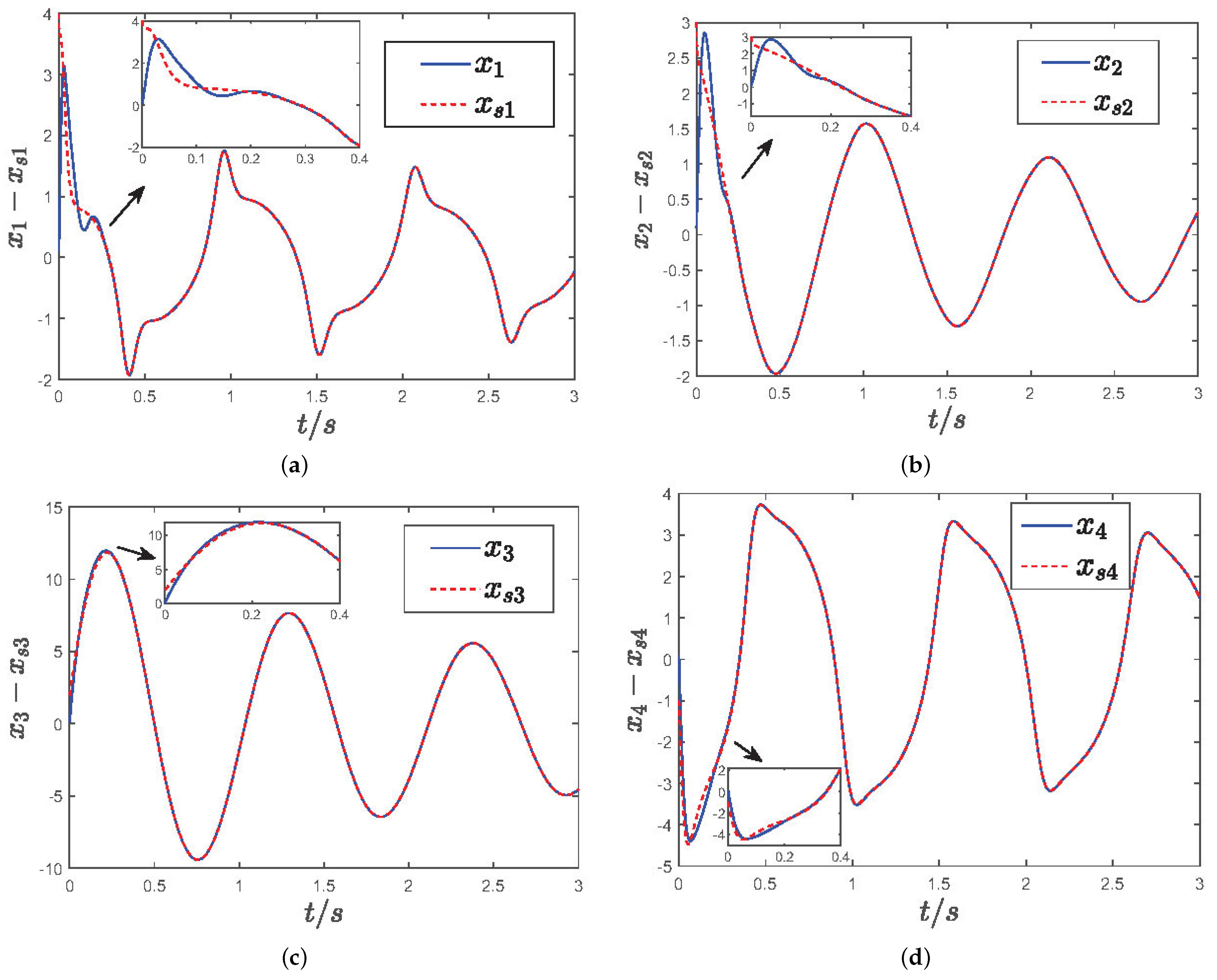
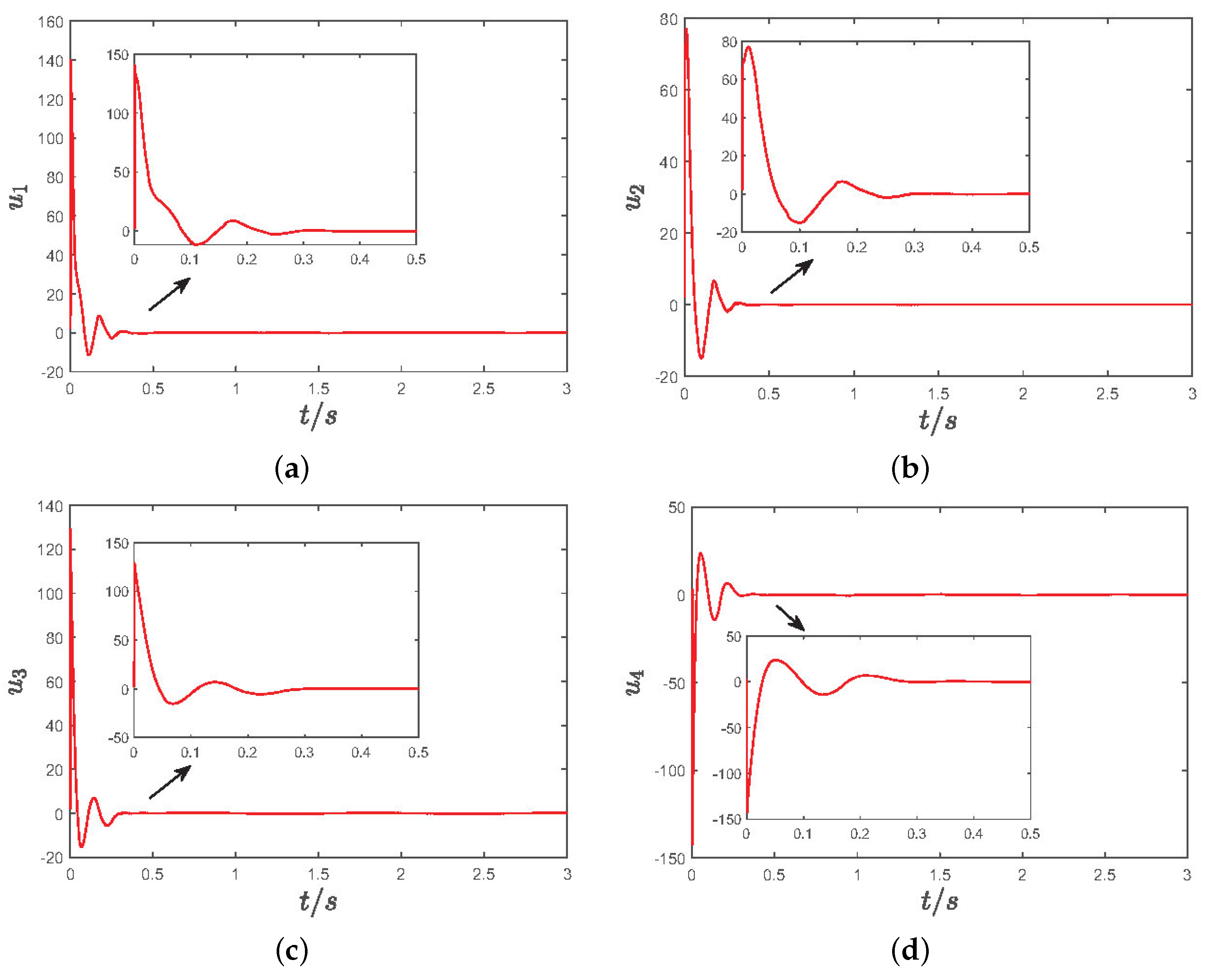
5.2. Simulation Results

In the numerical simulation of fixed-time synchronization control for incommensurate system, the system parameters are $a=3$, $b=12$, $c=2$, $d=32$, $e=-37$, $q_1=0.95$, $q_2=0.95$, $q_3=0.98$, and $q_4=0.98$. The initial value of the main system is $(0.1,0.1,0.1,0.1)$, the initial value of the follower system is $(4,3,2,-1)$. Furthermore, the uncertainties and disturbances contained in the leader system and follower system are as follows:

$$\left\{\begin{array}{c}\Delta f_1\left(x,t\right)=0.5cos\left(t\right)x_2,d_1^{f\left(t\right)}=sin\left(t\right)\hfill \\ \Delta f_2\left(x,t\right)=-0.5sin\left(t\right)x_3,d_2^{f\left(t\right)}=cos\left(5t\right)\hfill \\ \Delta f_3\left(x,t\right)=-0.3sin\left(t\right)x_2,d_3^{f\left(t\right)}=\mathrm{t}-\mathrm{round}\left(\mathrm{t}\right)\hfill \\ \Delta f_4\left(x,t\right)=0.1sin\left(t\right)x_4,d_4^{f\left(t\right)}=0.1sin\left(2t\right)\hfill \\ \Delta g_{s1}\left(x,t\right)=0.5cos\left(t\right)x_{s2},d_{s1}^{g\left(t\right)}=sign\left(cos\left(t\right)\right)\hfill \\ \Delta g_{s2}\left(x,t\right)=0.2sin\left(t\right)x_{s3},d_{s1}^{g\left(t\right)}=\mathrm{t}-\mathrm{round}\left(\mathrm{t}\right)\hfill \\ \Delta g_{s3}\left(x,t\right)=0.2cos\left(2t\right)x_{s2},d_{s3}^{g\left(t\right)}=0.2sin\left(2t\right)\hfill \\ \Delta g_{s4}\left(x,t\right)=0.1sin\left(t\right)x_{s4},d_{s4}^{g\left(t\right)}=\mathrm{t}-\mathrm{round}\left(3\mathrm{t}\right)\hfill \end{array}\right.$$

(61)

We select the control parameters of the incommensurate system as ${\sigma }_1={\sigma }_2=10$, ${\eta }_1={\eta }_2=10$, ${\upsilon }_1={\upsilon }_2=9$, ${\vartheta }_1={\vartheta }_2=5$, ${\varsigma }_1={\varsigma }_2=5$, and ${\zeta }_1={\zeta }_2=9$. In the numerical simulation results, the behavior of the incommensurate system is illustrated in Figure 15, Figure 16 and Figure 17.

As shown in Figure 15, the incommensurate follower system progressively follows the motion trajectory of the leader system within 0.3 s. This observation demonstrates that the proposed fixed-time synchronization control scheme possesses excellent synchronization performance. According to Equation (60), the upper bound of the convergence time for the fixed-time synchronization control scheme is calculated to be $T=0.78\mathrm{s}$. This theoretical value aligns well with the synchronization time observed in the simulations, further validating the feasibility and effectiveness of the proposed control scheme. Figure 16 presents the control input curve. It is evident that the curve is smooth, with no noticeable chattering phenomenon. The smoothness of the control input curve indicates that the proposed control scheme effectively mitigates non-singular issues, significantly reducing or eliminating chattering. This enhancement leads to improved system stability and higher control precision. Figure 17 displays the sliding surface motion curve, which reflects the convergence speed of the fixed-time synchronization control scheme. From the sliding surface motion curve, it is clear that the system state rapidly approaches the sliding surface and achieves a stable state within a fixed time. In summary, these numerical simulation results comprehensively validate the effectiveness and practicality of the fixed-time synchronization control scheme, providing strong theoretical and empirical support for its application in real-world scenarios.

6. Conclusions

In this paper, the detailed description and calculation process of Adomian decomposition algorithm for incommensurate fractional-order chaotic system is given by using fractional calculus theory. On this basis, the phase diagrams, Poincaré section, coexistence bifurcation diagrams, and coexistence Lyapunov exponent spectrum are studied. Firstly, it is found that different fractional orders change lead to richer dynamic phenomena in the incommensurate system. Secondly, according to the coexistence bifurcation diagrams and the coexistence Lyapunov exponent spectrum, it is found that there are many types of coexistence attractors in the incommensurate system. Furthermore, it is found that it has a special chaotic degenerate dynamic behavior. At the same time, in order to illustrate the feasibility of the practical application of the incommensurate fractional-order system, the equivalent analog circuit of the incommensurate fractional-order chaotic system is designed. By capturing the chaotic attractors in the analog oscilloscope, it is found that its numerical simulation results are consistent. Finally, a fixed-time synchronization control scheme is designed, which can not only realize the synchronization control of incommensurate fractional-order chaotic systems, but also know that the upper limit of the synchronization control convergence time is independent of the initial conditions and the convergence time is fixed. Therefore, the research results in this paper will provide a new way for the practical application of incommensurate fractional-order chaotic systems.

References

1. Lin, H.; Wang, C.; Cui, L.; Sun, Y.; Zhang, X.; Yao, W. Hyperchaotic memristive ring neural network and application in medical image encryption. Nonlinear Dyn. 2022, 110, 841–855. [Google Scholar] [CrossRef]
2. Yang, J.; Xiong, J.; Cen, J.; He, W. Finite-time generalized synchronization of non-identical fractional order chaotic systems and its application in speech secure communication. PLoS ONE 2022, 17, e0263007. [Google Scholar] [CrossRef]
3. Wang, Z.; Hu, W. Chaos of a single-walled carbon nanotube resulting from periodic parameter perturbation. Int. J. Bifurc. Chaos 2021, 31, 2150130. [Google Scholar] [CrossRef]
4. Wang, Z.; Hu, W. Resonance analysis of a single-walled carbon nanotube. Chaos Solitons Fractals 2021, 142, 110498. [Google Scholar] [CrossRef]
5. Wang, Z.; Yang, Y.; Parastesh, F.; Cao, S.; Wang, J. Chaotic dynamics of a carbon nanotube oscillator with symmetry-breaking. Phys. Scr. 2025, 100, 015225. [Google Scholar] [CrossRef]
6. Tian, H.; Wang, Z.; Zhang, H.; Cao, Z.; Zhang, P. Dynamical analysis and fixed-time synchronization of a chaotic system with hidden attractor and a line equilibrium. Eur. Phys. J. Spec. Top. 2022, 231, 2455–2466. [Google Scholar] [CrossRef]
7. Tian, H.; Zhao, M.; Liu, J.; Wang, Q.; Yu, X.; Wang, Z. Dynamic Analysis and Sliding Mode Synchronization Control of Chaotic Systems with Conditional Symmetric Fractional-Order Memristors. Fractal Fract. 2024, 8, 307. [Google Scholar] [CrossRef]
8. Li, G.; Xu, X.; Zhong, H. A image encryption algorithm based on coexisting multi-attractors in a spherical chaotic system. Multimed. Tools Appl. 2022, 81, 32005–32031. [Google Scholar] [CrossRef]
9. Yang, N.; Xu, C.; Wu, C.; Jia, R.; Liu, C. Modeling and analysis of a fractional-order generalized memristor-based chaotic system and circuit implementation. Int. J. Bifurc. Chaos 2017, 27, 1750199. [Google Scholar] [CrossRef]
10. Said, L.A.; Radwan, A.G.; Madian, A.H.; Soliman, A.M. Three fractional-order-capacitors-based oscillators with controllable phase and frequency. J. Circuits Syst. Comput. 2017, 26, 1750160. [Google Scholar] [CrossRef]
11. Ghanbari, B.; Atangana, A. A new application of fractional Atangana–Baleanu derivatives: Designing ABC-fractional masks in image processing. Phys. A Stat. Mech. Its Appl. 2020, 542, 123516. [Google Scholar] [CrossRef]
12. Jahanshahi, H.; Yousefpour, A.; Munoz-Pacheco, J.M.; Kacar, S.; Pham, V.T.; Alsaadi, F.E. A new fractional-order hyperchaotic memristor oscillator: Dynamic analysis, robust adaptive synchronization, and its application to voice encryption. Appl. Math. Comput. 2020, 383, 125310. [Google Scholar] [CrossRef]
13. Qureshi, S.; Yusuf, A.; Shaikh, A.A.; Inc, M.; Baleanu, D. Fractional modeling of blood ethanol concentration system with real data application. Chaos Interdiscip. J. Nonlinear Sci. 2019, 29, 013143. [Google Scholar] [CrossRef] [PubMed]
14. Yusuf, A.; Qureshi, S.; Inc, M.; Aliyu, A.I.; Baleanu, D.; Shaikh, A.A. Two-strain epidemic model involving fractional derivative with Mittag-Leffler kernel. Chaos Interdiscip. J. Nonlinear Sci. 2018, 28, 123121. [Google Scholar] [CrossRef] [PubMed]
15. Xu, Y.; Sun, K.; He, S.; Zhang, L. Dynamics of a fractional-order simplified unified system based on the Adomian decomposition method. Eur. Phys. J. Plus 2016, 131, 186. [Google Scholar] [CrossRef]
16. Gul, T.; Alghamdi, W.; Khan, I.; Ali, I. New similarity variable to transform the fluid flow from PDEs into fractional-order ODEs: Numerical study. Phys. Scr. 2021, 96, 084009. [Google Scholar] [CrossRef]
17. Danca, M.F. Hopfield neuronal network of fractional order: A note on its numerical integration. Chaos Solitons Fractals 2021, 151, 111219. [Google Scholar] [CrossRef]
18. Ramani, P.; Khan, A.M.; Suthar, D.L.; Kumar, D. Approximate analytical solution for non-linear Fitzhugh–Nagumo equation of time fractional order through fractional reduced differential transform method. Int. J. Appl. Comput. Math. 2022, 8, 61. [Google Scholar] [CrossRef]
19. Atangana, A.; Araz, S. New numerical approximation for Chua attractor with fractional and fractal-fractional operators. Alex. Eng. J. 2020, 59, 3275–3296. [Google Scholar] [CrossRef]
20. Atangana, A.; Araz, S.İ. Fractional stochastic modelling illustration with modified Chua attractor. Eur. Phys. J. Plus 2019, 134, 160. [Google Scholar] [CrossRef]
21. Wang, Z.; Sun, W.; Wei, Z.; Zhang, S. Dynamics and delayed feedback control for a 3D jerk system with hidden attractor. Nonlinear Dyn. 2015, 82, 577–588. [Google Scholar] [CrossRef]
22. Wang, Z.; Wei, Z.; Xi, X.; Li, Y. Dynamics of a 3D autonomous quadratic system with an invariant algebraic surface. Nonlinear Dyn. 2014, 77, 1503–1518. [Google Scholar] [CrossRef]
23. Chen, C.; Min, F. ReLU-type memristor-based Hopfield neural network. Eur. Phys. J. Spec. Top. 2022, 231, 2979–2992. [Google Scholar] [CrossRef]
24. Chang, H.; Li, Y.; Chen, G.; Yuan, F. Extreme multistability and complex dynamics of a memristor-based chaotic system. Int. J. Bifurc. Chaos 2020, 30, 2030019. [Google Scholar] [CrossRef]
25. Al-Nassir, S. Dynamic analysis of a harvested fractional-order biological system with its discretization. Chaos Solitons Fractals 2021, 152, 111308. [Google Scholar] [CrossRef]
26. Ma, C.; Mou, J.; Yang, F.; Yan, H. A fractional-order hopfield neural network chaotic system and its circuit realization. Eur. Phys. J. Plus 2020, 135, 100. [Google Scholar] [CrossRef]
27. Tavazoei, M.S.; Haeri, M. Synchronization of chaotic fractional-order systems via active sliding mode controller. Phys. A Stat. Mech. Its Appl. 2008, 387, 57–70. [Google Scholar] [CrossRef]
28. Almatroud, A.O. On the anti-synchronization of fractional-order chaotic and hyperchaotic systems via modified adaptive sliding-mode control. Turk. J. Comput. Math. Educ. (TURCOMAT) 2021, 12, 1112–1123. [Google Scholar]
29. Chen, L.; Fang, J.A. Adaptive continuous sliding mode control for fractional-order systems with uncertainties and unknown control gains. Int. J. Control Autom. Syst. 2022, 20, 1509–1520. [Google Scholar] [CrossRef]
30. Zambrano-Serrano, E.; Bekiros, S.; Platas-Garza, M.A.; Posadas-Castillo, C.; Agarwal, P.; Jahanshahi, H.; Aly, A.A. On chaos and projective synchronization of a fractional difference map with no equilibria using a fuzzy-based state feedback control. Phys. A Stat. Mech. Its Appl. 2021, 578, 126100. [Google Scholar] [CrossRef]
31. Wang, L.; Dong, J. Reset event-triggered adaptive fuzzy consensus for nonlinear fractional-order multiagent systems with actuator faults. IEEE Trans. Cybern. 2022, 53, 1868–1879. [Google Scholar] [CrossRef] [PubMed]
32. Alattas, K.A.; Mostafaee, J.; Sambas, A.; Alanazi, A.K.; Mobayen, S.; Vu, M.T.; Zhilenkov, A. Nonsingular integral-type dynamic finite-time synchronization for hyper-chaotic systems. Mathematics 2021, 10, 115. [Google Scholar] [CrossRef]
33. Aghababa, M.P. Design of a chatter-free terminal sliding mode controller for nonlinear fractional-order dynamical systems. Int. J. Control 2013, 86, 1744–1756. [Google Scholar] [CrossRef]
34. Wang, Y.L.; Jahanshahi, H.; Bekiros, S.; Bezzina, F.; Chu, Y.M.; Aly, A.A. Deep recurrent neural networks with finite-time terminal sliding mode control for a chaotic fractional-order financial system with market confidence. Chaos Solitons Fractals 2021, 146, 110881. [Google Scholar] [CrossRef]
35. Ni, J.; Liu, L.; Liu, C.; Hu, X. Fractional order fixed-time nonsingular terminal sliding mode synchronization and control of fractional order chaotic systems. Nonlinear Dyn. 2017, 89, 2065–2083. [Google Scholar] [CrossRef]
36. Wang, C.; Liu, C.L.; Chen, Y.Y.; Zhang, Y. Fixed-time consensus tracking for second-order leader-follower multi-agent systems with nonlinear dynamics under directed topology. Int. J. Control Autom. Syst. 2021, 19, 2697–2705. [Google Scholar] [CrossRef]
37. Wang, Z.; Parastesh, F.; Natiq, H.; Li, J.; Xi, X.; Mehrabbeik, M. Synchronization patterns in a network of diffusively delay-coupled memristive Chialvo neuron map. Phys. Lett. A 2024, 514, 129607. [Google Scholar] [CrossRef]
38. Wang, Z.; Chen, M.; Xi, X.; Tian, H.; Yang, R. Multi-chimera states in a higher order network of FitzHugh–Nagumo oscillators. Eur. Phys. J. Spec. Top. 2024, 233, 779–786. [Google Scholar] [CrossRef]
39. Delgado, B.B.; Macías-Díaz, J.E. On the general solutions of some non-homogeneous Div-Curl systems with Riemann–Liouville and Caputo fractional derivatives. Fractal Fract. 2021, 5, 117. [Google Scholar] [CrossRef]
40. Yusuf, A.; Acay, B.; Inc, M. Analysis of fractional-order nonlinear dynamic systems under Caputo differential operator. Math. Methods Appl. Sci. 2021, 44, 10861–10880. [Google Scholar] [CrossRef]
41. Liu, J.; Wang, Z.; Chen, M.; Zhang, P.; Yang, R.; Yang, B. Chaotic system dynamics analysis and synchronization circuit realization of fractional-order memristor. Eur. Phys. J. Spec. Top. 2022, 231, 3095–3107. [Google Scholar] [CrossRef]
42. Cafagna, D.; Grassi, G. Hyperchaos in the fractional-order Rössler system with lowest-order. Int. J. Bifurc. Chaos 2009, 19, 339–347. [Google Scholar] [CrossRef]
43. Dutta, M.; Roy, B.K. A new memductance-based fractional-order chaotic system and its fixed-time synchronisation. Chaos Solitons Fractals 2021, 145, 110782. [Google Scholar] [CrossRef]
44. Hardy, G.H.; Littlewood, J.E.; Pólya, G. Inequalities; Cambridge University Press: Cambridge, UK, 1952. [Google Scholar]
45. He, X.; Li, X.; Song, S. Prescribed-time stabilization of nonlinear systems via impulsive regulation. IEEE Trans. Syst. Man, Cybern. Syst. 2022, 53, 981–985. [Google Scholar] [CrossRef]
Figure 1. (a) x 1 x 2 phase plane. (b) x 1 x 3 phase plane. (c) x 3 x 4 phase plane. (d) x 1 x 2 phase plane. (e) x 1 x 3 phase plane. (f) x 3 x 4 phase plane. Phase diagrams: (ac) q 1 = q 2 = q 3 = q 4 = 0.85 ; (df) q 1 = q 2 = q 3 = 0.70 , q 4 = 0.90 .
Fractalfract 09 00018 g001
Figure 2. Poincaré section of incommensurate system at x 2 = 0 . (a) Double-scroll Poincaré section. (b) Single-scroll Poincaré section.
Fractalfract 09 00018 g002
Figure 3. Bifurcation diagram and LEs of incommensurate system when q i ( 0.8 , 1 ) , i = 1 , 2 , 3 , 4 . (a) q 1 0.8 , 1 . (b) q 2 0.8 , 1 . (c) q 3 0.8 , 1 . (d) q 4 0.8 , 1 .
Fractalfract 09 00018 g003
Figure 4. Coexistence dynamics phenomenon of parameter a change. (a) Bifurcation of coexistence of initial values. (b) LEs of coexistence of initial values.
Fractalfract 09 00018 g004
Figure 5. Coexistence attractor types of incommensurate system with different parameter a in x 1 x 2 plane. (a) Symmetric periodic-1 coexistence attractors. (b) Symmetric periodic-2 coexistence attractors. (c) Symmetric periodic-4 coexistence attractor. (d) Symmetric single-scroll coexistence attractor. (e) Symmetric single-helix coexistence attractor. (f) Symmetric double-scroll coexistence attractor.
Fractalfract 09 00018 g005
Figure 6. Coexistence dynamics phenomenon of parameter b change. (a) Bifurcation of coexistence of initial values. (b) LEs of coexistence of initial values.
Fractalfract 09 00018 g006
Figure 7. Coexistence attractor types of incommensurate system with different parameter b in x 1 x 2 plane. (a) Symmetric periodic-1 coexistence attractors. (b) Symmetric periodic-2 coexistence attractors. (c) Symmetric periodic-4 coexistence attractors. (d) Symmetric single-scroll coexistence attractors. (e) Symmetric double-vortex period-1 attractors. (f) Symmetric double-vortex period-2 attractors.
Fractalfract 09 00018 g007
Figure 8. Coexistence dynamics phenomenon of parameter d change. (a) Bifurcation of coexistence of initial values. (b) LEs of coexistence of initial values.
Fractalfract 09 00018 g008
Figure 9. Coexistence attractor types of incommensurate system with different parameter d in x 1 x 2 plane. (a) Single-scroll coexistence attractors. (b) Periodic- and single-scroll coexisting attractors. (c) Single-vortex and periodic coexistence attractors. (d) Coexistence attractors of period-2 and period-4. (e) Symmetric period-2 attractors. (f) Symmetric period-1 attractors.
Fractalfract 09 00018 g009
Figure 10. Coexistence dynamics phenomenon of parameter f change. (a) Bifurcation of coexistence of initial values. (b) LEs of coexistence of initial values.
Fractalfract 09 00018 g010
Figure 11. Coexistence attractor types of incommensurate system with different parameter f in x 1 x 2 plane. (a) Symmetric periodic-1 coexistence attractors. (b) Symmetric periodic-2 coexistence attractors. (c) Symmetric periodic-4 coexistence attractors. (d) Coexistence attractors of single-scroll and limited cycles. (e) Single-scroll coexistence attractors. (f) Double-vortex period-1 coexistence attractors.
Fractalfract 09 00018 g011
Figure 12. Chaotic degeneration behavior of incommensurate system. (a) Time–domain waveform of state variable x 4 in time t (0–40 s). (b) Time–domain waveform of state variable x 4 in time t (30–40 s). (c) The phase diagram of transient double-scroll chaotic attractor in time t (0–20 s). (d) Phase diagram of stable periodic limit cycles in time t (20–40 s).
Fractalfract 09 00018 g012
Figure 13. Circuit schematic diagram of incommensurate system (13).
Fractalfract 09 00018 g013
Figure 14. Coexistence attractor types of incommensurate system with different parameter f in x 1 x 2 plane. (a) x 1 x 2 plane phase diagram. (b) x 1 x 3 plane phase diagram. (c) x 3 x 4 plane phase diagram.
Fractalfract 09 00018 g014
Figure 15. Synchronization curve of state variables for incommensurate system. (a) Synchronization curve of state variables x 1 and x s 1 . (b) Synchronization curve of state variables x 2 and x s 2 . (c) Synchronization curve of state variables x 3 and x s 3 . (d) Synchronization curve of state variables x 4 and x s 4 .
Fractalfract 09 00018 g015
Figure 16. Control input curve of incommensurate system. (a) Control input u 1 curve. (b) Control input u 2 curve. (c) Control input u 3 curve. (d) Control input u 4 curve.
Fractalfract 09 00018 g016
Figure 17. Incommensurate system sliding surface motion curve. (a) s 1 sliding surface curve. (b) s 2 sliding surface curve. (c) s 3 sliding surface curve. (d) s 4 sliding surface curve.
Fractalfract 09 00018 g017
Disclaimer/Publisher’s Note: The statements, opinions and data contained in all publications are solely those of the individual author(s) and contributor(s) and not of MDPI and/or the editor(s). MDPI and/or the editor(s) disclaim responsibility for any injury to people or property resulting from any ideas, methods, instructions or products referred to in the content.