Article

A High-Order Numerical Method Based on a Spatial Compact Exponential Scheme for Solving the Time-Fractional Black–Scholes Model

School of Mathematics and Statistics, Shandong University, Weihai 264209, China
*
Author to whom correspondence should be addressed.
Fractal Fract. 2024, 8(8), 465; https://doi.org/10.3390/fractalfract8080465
Submission received: 10 July 2024 / Revised: 1 August 2024 / Accepted: 5 August 2024 / Published: 7 August 2024

Abstract

This paper investigates a high-order numerical method based on a spatial compact exponential scheme for solving the time-fractional Black–Scholes model. Firstly, the original time-fractional Black–Scholes model is converted into an equivalent time-fractional advection–diffusion reaction model by means of a variable transformation technique. Secondly, a novel high-order numerical method is constructed with ( 2 α ) accuracy in time and fourth-order accuracy in space based on a spatial compact exponential scheme, where α is the fractional derivative. The uniqueness of solvability of the derived numerical method is rigorously discussed. Thirdly, the unconditional stability and convergence of the derived numerical method are rigorously analyzed using the Fourier analysis technique. Finally, numerical examples are presented to test the effectiveness of the derived numerical method. The proposed numerical method is also applied to solve the time-fractional Black–Scholes model, whose exact analytical solution is unknown; numerical results are illustrated graphically.

1. Introduction

Due to the nonlocal nature of the fractional differential and integral operators, fractional calculus has gained more and more attention from researchers. Fractional calculus has provided a powerful tool for modeling anomalous behaviours from various fields of science and engineering, such as material science, biology, physics, control science, fluid mechanics and finance [1,2,3].
In the financial market, the famous Black–Scholes model [4,5] was derived to determine the option price under some strict assumptions. However, the model still has some drawbacks; for example, it cannot capture some significant movements or jumps within a small time step [6]. Hence, the Black–Scholes model does not often show the actual performance of stock prices in a realistic financial market. Since the fractional differential and integral operators make it easy to characterize the behaviors with memory and hereditary properties, the fractional Black–Scholes model was generalized [7,8]. Liang et al. [9] established a novel two-parameter time-fractional Black–Scholes-Merton model for option pricing. Chen et al. [10] considered the variation in the option price as a fractal transmission system and derived a time-fractional Black–Scholes model. Zhang et al. [11] gave a comprehensive review for various fractional Black–Scholes equations.
Since the exact solutions for various kinds of fractional partial differential equations are not often available, numerical methods for solving these equations must be considered. Various efficient numerical methods have already been investigated [12,13,14,15,16,17], such as finite difference methods, finite volume methods, finite element methods and spectral methods. For the time-fractional Black–Scholes model, Zhang et al. [6] constructed a numerical scheme with ( 2 α ) accuracy in time and second-order spatial accuracy, and analyzed the stability and convergence. Soon, De Staelen and Hendy [18] constructed a high-order difference method with fourth-order spatial accuracy, and analyzed the stability and convergence. Similar results can be found in [19]. Roul [20] constructed a numerical method based on a B-spline collocation technique. An et al. [21] presented a space–time spectral method and analyzed the stability and convergence of the numerical method. Song and Lyu [22] investigated a high-order and fast numerical method for the time-fractional Black–Scholes equation, with a weak initial singularity of the solution. Abdi et al. [23] introduced two compact finite difference methods. Taghipour and Aminikhah [24] proposed an efficient spectral collocation method. Kaur and Natesan [25] proposed a numerical method based on the cubic spline method. Zhang and Zheng [26] proposed the finite element method for solving the variable-order time-fractional Black–Scholes model. Kazmi [27] developed an efficient numerical method with second-order temporal and spatial accuracy.
In this paper, we investigate the following time-fractional Black–Scholes model [10]:
α V ( S , τ ) τ α + 1 2 σ 2 S 2 2 V ( S , τ ) S 2 + r S V ( S , τ ) S r V ( S , τ ) = 0 , ( S , τ ) ( 0 , ) × ( 0 , T ) , V ( 0 , τ ) = p ˜ ( τ ) , V ( , τ ) = q ˜ ( τ ) , V ( S , T ) = ψ ˜ ( S ) ,
where V ( S , τ ) represents the price of an option, S is the asset price, τ is the current time, σ is the volatility of the underlying asset, r is the risk-free interest rate, T is the expiry time, the function ψ ˜ ( S ) is the terminal condition which denotes the terminal payoff function of the option, and the functions p ˜ ( τ ) and q ˜ ( τ ) are boundary conditions which denote the rebates paid when the corresponding barrier is hit [10]; more details can be found in [10]. The time-fractional derivative α V ( S , τ ) τ α in model (1) is the modified right Riemann–Liouville time-fractional derivative
α V ( S , τ ) τ α = 1 Γ ( 1 α ) d d τ τ T V ( S , ξ ) V ( S , T ) ( ξ τ ) α d ξ , 0 < α < 1 , V ( S , τ ) τ , α = 1 .
When the fractional derivative α = 1 , the above mentioned model (1) becomes the classical Black–Scholes model. While 0 < α < 1 , the above mentioned model (1) represents a time-fractional Black–Scholes model [10]. An example describing the European double barrier knock-out call option can be found in Section 4.
Letting S = e x and τ = T t , and denoting u ( x , t ) = V e x , T t , the above mentioned time-fractional Black–Scholes model (1) can be rewritten as
  0 D t α u ( x , t ) = 1 2 σ 2 2 u ( x , t ) x 2 + r 1 2 σ 2 u ( x , t ) x r u ( x , t ) , u ( , t ) = p ( t ) , u ( , t ) = q ( t ) , 0 t T , u ( x , 0 ) = ψ ( x ) ,
and the time-fractional derivative α V ( S , τ ) τ α is transformed into the following form:
  0 D t α u ( x , t ) = 1 Γ ( 1 α ) d d t 0 t u ( x , η ) u ( x , 0 ) ( t η ) α d η , 0 < α < 1 .
Actually, the fractional derivative   0 D t α u ( x , t ) in model (3) represents the Caputo time-fractional derivative   0 C D t α u ( x , t ) which is already derived in reference [6,10]
  0 D t α u ( x , t ) = 1 Γ ( 1 α ) d d t 0 t u ( x , η ) ( t η ) α d η 1 Γ ( 1 α ) d d t 0 t u ( x , 0 ) ( t η ) α d η = 1 Γ ( 1 α ) 0 t ( t η ) α u ( x , η ) η d η + u ( x , 0 ) t α Γ ( 1 α ) u ( x , 0 ) t α Γ ( 1 α ) = 1 Γ ( 1 α ) 0 t ( t η ) α u ( x , η ) η d η =   0 C D t α u ( x , t ) .
In order to obtain the numerical solution of the above time-fractional Black–Scholes model (3), it is necessary to truncate the original unbounded domain ( 0 , ) × ( 0 , T ) into a finite domain ( x L , x R ) × ( 0 , T ) . Hence, the aim of this paper is to investigate the following time-fractional advection–diffusion reaction model:
  0 C D t α u ( x , t ) = a 2 u ( x , t ) x 2 + b u ( x , t ) x c u ( x , t ) + f ( x , t ) , ( x , t ) ( x L , x R ) × ( 0 , T ) , u x L , t = p ( t ) , u x R , t = q ( t ) , 0 t T , u ( x , 0 ) = ψ ( x ) , x L x x R ,
where a = 1 2 σ 2 > 0 , b = r 1 2 σ 2 = r a , c = r > 0 , the function f ( x , t ) as a source term is added for numerical experimental validation.
The outline of the paper is arranged as follows. In Section 2, a high-order numerical method is derived with ( 2 α ) temporal accuracy and fourth-order spatial accuracy, and the uniqueness of solvability is rigorously discussed. In Section 3, the stability and the convergence of the derived high-order numerical method is strictly analyzed using the Fourier analysis technique. In Section 4, numerical examples are given to test the effectiveness of the proposed numerical method. The proposed numerical method is also applied to solve the time-fractional Black–Scholes model, whose exact analytical solution is unknown; the call option prices for different fractional derivative α are illustrated graphically. Finally, some conclusions are summarized.

2. Construction of the High-Order Numerical Method

In this section, we will derive a high-order numerical method based on a spatial compact exponential scheme for the derived fractional advection–diffusion reaction model (6).
Firstly, let M and N be two positive integers, h = x R x L M the space step, and Δ t = T N the time step. Denote Ω h = { x j | x j = x L + j h , j = 0 , 1 , 2 , , M } and Ω τ = { t n | t n = n Δ t , n = 0 , 1 , 2 , , N } . Denote the grid function u j n = u ( x j , t n ) and f j n = f ( x j , t n ) .
Introduce the following notations:
δ x 2 u j n = u j 1 n 2 u j n + u j + 1 n h 2 , δ x u j n = u j + 1 n u j 1 n 2 h .
In order to derive a high-order numerical discrete scheme in space, we first investigate the corresponding convection–diffusion equation
a 2 u ( x , t ) x 2 + b u ( x , t ) x = g ( x , t ) ,
where g ( x , t ) is a suitable smooth function. A fourth-order compact exponential scheme has already been derived [28,29]
B u j = A g j + O ( h 4 ) ,
where
A = 1 + α 1 δ x + α 2 δ x 2 , B = β δ x 2 + b δ x ,
with
β = b h 2 coth b h 2 a , α 1 = a β b , α 2 = a ( a + β ) b 2 + h 2 6 .
Substituting g ( x , t ) =   0 C D t α u ( x , t ) + c u ( x , t ) f ( x , t ) in the Equation (9) at the mesh point ( x j , t n ) , we can obtain the following semi-discrete high-order compact exponential approximation scheme:
β h 2 b 2 h u j 1 n + 2 β h 2 u j n + β h 2 + b 2 h u j + 1 n = α 1 2 h + α 2 h 2   0 C D t α u + c u f j 1 n + 1 2 α 2 h 2   0 C D t α u + c u f j n + α 1 2 h + α 2 h 2   0 C D t α u + c u f j + 1 n + O ( h 4 ) .
Next, in order to construct a fully-discrete numerical approximation method, we introduce the following two lemmas:
Lemma 1 
([30]). Assuming that f ( t ) C 2 0 , t n , let
R ¯ f t n = 1 Γ ( 1 α ) 0 t n f ( s ) t n s α d s Δ t α Γ ( 2 α ) a 0 f t n k = 1 n 1 a n k 1 a n k f t k a n 1 f t 0 ,
then
R ¯ f t n 1 Γ ( 2 α ) 1 α 12 + 2 2 α 2 α 1 + 2 α max 0 t t n f ( t ) Δ t 2 α ,
where α ( 0 , 1 ) and a n = ( n + 1 ) 1 α n 1 α ( n = 0 , 1 , 2 , 3 , ) .
Lemma 2. 
The coefficients a n ( n = 0 , 1 , 2 , 3 , ) in (13) satisfy
( 1 ) 1 = a 0 > a 1 > a 2 > > a n > , ( 2 ) a n 0 ( n ) .
From Lemma 1, it is known that the Caputo time-fractional derivative   0 C D t α u ( x , t ) ( 0 < α < 1 ) can be discretized at the point ( x j , t n ) by
  0 C D t α u ( x j , t n ) = Δ t α Γ ( 2 α ) a 0 u j n k = 1 n 1 a n k 1 a n k u j k a n 1 u j 0 + O ( Δ t 2 α ) .
Substituting (15) into (12) and denoting μ = Δ t α Γ ( 2 α ) , we can obtain that, for n = 1 ,
( c + μ ) α 1 2 h + α 2 h 2 + β h 2 + b 2 h u j 1 1 + ( c + μ ) 1 2 α 2 h 2 2 β h 2 u j 1 + ( c + μ ) α 1 2 h + α 2 h 2 + β h 2 b 2 h u j + 1 1 = μ α 1 2 h + α 2 h 2 u j 1 0 + 1 2 α 2 h 2 u j 0 + α 1 2 h + α 2 h 2 u j + 1 0 + α 1 2 h + α 2 h 2 f j 1 1 + 1 2 α 2 h 2 f j 1 + α 1 2 h + α 2 h 2 f j + 1 1 + R j 1 , 1 j M 1 ,
and, for n 2 ,
( c + μ ) α 1 2 h + α 2 h 2 + β h 2 + b 2 h u j 1 n + ( c + μ ) 1 2 α 2 h 2 2 β h 2 u j n + ( c + μ ) α 1 2 h + α 2 h 2 + β h 2 b 2 h u j + 1 n = μ k = 1 n 1 a n k 1 a n k α 1 2 h + α 2 h 2 u j 1 k + 1 2 α 2 h 2 u j k + α 1 2 h + α 2 h 2 u j + 1 k + μ a n 1 α 1 2 h + α 2 h 2 u j 1 0 + 1 2 α 2 h 2 u j 0 + α 1 2 h + α 2 h 2 u j + 1 0 + α 1 2 h + α 2 h 2 f j 1 n + 1 2 α 2 h 2 f j n + α 1 2 h + α 2 h 2 f j + 1 n + R j n , 1 j M 1 ,
where R j n = O ( Δ t 2 α + h 4 ) , that is, there exists a constant C 1 > 0 , such that
R j n C 1 Δ t 2 α + h 4 .
Substituting u j n with its numerical approximations U j n and omitting R j n , we have derived a high-order numerical scheme as follows:
( c + μ ) α 1 2 h + α 2 h 2 + β h 2 + b 2 h U j 1 1 + ( c + μ ) 1 2 α 2 h 2 2 β h 2 U j 1 + ( c + μ ) α 1 2 h + α 2 h 2 + β h 2 b 2 h U j + 1 1 = μ α 1 2 h + α 2 h 2 U j 1 0 + 1 2 α 2 h 2 U j 0 + α 1 2 h + α 2 h 2 U j + 1 0 + α 1 2 h + α 2 h 2 f j 1 1 + 1 2 α 2 h 2 f j 1 + α 1 2 h + α 2 h 2 f j + 1 1 , 1 j M 1 , n = 1 ,
and, for n 2 ,
( c + μ ) α 1 2 h + α 2 h 2 + β h 2 + b 2 h U j 1 n + ( c + μ ) 1 2 α 2 h 2 2 β h 2 U j n + ( c + μ ) α 1 2 h + α 2 h 2 + β h 2 b 2 h U j + 1 n = μ k = 1 n 1 a n k 1 a n k α 1 2 h + α 2 h 2 U j 1 k + 1 2 α 2 h 2 U j k + α 1 2 h + α 2 h 2 U j + 1 k + μ a n 1 α 1 2 h + α 2 h 2 U j 1 0 + 1 2 α 2 h 2 U j 0 + α 1 2 h + α 2 h 2 U j + 1 0 + α 1 2 h + α 2 h 2 f j 1 n + 1 2 α 2 h 2 f j n + α 1 2 h + α 2 h 2 f j + 1 n , 1 j M 1 .
Finally, we discretize the initial condition and the boundary conditions by
U 0 n = p ( t n ) , U M n = q ( t n ) , 1 n N ,
U j 0 = ψ ( x j ) , 0 j M .
Next, we will discuss the unique solvability of the derived numerical method (19)–(22).
Theorem 1. 
The derived numerical method (19)–(22) has a unique solution.
Proof. 
The matrix form of the derived numerical method (19)–(22) can be written as
P U n = l = 0 n 1 B l U l + F n ,
where
P = tridiag ( r 1 , r 2 , r 3 )
with
r 1 = ( c + μ ) α 1 2 h + α 2 h 2 + β h 2 + b 2 h ,
r 2 = ( c + μ ) 1 2 α 2 h 2 2 β h 2 ,
r 3 = ( c + μ ) α 1 2 h + α 2 h 2 + β h 2 b 2 h .
Noting that
β h 2 ± b 2 h = a h 2 b h 2 a coth b h 2 a ± b h 2 a = a h 2 b h 2 a coth b h 2 a ± 1 ,
and letting z = b h 2 a , we can obtain
b h 2 a coth b h 2 a ± 1 = 2 z e z e z e z = 2 e z z z 1 e 2 z 0 , z ( , + ) .
Therefore,
β h 2 + b 2 h + β h 2 b 2 h = 2 β h 2 .
Using Lemma 3 in [29], we can obtain
α 2 h 2 α 1 2 h + α 2 h 2 + α 1 2 h < 1 2 α 2 h 2 = 1 2 α 2 h 2 .
Therefore,
| r 1 | + | r 3 | = ( c + μ ) α 1 2 h + α 2 h 2 + β h 2 + b 2 h + ( c + μ ) α 1 2 h + α 2 h 2 + β h 2 b 2 h ( c + μ ) α 1 2 h + α 2 h 2 + α 1 2 h + α 2 h 2 + β h 2 + b 2 h + β h 2 b 2 h < ( c + μ ) 1 2 α 2 h 2 2 β h 2 = | r 2 | ,
which means the coefficient matrix P is a strictly diagonal dominant matrix, hence, matrix P is non-singular. Therefore, the solution is unique. □

3. Stability and Convergence Analysis

For the derived high-order numerical method (19)–(22), the stability and convergence analysis will be rigorously discussed by the Fourier analysis method.

3.1. Stability Analysis

For simplicity, we first denote
s 1 = α 1 2 h + α 2 h 2 , s 2 = 1 2 α 2 h 2 , s 3 = α 1 2 h + α 2 h 2 ,
and r 1 , r 2 , r 3 are already denoted in (25)–(27).
Suppose that U ˜ j n is the approximation solution of the above numerical scheme (19)–(22). Let
ρ j n = U j n U ˜ j n , 1 j M 1 , 0 n N ,
with ρ 0 n = ρ M n = 0 , and ρ n = ρ 1 n , ρ 2 n , , ρ M 1 n T . Therefore, we can obtain that, for n = 1 ,
r 1 ρ j 1 1 + r 2 ρ j 1 + r 3 ρ j + 1 1 = μ s 1 ρ j 1 0 + s 2 ρ j 0 + s 3 ρ j + 1 0 ,
and, for n 2 , we have
r 1 ρ j 1 n + r 2 ρ j n + r 3 ρ j + 1 n = μ k = 1 n 1 a n k 1 a n k s 1 ρ j 1 k + s 2 ρ j k + s 3 ρ j + 1 k + μ a n 1 s 1 ρ j 1 0 + s 2 ρ j 0 + s 3 ρ j + 1 0 .
Define the grid function
ρ n ( x ) = ρ j n , x j 1 2 < x x j + 1 2 , 1 j M 1 , 0 , x L x x L + h 2 or x R h 2 < x x R ,
and periodically expand ρ n ( x ) in the Fourier series [6] with the period L = x R x L
ρ n ( x ) = l = ξ n ( l ) e 2 π i l x / L ,
where
ξ n ( l ) = 1 L 0 L ρ n ( x ) e 2 π i l x / L d x .
Using the Parseval equality
0 L ρ n ( x ) 2 d x = l = ξ n ( l ) 2 ,
and the following discrete norm
ρ n 2 2 = j = 1 M 1 h ρ j n 2 ,
we have
ρ n 2 2 = j = 1 M 1 h ρ j n 2 = 0 L ρ n ( x ) 2 d x = l = ξ n ( l ) 2 .
Based on the above analysis, we assume that the solution of the above error Equations (31) and (32) has the expression
ρ j n = ξ n e i σ x L + j h
where σ = 2 π l / L .
Substituting the expression (35) into (31) and (32), we have
ξ 1 = μ s 1 + s 3 cos σ h + s 2 i s 1 s 3 sin σ h r 1 + r 3 cos σ h + r 2 i r 1 r 3 sin σ h ξ 0 , n = 1 ,
and, for n 2 ,
ξ n = 1 r 1 + r 3 cos σ h + r 2 i r 1 r 3 sin σ h × [ μ k = 1 n 1 a n k 1 a n k s 1 + s 3 cos σ h + s 2 i s 1 s 3 sin σ h ξ k + μ a n 1 s 1 + s 3 cos σ h + s 2 i s 1 s 3 sin σ h ξ 0 ] .
Lemma 3 
([29]). Assuming that z ( , ) , we have
z coth z 1 .
Lemma 4. 
The following inequality is established:
μ s 1 + s 3 cos σ h + s 2 i s 1 s 3 sin σ h r 1 + r 3 cos σ h + r 2 i r 1 r 3 sin σ h 1 .
Proof. 
Obviously, we have
μ s 1 + s 3 cos σ h + s 2 i s 1 s 3 sin σ h r 1 + r 3 cos σ h + r 2 i r 1 r 3 sin σ h 1 μ s 1 + s 3 cos σ h + s 2 i s 1 s 3 sin σ h r 1 + r 3 cos σ h + r 2 i r 1 r 3 sin σ h μ 2 α 2 h 2 cos σ h + 1 2 α 2 h 2 + i α 1 h sin σ h | ( c + μ ) 2 α 2 h 2 + 2 β h 2 cos σ h + ( c + μ ) 1 2 α 2 h 2 2 β h 2 + i ( c + μ ) α 1 h b h sin σ h | μ 2 1 2 α 2 h 2 ( 1 cos σ h ) 2 + α 1 2 h 2 sin 2 σ h ( c + μ ) 1 2 α 2 h 2 ( 1 cos σ h ) + 2 β h 2 ( cos σ h 1 ) 2 + ( c + μ ) α 1 h b h 2 sin 2 σ h ( c 2 + 2 c μ ) 1 2 α 2 h 2 ( 1 cos σ h ) 2 + 4 β 2 h 4 ( cos σ h 1 ) 2 + 2 ( c + μ ) 1 2 α 2 h 2 ( 1 cos σ h ) 2 β h 2 ( cos σ h 1 ) + ( c 2 + 2 c μ ) α 1 2 h 2 sin 2 σ h 2 ( c + μ ) α 1 h b h sin 2 σ h + b 2 h 2 sin 2 σ h 0 .
Since c > 0 , μ > 0 , then
( c 2 + 2 c μ ) 1 2 α 2 h 2 ( 1 cos σ h ) 2 0 , 4 β 2 h 4 ( cos σ h 1 ) 2 0 , ( c 2 + 2 c μ ) α 1 2 h 2 sin 2 σ h 0 , b 2 h 2 sin 2 σ h 0 .
Therefore, if we can prove
2 ( c + μ ) 1 2 α 2 h 2 ( 1 cos σ h ) 2 β h 2 ( cos σ h 1 ) 2 ( c + μ ) α 1 h b h sin 2 σ h 0 ,
that is
8 ( c + μ ) h 2 sin 2 σ h 2 β 1 4 α 2 h 2 sin 2 σ h 2 + b α 1 cos 2 σ h 2 0 ,
then (40) holds.
Next, if sin 2 σ h 2 = 0 , then (42) holds. While sin 2 σ h 2 0 , noticing that
β 1 4 α 2 h 2 sin 2 σ h 2 = a ( z ) coth ( z ) 1 4 a 2 b 2 h 2 ( 1 + z coth ( z ) ) + 2 3 sin 2 σ h 2 = a ( z ) coth ( z ) 1 + 4 a 2 b 2 h 2 ( 1 + ( z ) coth ( z ) ) sin 2 σ h 2 2 3 sin 2 σ h 2 ,
and
b α 1 cos 2 σ h 2 = a 1 + z coth ( z ) cos 2 σ h 2 = a cos 2 σ h 2 a ( z ) coth ( z ) cos 2 σ h 2 ,
we can obtain
β 1 4 α 2 h 2 sin 2 σ h 2 + b α 1 cos 2 σ h 2 = a ( z ) coth ( z ) 4 a 2 b 2 h 2 ( 1 + ( z ) coth ( z ) ) sin 2 σ h 2 + 1 3 sin 2 σ h 2 + a cos 2 σ h 2 > 0 ,
then (42) holds, that is, (40) holds, which completes the proof. □
Lemma 5. 
The following inequality is established:
ξ n ξ 0 , n = 1 , 2 , , N .
Proof. 
First, it is known from Lemma 4 that, for n = 1 ,
ξ 1 = μ s 1 + s 3 cos σ h + s 2 i s 1 s 3 sin σ h r 1 + r 3 cos σ h + r 2 i r 1 r 3 sin σ h ξ 0 ξ 0 .
Assuming that
| ξ i | | ξ 0 | , i = 1 , 2 , , n 1 ,
then
ξ n 1 r 1 + r 3 cos σ h + r 2 i r 1 r 3 sin σ h × [ μ k = 1 n 1 a n k 1 a n k s 1 + s 3 cos σ h + s 2 i s 1 s 3 sin σ h ξ k + μ a n 1 s 1 + s 3 cos σ h + s 2 i s 1 s 3 sin σ h ξ 0 ] 1 r 1 + r 3 cos σ h + r 2 i r 1 r 3 sin σ h × [ μ k = 1 n 1 a n k 1 a n k s 1 + s 3 cos σ h + s 2 i s 1 s 3 sin σ h ξ 0 + μ a n 1 s 1 + s 3 cos σ h + s 2 i s 1 s 3 sin σ h ξ 0 ] = μ s 1 + s 3 cos σ h + s 2 i s 1 s 3 sin σ h r 1 + r 3 cos σ h + r 2 i r 1 r 3 sin σ h ξ 0 ξ 0 ,
hence, the proof is completed by means of mathematical induction. □
Theorem 2. 
The derived high-order numerical method (19)–(22) is unconditionally stable with respect to the initial value, that is,
ρ n 2 ρ 0 2 .
Proof. 
From Lemma 5, we have
ρ n 2 2 = l = | ξ n ( l ) | 2 l = | ξ 0 ( l ) | 2 = ρ 0 2 2 ,
that is,
ρ n 2 ρ 0 2 .
hence, the proof is completed. □

3.2. Convergence Analysis

Let e j n = u j n U j n , 1 j M 1 , 1 n N . Subtracting Equations (19) and (20) from Equations (16) and(17), we can obtain the error equations
r 1 e j 1 1 + r 2 e j 1 + r 3 e j + 1 1 = R j 1 , n = 1 ,
and, for n 2 ,
r 1 e j 1 n + r 2 e j n + r 3 e j + 1 n = μ k = 1 n 1 a n k 1 a n k s 1 e j 1 k + s 2 e j k + s 3 e j + 1 k + R j n ,
where
e 0 n = e M n = 0 , 1 n N ,
e j 0 = 0 , 0 j M .
Define the following grid functions:
e n ( x ) = e j n , x j 1 2 < x x j + 1 2 , 1 j M 1 , 0 , x L x x L + h 2 or x R h 2 < x x R ,
and
R n ( x ) = R j n , x j 1 2 < x x j + 1 2 , 1 j M 1 , 0 , x L x x L + h 2 or x R h 2 < x x R ,
with
e n = e 1 n , e 2 n , , e M 1 n T , R n = R 1 n , R 2 n , , R M 1 n T .
Then e n ( x ) and R n ( x ) can be expressed in the following form:
e n ( x ) = l = η n ( l ) e 2 π i l x / L , R n ( x ) = l = ζ n ( l ) e 2 π i l x / L ,
where
η n ( l ) = 1 L 0 L e n ( x ) e 2 π i l x / L d x , ζ n ( l ) = 1 L 0 L R n ( x ) e 2 π i l x / L d x .
Similarly as in stability analysis, we have
e n 2 2 = j = 1 M 1 h e j n 2 = 0 L e n ( x ) 2 d x = l = η n ( l ) 2 ,
R n 2 2 = j = 1 M 1 h R j n 2 = 0 L R n ( x ) 2 d x = l = ζ n ( l ) 2 .
Due to the convergence of the series on the right hand side of the Equation (54), there exists a positive constant C 2 > 0 , such that
ζ n = ζ n ( l ) 1 3 C 2 Δ t ζ 1 ( l ) = 1 3 C 2 Δ t ζ 1 , n = 1 , 2 , , N .
Based on the above analysis, we assume that the solutions of the above error Equations (49) and (50) have the expressions
e j n = η n e i σ ( x L + j h ) , R j n = ζ n e i σ ( x L + j h ) ,
where σ = 2 π l / L .
Substituting the expressions (56) into (49) and (50), we have
η 1 = ζ 1 r 1 + r 3 cos σ h + r 2 i r 1 r 3 sin σ h , n = 1 ,
and, for n 2 ,
η n = μ k = 1 n 1 a n k 1 a n k s 1 + s 3 cos σ h + s 2 i s 1 s 3 sin σ h η k + ζ n r 1 + r 3 cos σ h + r 2 i r 1 r 3 sin σ h .
Lemma 6. 
For 0 < Δ t < 1 , we have
( r 1 + r 3 ) cos σ h + r 2 i ( r 1 r 3 ) sin σ h 1 3 .
Proof. 
Since μ = Δ t α Γ ( 2 α ) , Δ t ( 0 , 1 ) , obviously we can obtain
r 1 + r 3 cos σ h + r 2 i r 1 r 3 sin σ h 2 = ( c + μ ) 2 α 2 h 2 + 2 β h 2 cos σ h + ( c + μ ) 1 2 α 2 h 2 2 β h 2 2 + ( c + μ ) α 1 h b h 2 sin 2 σ h ( c + μ ) 1 4 α 2 h 2 sin 2 σ h 2 4 β h 2 sin 2 σ h 2 2 = ( c + μ ) 1 + 4 a 2 b 2 h 2 ( 1 + ( z ) coth ( z ) ) sin 2 σ h 2 2 3 sin 2 σ h 2 + 4 a h 2 ( z ) coth ( z ) sin 2 σ h 2 2 μ 3 2 1 9 ,
that is,
( r 1 + r 3 ) cos σ h + r 2 i ( r 1 r 3 ) sin σ h 1 3 .
Hence, the proof is complete. □
Lemma 7. 
The following inequality is established:
| η n | C 2 ( n Δ t ) | ζ 1 | , n = 1 , 2 , 3 , , N ,
where C 2 is denoted in (55).
Proof. 
It is known from Lemma 6 that, for n = 1 ,
| η 1 | = | ζ 1 | | ( r 1 + r 3 ) cos σ h + r 2 i ( r 1 r 3 ) sin σ h | 3 | ζ 1 | 3 · 1 3 C 2 Δ t | ζ 1 | = C 2 Δ t | ζ 1 | .
Assuming that
| η i | C 2 ( i Δ t ) | ζ 1 | , i = 1 , 2 , 3 , , n 1 ,
then
η n μ k = 1 n 1 a n k 1 a n k s 1 + s 3 cos σ h + s 2 i s 1 s 3 sin σ h | η k | + | ζ n | r 1 + r 3 cos σ h + r 2 i r 1 r 3 sin σ h μ s 1 + s 3 cos σ h + s 2 i s 1 s 3 sin σ h r 1 + r 3 cos σ h + r 2 i r 1 r 3 sin σ h k = 1 n 1 a n k 1 a n k C 2 ( n 1 ) Δ t | ζ 1 | + | ζ n | r 1 + r 3 cos σ h + r 2 i r 1 r 3 sin σ h C 2 ( n 1 ) Δ t | ζ 1 | + 1 3 C 2 Δ t ζ 1 r 1 + r 3 cos σ h + r 2 i r 1 r 3 sin σ h C 2 ( n 1 ) Δ t | ζ 1 | + C 2 Δ t ζ 1 = C 2 ( n Δ t ) | ζ 1 | ,
hence, the proof is finished by means of mathematical induction. □
Theorem 3. 
The derived high-order numerical method (19)–(22) is unconditionally convergent with convergence order O ( Δ t 2 α + h 4 ) , that is, there exists a positive constant C > 0 , such that
e n 2 C Δ t 2 α + h 4 .
Proof. 
By means of (18), we have
R n 2 2 = j = 1 M 1 h R j n 2 L C 1 2 Δ t 2 α + h 4 2 .
From Lemma 7, we have
e n 2 2 = l = | η n ( l ) | 2 l = C 2 2 ( n Δ t ) 2 | ζ 1 | 2 C 2 2 T 2 R 1 2 2 C 2 2 T 2 L C 1 2 ( Δ t 2 α + h 4 ) 2 = C 2 ( Δ t 2 α + h 4 ) 2 ,
where n Δ t T , C = C 2 T L C 1 , that is,
e n 2 C ( Δ t 2 α + h 4 ) ,
therefore, the proof is finished. □

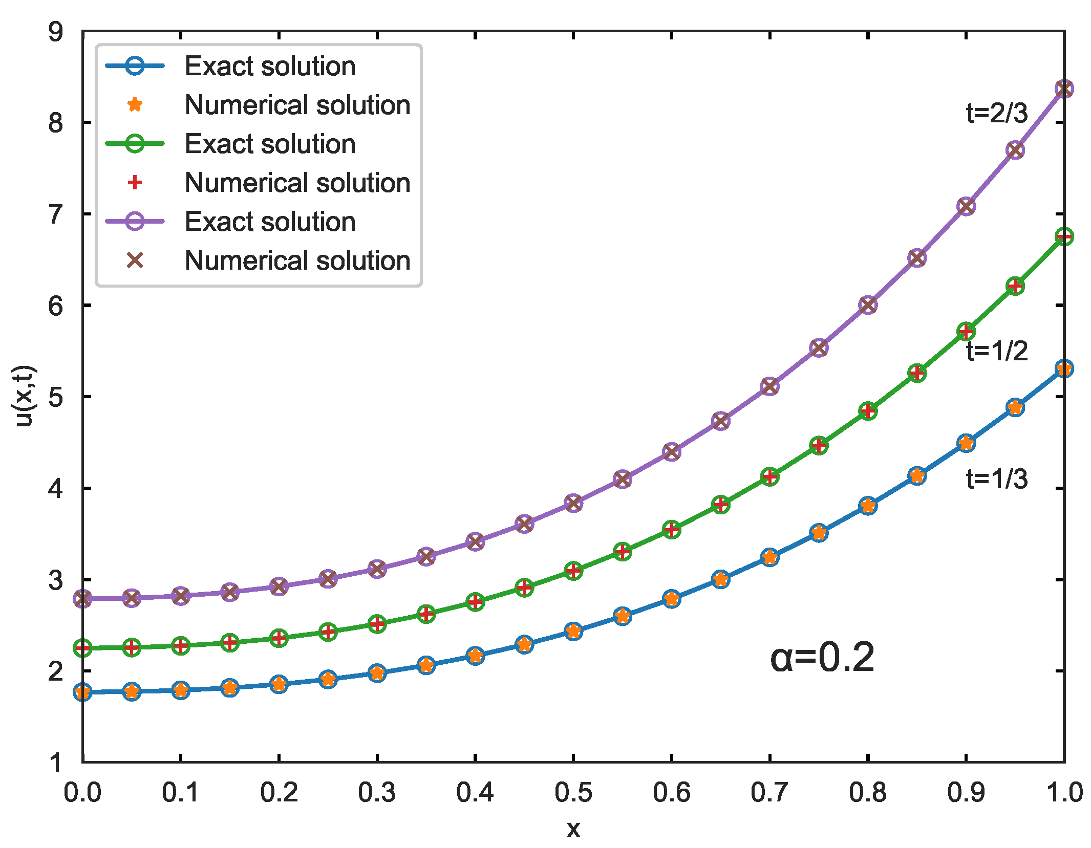
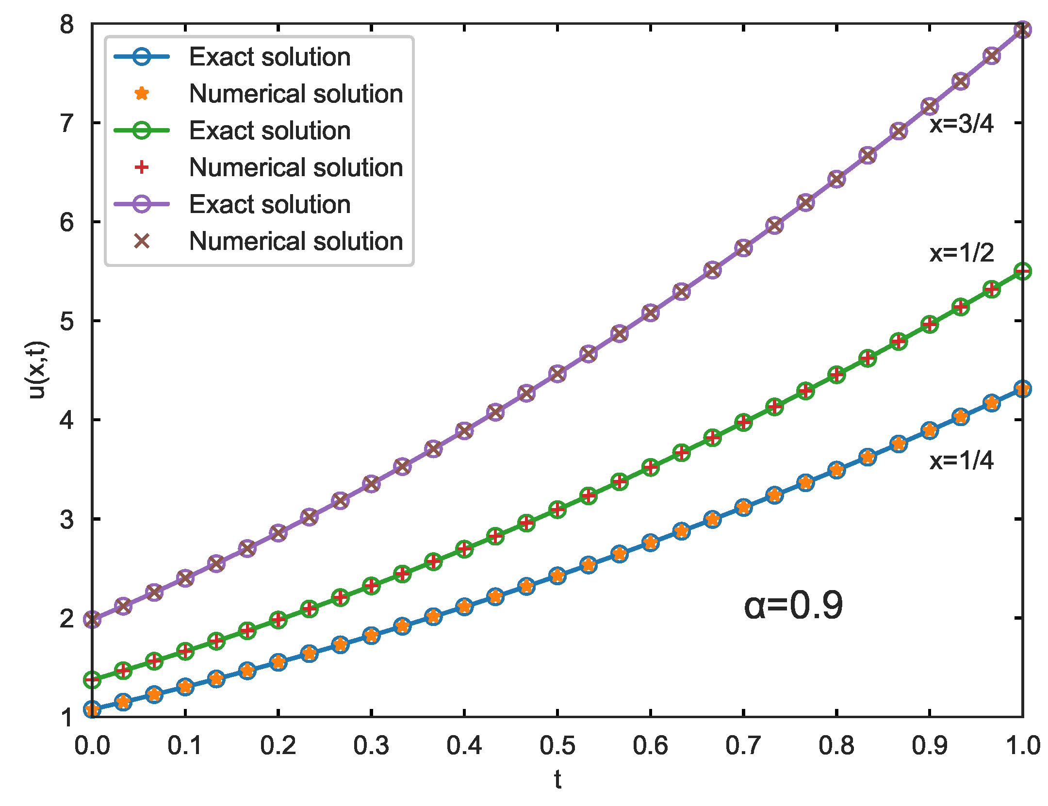
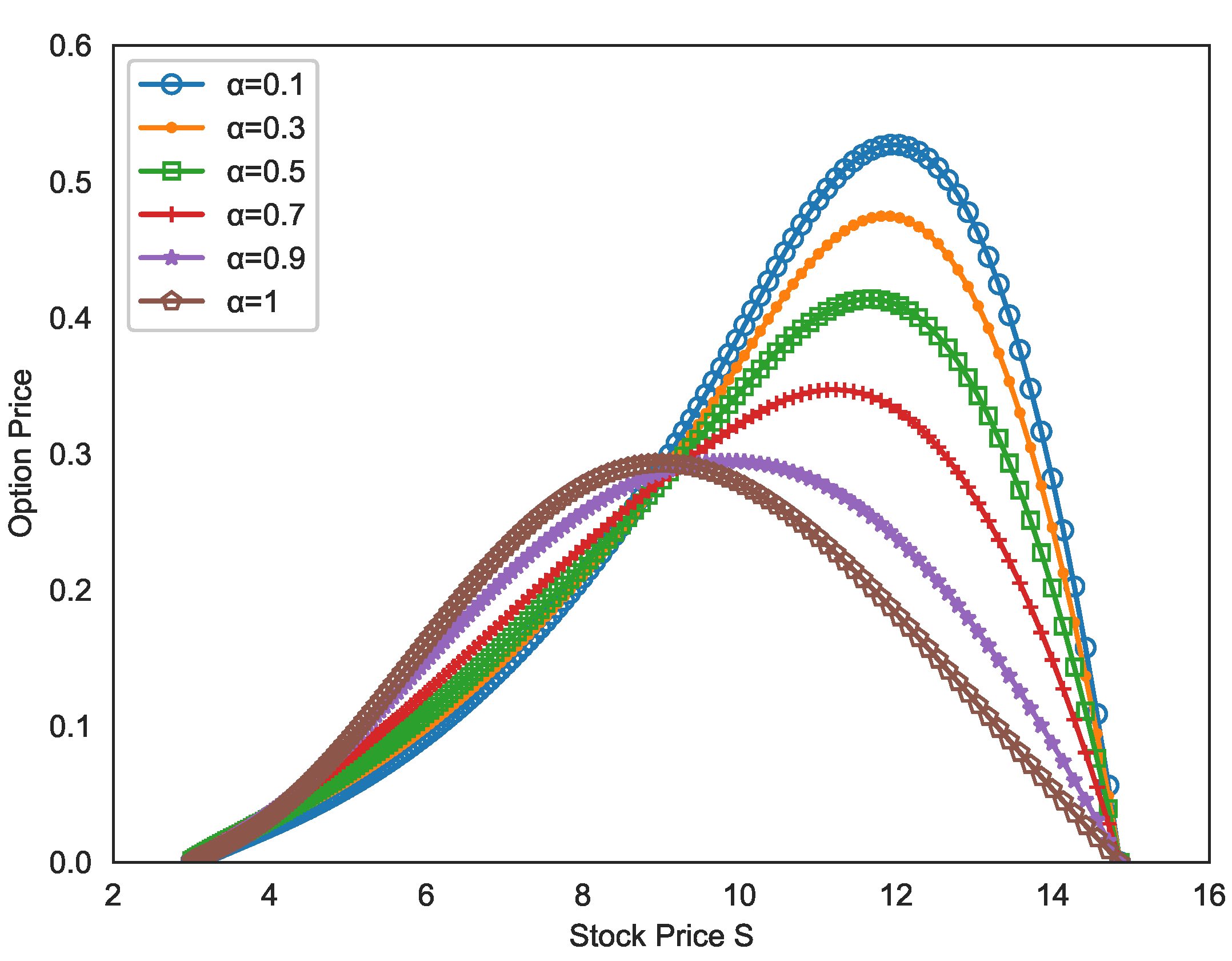
4. Numerical Examples

In this section, we present some numerical examples to verify the effectiveness and accuracy of the derived high-order numerical method.
Define Error
e ( Δ t , h ) = max 1 n N e n 2 = max 1 n N h j = 1 M 1 e j n 2 1 2 .
The convergence order of the derived high-order numerical method in time is calculated by
Order = log 2 e ( 2 Δ t , h ) e ( Δ t , h ) ,
and the convergence order of the derived high-order numerical method in space is calculated by
Order = log 2 e ( Δ t , 2 h ) e ( Δ t , h ) .
Example 1 
(known solution). Consider the following time-fractional advection–diffusion model [6]:
  0 C D t α u ( x , t ) = 2 u ( x , t ) x 2 0.5 u ( x , t ) x 0.5 u ( x , t ) + f ( x , t ) , ( x , t ) [ 0 , 1 ] × [ 0 , 1 ] , u ( x , 0 ) = 1 + x 2 + x 3 , x [ 0 , 1 ] , u ( 0 , t ) = ( 1 + t ) 2 , u ( 1 , t ) = 3 ( 1 + t ) 2 , t [ 0 , 1 ] ,
where
f ( x , t ) = 2 t 2 α Γ ( 3 α ) + 2 t 1 α Γ ( 2 α ) 1 + x 2 + x 3 ( 1 + t ) 2 ( 2 + 6 x ) 0.5 ( 2 x + 3 x 2 ) 0.5 1 + x 2 + x 3 .
The exact analytical solution is u ( x , t ) = ( 1 + t ) 2 ( 1 + x 2 + x 3 ) .
We solve the problem using the derived high-order numerical method (19)–(22). Table 1 shows the calculated errors and the corresponding convergence orders in time for different fractional derivative α = 0.3 , 0.5 , 0.7 and a fixed h = 1 / 1000 . From Table 1, we can obviously see that the convergence order in time is O ( Δ t 2 α ) , which is in agreement with the theoretical analysis.
Table 2 shows the calculated errors and the corresponding convergence orders in space for different fractional derivative α = 0.3 , 0.5 , 0.7 and a fixed Δ t = 1/100,000. From Table 2, one can see that the convergence order in space is O ( h 4 ) , which is in agreement with the theoretical analysis.
Table 3 shows the comparison of error and convergence order in space, calculated using the derived high-order numerical method (19)–(22) and previous research [6,18,19] when the fractional derivative α = 0.7 and Δ t = 1 / 100,000. From Table 3, one can see that the derived high-order numerical method (19)–(22) gains the same convergence order in space as [18,19], which is higher than [6]. Furthermore, all the above analyses demonstrate that our derived high-order numerical method (19)–(22) is effective.
Figure 1 illustrates the comparison between the exact solutions and the numerical solutions at t = 1 / 3 , 1 / 2 , 2 / 3 when α = 0.2 . Figure 2 illustrates the comparison between the exact solutions and the numerical solutions at x = 1 / 4 , 1 / 2 , 3 / 4 when α = 0.9 . From Figure 1 and Figure 2, one can obviously observe that the numerical solutions are remarkably consistent with the exact solutions, which indicates the efficiency of the derived high-order numerical method.
Example 2 
(unknown solution). Consider the following time-fractional Black–Scholes model, which describes the European double barrier knock-out call option [6,10]:
α V ( S , τ ) τ α + 1 2 σ 2 S 2 2 V ( S , τ ) S 2 + ( r D ) S V ( S , τ ) S r V ( S , τ ) = 0 , ( S , τ ) ( 3 , 15 ) × ( 0 , 1 ) , V ( S , T ) = max { S K , 0 } , V ( 3 , τ ) = 0 , V ( 15 , τ ) = 0 .
Here, the parameter values are taken to be the same as in reference [6,10]: σ = 0.45 , r = 0.03 , D = 0.01 , T = 1 , K = 10 . The double barrier knock-out call is obtained if the price of a knock-out call whose strike is within the two barriers is worked out; more details can be found in [10].
Since the exact analytical solution is not known, we solve this problem by the derived high-order numerical method (19)–(22) for different fractional derivative value. Numerical results are presented graphically.
Figure 3 illustrates the European double barrier knock-out call option prices for different time-fractional derivative α = 0.1 , 0.3 , 0.5 , 0.7 , 0.9 , 1 . From Figure 3, one can see that how the call option prices are affected by the strike price K and the time-fractional derivative α . Furthermore, we can conclude that the time-fractional Black–Scholes model can display more characteristics of the call option price changes than the classical Black–Scholes model ( α = 1 ) .

5. Conclusions

Due to the fact that the exact solution of the fractional partial differential equation is not easy to obtain, and can even be impossible, we have derived a new high-order numerical method based on a spatial compact exponential scheme for solving the time-fractional Black–Scholes model. Firstly, by means of the variable transformation technique, we convert the original time-fractional Black–Scholes equation into an equivalent time-fractional advection–diffusion reaction equation, then we construct a new high-order numerical method with ( 2 α ) accuracy in time and fourth-order accuracy in space based on spatial compact exponential scheme, which is different from the previous research [6,18,19]. We have rigorously discussed the uniqueness of solvability, and the unconditional stability and convergence of the derived high-order numerical method. Finally, two examples, whose exact solutions are known and unknown, are given to illustrate the efficiency of the derived high-order numerical method.

Author Contributions

Conceptualization, B.Y.; methodology, X.H. and B.Y.; software, X.H. and B.Y.; validation, X.H. and B.Y.; formal analysis, X.H. and B.Y.; investigation, X.H. and B.Y.; writing—original draft preparation, X.H. and B.Y.; writing—review and editing, X.H. and B.Y.; supervision, B.Y.; funding acquisition, B.Y. All authors have read and agreed to the published version of the manuscript.

Funding

This research was funded by Shandong Provincial Natural Science Foundation, China, grant number ZR2022MA021 and China Postdoctoral Science Foundation, Grant number 2018T110679.

Data Availability Statement

Data are contained within the article.

Acknowledgments

The authors thank the editors and the referees for their valuable comments and helpful suggestions.

Conflicts of Interest

The authors declare no conflicts of interest.

References

  1. Podlubny, I. Fractional Differential Equations; Academic Press: San Diego, CA, USA, 1999. [Google Scholar]
  2. Hilfer, R. Applications of Fractional Calculus in Physics; World Scientific: Singapore, 2000. [Google Scholar]
  3. Magin, R.L. Fractional Calculus in Bioengineering; Begell House Publishers: Danbury, CT, USA, 2006. [Google Scholar]
  4. Black, F.; Scholes, M. The pricing of options and corporate liabilities. J. Polit. Econ. 1973, 81, 637–654. [Google Scholar] [CrossRef]
  5. Merton, R.C. Theory of rational option pricing. Bell J. Econ. Manag. Sci. 1973, 4, 141–183. [Google Scholar] [CrossRef]
  6. Zhang, H.; Liu, F.; Turner, I.; Yang, Q. Numerical solution of the time fractional Black–Scholes model governing European options. Comput. Math. Appl. 2016, 69, 1772–1783. [Google Scholar] [CrossRef]
  7. Cartea, A.; del-Castillo-Negrete, D. Fractional diffusion models of option prices in markets with jumps. Physical A 2007, 374, 749–763. [Google Scholar] [CrossRef]
  8. Jumarie, G. Stock exchange fractional dynamics defined as fractional exponential growth driven by (usual) Gaussian white noise. Application to fractional Black–Scholes equations. Insurance Math. Econom. 2008, 42, 271–287. [Google Scholar] [CrossRef]
  9. Liang, J.R.; Wang, J.; Zhang, W.J.; Qiu, W.Y.; Ren, F.Y. The solutions to a bi-fractional black-scholes-merton differential equation. Int. J. Pure Appl. Math. 2010, 58, 99–112. [Google Scholar]
  10. Chen, W.; Xu, X.; Zhu, S. Analytically pricing double barrier options based on a time-fractional Black–Scholes equation. Comput. Math. Appl. 2015, 69, 1407–1419. [Google Scholar] [CrossRef]
  11. Zhang, H.M.; Zhang, M.C.; Liu, F.W.; Shen, M. Review of the fractional Black-Scholes equations and their solution techniques. Fractal Fract. 2024, 8, 101. [Google Scholar] [CrossRef]
  12. Liu, F.; Zhuang, P.; Liu, Q. Numerical Methods of Fractional Partial Differential Equations and Applications; Science Press: Beijing, China, 2015. [Google Scholar]
  13. Cai, M.; Li, C.P. Theory and Numerical Approximations of Fractional Integrals and Derivatives; Society for Industrial and Applied Mathematics: Philadelphia, PA, USA, 2019. [Google Scholar]
  14. Yu, B.; Jiang, X. Numerical Identification of the Fractional Derivatives in the Two-Dimensional Fractional Cable Equation. J. Sci. Comput. 2016, 68, 252–272. [Google Scholar] [CrossRef]
  15. Yu, B.; Jiang, X. Temperature prediction by a fractional heat conduction model for the bi-layered spherical tissue in the hyperthermia experiment. Int. J. Therm. Sci. 2019, 145, 105990. [Google Scholar] [CrossRef]
  16. Yu, B. High-order efficient numerical method for solving a generalized fractional Oldroyd-B fluid model. J. Appl. Math. Comput. 2021, 66, 749–768. [Google Scholar] [CrossRef]
  17. Yu, B. High-order compact finite difference method for the multi-term time fractional mixed diffusion and diffusion-wave equation. Math. Meth. Appl. Sci. 2021, 44, 6526–6539. [Google Scholar] [CrossRef]
  18. De Staelen, R.H.; Hendy, A.S. Numerically pricing double barrier options in a time-fractional Black-Scholes model. Comput. Math. Appl. 2017, 74, 1166–1175. [Google Scholar] [CrossRef]
  19. Roul, P.; Goura, V.M.K.P. A compact finite difference scheme for fractional Black-Scholes option pricing model. Appl. Numer. Math. 2021, 166, 40–60. [Google Scholar] [CrossRef]
  20. Roul, P. A high accuracy numerical method and its convergence for time-fractional Black-Scholes equation governing European options. Appl. Numer. Math. 2020, 151, 472–493. [Google Scholar] [CrossRef]
  21. An, X.Y.; Liu, F.W.; Zheng, M.L.; Anh, V.; Turner, I.W. A space-time spectral method for time-fractional Black-Scholes equation. Appl. Numer. Math. 2021, 165, 152–166. [Google Scholar] [CrossRef]
  22. Song, K.; Lyu, P. A high-order and fast scheme with variable time steps for the time-fractional Black-Scholes equation. Math. Meth. Appl. Sci. 2023, 46, 1990–2011. [Google Scholar] [CrossRef]
  23. Abdi, N.; Aminikhah, H.; Sheikhani, A.H.R. High-order compact finite difference schemes for the time-fractional Black-Scholes model governing European options. Chaos Solitons Fractals 2022, 162, 112423. [Google Scholar] [CrossRef]
  24. Taghipour, M.; Aminikhah, H. A spectral collocation method based on fractional Pell functions for solving time–fractional Black–Scholes option pricing model. Chaos Solitons Fractals 2022, 163, 112571. [Google Scholar] [CrossRef]
  25. Kaur, J.; Natesan, S. A novel numerical scheme for time-fractional Black-Scholes PDE governing European options in mathematical finance. Numer Algor. 2023, 94, 1519–1549. [Google Scholar] [CrossRef]
  26. Zhang, M.; Zheng, X. Numerical approximation to a variable-order time-fractional Black–Scholes model with applications in option pricing. Comput. Econ. 2023, 62, 1155–1175. [Google Scholar] [CrossRef]
  27. Kazmi, K. A second order numerical method for the time-fractional Black-Scholes European option pricing model. J. Comput. Appl. Math. 2023, 418, 114647. [Google Scholar] [CrossRef]
  28. Tian, Z.; Dai, S. High-order compact exponential finite difference methods for convection–diffusion type problems. J. Comput. Phys. 2007, 220, 952–974. [Google Scholar] [CrossRef]
  29. Tian, Z.; Yu, P. A high-order exponential scheme for solving 1D unsteady convection–diffusion equations. J. Comput. Appl. Math. 2011, 235, 2477–2491. [Google Scholar] [CrossRef]
  30. Sun, Z.; Wu, X. A fully discrete difference scheme for a diffusion-wave system. Appl. Numer. Math. 2006, 56, 193–209. [Google Scholar] [CrossRef]
Figure 1. Comparison between the exact solutions and the numerical solutions at t = 1 / 3 , 1 / 2 , 2 / 3 when α = 0.2 .
Fractalfract 08 00465 g001
Figure 2. Comparison between the exact solutions and the numerical solutions at x = 1 / 4 , 1 / 2 , 3 / 4 when α = 0.9 .
Fractalfract 08 00465 g002
Figure 3. European double barrier knock-out call option prices for different fractional derivative α .
Fractalfract 08 00465 g003
Table 1. Error and convergence order in time for different fractional derivative α .
α h Δ t ErrorOrder
0.3 1 / 1000 1 / 50 3.0904 × 10 5
1 / 100 9.5107 × 10 6 1.7002
1 / 200 2.8887 × 10 6 1.7191
1 / 400 8.8774 × 10 7 1.7022
0.5 1 / 1000 1 / 50 1.5922 × 10 4
1 / 100 5.6500 × 10 5 1.4947
1 / 200 1.9622 × 10 5 1.5258
1 / 400 6.9500 × 10 6 1.4974
0.7 1 / 1000 1 / 50 5.0784 × 10 4
1 / 100 2.0581 × 10 4 1.3031
1 / 200 8.2092 × 10 5 1.3260
1 / 400 3.3446 × 10 5 1.2954
Table 2. Error and convergence order in space for different fractional derivative α .
α Δ t hErrorOrder
0.3 1 / 100,000 1 / 3 3.4538 × 10 3
1 / 6 2.2358 × 10 4 3.9493
1 / 12 1.4382 × 10 5 3.9585
1 / 24 8.9254 × 10 7 4.0102
0.5 1 / 100,000 1 / 3 3.4295 × 10 3
1 / 6 2.2965 × 10 4 3.9005
1 / 12 1.5270 × 10 5 3.9107
1 / 24 9.6455 × 10 7 3.9847
0.7 1/100,000 1 / 3 7.8382 × 10 3
1 / 6 4.5642 × 10 4 4.1021
1 / 12 2.6758 × 10 5 4.0923
1 / 24 1.6697 × 10 6 4.0023
Table 3. Comparison of error and convergence order in space with [6,18,19] when α = 0.7 and Δ t = 1 / 100,000.
hError [6]Order [6]Error [18,19]Order [18,19]ErrorOrder
1 / 3 1.7089 × 10 2 3.9506 × 10 2 7.8382 × 10 3
1 / 6 4.3376 × 10 3 1.9781 2.4873 × 10 3 3.9894 4.5642 × 10 4 4.1021
1 / 12 1.0866 × 10 3 1.9971 1.5602 × 10 4 3.9948 2.6758 × 10 5 4.0923
1 / 24 2.7142 × 10 4 2.0012 9.6117 × 10 6 4.0208 1.6697 × 10 6 4.0023
Disclaimer/Publisher’s Note: The statements, opinions and data contained in all publications are solely those of the individual author(s) and contributor(s) and not of MDPI and/or the editor(s). MDPI and/or the editor(s) disclaim responsibility for any injury to people or property resulting from any ideas, methods, instructions or products referred to in the content.

