
A Fast Second-Order ADI Finite Difference Scheme for the Two-Dimensional Time-Fractional Cattaneo Equation with Spatially Variable Coefficients


Abstract
1. Introduction
2. Derivation of the Difference Scheme
3. The Derivation of the Fast ADI Difference Scheme
- First, the intermediate variables are obtained by computing the system
- Then, we obtain the numerical solution by solving
4. Stability and Error Estimate
5. Numerical Examples
- (a)
- and ;
- (b)
- ;
- (c)
- ;
- (d)
- and .
6. Conclusions
Author Contributions
Funding
Data Availability Statement
Acknowledgments
Conflicts of Interest
References
- Compte, A.; Metzler, R. The generalized Cattaneo equation for the description of anomalous transport processes. J. Phys. Math. Gen. 1997, 30, 7277–7289. [Google Scholar] [CrossRef]
- Ghazizadeh, H.; Maerefat, M.; Azimi, A. Explicit and implicit finite difference schemes for fractional Cattaneo equation. J. Comput. Phys. 2010, 229, 7042–7057. [Google Scholar] [CrossRef]
- Ferrillo, F.; Spigler, R.; Concezzi, M. Comparing Cattaneo and Fractional Derivative Models for Heat Transfer Processes. SIAM J. Appl. Math. 2018, 78, 1450–1469. [Google Scholar] [CrossRef]
- Zorica, D.; Cvetićanin, S.M. Fractional telegrapher’s equation as a consequence of Cattaneo’s heat conduction law generalization. Theor. Appl. Mech. 2018, 45, 35–51. [Google Scholar] [CrossRef]
- Chen, A.; Nong, L. Efficient Galerkin finite element methods for a time-fractional Cattaneo equation. Adv. Differ. Equ. 2020, 2020, 545. [Google Scholar] [CrossRef]
- Nong, L.; Yi, Q.; Cao, J.; Chen, A. Fast Compact Difference Scheme for Solving the Two-Dimensional Time-Fractional Cattaneo Equation. Fractal Fract. 2022, 6, 438. [Google Scholar] [CrossRef]
- Cui, M. Compact exponential scheme for the time fractional convection–diffusion reaction equation with variable coefficients. J. Comput. Phys. 2015, 280, 143–163. [Google Scholar] [CrossRef]
- Lin, X.l.; Ng, M.K.; Sun, H.W. Crank–Nicolson Alternative Direction Implicit Method for Space-Fractional Diffusion Equations with Nonseparable Coefficients. SIAM J. Numer. Anal. 2019, 57, 997–1019. [Google Scholar] [CrossRef]
- Cheng, X.; Qin, H.; Zhang, J. A compact ADI scheme for two-dimensional fractional sub-diffusion equation with Neumann boundary condition. Appl. Numer. Math. 2020, 156, 50–62. [Google Scholar] [CrossRef]
- Zhu, C.; Zhang, B.; Fu, H.; Liu, J. Efficient second-order ADI difference schemes for three-dimensional Riesz space-fractional diffusion equations. Comput. Math. Appl. 2021, 98, 24–39. [Google Scholar] [CrossRef]
- Qiao, L.; Qiu, W.; Xu, D. Error analysis of fast L1 ADI finite difference/compact difference schemes for the fractional telegraph equation in three dimensions. Math. Comput. Simul. 2023, 205, 205–231. [Google Scholar] [CrossRef]
- Lyu, P.; Vong, S. A weighted ADI scheme with variable time steps for diffusion-wave equations. Calcolo 2023, 60, 49. [Google Scholar] [CrossRef]
- Ren, J.; Gao, G.H. Efficient and stable numerical methods for the two-dimensional fractional Cattaneo equation. Numer. Algorithms 2015, 69, 795–818. [Google Scholar] [CrossRef]
- Zhao, X.; Sun, Z.Z. Compact Crank–Nicolson Schemes for a Class of Fractional Cattaneo Equation in Inhomogeneous Medium. J. Sci. Comput. 2015, 62, 747–771. [Google Scholar] [CrossRef]
- Chen, A.; Li, C. An alternating direction Galerkin method for a time-fractional partial differential equation with damping in two space dimensions. Adv. Differ. Equ. 2017, 2017, 356. [Google Scholar] [CrossRef]
- Zhou, Y.; Li, C.; Stynes, M. A fast second-order predictor-corrector method for a nonlinear time-fractional Benjamin-Bona-Mahony-Burgers equation. Numer. Algorithms 2024, 95, 693–720. [Google Scholar] [CrossRef]
- Bu, W.; Yang, H.; Tang, Y. Two fast numerical methods for a generalized Oldroyd-B fluid model. Commun. Nonlinear Sci. Numer. Simul. 2023, 117, 106963. [Google Scholar] [CrossRef]
- Ming, W.; Li, M.; Lu, Y.; Li, M. A fast linearized Galerkin finite element method for the nonlinear multi-term time fractional wave equation. Comput. Math. Appl. 2024, 157, 27–48. [Google Scholar] [CrossRef]
- Wang, Y.M.; Zheng, Z.Y. A second-order L2-1σ Crank-Nicolson difference method for two-dimensional time-fractional wave equations with variable coefficients. Comput. Math. Appl. 2022, 118, 183–207. [Google Scholar] [CrossRef]
- Li, X.; Liao, H.l.; Zhang, L. A second-order fast compact scheme with unequal time-steps for subdiffusion problems. Numer. Algorithms 2021, 86, 1011–1039. [Google Scholar] [CrossRef]
- Yan, Y.; Sun, Z.Z.; Zhang, J. Fast Evaluation of the Caputo Fractional Derivative and its Applications to Fractional Diffusion Equations: A Second-Order Scheme. Commun. Comput. Phys. 2017, 22, 1028–1048. [Google Scholar] [CrossRef]
- Sun, H.; Sun, Z.; Gao, G. Some temporal second order difference schemes for fractional wave equations. Numer. Methods Partial. Differ. Equ. 2016, 32, 970–1001. [Google Scholar] [CrossRef]
- Du, R.l.; Sun, Z.z.; Wang, H. Temporal Second-Order Finite Difference Schemes for Variable-Order Time-Fractional Wave Equations. SIAM J. Numer. Anal. 2022, 60, 104–132. [Google Scholar] [CrossRef]
- Lv, C.; Xu, C. Error Analysis of a High Order Method for Time-Fractional Diffusion Equations. SIAM J. Sci. Comput. 2016, 38, A2699–A2724. [Google Scholar] [CrossRef]
- Wang, Y.M.; Ren, L. A high-order L2-compact difference method for Caputo-type time-fractional sub-diffusion equations with variable coefficients. Appl. Math. Comput. 2019, 342, 71–93. [Google Scholar] [CrossRef]
- Xie, J.; Zhang, Z. The high-order multistep ADI solver for two-dimensional nonlinear delayed reaction–diffusion equations with variable coefficients. Comput. Math. Appl. 2018, 75, 3558–3570. [Google Scholar] [CrossRef]
- Sun, Z.z. Numerical Methods for Partial Differential Equations, 3rd ed.; Science Press: Beijing, China, 2022; p. 71. [Google Scholar]

| Cases | |||||||
|---|---|---|---|---|---|---|---|
| Error | Rate | Error | Rate | Error | Rate | ||
| (a) | 4 | 3.88 × | - | 2.88 × | - | 2.10 × | - |
| 8 | 1.27 × | 1.61 | 7.16 × | 2.01 | 4.69 × | 2.16 | |
| 16 | 3.35 × | 1.92 | 1.53 × | 2.23 | 1.03 × | 2.19 | |
| 32 | 8.22 × | 2.03 | 3.14 × | 2.28 | 2.32 × | 2.15 | |
| (b) | 4 | 6.05 × | - | 4.47 × | - | 2.95 × | - |
| 8 | 2.27 × | 1.42 | 1.20 × | 1.90 | 6.27 × | 2.23 | |
| 16 | 6.31 × | 1.85 | 2.55 × | 2.23 | 1.27 × | 2.30 | |
| 32 | 1.58 × | 2.00 | 5.14 × | 2.31 | 2.70 × | 2.24 | |
| (c) | 4 | 2.95 × | - | 2.24 × | - | 1.74 × | - |
| 8 | 9.22 × | 1.68 | 5.46 × | 2.04 | 3.99 × | 2.13 | |
| 16 | 2.40 × | 1.94 | 1.17 × | 2.22 | 8.98 × | 2.15 | |
| 32 | 5.85 × | 2.04 | 2.42 × | 2.27 | 2.07 × | 2.12 | |
| (d) | 4 | 4.48 × | - | 3.29 × | - | 2.32 × | - |
| 8 | 1.50 × | 1.58 | 8.28 × | 1.99 | 5.12 × | 2.18 | |
| 16 | 4.00 × | 1.91 | 1.77 × | 2.23 | 1.11 × | 2.21 | |
| 32 | 9.93 × | 2.01 | 3.83 × | 2.21 | 2.76 × | 2.00 | |
| Cases | M | ||||||
|---|---|---|---|---|---|---|---|
| Error | Rate | Error | Rate | Error | Rate | ||
| (a) | 4 | 7.93 × | - | 7.65 × | - | 7.01 × | - |
| 8 | 2.00 × | 1.99 | 1.93 × | 1.98 | 1.76 × | 1.99 | |
| 16 | 5.02 × | 2.00 | 4.85 × | 1.99 | 4.41 × | 2.00 | |
| 32 | 1.26 × | 2.00 | 1.21 × | 2.00 | 1.10 × | 2.00 | |
| (b) | 4 | 8.19 × | - | 8.01 × | - | 7.22 × | - |
| 8 | 2.06 × | 1.99 | 2.02 × | 1.99 | 1.85 × | 1.96 | |
| 16 | 5.17 × | 2.00 | 5.06 × | 2.00 | 4.68 × | 1.99 | |
| 32 | 1.29 × | 2.00 | 1.27 × | 2.00 | 1.17 × | 2.00 | |
| (c) | 4 | 7.74 × | - | 7.38 × | - | 7.12 × | - |
| 8 | 1.94 × | 2.00 | 1.85 × | 2.00 | 1.78 × | 2.00 | |
| 16 | 4.86 × | 2.00 | 4.64 × | 2.00 | 4.45 × | 2.00 | |
| 32 | 1.21 × | 2.00 | 1.16 × | 2.00 | 1.11 × | 2.00 | |
| (d) | 4 | 8.15 × | - | 7.90 × | - | 7.34 × | - |
| 8 | 2.03 × | 2.00 | 1.97 × | 2.00 | 1.83 × | 2.01 | |
| 16 | 5.09 × | 2.00 | 4.94 × | 2.00 | 4.57 × | 2.00 | |
| 32 | 1.28 × | 1.99 | 1.24 × | 1.99 | 1.15 × | 2.00 | |
| Cases | |||||||
|---|---|---|---|---|---|---|---|
| Error | Rate | Error | Rate | Error | Rate | ||
| (a) | 4 | 1.22 × | - | 1.85 × | - | 2.72 × | - |
| 8 | 6.31 × | 0.96 | 4.43 × | 2.06 | 7.70 × | 1.82 | |
| 16 | 3.80 × | 0.73 | 1.77 × | 1.33 | 1.68 × | 2.20 | |
| 32 | 2.38 × | 0.67 | 8.58 × | 1.04 | 3.35 × | 2.32 | |
| (b) | 4 | 1.69 × | - | 3.05 × | - | 4.19 × | - |
| 8 | 5.94 × | 1.51 | 7.69 × | 1.99 | 1.31 × | 1.67 | |
| 16 | 3.28 × | 0.85 | 1.56 × | 2.30 | 2.95 × | 2.15 | |
| 32 | 2.15 × | 0.61 | 7.62 × | 1.04 | 5.85 × | 2.33 | |
| (c) | 4 | 1.22 × | - | 1.42 × | - | 2.15 × | - |
| 8 | 6.62 × | 0.88 | 3.81 × | 1.90 | 5.85 × | 1.88 | |
| 16 | 4.17 × | 0.67 | 1.89 × | 1.01 | 1.27 × | 2.20 | |
| 32 | 2.58 × | 0.69 | 9.15 × | 1.04 | 3.58 × | 1.83 | |
| (d) | 4 | 1.25 × | - | 2.15 × | - | 3.11 × | - |
| 8 | 6.15 × | 1.02 | 5.19 × | 2.05 | 8.97 × | 1.79 | |
| 16 | 3.58 × | 0.78 | 1.70 × | 1.61 | 1.96 × | 2.20 | |
| 32 | 2.32 × | 0.63 | 8.33 × | 1.03 | 4.05 × | 2.27 | |
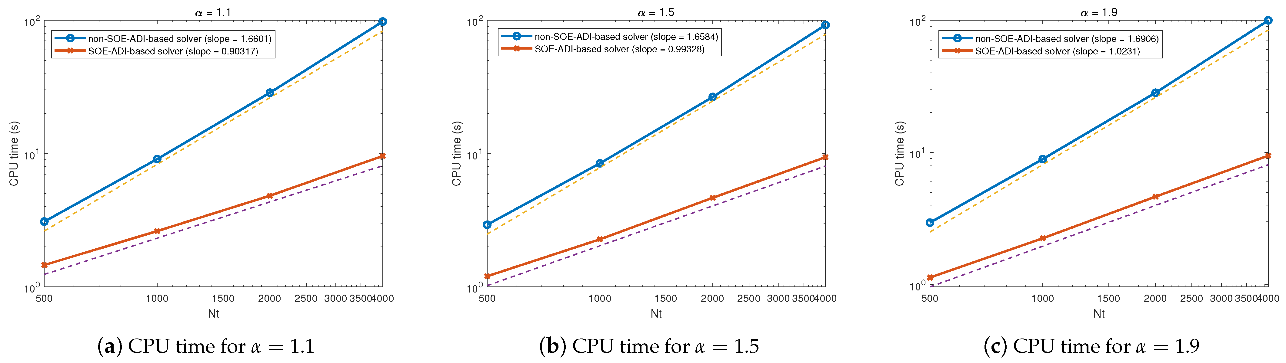
| Scheme | |||||||||
|---|---|---|---|---|---|---|---|---|---|
| Error | CPU (s) | Error | CPU (s) | Error | CPU (s) | Error | CPU (s) | ||
| 1.1 | (28) | 3.1413 × | 3.09 | 3.1405 × | 9.09 | 3.1402 × | 28.60 | 3.1402 × | 97.70 |
| (12) | 3.1159 × | 1.46 | 3.1344 × | 2.62 | 3.1388 × | 4.83 | 3.1398 × | 9.59 | |
| 1.5 | (28) | 3.0285 × | 2.93 | 3.0320 × | 8.45 | 3.0329 × | 26.58 | 3.0331 × | 92.12 |
| (12) | 3.0265 × | 1.20 | 3.0317 × | 2.27 | 3.0328 × | 4.66 | 3.0331 × | 9.39 | |
| 1.9 | (28) | 2.7571 × | 2.95 | 2.7576 × | 8.91 | 2.7577 × | 28.30 | 2.7577 × | 99.73 |
| (12) | 2.7571 × | 1.13 | 2.7576 × | 2.25 | 2.7577 × | 4.63 | 2.7577 × | 9.46 | |
Disclaimer/Publisher’s Note: The statements, opinions and data contained in all publications are solely those of the individual author(s) and contributor(s) and not of MDPI and/or the editor(s). MDPI and/or the editor(s) disclaim responsibility for any injury to people or property resulting from any ideas, methods, instructions or products referred to in the content. |
© 2024 by the authors. Licensee MDPI, Basel, Switzerland. This article is an open access article distributed under the terms and conditions of the Creative Commons Attribution (CC BY) license (https://creativecommons.org/licenses/by/4.0/).
Share and Cite
Nong, L.; Yi, Q.; Chen, A. A Fast Second-Order ADI Finite Difference Scheme for the Two-Dimensional Time-Fractional Cattaneo Equation with Spatially Variable Coefficients. Fractal Fract. 2024, 8, 453. https://doi.org/10.3390/fractalfract8080453
Nong L, Yi Q, Chen A. A Fast Second-Order ADI Finite Difference Scheme for the Two-Dimensional Time-Fractional Cattaneo Equation with Spatially Variable Coefficients. Fractal and Fractional. 2024; 8(8):453. https://doi.org/10.3390/fractalfract8080453
Chicago/Turabian StyleNong, Lijuan, Qian Yi, and An Chen. 2024. "A Fast Second-Order ADI Finite Difference Scheme for the Two-Dimensional Time-Fractional Cattaneo Equation with Spatially Variable Coefficients" Fractal and Fractional 8, no. 8: 453. https://doi.org/10.3390/fractalfract8080453
APA StyleNong, L., Yi, Q., & Chen, A. (2024). A Fast Second-Order ADI Finite Difference Scheme for the Two-Dimensional Time-Fractional Cattaneo Equation with Spatially Variable Coefficients. Fractal and Fractional, 8(8), 453. https://doi.org/10.3390/fractalfract8080453