Adaptive Morphing Activation Function for Neural Networks

Abstract

A novel morphing activation function is proposed, motivated by the wavelet theory and the use of wavelets as activation functions. Morphing refers to the gradual change of shape to mimic several apparently unrelated activation functions. The shape is controlled by the fractional order derivative, which is a trainable parameter to be optimized in the neural network learning process. Given the morphing activation function, and taking only integer-order derivatives, efficient piecewise polynomial versions of several existing activation functions are obtained. Experiments show that the performance of polynomial versions PolySigmoid, PolySoftplus, PolyGeLU, PolySwish, and PolyMish is similar or better than their counterparts Sigmoid, Softplus, GeLU, Swish, and Mish. Furthermore, it is possible to learn the best shape from the data by optimizing the fractional-order derivative with gradient descent algorithms, leading to the study of a more general formula based on fractional calculus to build and adapt activation functions with properties useful in machine learning.

1. Introduction

Since the seminal work of McCulloch and Pitts on the neural model [1] and Rosenblatt on perceptrons [2], activation functions have been a topic of interest in the context of artificial neural networks. In particular, given the singularity of the Heaviside function, derivable functions such as Sigmoid or tanh were introduced as activation functions [3]. Later, for deep learning, more activation functions were proposed to solve new challenges such as the gradient vanishing problem [4,5], where ReLU [6] plays an important role to the point of being considered the state of the art. Given the success of ReLU, more variants have been proposed, including Leaky ReLU [7], ELU [8], GeLU [9], Swish [10], and Mish [11], among others.

Two relevant concepts that have been considered to improve the results of neural networks are (i) activation functions with adaptive parameters and (ii) activation functions with fractional derivative, or even a combination of these, as in this paper. Certainly, this work is not a pioneer in introducing these concepts, and the papers [12,13,14,15,16,17] are evidence of this. In addition to the previous cited works, as justification and motivation to continue with this research of applying fractional derivatives to activation functions, the research of [18,19] was carried out, where fractional gradients were applied successfully to the backpropagation algorithm to improve the performance of the gradient descent algorithms available in Tensorflow and PyTorch. In such a case, the formula for updating the synaptic weights requires the derivative of the activation function and it involves the factor $D_x^{\nu }x={\displaystyle \frac{x^{1-\nu }}{\mathsf{\Gamma }(2-\nu )}}$, which reduces to 1 in the case of $\nu =1$, i.e., the first derivative of x with respect to x is 1, and makes it possible for it to be extended from integer to fractional orders. Furthermore, the experiments support the idea that fractional optimizers improve their integer-order versions.

Regarding activation functions with adaptive parameters, they can be trained through the learning process and are therefore called trainable or learnable, since the adaptation is obtained from the training data. Indeed, to improve the accuracy of neural networks, adaptive activation functions such as SPLASH or APTx have been studied. On the one hand, SPLASH is a class of learnable piecewise linear activation functions with parameterization to approximate non-linear functions [20]. On the other hand, APTx is similar to Mish but is intended to be more efficient to compute [21]. Other related works study ReLU variants, such as FELU [22], SELU, MPELU, and DELU [23], with parameters that consider non-zero values for the negative plane to solve the “Dying ReLU” phenomenon that stops learning [24]. Specifically, DELU considers three parameters, $\alpha ,\beta ,z_c\ge 0$, to be determined, and special cases are ELU ($\alpha =\beta =1,z_c=0$) and ReLU ($z_c=0,\beta \to \infty$). The Shape Autotuning Activation Function (SAAF) was proposed to simultaneously overcome three weaknesses of ReLU related to non-zero mean, negative missing (zero values), and unbounded output [25]. SAAF is a smooth function like Sigmoid and tanh, and piecewise like ReLU, but avoids some of their deficiencies by adjusting a pair of independent trainable parameters, $\alpha$ and $\beta$, to capture negative information and provide a near-zero mean output, which leads to better generalization and learning speed, as well as a bounded output. In [26], three variants of tanh, tanhSoft1, tanhSoft2, and tanhSoft3, are presented as trainable variants depending of $\alpha ,\beta$, and $\delta$ parameters that are used to control the slope of the curve on both positive and negative axes. Also, TanhLU is proposed in [26] as a combination of the tanh and a linear unit. All these works are examples of the effort to build and generalize some activation functions that, in addition to inheriting good properties from the original, provide flexibility with parameters to acquire useful properties for machine learning, such as control of overfitting or stop learning.

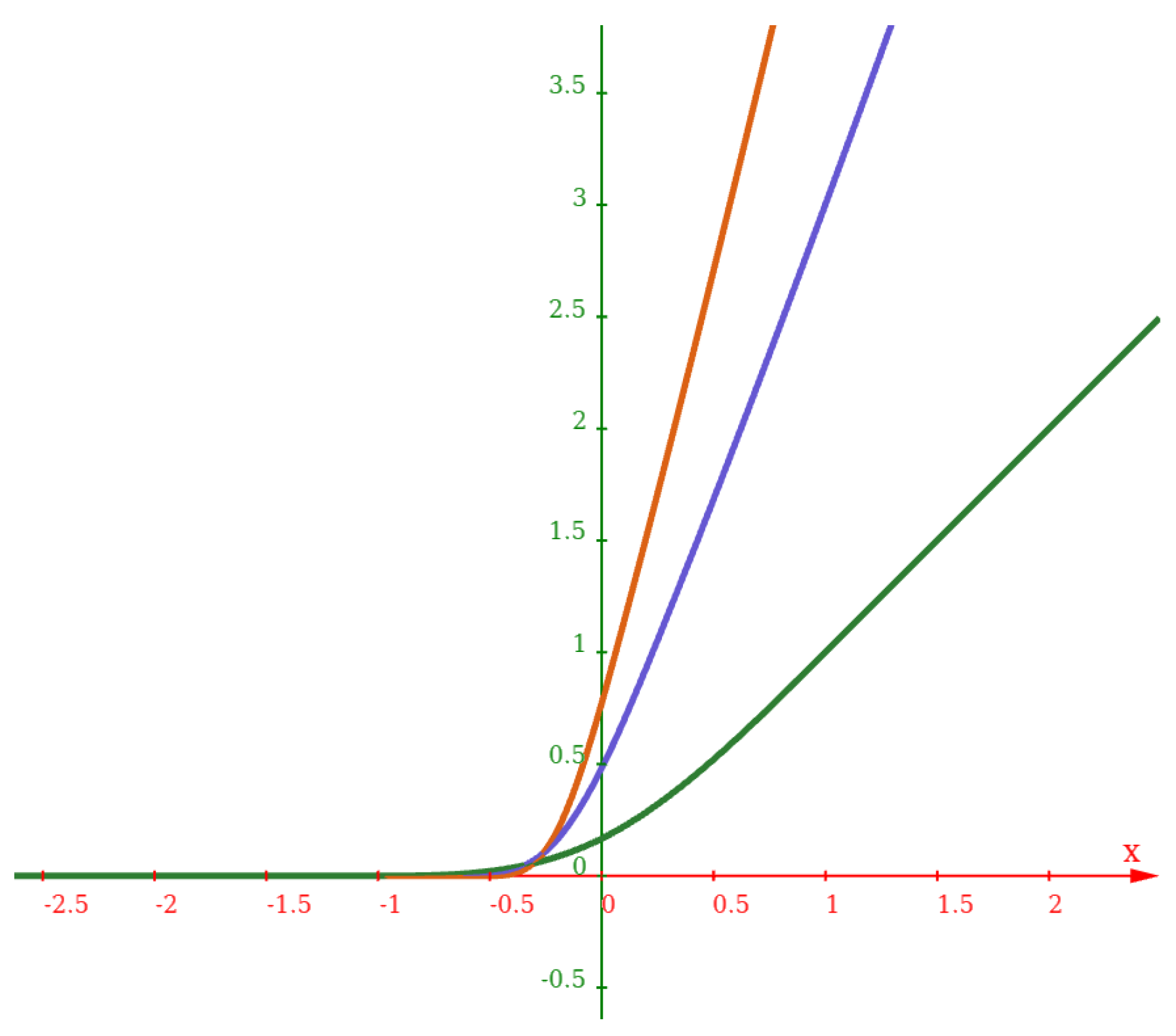
The other relevant topic considered in activation functions is the fractional derivative. The theoretical basis to extend the activation function derivative from integer to fractional order is the fractional calculus theory [27,28] that generalizes the integer operators: integration and differentiation. These two operators are combined in a single concept of fractional derivative once the integration is conceived as an antiderivative; thus, the orders are positive for derivatives and negative for antiderivatives so that, when added, the result is a real number, positive, negative, or zero. 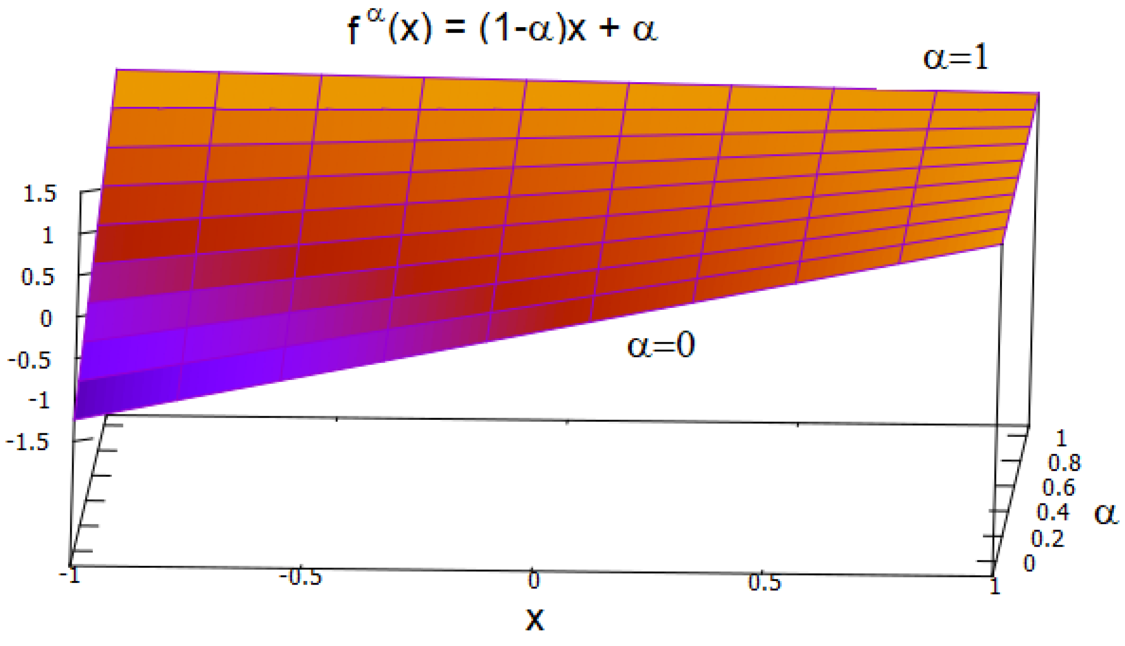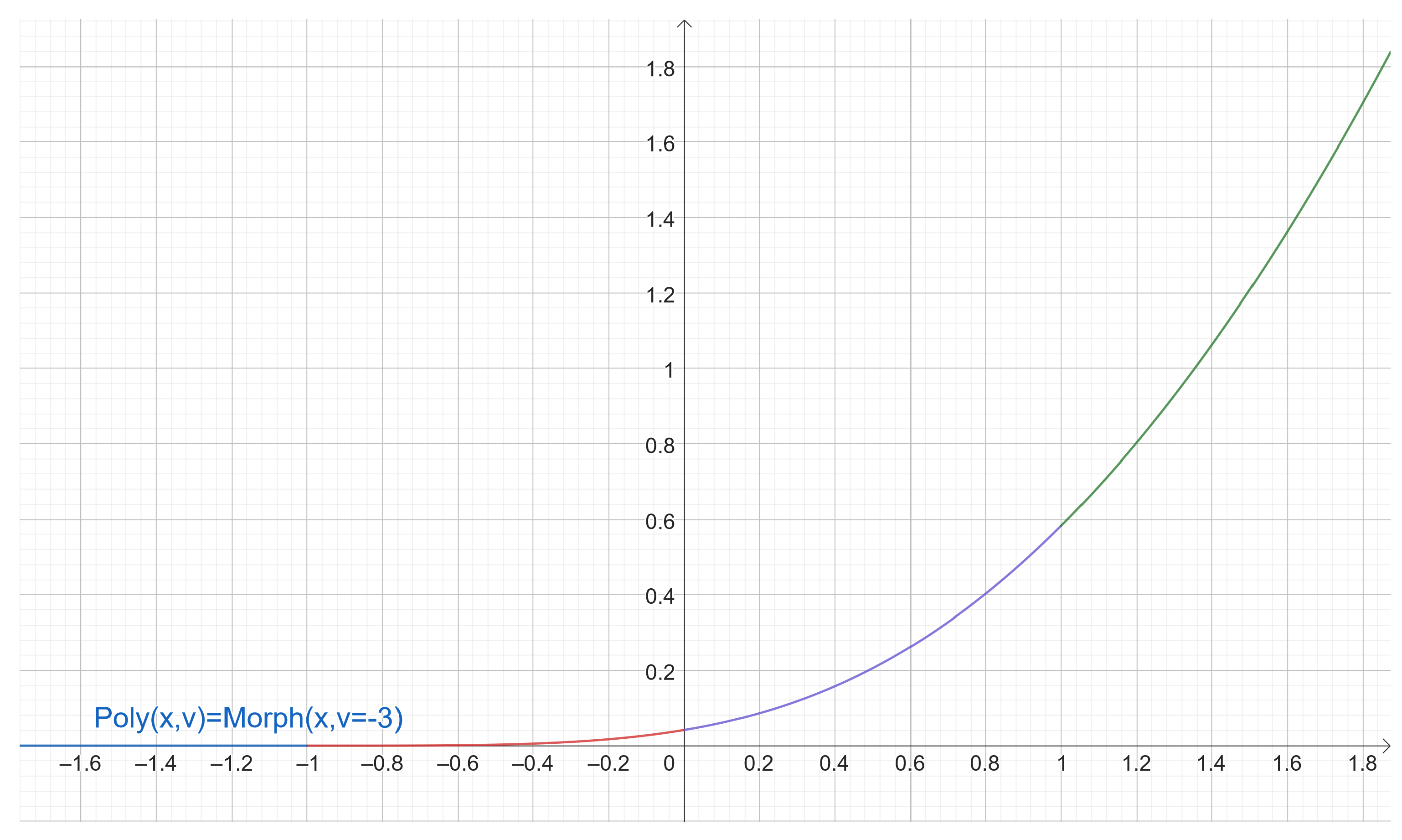Historically, instead of “real”, it is referred to as “fractional”, maybe because, in a letter, L’Hopital asked Leibniz about the order ${\displaystyle \frac{1}{2}}$ [29]. An intuitive approach comes from the interpolation between two functions. Let $f\left(x\right)=x$ and its first derivative $f^1\left(x\right)=1$; then, it is possible to build a “fractional” version with both of them. For $\alpha \in [0,1]$, we obtain $f^{\alpha }\left(x\right)=(1-\alpha )f\left(x\right)+\alpha f^1\left(x\right)=(1-\alpha )x+\alpha$. Now, if $\alpha =0$, there is no derivative, and $f^{\alpha }\left(x\right)$ is equal to x. However, if $\alpha =1$, then $f^{\alpha }\left(x\right)$ is equal to 1, meaning the first derivative of x. For “fractional” values, i.e., $0<x<1$, it corresponds to a line with gradient (slope) $1-\alpha$. 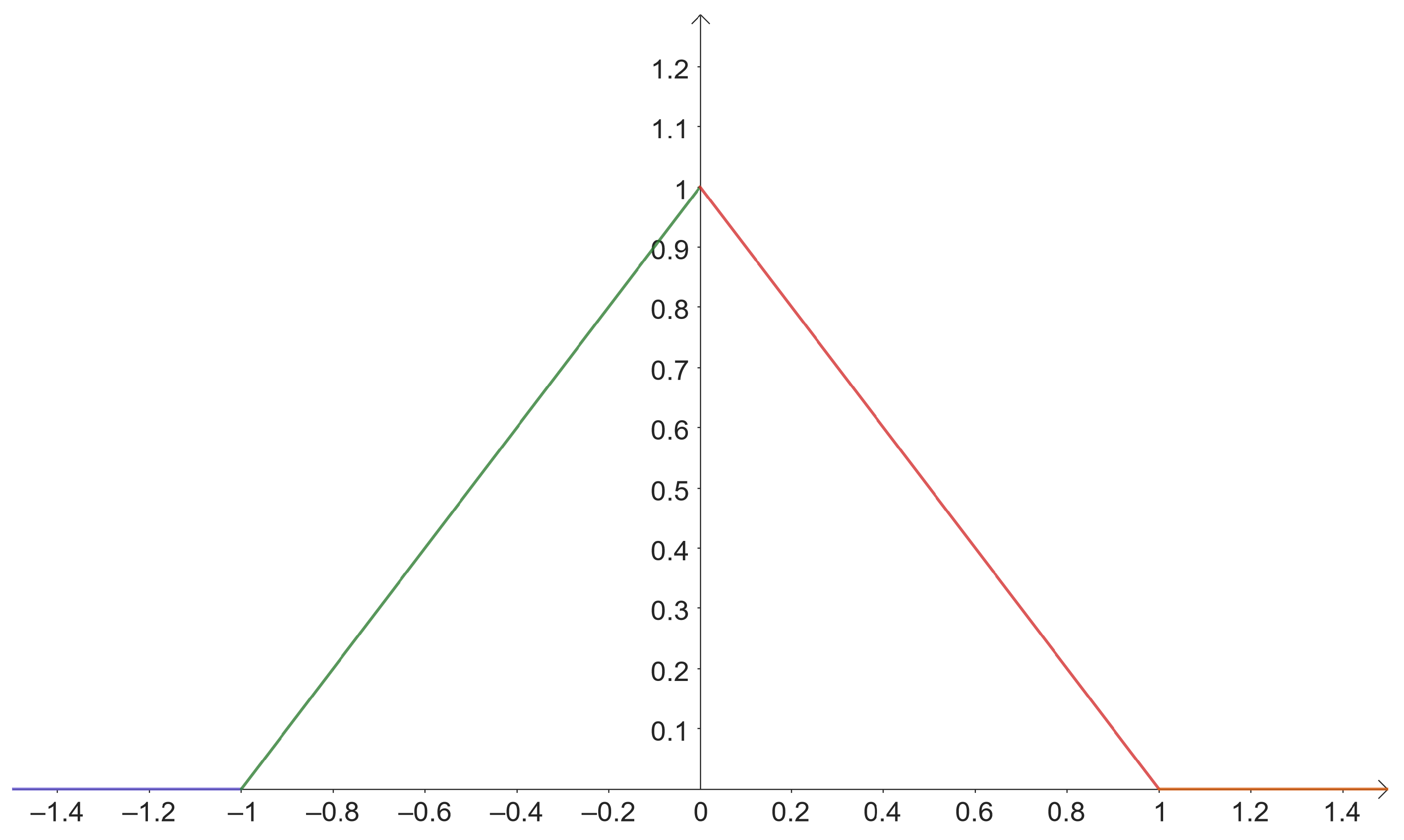So, it offers a mechanism to control the gradient, which could be useful in backpropagation algorithms [18,19] by considering that $f\left(x\right)$ could represent a more sophisticated activation function. It is illustrated in Figure 1, where there is a line with unitary slope for $\alpha =0$ and a horizontal line for $\alpha =1$. This $3D$ graph represents all lines with slopes in the interval $[0,1]$.

Effectively, fractional gradient optimizers [18,19] and fractional activation functions have been proposed based on fractional calculus concepts, as a generalization to the classic integer-order operators. For example, ref. [13] combines fractional derivatives on the activation functions and a fractional gradient descent backpropagation algorithm for perceptrons where, instead of choosing the first derivative, the fractional derivative of the activation function is applied. The experiments support the idea that the models that involve fractional derivatives are more accurate than the integer-order models. The fractional approach allows us to obtain the memory and hereditary properties of the processes described by the data, since it is a property of the fractional calculus operators [27,28,30]. This is possible because the derivative focuses on a point, but the integral operator covers (observes) a neighborhood (integration interval) around a point of interest. A more extensive study of the interpretation of the fractional derivative can be reviewed in [31], where one can find an analogy that was previously described from a physical point of view, specifically concerning the concept of divergence, which measures how much the vector field behaves like a source (positive divergence) or a sink (negative divergence).

In [17], fractional sigmoid activation functions and Fractional Rectified Linear Units (FReLUs) are proposed, and the order of the derivative of linear fractional activation functions is optimized in [15] to give a place to Fractional Adaptive Linear Units (FALUs).

Another possibility to apply fractional derivatives beyond the activation functions is to modify the standard loss functions, such as the Mean Squared Error (MSE), which involves a power of two, which can be modified to a fractional FMSE if it is multiplied by ${\displaystyle \frac{a}{2}}$ [12]. When the fractional order $a=2$, FSME is equivalent to MSE, but when a is not an integer, FMSE identifies more complex relationships between the input and the output. A similar approach can be used with the Cross-Entropy Loss function, to obtain a Fractional Cross-Entropy Loss function. However, the authors of [12] report that the fractional order a must be adjusted by trial and error.

Wavelets are also on the list of activation functions [32] and, due to their oscillatory property, they allow us to define sophisticated classification regions [33]. In this paper, a morphing activation function is presented based on fractional calculus. Morphing refers to the idea of changing the shape gradually to mimic different activation functions. Morphing is possible by applying the Caputo derivative [34] and varying the fractional $\nu$-order to obtain shapes very similar to other activation functions, including Heaviside, Sigmoid, ReLU, Softplus, GeLU, Swish, and Haar. Related works present relationships between a few similar activation functions, for example, ReLU and Leaky ReLU, or ReLU and Heaviside, or Sigmoid and Softplus, or hyperbolic tangent and square hyperbolic secant [14]. All the revised papers on adaptive activation function groups focus on families of too-similar activation functions. Adaptive or fixed ReLU variants such as SAAF, SELU, MPELU, DELU, Leaky ReLU, ELU, GELU, Swish, and Mish focus on solving the drawbacks of the fundamental ReLU, but they follow a similar shape pattern. In contrast, SPLASH aims to approximate any function, included activation functions, but requires a significant amount of piecewise linear components to reach a smoothness similar to Sigmoid, tanh, Swish, or Mish, and leaks derivability at the hinges. However, at the time of writing this paper, the morphing function is unprecedented in the sense of linking several seemingly unrelated activation functions, essentially by means of the fractional-order derivative. The kind of shapes that the proposed morphing function can emulate is broad, since it evolves from wavelet to triangular, ReLU-variants, sigmoid, and polynomial by depending only on the fractional-order derivative. So, given a single parameter, it is able to reproduce an infinite set of activation functions, with different behavior, and when necessary, the shapes can be smooth. Indeed, the morphing activation function considers the fractional $\nu$-order as a parameter, and it is possible to obtain the optimal value from the data in the training process, so it is trainable. Additionally, it facilitates obtaining mathematical expressions of piecewise activation functions with a polynomial approach, which could lead to improved computational efficiency. It is worth noting that these points are relevant because, compared to other adaptive activation functions, the morphing function has the fewest number of parameters and explores different shapes. Thus, rather than focusing on a family or subset of adaptive or fixed activation functions, the morphing function aims to encompass as many activation functions as possible. Therefore, this research has a twofold purpose; the first aims to obtain a single equation that mimics a large list of activation functions, and the second is to obtain the optimal activation function shape by calculating the appropriate parameters from the training data using gradient descent algorithms, and this approach is different to other related works.

The approach that SAAF and MPELU follow shares some goals with this research, by attemping to combine the advantages of several activation functions. In the case of SAAF, it has parameters to mimic Mish or Swish in the negative plane, whereas MPELU is limited to ReLU and ELU variants. But Morph goes further and manages to unify more activation functions by introducing fractional derivatives and wavelet concepts.

Experimental results show a competitive performance of the morphing activation function, which learns the best shape from the data and adaptively mimics other existing and successful activation functions. How is this possible? The fractional-order derivative is declared as a hyperparameter in PyTorch, as part of the learning process. Given an initial value, it changes towards the optimal value guided by the gradient descent algorithm used to optimize the rest of the parameters. But why does the Morph activation function work so well? Because it is able to mimic other successful activation functions.

Finally, this paper aims to progress towards the construction of a more general formula to unify as many activation functions as possible.

2. Materials

The following topics are briefly reviewed in this section: fractional derivatives, fractional and parametric activation functions, and a new morphing activation function $Morph\left(\right)$ based on fractional calculus. It provides the necessary material to develop the experiments which support the conclusions.

2.1. Fractional Derivatives

There is no single definition of fractional derivatives. In this paper, only two are described: the Riemann–Liouville type conformable (RL-type) fractional derivative and the Caputo fractional derivative [34]. The former allows us to obtain some generalized activation functions by replacing the exponential term [17]. The second is the Caputo derivative used to obtain $Morph\left(\right)$, a novel fractional activation function that mimics various activation functions.

Definition 1. 

Let $0\le a<x<+\infty$. The Riemann–Liouville-type conformable fractional derivative of f or order ν is defined by: ${}_a{}^{\mathit{RL}}T_{\nu }\left(x\right)=li{m}_{ϵ\to 0}[(1-\nu )f\left(x\right)+\nu {\displaystyle \frac{f(x+ϵ{(x-a)}^{1-\nu })-f\left(x\right)}{ϵ}}].$

In particular, for $f\left(x\right)=e^{-x}$:

$${}_0{}^{\mathit{RL}}T_{\nu }\left(x\right)=(1-\nu )e^{-x}-\nu x^{1-\nu }{e}^{-x}.$$

(1)

The exponential function $f\left(x\right)=e^{-x}$ is very important since it appears as the cornerstone in several activation functions. In this sense, Equation (1) was applied in [17] to obtain fractional versions of classical activation functions that involve exponentials.

Definition 2. 

For $a,x\in \mathbb{R}$, $\nu >0$ and $n=\lceil \nu \rceil$. The ν-order Caputo fractional derivative of $f\left(x\right)$ is [35]:

$${}_a{}^{C}D_x^{\nu }f\left(x\right)={\displaystyle \frac{1}{\mathsf{\Gamma }(n-\nu )}}{\int }_a^x{(x-y)}^{n-\nu -1}{f}^{\left(n\right)}\left(y\right)dy.$$

(2)

The Caputo derivative of a constant is zero and for $f\left(x\right)=x^q$ [34,36]:   

$$D_x^{\nu }{x}^q={\displaystyle \frac{\mathsf{\Gamma }(q+1)x^{q-v}}{\mathsf{\Gamma }(q-v+1)}}.$$

(3)

Specifically, for $q=1$:

$$D_x^{\nu }x={\displaystyle \frac{x^{1-v}}{\mathsf{\Gamma }(2-v)}}.$$

(4)

This Caputo fractional derivative is used to build the $Morph\left(\right)$ function.

2.2. Activation Functions

Activation functions introduce the non-linearity required for the neural networks to efficiently map inputs to outputs. In this section, several activation functions are reviewed and some properties of them are briefly discussed. Later on, a new family of activation functions is proposed.

Heaviside. This is a fundamental discriminator and activation function defined as:

$$H\left(x\right)=\{\begin{array}{cc}0\hfill & x<0\\ 1\hfill & 0\le x.\end{array}$$

(5)

The discontinuity at $x=0$ is a drawback of the Heaviside, as well as the zero derivative of its piecewise parts. However, its behavior is consistent with the Perceptron Convergence Theorem. The Perceptron Convergence Theorem states that for a binary classification problem, where the data are labeled as classes 0 or 1 and are linearly separable, the perceptron will define a separation hyperplane for the two classes in a finite number of iterations [3].

Sigmoid and tanh. To deal with the discontinuity of Heaviside, a Sigmoid activation function can be used, since it defines a smooth curve given by:

$$\sigma \left(x\right)={\displaystyle \frac{1}{1+e^{-x}}}.$$

(6)

The tanh function also defines a smooth curve expressed as:

$$tanh\left(x\right)={\displaystyle \frac{e^x-e^{-x}}{e^x+e^{-x}}}$$

(7)

and there is a relationship between Sigmoid and tanh:

$$tanh\left(x\right)=2\sigma \left(2x\right)-1.$$

(8)

Sigmoid and tanh satisfy the conditions of the Universal Approximation Theorem [37], which states that a linear combination of bounded, monotone-increasing continuous functions is enough to approximate with desired precision any arbitrary continuous function on compact sets of ${\mathbb{R}}^n$. In fact, it has been a justification to build Multilayer Perceptron networks starting with a single hidden layer [38].

Both functions, Sigmoid and tanh, fail for the vanishing gradient problem, which means that the backpropagation of the adjustment for the free parameters decays through the layers [4,5].

Sigmoid and tanh functions involve exponentials, and the series for $e^x=1+x+{\displaystyle \frac{x^2}{2!}}+{\displaystyle \frac{x^3}{3!}}+\cdots$ reveals the need to use many terms to reach the non-linearity of the function, with the consequent increase in computational complexity.

ReLU. The Rectified Linear Unit activation function was mainly proposed to deal with the vanishing gradient problem of Sigmoid and tanh functions [39]. ReLU is simple and elegant:

$$ReLU\left(x\right)=\{\begin{array}{cc}0\hfill & x\le 0\\ x\hfill & 0<x.\end{array}$$

(9)

The ReLU does not satisfy the bounded condition of the Universal Approximation Theorem [37]. However, it has shown a great improvement in speed and accuracy in deep learning models over other activation functions.

LReLU. Leaky Relu is a variant of ReLU, and is intended to solve the “Dying ReLU” problem where a zero gradient for $x\le 0$ causes “neuron deaths” because ReLUs cannot update the synaptic weights during training [7]. So, LReLU considers a small gradient $\alpha >0$ for $x\le 0$, and its mathematical expression is:

$$LReLU\left(x\right)=\{\begin{array}{cc}\alpha x\hfill & x\le 0\\ x\hfill & 0<x.\end{array}$$

(10)

ELU. The Exponential Linear Unit activation function considers negative values for $x\le 0$, using an idea similar to Leaky ReLU. Given $\alpha >0$, the ELU formula is [8]:

$$ELU\left(x\right)=\{\begin{array}{cc}\alpha (e^x-1)\hfill & x\le 0\\ x\hfill & 0<x.\end{array}$$

(11)

Swish. It was proposed by Google, and many experiments report that Swish enhances the ReLU performance [10,40]. The expression for Swish is:

$$Swish\left(x\right)=x·\sigma \left(x\right).$$

(12)

GeLU. Let $\mathsf{\Phi }\left(x\right)=P(X\le x),X\sim N(0,1)$, the cumulative distribution function of the standard normal distribution. The Gaussian Error Linear Unit (GeLU) multiplies x by $\mathsf{\Phi }\left(x\right)$. It can be approximated by [9]:

$$GeLU\left(x\right)\approx 0.5x\left(1+tanh\left(\sqrt{{\displaystyle \frac{2}{\pi }}}\left(x+0.044715x^3\right)\right)\right)$$

(13)

or

$$GeLU\left(x\right)\approx x\sigma \left(1.702x\right).$$

(14)

Softplus. This activation function uses logarithmic and exponential functions as follows:

$$Softplus\left(x\right)=ln(1+e^x).$$

(15)

For $1<<e^x$, the logarithm and exponential nullify, and then it becomes similar to ReLU. But it follows a smooth curve when x is close to zero.

Mish. It is obtained by function composition of tanh and Softplus, and then multiplied by x. Mish is expressed as:

$$Mish\left(x\right)=x·tanh\left(Softplus\right(x\left)\right).$$

(16)

SAAF. The Shape Autotuning Activation Function is defined as:

$$SAAF\left(x\right)={\displaystyle \frac{x}{\frac{x}{\alpha }+e^{-\frac{x}{\beta }}}},0<{\displaystyle \frac{\beta }{\alpha }}e.$$

(17)

where $\alpha$ and $\beta$ are trainable parameters [25]. In the negative plane, SAAF follows a behavior similar to Mish or Swish, whereas in the positive plane, SAAF reaches a maximum value and the asymptotic saturation rate is controlled by their two parameters.

FELU. The acronym refers to Fast Exponentially Linear Unit activation. It uses properties of bit displacement together with integer algebra operations to achieve exponential fast approximation based on the representation of IEEE-754 floating point number calculation. So, it yields to a base 2 with logarithms in the exponent:   

$$FELU\left(x\right)=\{\begin{array}{cc}x\hfill & x>0\\ \alpha (2^{{\displaystyle \frac{x}{ln(2)}}}-1)\hfill & x\le 0\end{array}$$

(18)

and the curve that it represents is similar to ELU.

SELU. Scaled Exponential Linear Unit is an activation function that addresses the covariant shift problem, which means that the distribution of the network activations changes at every training step, which in turn may slow down training [41]. The SELU properties are useful to train networks with many layers. For example, the self-normalizing property implies that node activations remain centered around zero and have unitary variance. The SELU formula is:

$$SELU\left(x\right)=\lambda \{\begin{array}{cc}x\hfill & x>0\\ \alpha (e^x-1)\hfill & x\le 0.\end{array}$$

(19)

DELU. It means “extendeD Exponential Linear Unit”, and is an extended version of ELU. Given $\alpha \ge 0$, $\beta \ge 0$ and $x_c\ge 0$, the DELU function is defined as:

$$DELU\left(x\right)=\{\begin{array}{cc}x\hfill & x>x_c\\ {\displaystyle \frac{e^{\alpha x}-1}{\beta }}\hfill & x\le x_c.\end{array}$$

(20)

A drawback of DELU is the possible discontinuity at $x_c$. The condition for continuity is $\beta x_c=e^{\alpha x_c}-1$ and $x_c\ge 0$. ELU is a special case of DELU when $\alpha =\beta =1$ and $x_c=0$. Also, a ReLU approximation is given by $x_c=0$ and $\beta \to \infty$.

MPELU. Multiple Parametric Exponential Linear Units is an activation function that aims to generalize and unify ReLU and ELU units. The main idea is to lead to better classification performance and convergence. MPELU is able to adaptively switch between the rectified and exponential linear units, and makes $\alpha$ a hyperparameter learnable to further improve its representational ability and tune the function shape [42]. MPELU is expressed as:

$$MPELU\left(x\right)=\lambda \{\begin{array}{cc}x\hfill & x>0\\ \alpha (e^{\beta x}-1)\hfill & x\le 0\end{array}$$

(21)

where $\beta >0$.

Wavelets. They are sets of non-linear bases of vector spaces that oscillate and then vanish away from the origin [43]. Typically, wavelets are used via the wavelet transform that maps a temporal signal to time-scale space, but wavelets can also be used as activation functions [32].

There are infinitely many wavelet functions, and just a few of them are mentioned here. The Haar wavelet is defined as:

$$Haar\left(x\right)=\{\begin{array}{cc}1\hfill & 0\le x<0.5\\ -1\hfill & 0.5\le x<1\\ 0\hfill & otherwise.\end{array}$$

(22)

The Mexican Hat wavelet belongs to a family of continuous functions and is the second derivative of the Gaussian function $-e^{-{\displaystyle \frac{x^2}{2}}}$:

$$MexHat\left(x\right)=(1-x^2)e^{-{\displaystyle \frac{x^2}{2}}}.$$

(23)

It is noteworthy that all the derivatives of these Gaussian wavelets are also wavelets [44].

Wavelet bases are associated with multiresolution analysis, where vector spaces are spanned from dilation and traslation of a (mother) wavelet $f\in L^2\left(\mathbb{R}\right)$. Let $a\ne 0$ and $b\in \mathbb{R}$ the scaling and translation of f. The continuous wavelet transform of a function $g\in L^2\left(\mathbb{R}\right)$, $W_{f}g$ with respect to f is [45]:   

$$W_{f}g(a,b)={\int }_{\mathbb{R}}{\displaystyle \frac{1}{\sqrt{\left|a\right|}}}g\left(x\right)f({\displaystyle \frac{x-b}{a}})dx.$$

(24)

Given the admissibility condition $C_f={\int }_{\mathbb{R}}^{+}{\displaystyle \frac{|\widehat{f}{\left(\omega \right)|}^2}{\left|\omega \right|}}d\omega <\infty$, where $\widehat{f}$ is the Fourier transform of f, the reconstruction formula for $g\left(x\right)$ is [43,46]:

$$g\left(x\right)={\displaystyle \frac{1}{C_f}}{\int }_{-\infty }^{\infty }{\int }_{-\infty }^{\infty }{W}_{f}g(a,b)f({\displaystyle \frac{x-b}{a}}){\displaystyle \frac{da}{a^2}}db$$

(25)

which means that a function $g\in L^2\left(\mathbb{R}\right)$ can be represented through its decomposition at different resolutions (scale or frequency analysis).

It is worth mentioning that for $Q>0$, if g is defined as:

$$g\left(x\right)={\sigma }_Q\left(x\right)=\{\begin{array}{cc}{\displaystyle \frac{1}{1+e^{-x}}}\hfill & x\in [-Q,Q]\\ 0\hfill & otherwise\hfill \end{array}$$

(26)

i.e., a sigmoid function defined in the interval $[-Q,Q]$, then the wavelet transform of g with respect to the Haar wavelet is [47]:

$$W_{Haar}{\sigma }_Q(a,b)={\displaystyle \frac{2g^{(-1)}(b+\frac{a}{2})-g^{(-1)}\left(b\right)-g^{(-1)}(b+a)}{a^2}}$$

(27)

where $g^{(-1)}\left(x\right)=Softplus\left(x\right)$.

As already mentioned, wavelets can be used as activation functions and this paper addresses this approach. In fact, the main contribution of this work is to propose a morphing activation function inspired by the Haar wavelet expressed in terms of Heaviside functions.

Triangular. A triangular activation function [16] can be expressed as a piecewise linear and continuous function. For example:

$$Triangular\left(x\right)=\{\begin{array}{cc}x+1\hfill & -1\le x<0\\ -x+1\hfill & 0\le x<1\\ 0\hfill & otherwise.\end{array}$$

(28)

APTx. Activation function APTx [21] refers to “Alpha Plus Tanh Times” and has three parameters $\alpha$, $\beta$, and $\gamma$:

$$APTx(x,\alpha ,\beta ,\gamma )=(\alpha +tanh(\beta x\left)\right)\gamma x.$$

(29)

For $\alpha =\beta =1$ and $\gamma ={\displaystyle \frac{1}{2}}$, APTx has the same shape as Mish described in Equation (16), but with the difference that Equation (29) does not use Softplus, which could improve the computational efficiency.

SPLASH. It is the acronym of Simple Piecewise Linear and Adaptive with Symmetric Hinges. These types of functions are continuous, piecewise linear, with hinges placed at fixed locations where the slopes of the line segments are learned from the data [20]. SPLASH functions are expressed as:

$$SPLASH\left(x\right)=\sum _{s=1}^{{\displaystyle \frac{S+1}{2}}}{a}_{+}^{s}max(0,x-b^s)+\sum _{s=1}^{{\displaystyle \frac{S+1}{2}}}{a}_{-}^{s}max(0,-x-b^s).$$

(30)

Essentially, a SPLASH connects ReLU functions with different slopes and aims to approximate concave and convex activation functions.

2.3. Fractional Activation Functions

Considering the fractional derivatives of Section 2.1, it is possible to define fractional activation functions.

A first fractional activation function is based on Equation (1) that provides a generalized fractional exponential function of $\nu$-order $\in (0,1]$. Thus, as described in [34], activation functions that involve Sigmoid functions can be generalized to fractional versions. For example, given the Sigmoid of Equation (6), the RL-type Fractional Sigmoid can be defined as:

$${}^{RL}F\sigma \left(x\right)={\displaystyle \frac{1}{1{+}_0^{RL}{T}_{\nu }\left(x\right)}}.$$

(31)

On the other hand, the RL-type fractional tanh function is:

$${}^{RL}Ftanh\left(x\right)=2{(}^{RL}F\sigma \left(x\right))-1.$$

(32)

We mention once again that this approach of applying the RL-type fractional derivative is not the one followed in this paper to obtain the $Morph\left(\right)$ function, but a different one based on the Caputo fractional derivative, as will be shown later.

To improve accuracy, reduce overfitting, and create smaller and more efficient neural network models, activation functions with parameters can be adjusted from the data according to the learning process. In other words, the parameters become hyperparameters and gradient-based methods can be used to optimize them. This is the case of PRLeLU, which is described below.

PReLU. Parametric ReLU is based on Leaky ReLU of Equation (10), where $\alpha$ becomes a learnable parameter.

At this point, it is convenient to introduce a fractional derivative for ReLU based on the definition of Caputo [15,34,35].

Definition 3. 

Let $\nu \in (-\infty ,1],x\in \mathbb{R}$, the fractional derivative of ν-order for the ReLU function is

$$ReL{U}_x^{\nu }\left(x\right)=D_x^{\nu }ReLU\left(x\right)={\displaystyle \frac{ReLU{\left(x\right)}^{1-v}}{\mathsf{\Gamma }(2-v)}}=\{\begin{array}{cc}0\hfill & x\le 0\hfill \\ {\displaystyle \frac{x^{1-v}}{\mathsf{\Gamma }(2-v)}}\hfill & 0<x.\hfill \end{array}$$

(33)

There are two notable cases:

• $\left(i\right)$ If $\nu =0$, then Equation (33) is reduced to ReLU of Equation (9).
• $\left(ii\right)$ If $\nu =1$, then Equation (33) becomes the Heaviside function given that for $x>0$, ${\displaystyle \frac{x^0}{\mathsf{\Gamma }\left(1\right)}}=1$.

This gradual change of shape (morphing) is illustrated in Figure 2, which shows $ReL{U}_x^{\nu }\left(x\right)$ for $\nu \in [0,1]$. The $\nu$-value is displayed on the y-axis. Since $\nu$ is real, there are infinitely many activation function shapes.

Definition 4. 

Let $\nu \in (-\infty ,1],x\in \mathbb{R}-0$, and $\alpha >0$, the fractional Leaky ReLU activation function is

$$LReL{U}_x^{\nu }\left(x\right)=\{\begin{array}{cc}-\alpha {\displaystyle \frac{{(-x)}^{1-v}}{\mathsf{\Gamma }(2-v)}}\hfill & x<0\hfill \\ {\displaystyle \frac{x^{1-v}}{\mathsf{\Gamma }(2-v)}}\hfill & 0<x.\hfill \end{array}$$

(34)

The parameters of activation functions, such as $\alpha$ of Equation (34), can be considered hyperparameters to calculate their optimal values in the learning process. In this way, several parametric activation functions can be obtained, and some examples are listed below:

• $LReLU(x,\alpha )$ is a Parametric Leaky ReLU (PLReLU) depending on $\alpha$ according to Equation (10).
• $ELU(x,\alpha )$ is the Parametric $ELU(x,\alpha )$ (PELU) that depends on $\alpha$ according to Equation (11).

In fractional activation functions, the $\nu$-order derivative may also be considered a learning parameter. Consequently, more activation functions can be obtained:

• $ReLU(x,\nu )$ is the Parametric ReLU ($PReL{U}_x^{\nu }\left(x\right)$) that optimizes $\nu$ based on Equation (33).
• $PLReL{U}^{\nu }(x,\alpha ,\nu )$ is a Parametric Fractional Leaky ReLU ($PFLReL{U}_x^{\nu }\left(x\right)$) that depends on the optimization of $\alpha$ and $\nu$, according to Equation (34).

Definition 5. 

Let $\nu \in (-\infty ,1],a\in {\mathbb{R}}^{+}$, $b\in \mathbb{R}$, the fractional derivative of ν-order for the ReLU function considering dilation a and traslation b is:

$$ReL{U}_x^{\nu }({\displaystyle \frac{x-b}{a}})=D_x^{\nu }ReLU({\displaystyle \frac{x-b}{a}})={\displaystyle \frac{ReLU{\left(\frac{x-b}{a}\right)}^{1-v}}{\mathsf{\Gamma }(2-v)}}=\{\begin{array}{cc}0\hfill & {\displaystyle \frac{x-b}{a}}\le 0\hfill \\ {\displaystyle \frac{{\left(\frac{x-b}{a}\right)}^{1-v}}{\mathsf{\Gamma }(2-v)}}\hfill & 0<{\displaystyle \frac{x-b}{a}}.\hfill \end{array}$$

(35)

The same dilation and translation operations can be applied to other parametric fractional activation functions like $LReL{U}_x^{\nu }\left(x\right)$ of Equation (34).

2.4. Morph(): Adaptive Fractional Activation Function

A Haar wavelet of Equation (22) can be expressed in terms of Heaviside functions $H\left(x\right)$ as follows [46]:

$$Haar\left(x\right)=H\left(x\right)-2H(x-0.5)+H(x-1).$$

(36)

This expression inspired us to propose a parameterized activation function (morphing) depending on $\nu \in (-\infty ,1]$ given by:

$$Morph(x,\nu )=ReL{U}_x^{\nu }(x+1)-2ReL{U}_x^{\nu }\left(x\right)+ReL{U}_x^{\nu }(x-1)$$

(37)

where the translation of the $ReL{U}_x^{\nu }$ terms are chosen to center the shape along the x-axis.

In this paper, the nomenclature $Morp{h}_x^v\left(x\right)$ is the same as $Morph(x,v)$, since in the first case, it is intended to emphasize the derivative order (not to be confused with an exponent), and secondly, because the change of shape depends on the parameter $\nu$, the fractional order. Figure 3 shows $Morph(x,\nu )$ for $-5<\nu <1$. When $\nu$ changes, the shape mimics a Haar wavelet, Triangular, Sigmoid, ReLU, and polynomial functions.

In the following sections, special cases of $Morph(x,\nu )$ are studied for some relevant integer values of $\nu$, which allow us to obtain piecewise polynomial versions of several activation functions including Sigmoid, Softplus, Swish, Mish, GeLU, and ELU.

2.5. Morphing from $Morph(x,\nu )$ to Haar Wavelet

If $\nu =1$, then Equation (37) becomes a Haar wavelet, since the first derivative of each ReLU becomes a Heaviside, that is, $ReL{U}_x^1\left(x\right)=H\left(x\right)$, and consequently:

$$Morph(x,\nu =1)=H(x+1)-2H\left(x\right)+H(x-1)=Haar({\displaystyle \frac{x+1}{2}}).$$

(38)

$Morph(x,\nu =1)$ is shown in Figure 4. Effectively, it corresponds to the Haar wavelet, with a dilation factor $a=2$ and translation $b=1$.

2.6. Morphing from $Morph(x,\nu )$ to Triangular

When $v=0$, the piecewise function $Morph(x,\nu =0)$ has a triangular shape since:   

$$Morph(x,\nu =0)=ReL{U}_x^0(x+1)-2ReL{U}_x^0\left(x\right)+ReL{U}_x^0(x-1)$$

(39)

which corresponds to a triangular activation function:

$$Triangular\left(x\right)=Morph(x,\nu =0)=\{\begin{array}{cc}1+x\hfill & -1<x\le 0\\ 1-x\hfill & 0<x\le 1\\ 0\hfill & otherwise.\end{array}$$

(40)

Figure 5 illustrates the plot of $Morph(x,\nu =0)$, where the triangular shape is symmetric with respect to the y-axis.

2.7. Morphing from $Morph(x,\nu )$ to Sigmoid: PolySigmoid

For $\nu =-1$, the function $ReL{U}_x^{-1}\left(x\right)={\displaystyle \frac{ReLU{\left(x\right)}^2}{2}}$, and by applying Equation (37), it yields to the piecewise function called PolySigmoid:

$$PolySigmoid\left(x\right)=Morph(x,\nu =-1)=\{\begin{array}{cc}0\hfill & x\le -1\hfill \\ {\displaystyle \frac{{(x+1)}^2}{2}}\hfill & -1<x\le 0\hfill \\ {\displaystyle \frac{-x^2+2x+1}{2}}\hfill & 0<x\le 1\hfill \\ 1\hfill & 1<x.\hfill \end{array}$$

(41)

The name $PolySigmoid$ refers to a Sigmoid shape written as a piecewise polynomial. Figure 6 shows $Morph(x,\nu =-1)$ (left) and the piecewise approximation with two parabolas, the first for $-1\le x\le 0$ and the second for $0\le x\le 1$ (right).

PolySigmoid does not use exponential functions, but rather a quadratic polynomial, which may be more efficient in terms of computational complexity. A parametric version is obtained from Equation (41), replacing x with $\alpha x$:

$$PolySigmoid(\alpha ,x)=PolySigmoid\left(\alpha x\right)=Morph(\alpha x,\nu =-1).$$

(42)

If $\alpha \to +\infty$, the shape changes from Sigmoid to Heaviside. If $\alpha ={\displaystyle \frac{1}{4}}$, then $PolySigmoid(\alpha ,x)$ approximates well enough the Sigmoid $\sigma \left(x\right)$, as is shown in Figure 7.

2.8. Adapting $Morph(x,\nu )$ to PolySwish

Given the good similarity between $PolySigmoid(\alpha ={\displaystyle \frac{1}{4}},x)$ and Sigmoid, and following the definition of Swish, another activation function can be proposed multiplying $PolySigmoid$ by x. In this way, a polynomial version of Swish is:

$$PolySwish\left(x\right)=x·PolySigmoid(\alpha ={\displaystyle \frac{1}{4}},x)=\{\begin{array}{cc}0\hfill & {\displaystyle \frac{x}{4}}\le -1\hfill \\ x·{\displaystyle \frac{{(\frac{x}{4}+1)}^2}{2}}\hfill & -1<{\displaystyle \frac{x}{4}}\le 0\hfill \\ x·{\displaystyle \frac{-{\left(\frac{x}{4}\right)}^2+\frac{x}{2}+1}{2}}\hfill & 0<{\displaystyle \frac{x}{4}}\le 1\hfill \\ x\hfill & 1<{\displaystyle \frac{x}{4}}.\hfill \end{array}$$

(43)

Of course, Equation (43) can be simplified, but it has been kept as such for clarity.

Figure 8 compares PolySwish and Swish. For $x>0$, it seems an excellent approximation, though not for $x\le 0$. However, it is relevant to consider that this is a polynomial-based version obtained through an integer order of $Morph(x,\nu )$. Later, the performance of this approximation will be explored experimentally.

2.9. Adapting $Morph(x,\nu )$ to PolyGeLU

By applying another scaling factor $\beta =1.702$ to Equation (42), i.e., to $PolySigmoid(\alpha ,x)$ with $\alpha ={\displaystyle \frac{1}{4}}$, it is possible to approximate the GeLU activation function. It is called PolyGeLU:

$$PolyGeLU\left(x\right)=x·PolySigmoid(\alpha ,\beta x)=x·PolySigmoid\left(0.4255x\right).$$

(44)

Figure 9 illustrates the comparison between GeLU and PolyGeLU. They are too similar, and their plots are practically overlapping except for $x\in (-3,-1.6)$, where there is a subtle difference.

2.10. Morphing from $Morph(x,\nu )$ to Softplus and ReLU

When $\nu =-2$, the proposed function $Morph(x,\nu =-2)$ has a shape similar to Softplus, and then it is called PolySoftplus.

PolySoftplus describes a piecewise polynomial approximation to Softplus as follows:

$$PolySoftplus\left(x\right)=Morph(x,\nu =-2)=\{\begin{array}{cc}0\hfill & x\le -1\hfill \\ {\displaystyle \frac{{(x+1)}^3}{6}}\hfill & -1<x\le 0\hfill \\ {\displaystyle \frac{{(x+1)}^3}{6}}-{\displaystyle \frac{x^3}{3}}\hfill & 0<x\le 1\hfill \\ x\hfill & 1<x.\hfill \end{array}$$

(45)

However, the truth is that PolySoftplus is closer to ReLU than to SoftPlus, as is shown in Figure 10.

There are some differences between PolySoftplus and Softplus:

• PolySoftplus matches ReLU exactly for $x\notin (-1,1)$.
• Softplus converges asymptotically to ReLU with error lower than $ϵ>0$ if:
  $x>-ln(e^{ϵ}-1)$ and $x>1$;
  $x<ln(e^{ϵ}-1)$ and $x<0$.
• PolySoftplus uses a third-degree polynomial.
• Softplus uses an exponential function (infinite series).

A better approximation between PolySoftplus and Softplus can be reached by introducing an $\alpha >0$ parameter to the former, so that:

$$PolySoftplus(\alpha ,x)=\alpha ·PolySoftplus({\displaystyle \frac{x}{\alpha }}).$$

(46)

Figure 11 shows the case $\alpha =4$ where effectively, $PolySoftplus(\alpha =4,x)$ gives a better and more acceptable approximation to Softplus than Equation (45).

Furthermore, it is possible to approximate ReLU considering Equation (42) if $\alpha \to +\infty$, which is a Heaviside approximation. Thus:

$$ReLU\left(x\right)=x·H\left(x\right)\approx x·Morp{h}_{\alpha \to +\infty }(\alpha x,\nu =-1).$$

(47)

2.11. Morphing from $Morph(x,\nu )$ to Piecewise Polynomial

For $\nu <-2$, the function $Morph(x,\nu <-2)$ is piecewise polynomial. It is denoted as $Poly(x,\nu )=Morph(x,\nu <-2)$ and then:

$$Poly(x,\nu )=\{\begin{array}{cc}0\hfill & x\le -1\hfill \\ {\displaystyle \frac{{(x+1)}^{1-v}}{\mathsf{\Gamma }(2-v)}}\hfill & -1<x\le 0\hfill \\ {\displaystyle \frac{{(x+1)}^{1-v}}{\mathsf{\Gamma }(2-v)}}-2{\displaystyle \frac{{\left(x\right)}^{1-v}}{\mathsf{\Gamma }(2-v)}}\hfill & 0<x\le 1\hfill \\ {\displaystyle \frac{{(x+1)}^{1-v}}{\mathsf{\Gamma }(2-v)}}-2{\displaystyle \frac{{\left(x\right)}^{1-v}}{\mathsf{\Gamma }(2-v)}}+{\displaystyle \frac{{(x-1)}^{1-v}}{\mathsf{\Gamma }(2-v)}}\hfill & 1<x.\hfill \end{array}$$

(48)

Note that this polynomial has a lower order for $1<x$ than for the intervals $-1<x\le 0$ and $0<x\le 1$. For example, if $\nu =-3$:

$$Poly(x,\nu =-3)=Morph(x,\nu =-3)=\{\begin{array}{cc}0\hfill & x\le -1\hfill \\ {\displaystyle \frac{{(x+1)}^4}{24}}\hfill & -1<x\le 0\hfill \\ {\displaystyle \frac{{(x+1)}^4}{24}}-{\displaystyle \frac{x^4}{12}}\hfill & 0<x\le 1\hfill \\ {\displaystyle \frac{6x^2+1}{12}}\hfill & 1<x.\hfill \end{array}$$

(49)

This is quadratic polynomial for $1<x$. Effectively, in spite of the fourth degree of other intervals, if $1<x$, then $Poly(x,\nu =-3)$ is quadratic, and the same should apply for larger negative $\nu$-values. Why? It comes from the Formulas (38) and (39) where, given the translations, the summation finally cancels two positive terms with a double factor for the negative monomial with the highest degree.

This concept was illustrated in Figure 3 of Section 2.4, where essentially, $Morph(x,\nu )$ represents a smooth surface for $\nu <0$.

Following the same theme, Figure 12 shows the case $\nu =-3$ corresponding to Equation (49), where $Poly(x,\nu =-3)$ reaches the highest polynomial degree in $x\in (-1,1)$, but for $1<x$, the degree is reduced to quadratic.

3. Results

This section describes several experiments that support the conclusions. They include:

• Experiments 1 to 7. Accuracy comparison between existing activation functions and polynomial versions obtained from the proposed morphing activation function.
• Experiments 8 to 11. Adaptation of hyperparameters of activation functions (including Morph) during the training by using gradient descent algorithms with MNIST dataset.
• Experiment 12. Adaptation of hyperparameters for Morph by using gradient descent algorithms with CIFAR10 dataset.

The experiments were developed in PyTorch running on a GPU NVIDIA GeForce RTX 3070. The optimizer was SGD with learning rate $lr=0.01$. The number of epochs is 30, and the metric for comparison purposes is the test accuracy.

For Experiments 1 to 11, the dataset was MNIST, with $60,000$ images, split into a training set of 50,000 and a test set of 10,000. The neural network architecture is:

Conv2d(1, 32, 3, 1)

Activation Function1(x, hyperparams)

Conv2d(32, 64, 3, 1)

Activation Function2(x, hyperparams)

max_pool2d(x, 2)

Dropout(0.25)

flatten(x, 1)

Linear(9216, 128)

Activation Function3(x, hyperparams)

Dropout(0.5)

Linear(128, 10)

output = log_softmax()

For Experiment 12, the dataset was CIFAR10. The neural network architecture is minimal:

nn.Linear(input_size, hidden_size)

nn.Linear(hidden_size, num_classes)

activation_function Morph()

Although the accuracy is not good, it aims to show how the parameters $\nu ,a,b$ change during the training for different initializations.

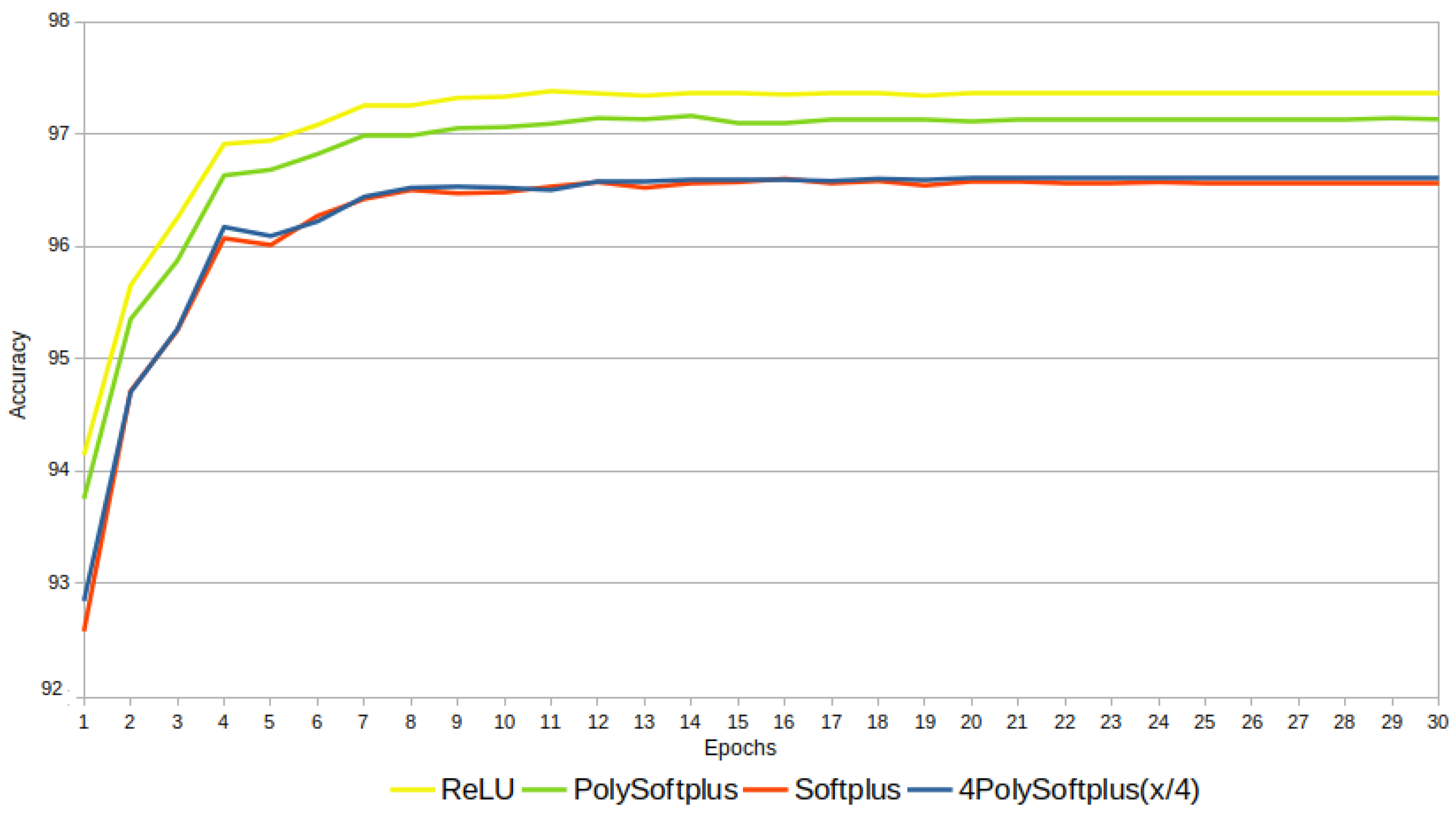
3.1. Experiment 1: PolySoftplus, Softplus, and Relu

A first experiment compares $PolySoftplus$, $PolySoftplus(\alpha ,x)$, Softplus, and ReLU. The results are shown in the plots of Figure 13. Note that:

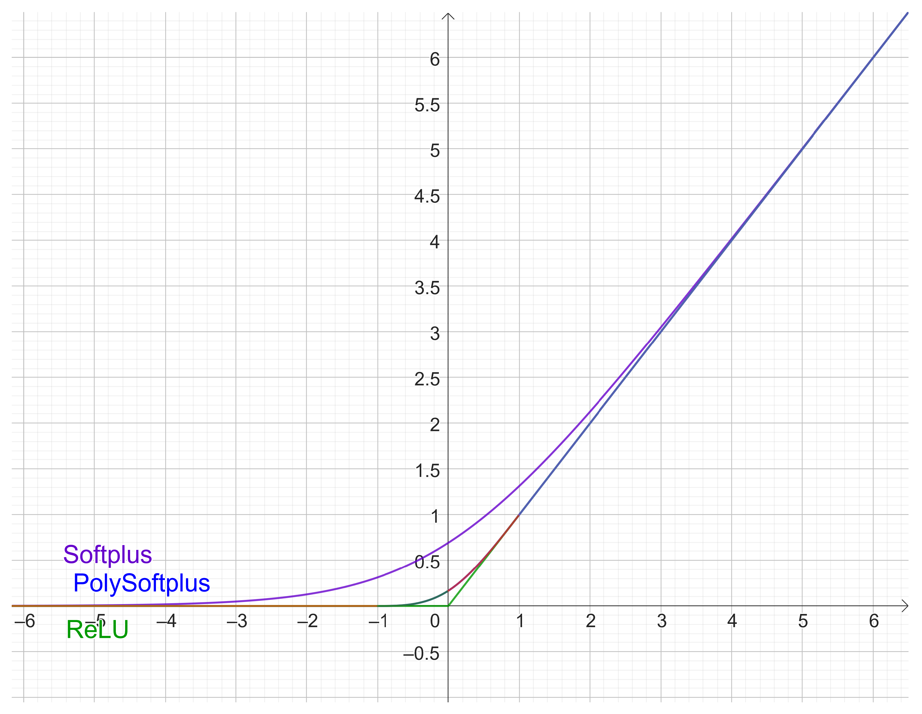
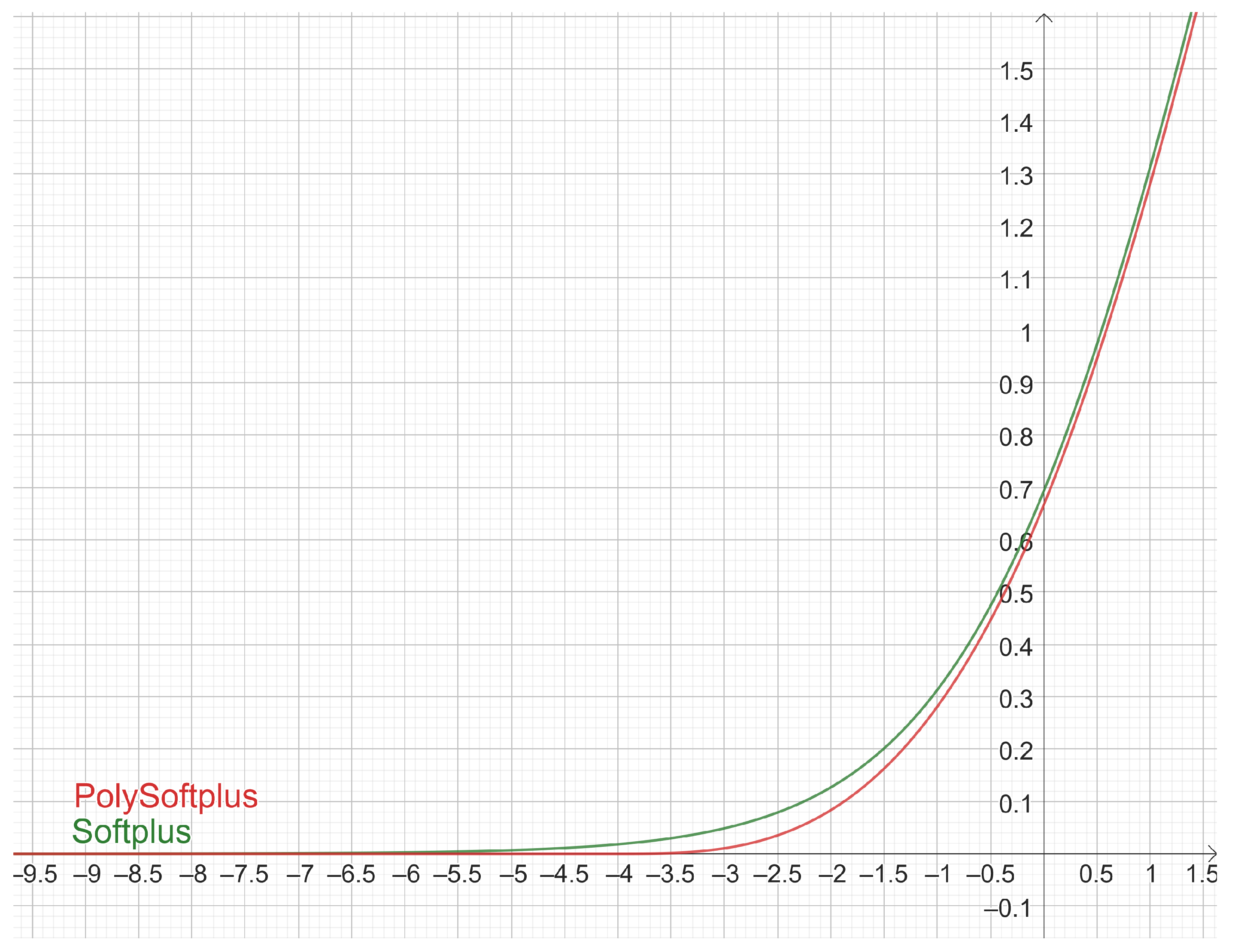
• ReLU is superior to all the other activation functions.
• PolySoftplus outperforms Softplus. It is a bit intuitive after reading Section 2.10, since PolySoftplus looks more similar to ReLU than to Softplus (see Figure 10).
• The version ${\displaystyle \frac{1}{\alpha }}PolySoftplus(\alpha ,x)$ with $\alpha ={\displaystyle \frac{1}{4}}$ is a good approximation of Softplus; therefore, it is not surprising that they produce essentially the same results.

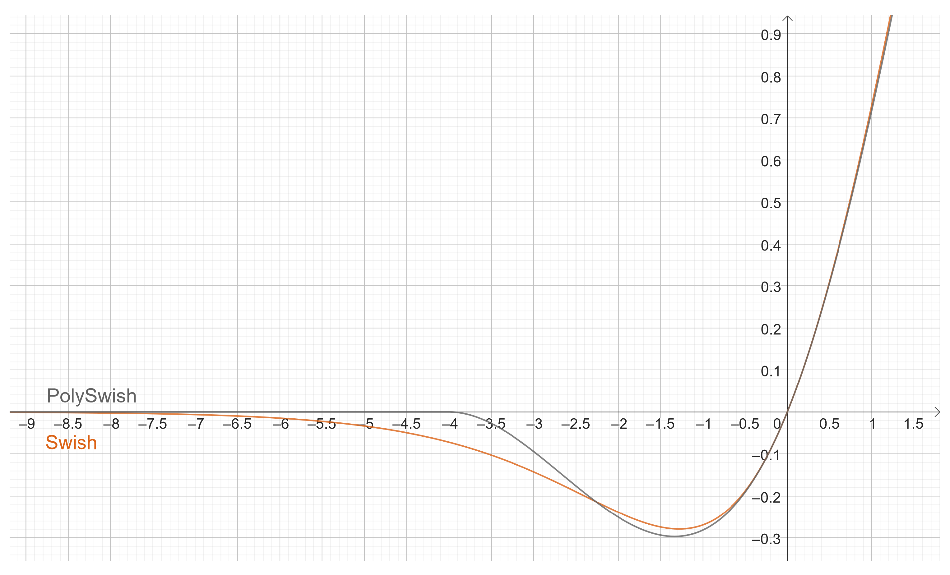
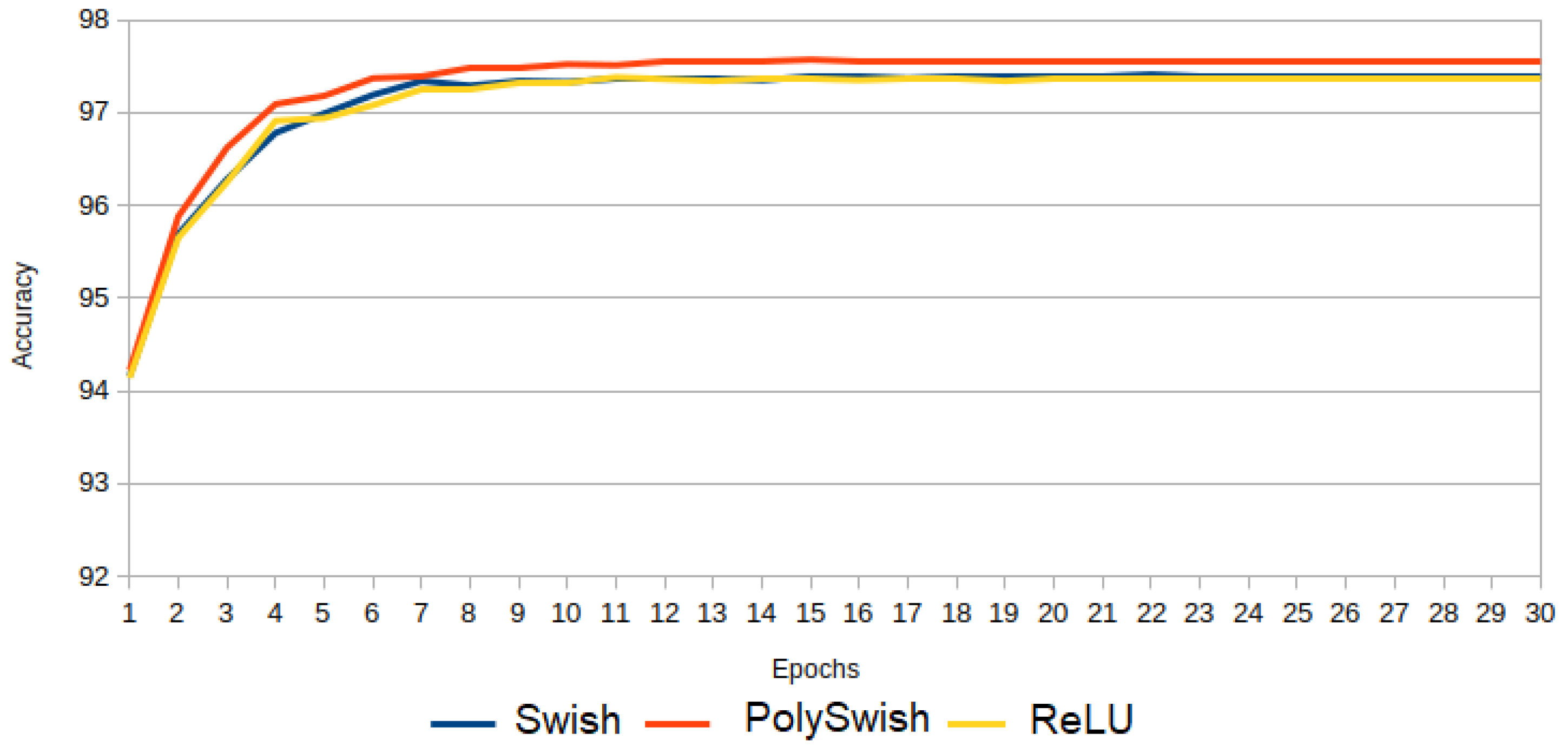
3.2. Experiment 2: PolySwish, Swish, and ReLU

In Experiment 2, PolySwish is compared with Swish and ReLU. Figure 14 shows that PolySwish is superior to Swish and ReLU. Swish is slightly better than ReLU.

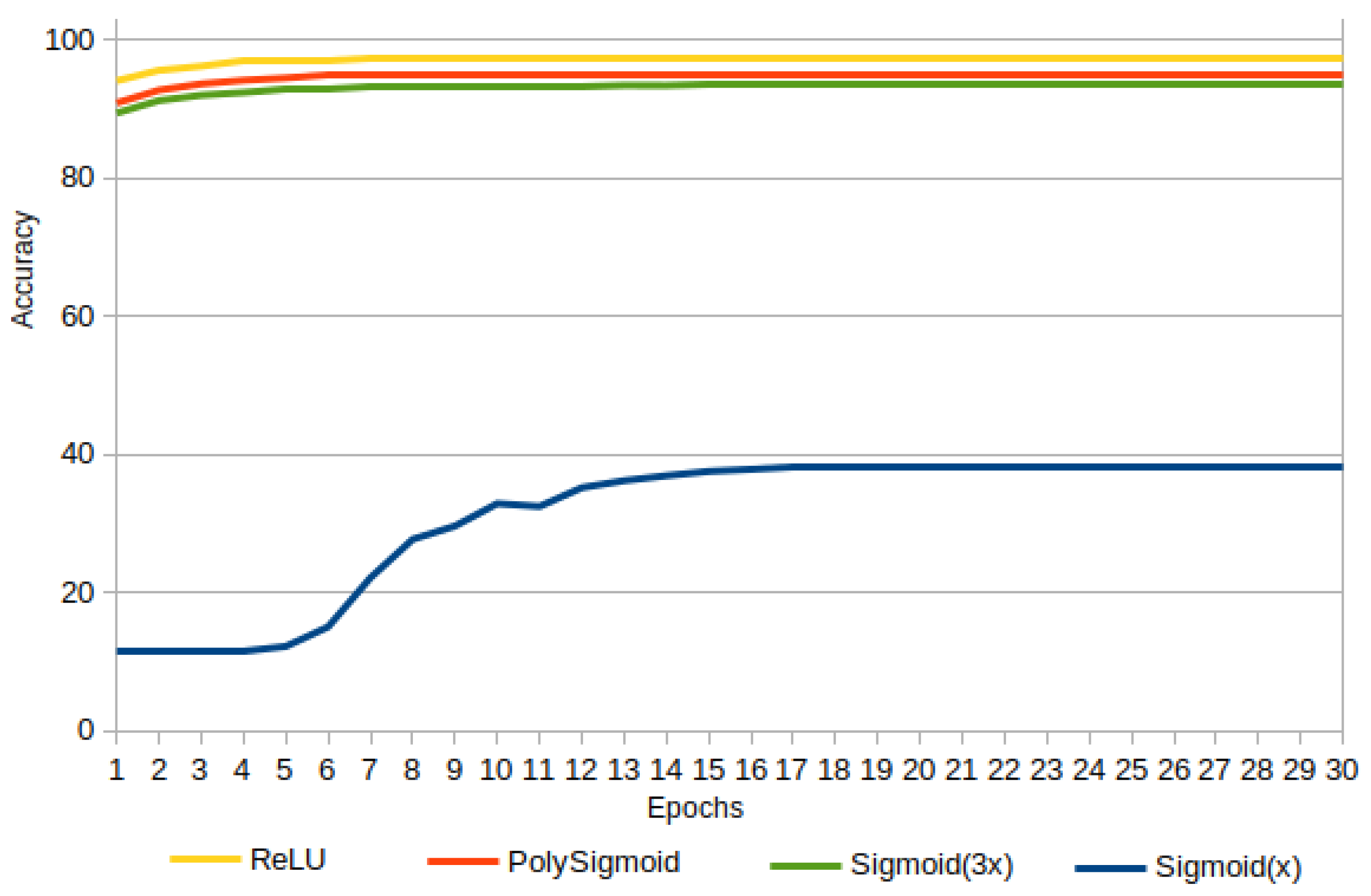
3.3. Experiment 3: PolySigmoid, Sigmoid, and ReLU

In Experiment 3, the Sigmoid performance was too low, starting with an accuracy of $11.35\%$ and reaching a maximum of $38.29\%$. For this reason, instead of the original sigmoid $\sigma \left(x\right)$, $\sigma \left(3x\right)$ was considered, and the performance was improved from $89.47\%$ up to a maximum of $93.51\%$.

Figure 15 shows the accuracies for PolySigmoid, Sigmoid $\sigma \left(x\right)$, Sigmoid $\sigma \left(3x\right)$ and ReLU. It is possible to appreciate that PolySigmoid is superior to $\sigma \left(x\right)$, and $\sigma \left(3x\right)$. However, ReLU is better than PolySigmoid and therefore better than all activation functions in this experiment.

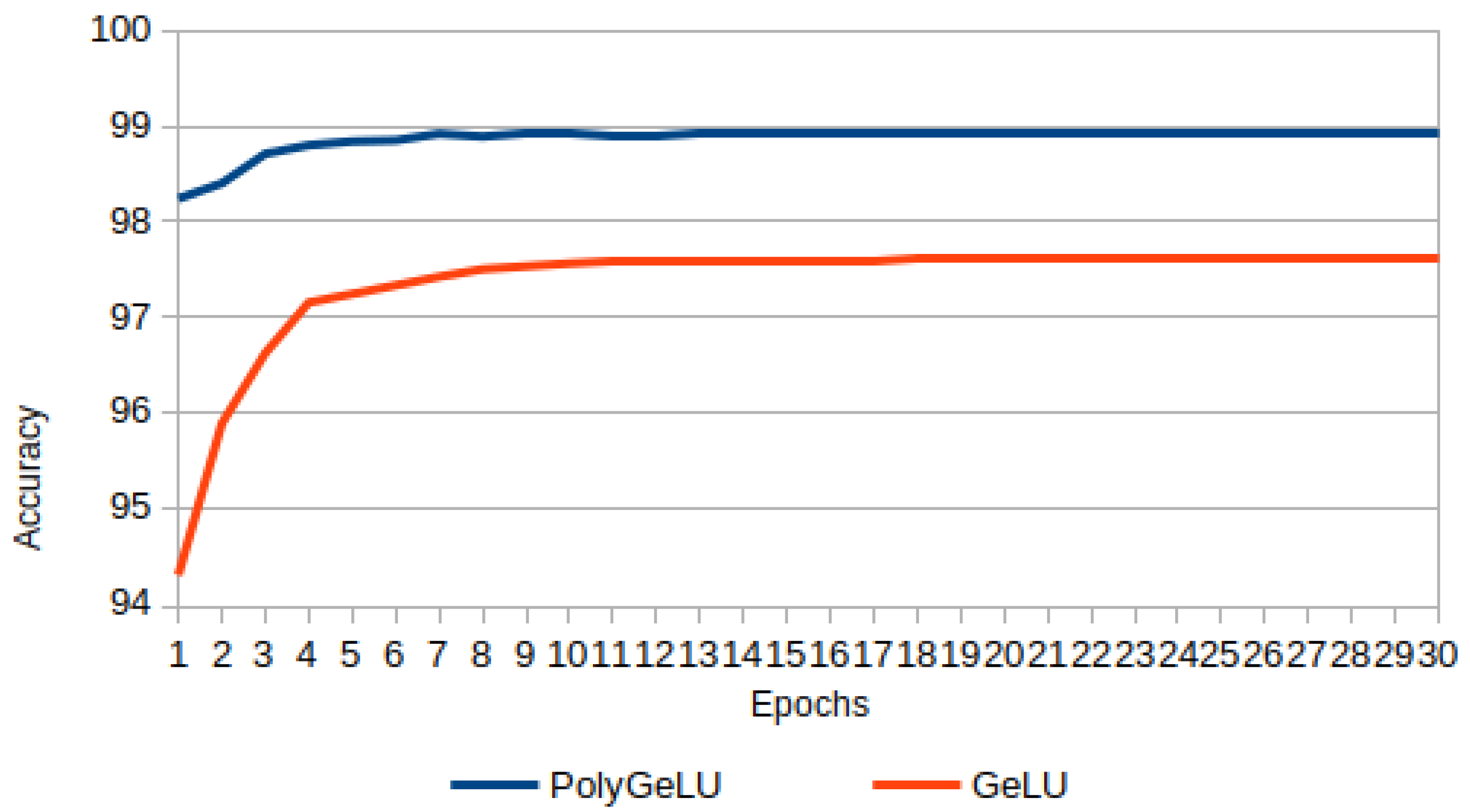
3.4. Experiment 4: PolyGeLU and GeLU

In this experiment, both activation functions, PolyGeLU (Equation (44)) and GeLU (Equation (14)), are compared. Figure 16 shows the results, where it is evident that PolyGeLU outperforms GeLU.

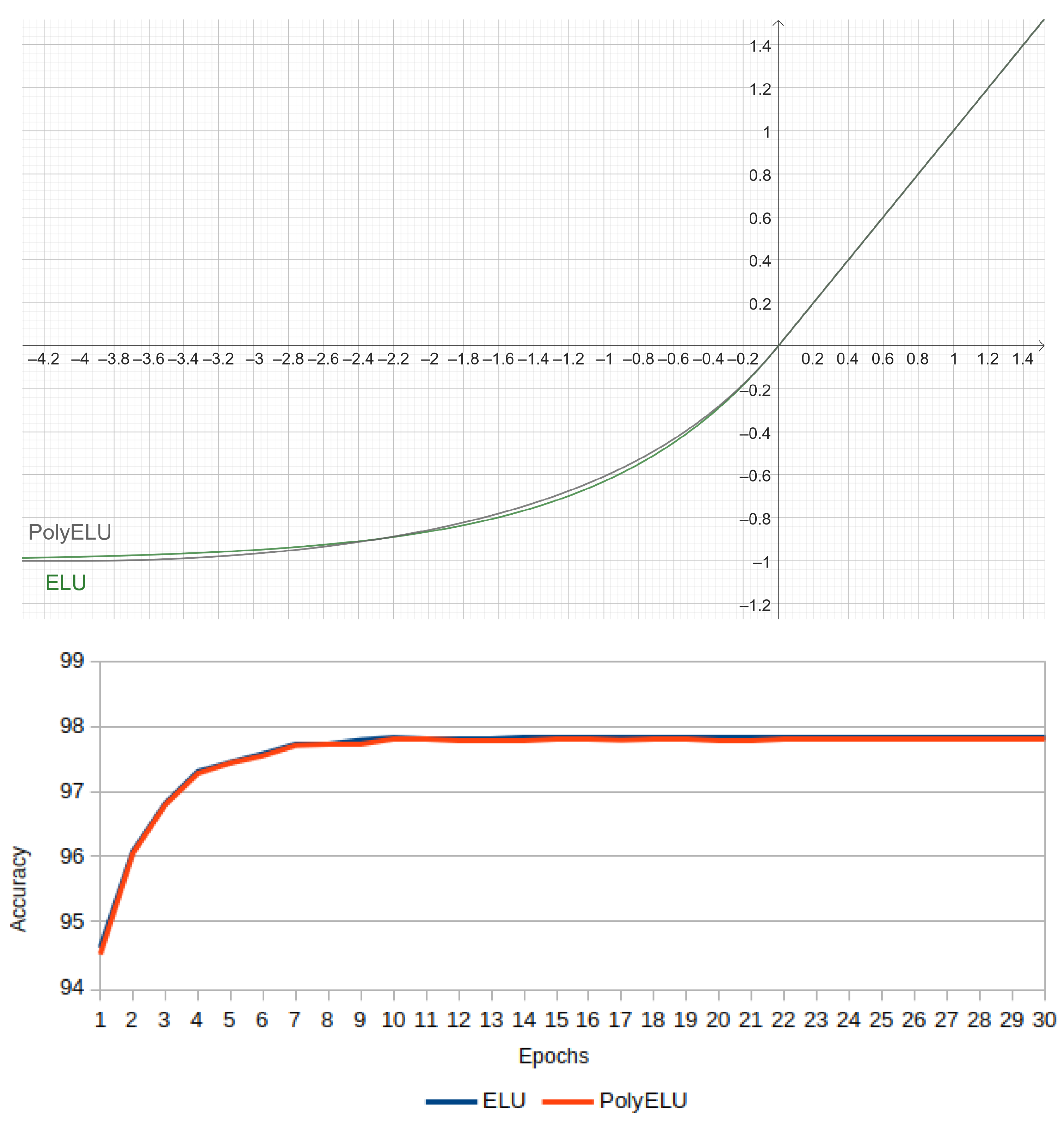
3.5. Experiment 5: ELU Approximation from PolySigmoid

In order to obtain a piecewise polynomial version of the ELU function, the following approximation is made. Given Equation (42), which approximates Sigmoid via Polysigmoid, and focusing on the interval $-4<x<0$, it follows that:

$$\sigma \left(x\right)\approx PolySigmoid({\displaystyle \frac{x}{4}})={\displaystyle \frac{{(\frac{x}{4}+1)}^2}{2}}.$$

(50)

Thus, ${\displaystyle \frac{1}{1+e^{-x}}}\approx {\displaystyle \frac{{(\frac{x}{4}+1)}^2}{2}}$, and solving for $e^x$:

$$e^x\approx {\displaystyle \frac{{(x+4)}^2}{32-{(x+4)}^2}}.$$

(51)

With this approximation, it is possible to write a polynomial version for ELU named PolyELU, so:

$$PolyELU(x,\alpha )=\{\begin{array}{cc}-\alpha \hfill & x\le -4\hfill \\ \alpha \left[{\displaystyle \frac{{(x+4)}^2}{32-{(x+4)}^2}}-1\right]\hfill & -4<x\le 0\hfill \\ x\hfill & 0<x.\hfill \end{array}$$

(52)

Figure 17 has the plots for $\alpha =1$ of PolyELU and ELU on the left side, whereas the corresponding accuracies are shown on the right side. Basically, they are overlapped and have a correlation of $0.999$. This confirms that there is a good approximation between these two activation functions.

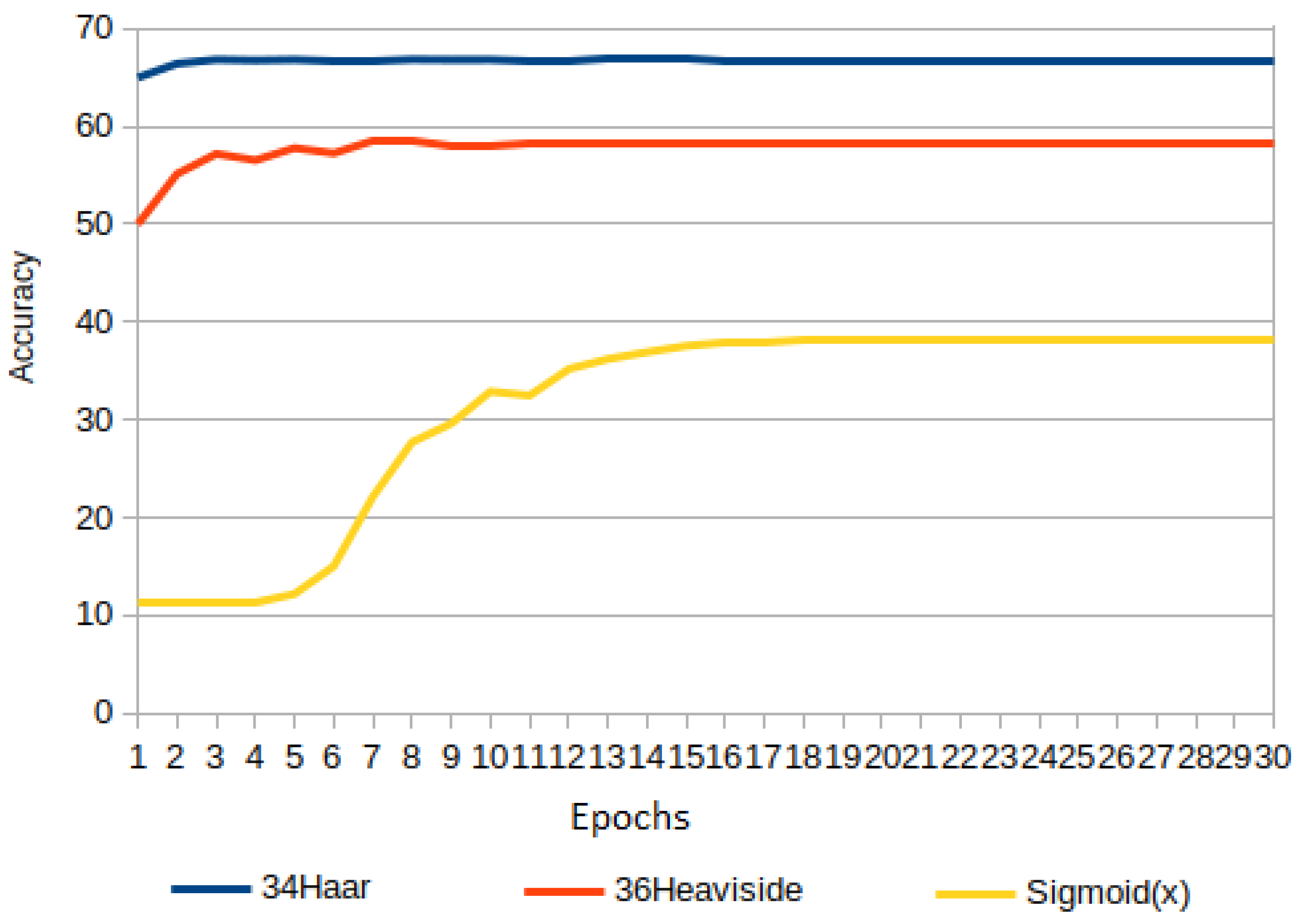
3.6. Experiment 6: Haar Wavelet, Triangular, Heaviside, and ReLU

Experiment 6 gathers some activation functions that achieve a low accuracy: Haar, Heaviside, and Sigmoid, and it is shown in Figure 18.

Haar’s accuracy is low, but higher than Heaviside and Sigmoid. Heaviside varies from $49.99\%$ up to $58.22\%$, whereas Sigmoid is below $40\%$. It is striking how a Sigmoid function that approaches Heaviside as $\alpha$ tends to infinity can increase its accuracy. It has been experimentally calculated that as $\alpha$ increases up to $19.459$, the accuracy improves. In fact, the accuracy of Sigmoid with high $\alpha$-value outperformed that of Heaviside.

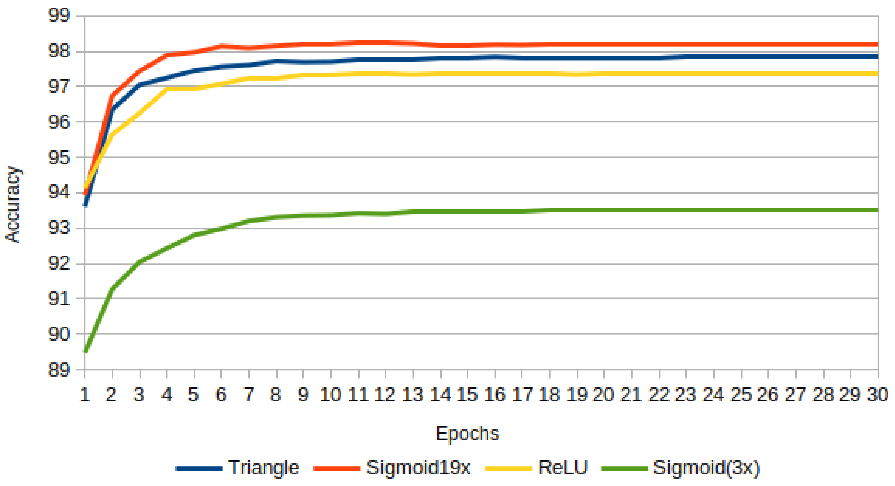
Obtaining the maximum accuracy for Sigmoid($19.459x$), it was compared with Triangular and ReLU. The results are in Figure 19, where Sigmoid($19.459x$) outperforms Triangular followed by ReLU. Sigmoid($3x$) was also plotted just as a reference.

This experiment leads us to consider the importance of the non-zero gradient problem, challenging for Haar and Heaviside, which is extensive to Sigmoid for high scaling factors.

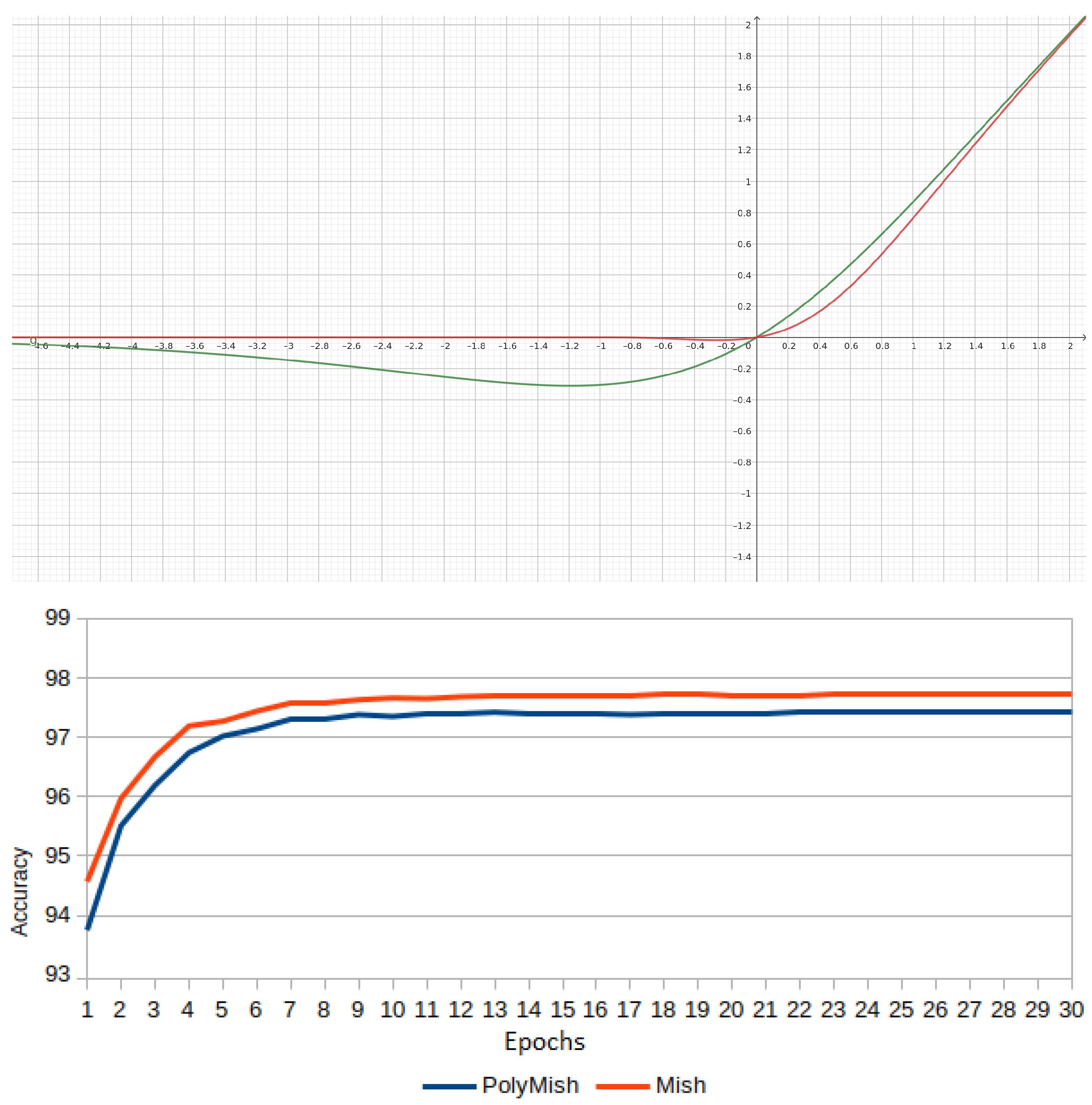
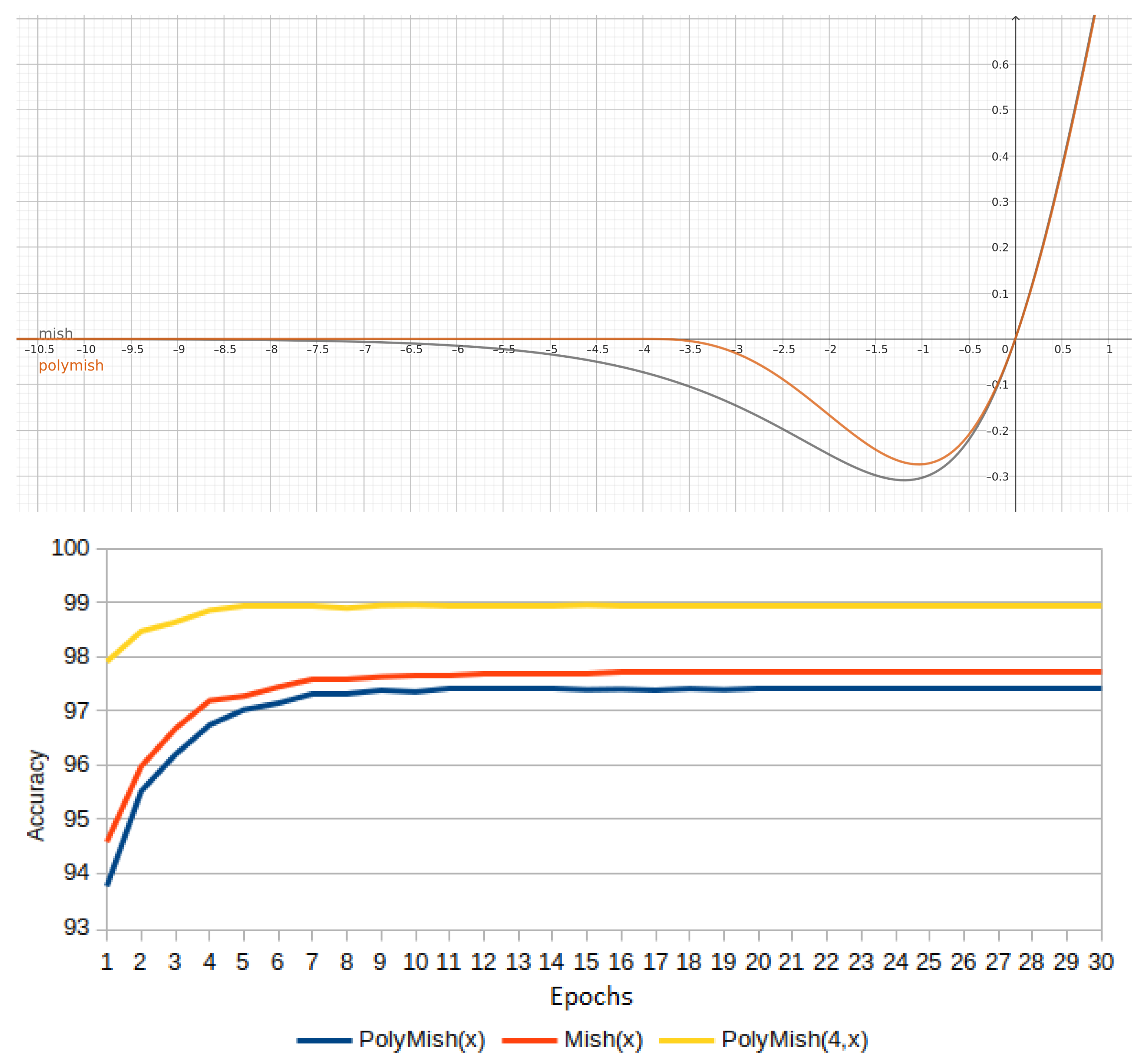
3.7. Experiment 7: Mish and PolyMish

Given the definition of PolySoftplus(x) in Equation (45), and some advantages over Softplus described in Section 3.1, is natural to propose a first Mish approximation named PolyMish, as follows:

$$PolyMish\left(x\right)=x·tanh\left(PolySoftplus\right(x\left)\right).$$

(53)

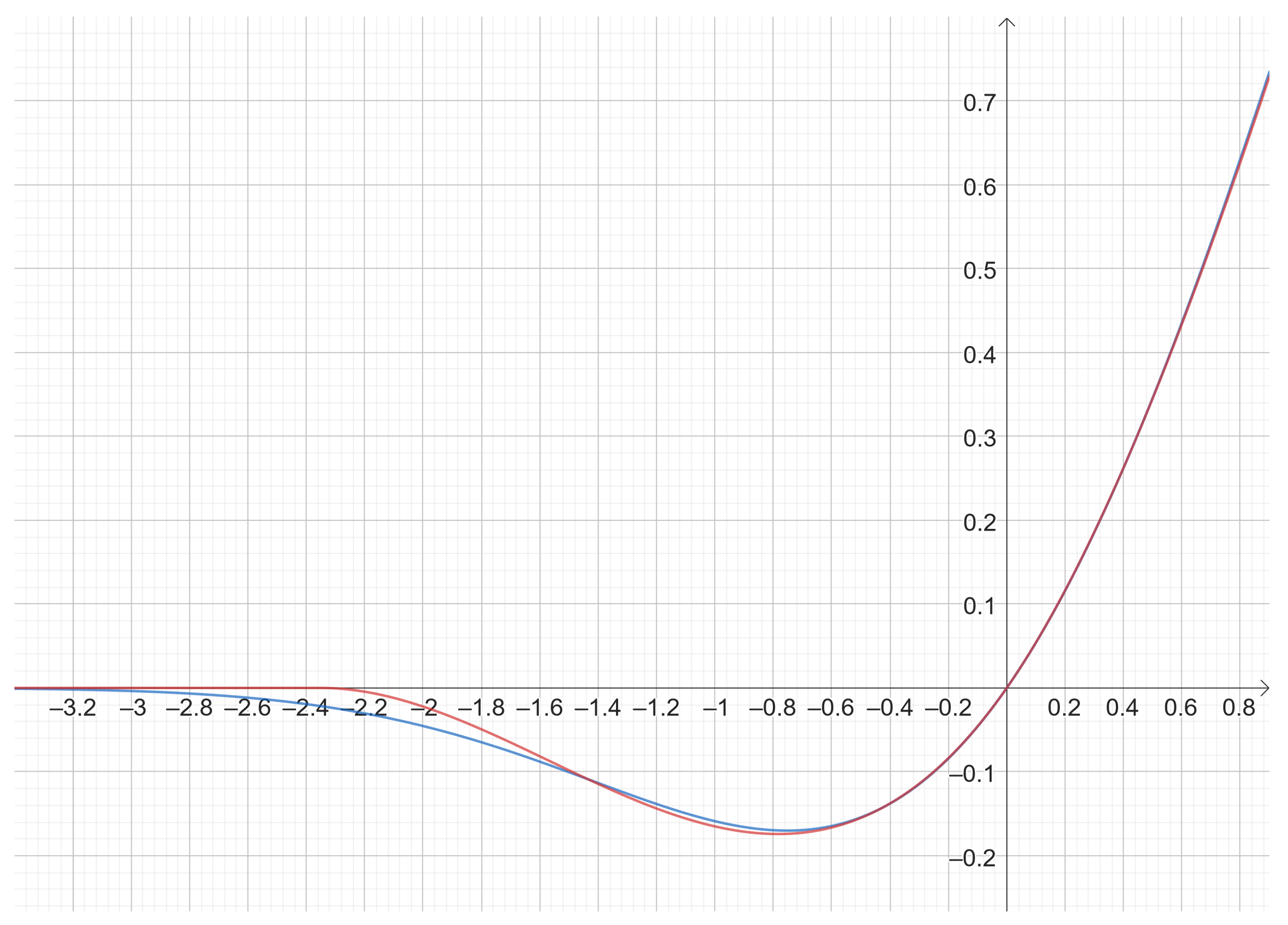
Figure 20 shows the plots of Mish vs. PolyMish. Mish(x) follows a smooth curve for $x<0$ and asymptotical behavior to zero for $x<-1.2$, whereas PolyMish vanishes faster than Mish and is exactly zero for $x<-1$ (see Section 3.7). In other words, this first version is not a good approximation. Moreover, the bottom side of Figure 20 illustrates how Mish outperforms PolyMish.

The approximation to Mish can be improved by considering an $\alpha$ factor, as in Section 3.1, so that:

$$PolyMish(\alpha ,x)=x·tanh(\alpha ·PolySoftplus\left({\displaystyle \frac{x}{\alpha }}\right)).$$

(54)

The top side of Figure 21 shows the approximation of Mish using $PolyMish(\alpha =4,x)$. The accuracy results are shown on the bottom side of Figure 21, where it is noticeable that this second version of $PolyMish(\alpha =4,x)$ outperforms Mish.

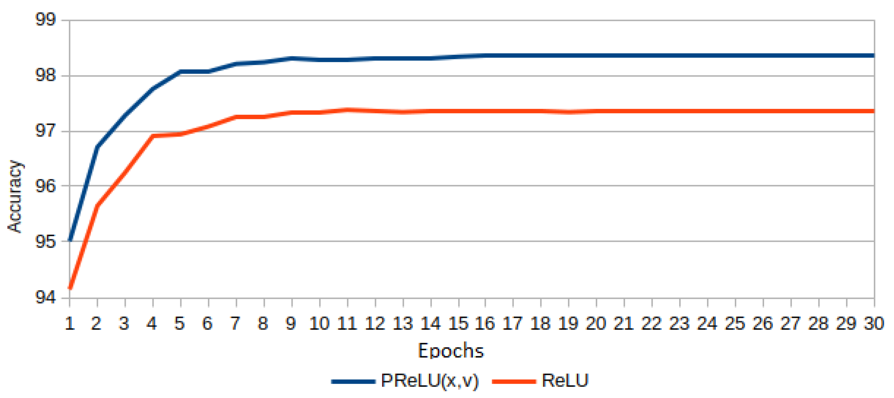
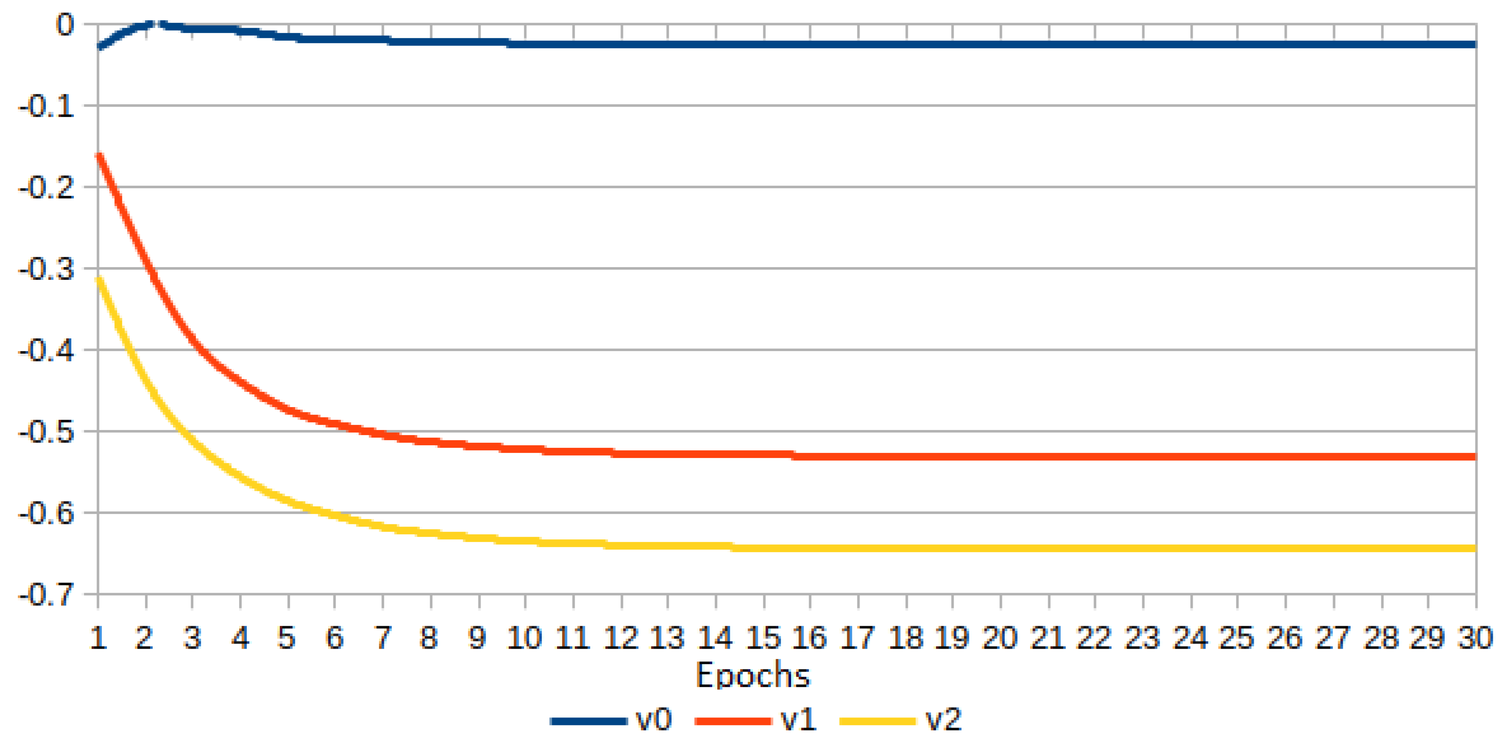
3.8. Experiment 8: Adaptive Fractional Derivative Order for $PReLU(x,\nu )$ vs. $ReLU\left(x\right)$

In this experiment, given $PReLU(x,\nu )$, the parameter $\nu$ is adapted during the learning (see Equation (33)). The initial value for $\nu$ is zero. The network architecture involves three $PReLU(x,\nu )$ functions, and each $\nu$-parameter is adjusted with SGD as a hyperparameter in Pytorch. The results are shown in Figure 22. From the top side, it is evident that the PReLU version outperforms the network built only with ReLUs. The adaptive $\nu$-values for the three PReLUs are shown at the bottom of Figure 22, where the fractional derivatives have negative values, i.e., the power of x is greater than $1.0$.

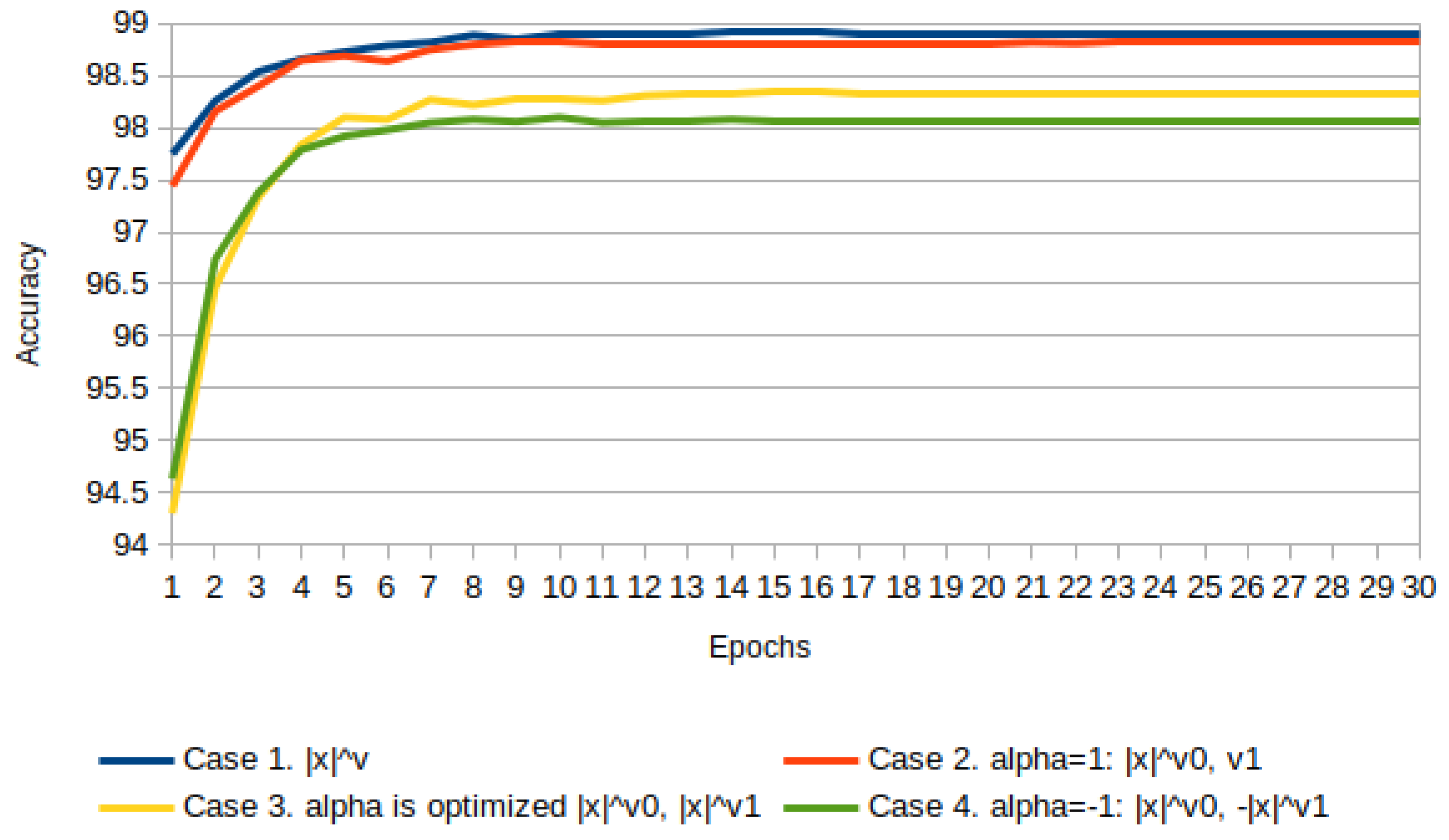
3.9. Experiment 9: Fractional Derivative of $\left|x\right|$ as Activation Function

The importance of having a non-zero gradient for $x\le 0$ is a motivation to use a fractional derivative of $\left|x\right|$ based on Equations (33) and (34), as follows:

$${\left|x\right|}^{\nu }=D_x^{\nu }\left|x\right|=\{\begin{array}{cc}{\displaystyle \frac{{(-x)}^{1-v}}{\mathsf{\Gamma }(2-v)}}\hfill & x\le 0\\ {\displaystyle \frac{x^{1-v}}{\mathsf{\Gamma }(2-v)}}\hfill & 0<x.\end{array}$$

(55)

Beyond this, different fractional-order derivatives can be used, ${\nu }_0$ for $x\le 0$ and ${\nu }_1$ for $x>0$. Thus, for $\alpha \in \mathbb{R}$:

$${\left|x\right|}^{{\nu }_0,{\nu }_1}=D_x^{{\nu }_0,{\nu }_1}\left|x\right|=\{\begin{array}{cc}\alpha {\displaystyle \frac{{(-x)}^{1-v_0}}{\mathsf{\Gamma }(2-v_0)}}\hfill & x\le 0\\ {\displaystyle \frac{x^{1-v_1}}{\mathsf{\Gamma }(2-v_1)}}\hfill & 0<x.\end{array}$$

(56)

If ${\nu }_0>1$, then Equation (56) produces a zero division if $x=0$, but to avoid this situation, it is possible to add an $ϵ>0$ [18]. In this experiment, $ϵ=1e-10$.

Results of four cases are reported in Figure 23, sorted from best to worst:

• Case 1. ${\left|x\right|}^{\nu }$, Equation (55).
• Case 2. ${\left|x\right|}^{{\nu }_0,{\nu }_1}$, Equation (56) $\alpha =1$.
• Case 3. ${\left|x\right|}^{{\nu }_0,{\nu }_1}$, Equation (56), where $\alpha$ is optimized with SGD as hyperparameter.
• Case 4. ${\left|x\right|}^{{\nu }_0,{\nu }_1}$, Equation (56) $\alpha =-1$.

All $\nu$-parameters as well as $\alpha$ are initialized to zero. For Case 3, $\alpha$ is optimized in three activation functions AF1, AF2, and AF3.

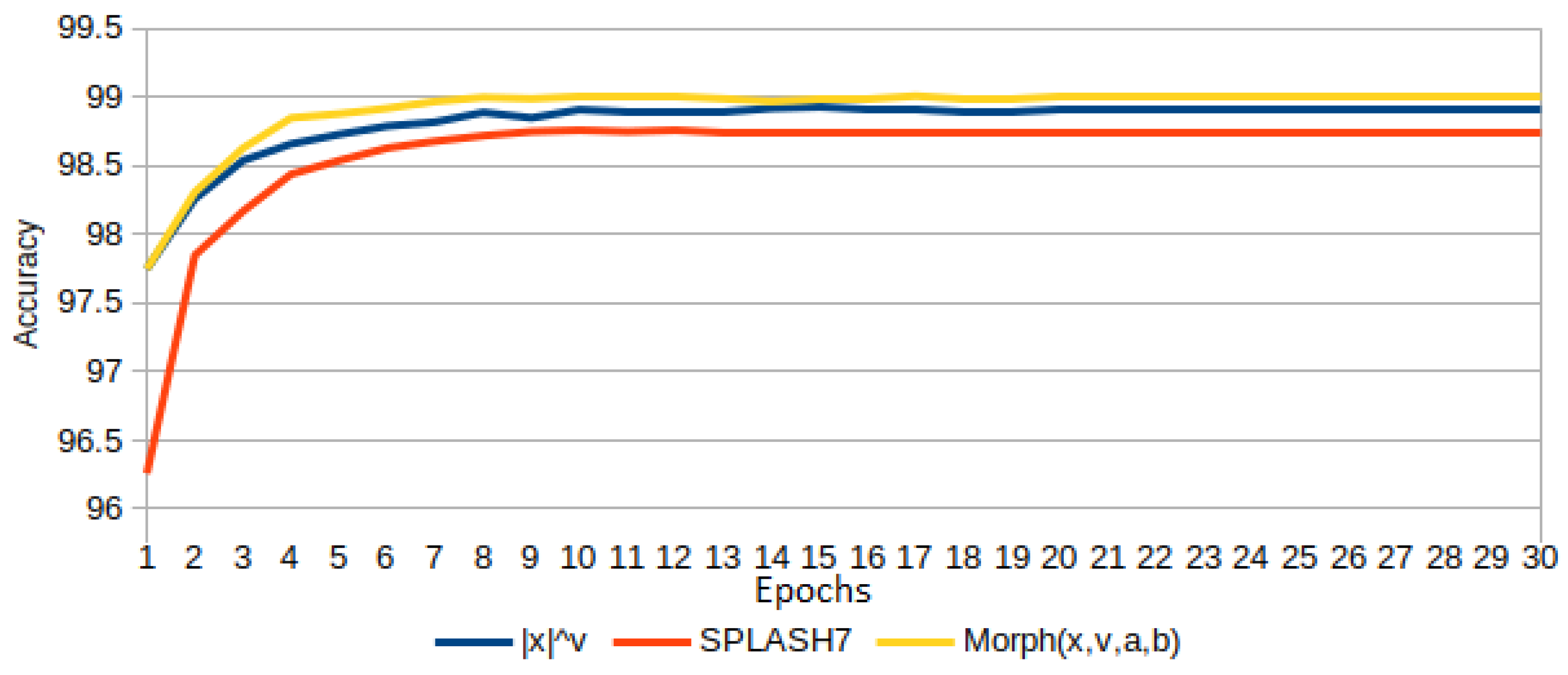
3.10. Experiment 10: Trainable Activation Functions with Fractional Order: $Morph$ and ${\left|x\right|}^{\nu }$ vs. SPLASH

In this experiment, the adaptive $\nu$-order of fractional functions is optimized with SGD in PyTorch. Three activation functions are compared: SPLASH, ${\left|x\right|}^{\nu }$, and $Morph$.

From Equation (30), only seven terms are considered for SPLASH, then it is written as:

$$SPLAS{H}_7\left(x\right)=a_{0}max(0,x)+\sum _{s=1}^3{a}_{+}^{s}max(0,x-b^s)+\sum _{s=1}^3{a}_{-}^{s}max(0,-x-b^s)$$

(57)

where $b^s=\{1,2,2.5\}$, $a_0$ is initialized to one, and the rest to zero (see [20]). These initial conditions mean initializing with ReLU shape. SPLASH does not involve fractional derivatives, but it is used in this experiment as a reference for comparison purposes.

The neural network architecture has three activation functions, and for SPLASH, each unit needs seven a-parameters. So, the total number of hyperparameters is 21 (it certainly consumes enough GPU memory).

For the fractional derivative ${\left|x\right|}^{\nu }$ of Equation (55), the total number of hyperparameters is 3, and the initialization was $\nu =0$, which means initializing with a piecewise linear shape.

In the case of Morph, dilation a and translation b are used, so $Morph(x,\nu ,a,b)=Morph({\displaystyle \frac{x-b}{a}},\nu )$ and the initialization was $\nu =-2.0$, $a=1$, and $b=0$. It corresponds to PolySoftplus of Equation (45) illustrated in Figure 10 (a shape similar to ReLU or Softplus, in Section 2.10). In this case, $Morph(x,\nu ,a,b)$ needs to adapt $3\times 3=9$ hyperparameters.

The accuracy results are show in Figure 24. SPLASH adjust all of the $7\times 3=21$ parameters, but its performance is lower than the corresponding of ${\left|x\right|}^{\nu }$, which, by the way, only uses three parameters.

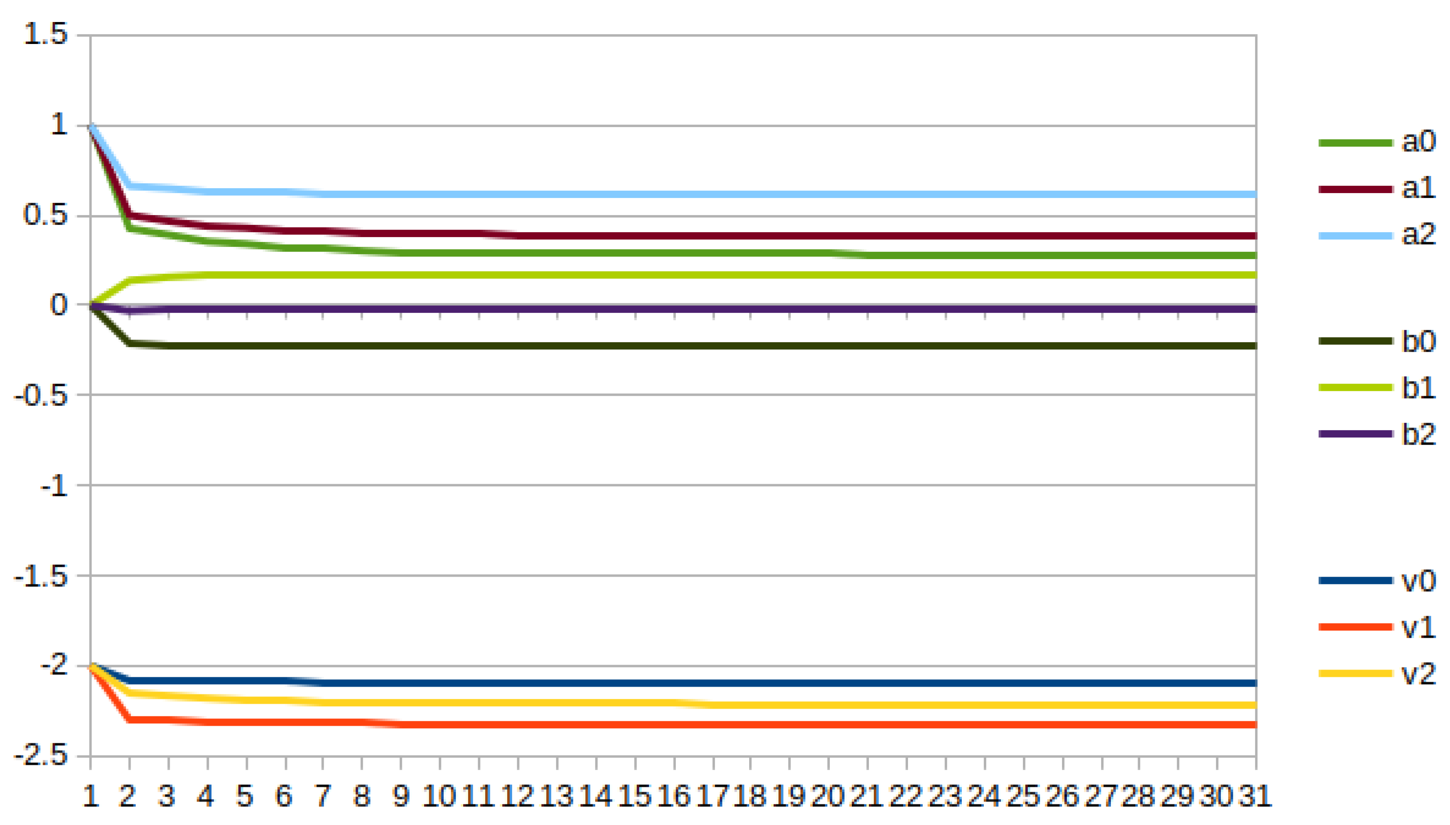
Special attention is given to $Morph(x,\nu ,a,b)$, which achieves the best accuracy compared to ${\left|x\right|}^{\nu }$ and $SPLAS{H}_7$.

Figure 25 shows the change of the fractional orders of three $Morph\left(\right)$ activation functions used in the network architecture: ${\nu }_0$, ${\nu }_1$, and ${\nu }_2$ initialized to zero. Also, the parameters a and b of these three $Morph\left(\right)$ functions are optimized, and they are plotted in the same figure.

Figure 26 shows the shape of $Morph(x,\nu ,a,b)$ when the parameters $\nu =-2,a=1,$ $b=0$ are updated to $\nu =-2.0932,a=0.3014,b=-0.2269$, and then to $\nu =-2.0959,$ $a=0.2829,$ $b=-0.2295$ at epochs 0, 2, and 30, respectively. These parameters are optimized with the gradient descent algorithm SGD in PyTorch. Only the values of one of the three Morph functions are presented for reasons of space, and since they are similar to those of the other two units.

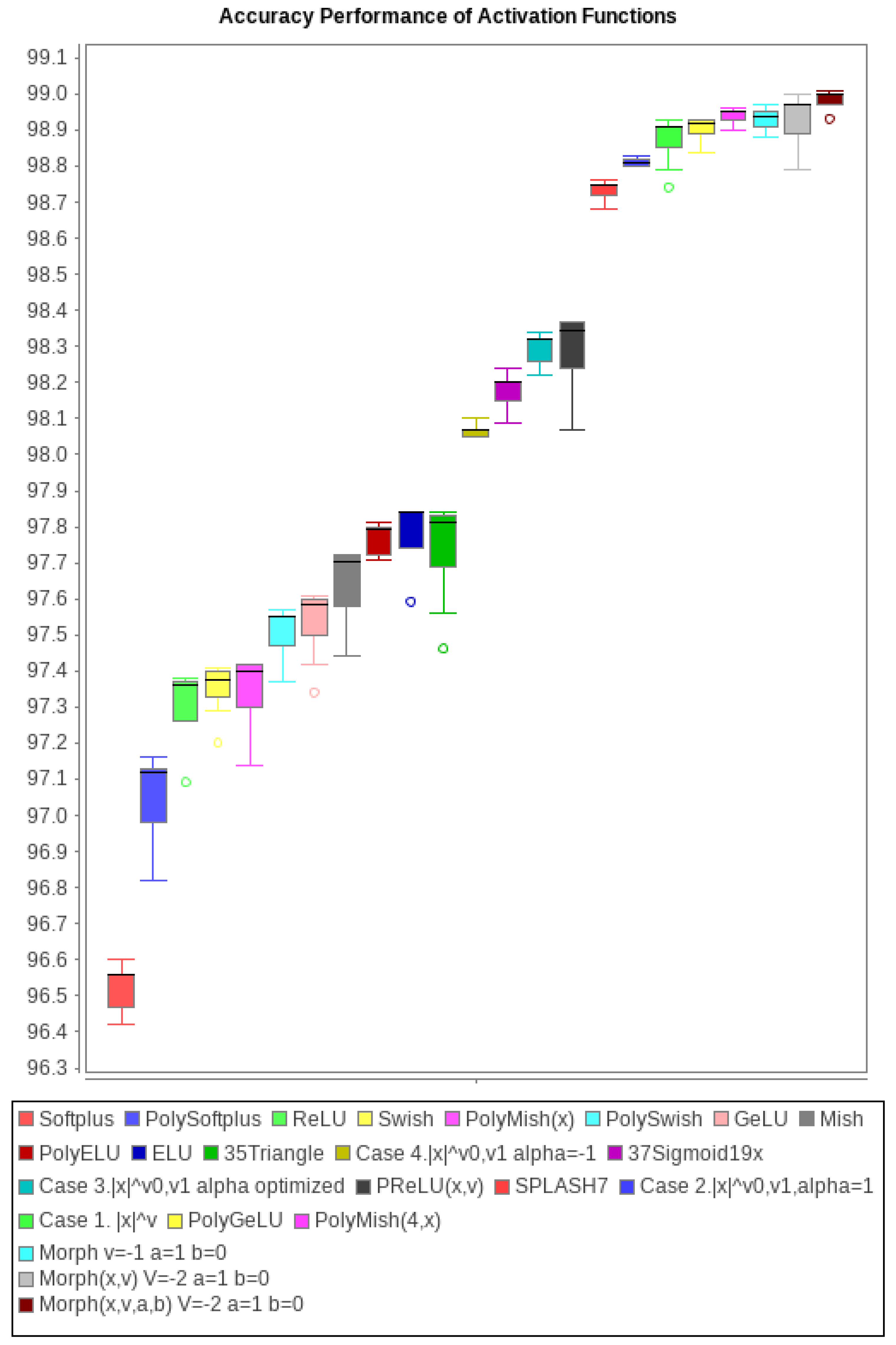
3.11. Experiment 11: Comparison of Morph() with Other 20 Activation Functions

Experiment 11 compares several activation functions: piecewise polynomial obtained as special cases of $Morph\left(\right)$ and other existing and well-known activation functions. Based on the accuracy results, they are shown in Figure 27 sorted from left to right, worst to best, and enumerated in

Table 1. Comparison of activation functions, worst to best on MNIST dataset, sorted by test accuracy.

1, Softplus (lowest accuracy) 2. PolySoftplus 3. ReLU 4. Swish 5. PolyMish 6. PolySwish 7. GeLU 8. Mish 9. PolyELU 10. ELU 11. Triangular 12. Case 4.${\left|x\right|}^{v_0,v_1},\alpha =-1$

13. Sigmoid($19x$) 14. Case 3.${\left|x\right|}^{v_0,v_1},\alpha$ optimized 15. $PReLU(x,v)$ 16. $SPLAS{H}_7$ 17. Case 2.${\left|x\right|}^{{\nu }_0,{\nu }_1},\alpha =1$ 18. Case 1. ${\left|x\right|}^{\nu }$ 19. PolyGeLU 20. PolyMish$(4,x)$ 21. $Morph(x,\nu )$, $\nu =-1,a=1,b=0$ 22. $Morph(x,\nu )$, $\nu =-2,a=1,b=0$ 23. $Morph(x,\nu ,a,b)$, $\nu =-2,a=1,b=0$ (highest accuracy)

. Highlighted in bold are cases where a polynomial version is better than its counterpart, for example, PolySoftplus is better than Softplus. Note that the highest accuracies are achieved by $Morph$ with optimized parameters:

Case 21. $Morph(x,\nu )$, initializes $\nu =-1,a=1,b=0$ and $\nu$ is optimized during the training.

Case 22. $Morph(x,\nu )$, initializes $\nu =-2,a=1,b=0$ and $\nu$ is optimized during the training.

Case 23. $Morph(x,\nu ,a,b)$, initializes $\nu =-2,a=1,b=0$ and $\nu ,a,b$ are optimized during the training.

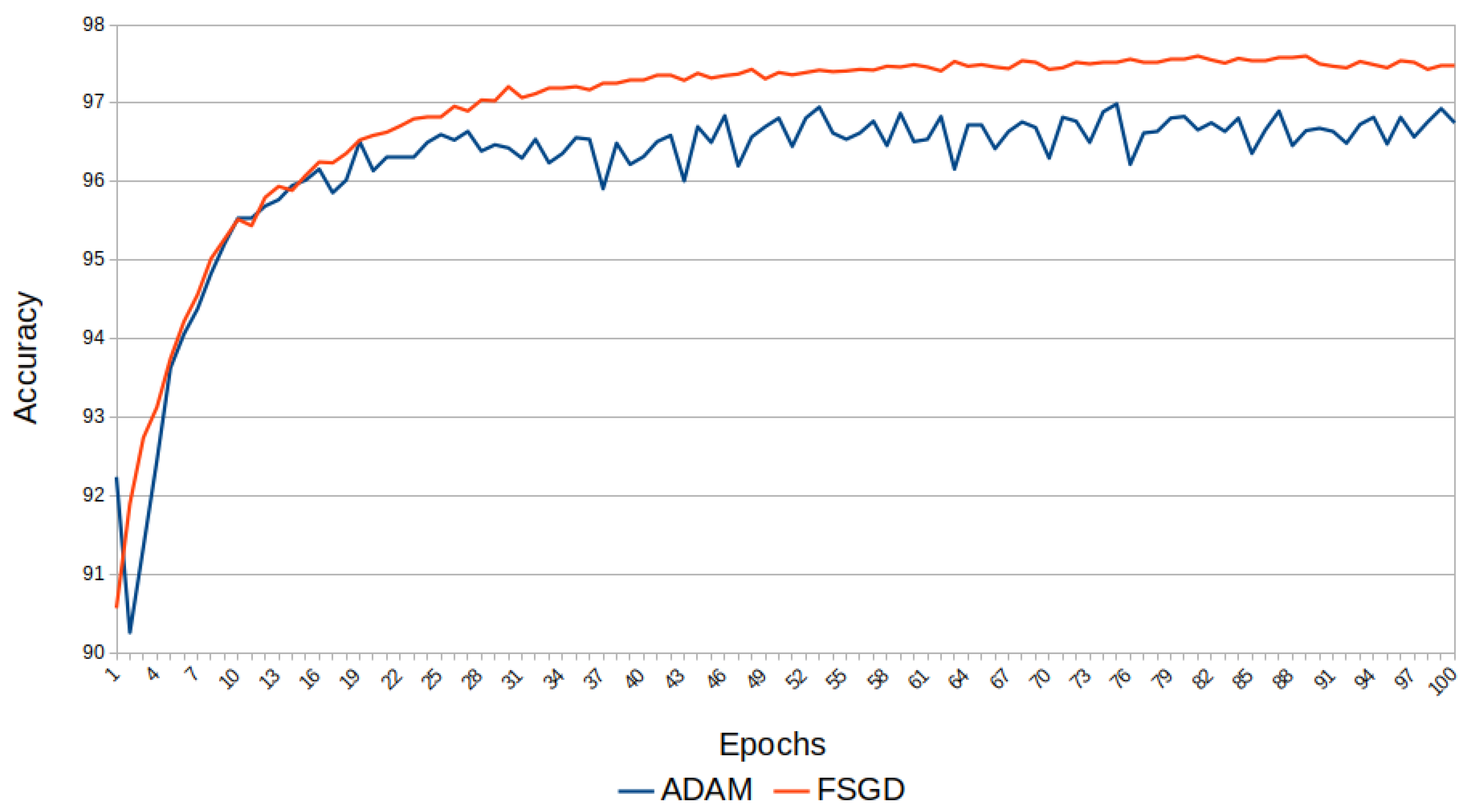
3.12. Experiment 12: Adapting Morph with SGD and Adam

Finally, in the last experiment, a minimal neural network is used to illustrate how the fractional derivative $\nu$ for $Morph\left(\right)$ is updated using Adam and a fractional SGD (FSGD) [19] with the fractional gradient set to $1.7$, which was determined experimentally for MNIST [18,19]. Note that the fractional gradient uses the fractional derivative of the activation function to update the learning parameters, but the approach is different (and complementary) to adjust the shape of the fractional derivative for $Morph\left(\right)$ as activation function.

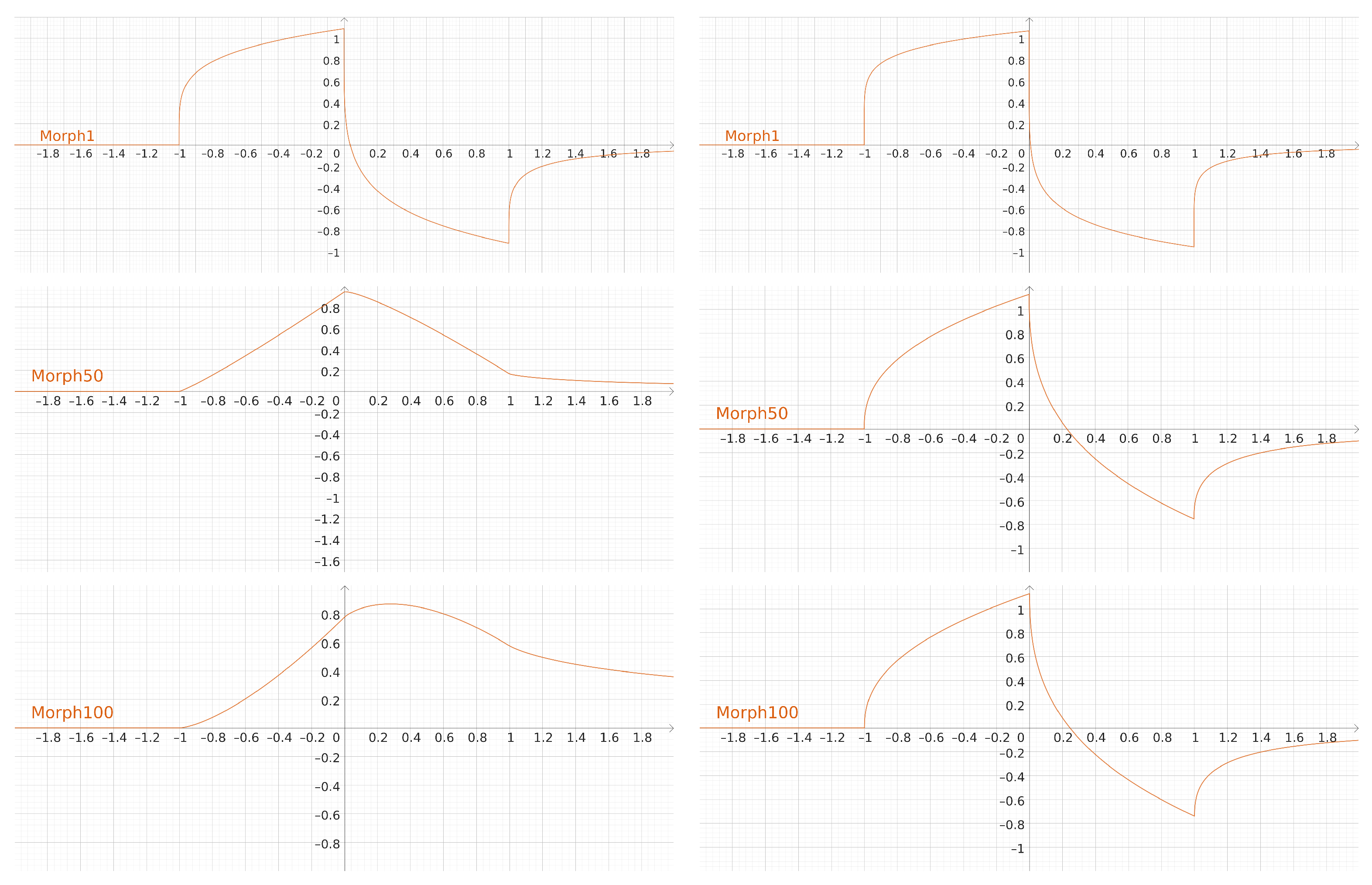
The number of epochs was 100, and the accuracy results are shown in Figure 28. The parameter initialization is $\nu =0.75$. In Figure 29, the shapes for epochs $1,50$, and 100 are plotted for both Adam and FSGD. It is a demonstration that a fractional optimizer like SGD can be sufficiently competitive with other more sophisticated optimizers like Adam. In fact, FSGD outperforms Adam in this experiment.

The source code of all the experiments is available at http://ia.azc.uam.mx accessed on 11 July 2024.

4. Discussion

One of the branches of artificial intelligence research is the architecture of neural networks, focused on the number of layers, types of modules, and their connections. However, another branch that has gained traction is proposing new activation functions that provide the non-linearity required by neural networks to efficiently map inputs to outputs of complex data.

Fractional calculus emerges as a mathematical tool to generalize to non-integer derivative orders, useful for building activation functions and, in this paper, a novel adaptive activation function $Morph$ was proposed based on fractional derivatives.

The search for the best activation function has led to the proposal of adaptive functions that learn from data. The adjustment of hyperparameters allows us to control stability, overfitting, and to enhance the performance of neural networks, among other challenges in machine learning.

Although we are certainly not working on function approximation with $Morph$, but rather using it as an activation function, it is important to emphasize the approximation property of $Morph$, and consequently to remark on how it provides the nonlinearity needed in a neural network to efficiently map inputs to outputs with good generalization capacity.

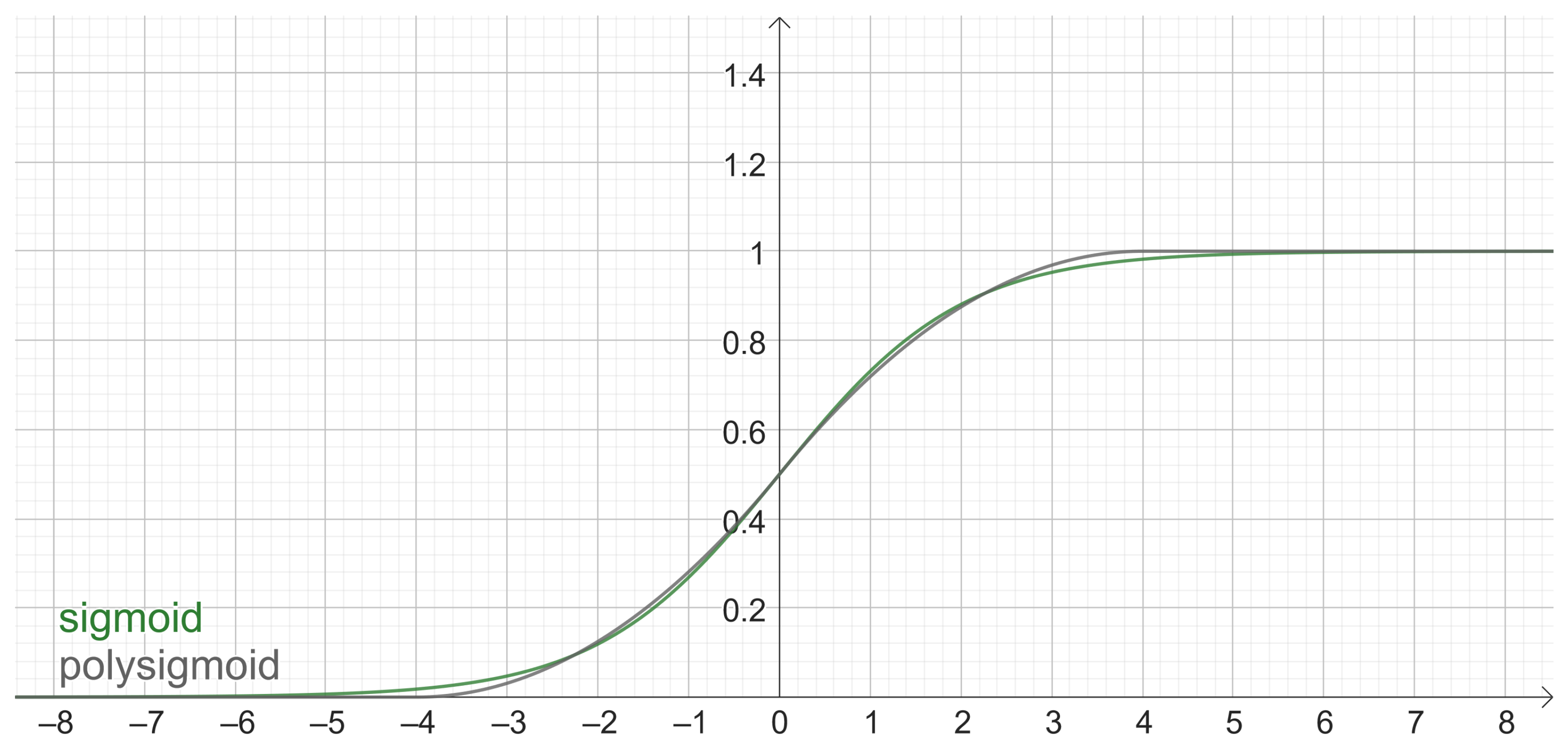
The proposed $Morph$ function approximates the Sigmoid function sufficiently to satisfy the conditions of the Universal Approximation Theorem [37]. Thus, there is a theoretical justification for $Morph$ to approximate functions in compact subspaces.

Also, $Morph$ is able to mimic shapes such as the Haar wavelet, which in turn are basis functions of vector spaces, and it gives an idea of the approximation capacity of this proposed function [43]. In fact, the inspiring idea for $Morph$ relies on the Haar decomposition as a linear combination of translated Heaviside functions.

Indeed, two fundamental operations on functions are translation and dilation [43]. In this way, for $a\ne 0$ and $b\in \mathbb{R}$, the translated and dilated version of $Morph(x,\nu )$ is:

$$Morph(x,\nu ,a,b)=Morph({\displaystyle \frac{x-b}{a}},\nu ).$$

(58)

A successful application of this was the approximation of Sigmoid via PolySigmoid, Swish via PolySwish in Section 2.7, and GeLU via PolyGeLU in Section 2.9.

Given that several activation functions include x as a factor, an adaptation to $Morph$ is $Morphx$, which can be defined as:

$$Morphx(x,\nu ,a,b,c,d,p)=c·x^p·Morph({\displaystyle \frac{x-b}{a}},\nu )+d$$

(59)

where $a\ne 0$, $b,c,d\in \mathbb{R}$, $\nu \in (-\infty ,1)$ and $p=\{0,1\}$.

Considering this, other activation functions such as tanh can be written using $Morphx$. For example, starting with the parameters for Sigmoid $\nu =-1,a=4,b=0,c=1,d=0$, and $p=0$, it is possible to write $2\sigma \left(2x\right)\approx Morphx(x,-1,2,0,2,0,0)$, and consequently:

$$tanh\left(x\right)=2\sigma \left(2x\right)-1=Morphx(x,-1,2,0,2,-1,0).$$

(60)

Table 2. Special cases of $Morphx(x,\nu ,a,b,c,d,p)$.

Shape	Approximation	$\nu$	a	b	c	d	p
Haar	Haar	1	1	0	1	0	0
Triangular	Triangular	0	1	0	1	0	0
Sigmoid	PolySigmoid	−1	4	0	1	0	0
Swish	PolySwish	−1	4	0	1	0	1
GeLU	PolyGeLU	−1	${\displaystyle \frac{4}{1.702}}$	0	1	0	1
ReLU	PolySoftplus	−2	1	0	1	0	0
Softplus	PolySoftplus	−2	4	0	4	0	0
ELU	PolyELU *	−1	4	0	1	0	0
Polynomial	Polynomial	$<-2$	$\ne 0$	-	$\ne 0$	0	0
tanh	$2\sigma \left(2x\right)-1$	−1	2	0	2	−1	0
ReLU	PolySigmoid	−1	$a\to 0^{+}$	0	1	0	1

* Approximating $e^x$ in $-4<x\le 0$.

summarizes important cases of $Morphx(x,\nu ,a,b,c,p)$ that allow us to obtain shapes that sufficiently approximate existing activation functions.

$Morph$ not only allows us to obtain good approximations, but also provides formulas of piecewise polynomial versions of activation functions which could improve computational efficiency.

Future work includes proposing variants of $Morph$ that maintain flexibility without increasing the number of parameters. The aim is to progress towards the construction of a more general formula that unifies as many adaptive activation functions as possible, with properties useful in machine learning.