Article

Calculation of the Relaxation Modulus in the Andrade Model by Using the Laplace Transform

by
Juan Luis González-Santander
1,*,
Giorgio Spada
2,
Francesco Mainardi
3 and
Alexander Apelblat
4
1
Department de Mathematics, University of Oviedo, C/ Leopoldo Calvo Sotelo 18, 33007 Oviedo, Spain
2
Department of Physics and Astronomy Augusto Righi, University of Bologna, Viale Berti Pichat 8, I-40127 Bologna, Italy
3
Department of Physics and Astronomy, University of Bologna, and INFN, Via Irnerio 46, I-40126 Bologna, Italy
4
Department of Chemical Engineering, Ben Gurion University of the Negev, Beer Sheva 84105, Israel
*
Author to whom correspondence should be addressed.
Fractal Fract. 2024, 8(8), 439; https://doi.org/10.3390/fractalfract8080439
Submission received: 24 June 2024 / Revised: 23 July 2024 / Accepted: 24 July 2024 / Published: 26 July 2024
(This article belongs to the Special Issue Mittag-Leffler Function: Generalizations and Applications)

Abstract

In the framework of the theory of linear viscoelasticity, we derive an analytical expression of the relaxation modulus in the Andrade model G α t for the case of rational parameter α = m / n ( 0 , 1 ) in terms of Mittag–Leffler functions from its Laplace transform G ˜ α s . It turns out that the expression obtained can be rewritten in terms of Rabotnov functions. Moreover, for the original parameter α = 1 / 3 in the Andrade model, we obtain an expression in terms of Miller-Ross functions. The asymptotic behaviours of G α t for t 0 + and t + are also derived applying the Tauberian theorem. The analytical results obtained have been numerically checked by solving the Volterra integral equation satisfied by G α t by using a successive approximation approach, as well as computing the inverse Laplace transform of G ˜ α s by using Talbot’s method.

Graphical Abstract

1. The Andrade Model in Linear Viscoelasticity

In the framework of linear viscoelasticity theory, a “transient” phase of deformation occurs right after the elastic response in creep phenomena and is marked by a strain rate that changes over time [1]. Among the rheological laws that exhibit a transient phase, the Andrade model has been effectively used to describe the behavior of various materials. This model was initially introduced by Andrade in 1910 to describe the elongation of metallic wires under constant tensile stress [2]. Its main feature is a transient that exhibits a fractional power function time dependence ∼ t α . In their empirical stress–strain relationship, Andrade proposed the exponent α = 1 / 3 [3]. Nevertheless, later laboratory investigations have shown that values within the range of 0 < α < 1 are indeed possible for certain materials [4]. It is worth noting that during the last dozen years, there has been an increasing interest in the Andrade model [5,6]. Using the modern formulation of the Andrade model [7], the creep compliance J α t (i.e., the strain per unit stress) is given by
J α t = J U + β t α + t η , t 0 ,
where J U is the unrelaxed compliance, η is the steady state Newtonian viscosity, β is the magnitude of the inelastic contribution, and α represents the frequency of the compliance. The number of free parameters that appear in (1) can be reduced by adopting a useful parametrization given in [8], whose validity is discussed in [4]. Essentially, this parametrization performs the following change of variables:
J U = 1 μ , β = 1 μ τ α , η = μ τ ,
thus, we obtain
J α t = 1 μ 1 + t τ α + t τ , t 0 ,
where the parameters μ , τ > 0 have a clear and important physical meaning. The aim of this paper is to analytically calculate in closed form the relaxation modulus G α t (i.e., the stress per unit strain) from the creep compliance J α t given in (3) by using the inverse Laplace transform.
It is worth noting that the computation of G α t from J α t is also possible by numerically solving the following Volterra integral equation of the second kind ([9] [Eqn. 2.87]):
G α t = μ 1 0 t d J α t d t G α t t d t ,
just as has been done for other models such as that of Jeffrey-Lomnitz rheological law [10]. Another numerical approach is to obtain the relaxation modulus in the Laplace domain G ˜ α s = L G α t ; s , and then numerically evaluate the inverse Laplace transform to obtain G α t . However, an analytical solution is more desirable since it shows the role and weight of the model parameters explicitly. In addition, analytical approaches are generally more computationally efficient. In the present approach, we just analytically calculate the inverse Laplace transform of G ˜ α s . This result has been applied by some of the authors in [11], and here we provide the mathematical details of the calculation.
Next, we derive G ˜ α s in the Andrade model. For this purpose, apply the Laplace transform to (3) in order to obtain
L J α t ; s = J ˜ α s = 1 μ s 2 s + Γ 1 + α τ α s 1 α + 1 τ .
However, since the following relation is satisfied in any linear viscoelasticity rheology ([9] [Eqn. 2.8])
J ˜ α s G ˜ α s = 1 s 2 ,
we conclude
G ˜ α s = μ τ s τ + Γ α + 1 s τ 1 α + 1 .
As mentioned above, the range of values that are interesting for α are between 0 and 1, so we restrict our study to α ( 0 , 1 ) . It is worth noting that (7) can also be obtained rewriting the Volterra integral Equation (4) in terms of the Laplace convolution product [12], i.e.,
G α t = μ 1 G α t d J α t d t ,
thus taking the Laplace transform in (8) and solving for G ˜ α s , we arrive at (7).
The manuscript is organized as follows. In Section 2, we perform the calculation of G α t for α = 1 / 3 (as first suggested by Andrade) in terms of Miller-Ross functions. Section 3 generalizes this result for rational α in terms of a finite sum of Mittag–Leffler functions, which in turn can be expressed as a linear combination of Rabotnov functions. It is worth highlighting that although in principle α can be a real number, the value it actually acquires in rheological models is a positive fractional number less than unity. Section 4 calculates the asymptotic behaviour of G α t for t 0 + and t + by using the Tauberian theorem. Section 5 shows some numerical verifications on the expressions of G α t derived in the previous sections, as well as on their asymptotic behaviors. Finally, we collect our conclusions in Section 6.

2. Laplace Inversion in Terms of Miller-Ross Functions for α = 1 / 3

Consider in (7) the following change of variables:
b = 1 τ , c = Γ α + 1 τ α ,
to rewrite G ˜ α s as
G ˜ α s = μ b + s + c s 1 α .
In order calculate the inverse Laplace transform of G ˜ α s for the case α = 1 / 3 , i.e.,
G ˜ 1 / 3 s = μ b + s + c s 2 / 3 ,
apply the identity
x + y x 2 x y + y 2 = x 3 + y 3 ,
taking x = b + s , and y = c s 2 / 3 , to arrive at
1 μ G ˜ 1 / 3 s = b 2 1 p s R ˜ s + 2 b s 1 p s Q ˜ s = s R ˜ s + s 2 p s s Q ˜ s b c s 2 / 3 p s U ˜ 2 / 3 s c s s 2 / 3 p s s U ˜ 2 / 3 s + c 2 s 4 / 3 p s U ˜ 4 / 3 s ,
where
p s = s 3 + 3 b + c 3 s 2 + 3 b 2 s + b 3 = k = 1 3 s s k ,
and s k are the roots of the cubic equation p s = 0 , i.e.,
s 1 = 1 3 M N L , s 2 = 1 3 M + e i π / 3 N + e i π / 3 L , s 3 = 1 3 M + e i π / 3 N + e i π / 3 L ,
being
M = 3 b + c 3 , L = 3 2 3 b 3 c 6 27 b + 4 c 3 27 2 b 2 c 3 9 b c 6 c 9 3 , N = 6 b + c 3 c 3 L .
First, rewrite R ˜ s as
R ˜ s = 1 p s = k = 1 3 α k s s k , α k = j k 3 1 s k s j .
Note that a simple algebraic calculation shows that
k = 1 3 α k = 0 , k = 1 3 α k s k = 0 .
Now, define the following functions
R t = L 1 R ˜ s ; t ,
thus,
Q t = L 1 Q ˜ s ; t = L 1 s R ˜ s ; t = R t + R 0 δ t ,
and
L 1 s Q ˜ s ; t = Q t + Q 0 δ t = R t + R 0 δ t .
Furthermore,
U ν t = L 1 U ˜ ν s ; t = L 1 s ν p s ; t ,
thus
L 1 s U ˜ ν s ; t = U ν t + U ν 0 δ t .
Therefore, the inverse Laplace transform of G ˜ 1 / 3 s is given by
G 1 / 3 t = L 1 G ˜ 1 / 3 s ; t = μ b 2 R t + 2 b R t + R 0 δ t + R t + R 0 δ t + b c U 2 / 3 t c U 2 / 3 t + U 2 / 3 0 δ t + c 2 U 4 / 3 t .

2.1. Calculation of R T

According to (17) and (19), we have
R t = L 1 R ˜ s ; t = k = 1 3 α k L 1 1 s s k ; t = k = 1 3 α k exp s k t ,
so, that
R t = k = 1 3 α k s k exp s k t , R t = k = 1 3 α k s k 2 exp s k t .
Therefore, from (18), we obtain
R 0 = k = 1 3 α k = 0 , R 0 = k = 1 3 α k s k = 0 .

2.2. Calculation of U ν T

According to (22), (17), and the inverse Laplace transform ([13] [Eqn. 2.1.2(9)])
L 1 s ν s a ; t = a ν e a t P ν , a t ,
where
P ν , x = γ ν , x Γ ν = 1 Γ ν 0 x z ν 1 e z d z ,
denotes the normalized lower incomplete gamma function ([14] [Eqn. 8.2.4]), we have
U ν t = L 1 s ν p s ; t = k = 1 3 α k L 1 s ν s s k ; t = k = 1 3 α k s k ν exp s k t P ν , s k t .
Therefore, apply the property ([14] [Eqn. 8.4.2])
lim x 0 x ν P ν , x = 1 Γ 1 ν ,
to calculate, according to (18), that
U ν 0 = lim t 0 t ν k = 1 3 α k s k t ν P ν , s k t = lim t 0 t ν Γ 1 ν k = 1 3 α k = 0 .
Furthermore, from the derivative formula
d d t e a t P ν , a t = a e a t P ν , a t + a t ν 1 Γ ν ,
we calculate, according also to (18), that
U ν t = k = 1 3 α k s k ν + 1 exp s k t P ν , s k t + s k t ν 1 Γ ν = k = 1 3 α k s k ν + 1 exp s k t P ν , s k t + t ν 1 Γ ν k = 1 3 α k = k = 1 3 α k s k ν + 1 exp s k t P ν , s k t .

2.3. Calculation of G 1 / 3 T

Insert (25)–(34) into (24) to arrive at the following result, after simplification,
G 1 / 3 t = μ k = 1 3 α k exp s k t b + s k b + s k c s k 2 / 3 P 2 3 , s k t + c 2 s k 4 / 3 P 4 3 , s k t , t 0 .
It is worth noting that we can rewrite (35) in terms of the Miller-Ross functions ([9] [Eqn. E.37]), defined as
E t ν , a = a ν e a t Γ ν γ ν , a t = a ν e a t P ν , a t ,
thus, after simplification, we arrive at the following result:
G 1 / 3 MR t = μ k = 1 3 α k b + s k b + s k e s k t c E t 2 3 , s k + c 2 E t 4 3 , s k t ,
where the superscript MR takes into account that G 1 / 3 t is given in terms of Miller-Ross functions. Furthermore, according to (9), the parameters b = 1 / τ and c = Γ 4 3 τ 1 / 3 . Moreover, s k and α k are given in (15)–(17), respectively.

3. Laplace Inversion in Terms of Rabotnov Functions

Consider (7) for the case α = m n Q ,
0 < m < n , n , m N ,
and perform the change of variables r = s τ 1 / n ,
G ˜ m / n r = μ τ r n + Γ 1 + m n r n m + 1 p n , m r ,
where p n , m r is a polynomial of n-th order. If p n , m r has non-repeated roots r k , k = 1 , , n , then, according to ([15] [Eqn. 17:13:10]), we have
1 p n , m r = k = 1 n 1 p n , m r k r r k ,
thus
G ˜ m / n r = μ τ k = 1 n 1 p n , m r k r r k ,
and
G ˜ m / n s = μ τ k = 1 n 1 p n , m r k s 1 / n τ 1 / n r k .
Define,
f m / n t = L 1 G ˜ m / n s / τ ; t = μ τ k = 1 n 1 p n , m r k L 1 1 s 1 / n r k ,
and apply ([15] [Eqn. 45:14:4])
L 1 s μ ν s μ a ; t = t ν 1 E μ , ν a t μ ,
where E α , β z denotes the two-parameter Mittag–Leffler function ([15] [Eqn. 45:14:2]),
E α , β z = k = 0 z k Γ β + α k .
Therefore, for μ = ν = 1 n , we have
L 1 1 s 1 / n a ; t = t 1 / n 1 E 1 n , 1 n a t 1 / n .
Insert (46) in (43) to arrive at
f m / n t = μ τ t 1 / n 1 k = 1 n E 1 n , 1 n r k t 1 / n p n , m r k .
Finally, apply the property ([13] [Eqn. 1.1.1(3)]),
L 1 F ˜ s ; t = F t L 1 F ˜ a s ; t = 1 a F t a ,
to obtain
G m / n t = L 1 G ˜ m / n s ; t = 1 τ f m / n t τ ,
i.e.,
G m / n t = μ t τ 1 / n 1 k = 1 n E 1 n , 1 n r k t / τ 1 / n p n , m r k , t 0 ,
where remember that r k are the n non-repeated roots of the polynomial:
p n , m r = r n + Γ 1 + m n r n m + 1 .
Note that the solution is a linear combination of Rabotnov functions ([9] [Eqn. E.46]):
R ν μ , t = t ν E ν + 1 , ν + 1 μ t ν + 1 ,
thereby,
G m / n t = μ k = 1 n R 1 / n 1 r k , t / τ p n , m r k .
For the particular case α = m / n = 1 / 3 , we have
G 1 / 3 R t = μ k = 1 3 R 2 / 3 r k , t / τ 2 Γ 4 3 r k + 3 r k 2 , t 0 ,
where the superscript R takes into account that G 1 / 3 t is given in terms of Rabotnov functions, and r k are the three distinct roots of the cubic equation,
r 3 + Γ 4 3 r 2 + 1 = 0 ,
i.e.,
r 1 1.40184 , r 2 0.254432 0.805364 i , r 3 0.254432 + 0.805364 i .

4. Asymptotic Behaviour via Tauberian Theorem

Next, we will obtain the asymptotic behaviour of the relaxation modulus G α t as t 0 + and as t + from its Laplace transform G ˜ α s by using the following version of the Tauberian theorem, (for other version of the Tauberian theorem, see [16]).
Theorem 1. 
Consider that the Laplace transform of a function f t is given by f ˜ s = L f t ; s . The asymptotic behaviour of f ˜ s as s + is given by
f ˜ s L g t ; s , s + ,
where g t is the asymptotic behaviour of f t as t 0 + . Furthermore, the asymptotic behaviour of f ˜ s as s 0 + is given by
f ˜ s L h t ; s , s 0 + ,
where h t is the asymptotic behaviour of f t as t + .
Proof. 
On the one hand, consider that the asymptotic behaviour of f t as t 0 + is given by
f t g t = k = 1 N a k t b k , t 0 + ,
with N = 0 , 1 , 2 , , and 0 b 1 < b 2 < < b N . Apply the Laplace transform to (59) in order to obtain
f ˜ s = L f t ; s L g t ; s = k = 1 N a k L t b k ; s = k = 1 N a k Γ b k + 1 s b k + 1 .
Therefore, we obtain the asymptotic behaviour of f ˜ s as s + ,
f ˜ s k = 0 N a k Γ b k + 1 s b k + 1 , s + ,
as we wanted to prove.
On the other hand, consider that the asymptotic behaviour of f ˜ s as s 0 + is given by
f ˜ s k = 1 N c k s d k , s 0 + ,
with N = 0 , 1 , 2 , , and 0 d 1 < d 2 < < d N . Apply the inverse Laplace transform to (60) in order to obtain
f t = L 1 f ˜ s ; t = k = 1 N c k L 1 s d k ; t = k = 1 N c k Γ d k t d k + 1 ,
Therefore, we obtain the asymptotic behaviour of f t as t + ,
f t h t = k = 1 N c k Γ d k t d k + 1 , t + ,
as we wanted to prove. □

4.1. Asymptotic Behaviour for T +

We know that the Laplace transform of the relaxation modulus in the Andrade model is (7)
G ˜ α s = μ τ s τ + Γ α + 1 s τ 1 α + 1 , α 0 , 1 .
Since
1 1 x = 1 + x + x 2 + , x < 1 ,
we have that
1 1 + x 1 x , x 0 + ,
thus, taking x = s τ + Γ α + 1 s τ 1 α , we get
G ˜ α s μ τ 1 s τ Γ α + 1 s τ 1 α , s 0 + .
Since α 0 , 1 ,
G ˜ α s μ τ 1 Γ α + 1 s τ 1 α , s 0 + .
According to (58), the asymptotic behaviour of G α t as t + is calculated as
G α t μ τ L 1 1 Γ α + 1 s τ 1 α ; t   = μ τ δ t μ Γ α + 1 Γ α 1 t τ α 2 .
Applying the factorial property of the Gamma function, Γ z + 1 = z Γ z , and taking into account that δ t = 0 as t + , we conclude that
G α t μ α 1 α t τ α 2 , t + .
Taking more terms in the expansion of G ˜ α s as s 0 + , we can calculate more terms of G α t as t + by using (58). Thereby, we obtain
G α t μ α 1 α t τ α 2 2 Γ 2 1 + α Γ 2 α 1 t τ 2 α 3 + , t + .
For the particular case α = 1 3 in (67), we have
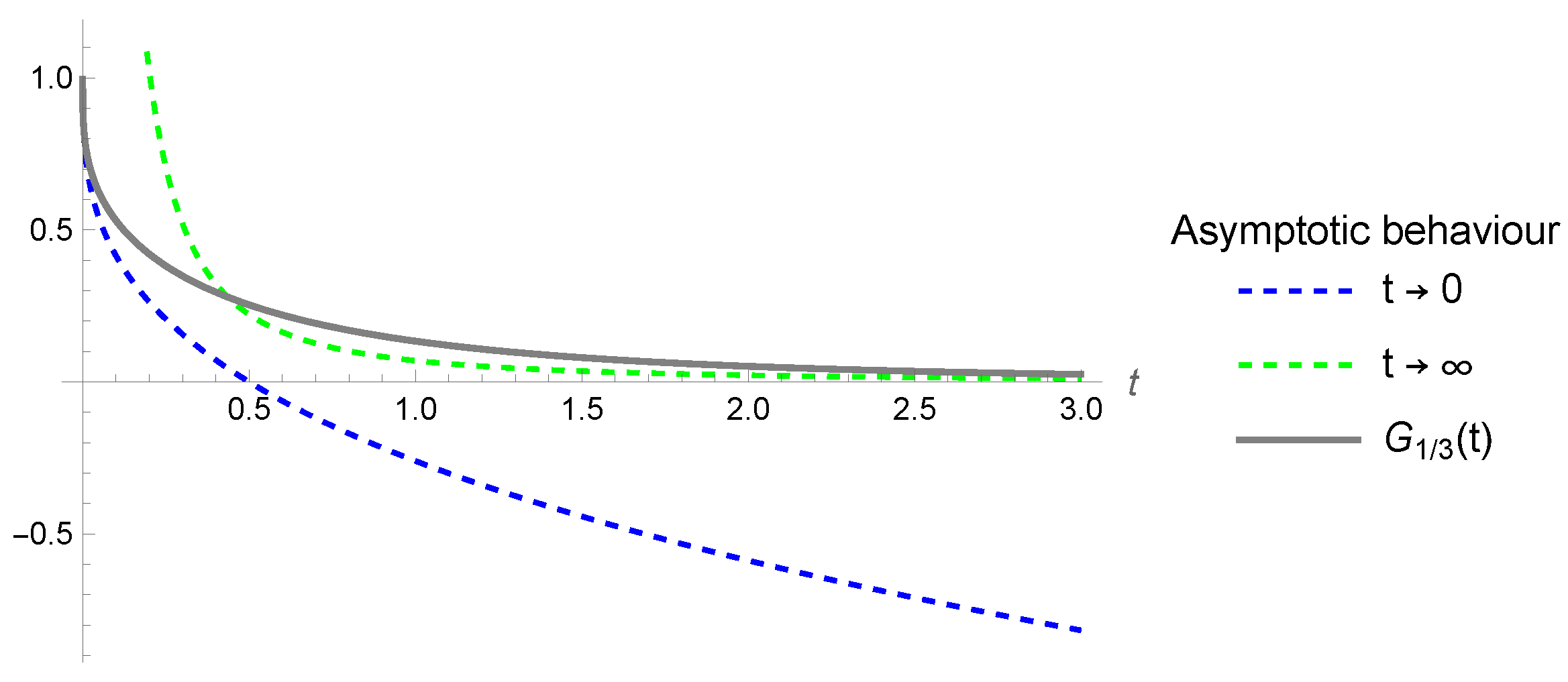
G 1 / 3 t 2 9 μ t τ 5 / 3 , t + .
As a consistency test, we can obtain (69) from the the expression given in (50) for G m / n t with m = 1 and n = 3 , and the asymptotic formula ([17] [Eqn. 18.1(22)]),
E α , β z k = 1 N z k Γ β α k + O z N , z , arg z < 1 α 2 π .

4.2. Asymptotic Behaviour for T 0 +

Rewrite the Laplace transform of the relaxation modulus (61), as follows:
G ˜ α s = μ s 1 1 + Γ α + 1 s τ α + s τ 1 .
Note that, for a 0 , 1 (thus 1 a 0 , 1 ), and A R , we have that
lim y + 1 + A y a + y 1 1 + A y a = lim y + y + A y 1 a + 1 y + A y 1 a = 1 ,
thus, taking A = Γ α + 1 , a = α 0 , 1 , and y = s τ + , (i.e., s + , since τ > 0 ), we get
1 + Γ α + 1 s τ α + s τ 1 1 + Γ α + 1 s τ α , s + .
Apply (73) to (71), in order to obtain
G ˜ α s μ s 1 1 + Γ α + 1 s τ α , s + .
Now, perform the change of variables x = 1 / z in (63),
1 1 + 1 z 1 1 z , z + ,
and take z = s τ α Γ α + 1 + (i.e., s + ), to arrive at
G ˜ α s μ 1 s Γ α + 1 τ α s α + 1 , s + .
According to (57), the asymptotic behaviour of G α t as t 0 + is calculated as
G α t μ L 1 1 s Γ α + 1 τ α s α + 1 ; t ,
i.e.,
G α t μ 1 t τ α , t 0 + .
Again, taking more terms in the expansion of G ˜ α s as s + , we can calculate more terms of G α t as t 0 + by using (57). Thereby, we obtain
G α t μ 1 t τ α + Γ 2 1 + α Γ 2 α 1 t τ 2 α + , t 0 + .
Note that the particular case α = 1 3 in (78) yields
G 1 / 3 t μ 1 t τ 1 / 3 , t 0 + .
As a consistency test, we can obtain (80) from the the expression given in (50) for G m / n t with m = 1 and n = 3 , and the definition of the Mittag–Leffler Function (45). Furthermore, the asymptotic formula given in (78) can be obtained from the Volterra integral Equation (4). Indeed, taking into account (2) and (3) and performing the change of variables x = t t , this integral equation reads as
G α t = μ 1 τ 0 t 1 + α t x τ α 1 G α x d x ,
thus,
lim t 0 + G α t = μ .
According to (82), we can take the approximation G α x μ as t 0 + in (81), thus
G α t μ μ τ 0 t 1 + α t x τ α 1 d x = μ 1 t τ t τ α
Recalling that α 0 , 1 , we recover (78), i.e.,
G α t μ 1 t τ α , t 0 + .
Figure 1 presents the graph of G 1 / 3 t for μ = 1 and different values of τ . Figure 2 shows the asymptotic behaviours given in (80) and (69) for G 1 / 3 t with μ = 1 and τ = 1 2 .

5. Numerical Results

5.1. Volterra Integral Equation

The quadrature formulas to numerically solve the Volterra integral equation [18] that satisfies G α t , i.e., Equation (81), fail because from (80), recalling that α 0 , 1 and μ , τ > 0 , we have that
lim t 0 + d G α t d t = .
However, we can apply a successive approximation method in order to numerically compute G α t ([19] [Sect. 2.1]). This method states that if we have the Volterra integral equation of the second kind
u t = f t + 0 t K x , t u x d x ,
we take as zeroth approximation
u 0 t = f t ,
and for the successive approximations j = 1 , 2 ,
u j t = f t + 0 t K x , t u j 1 x d x .
Figure 3 shows the application of this successive approximation method to the solution of (81) (i.e., taking as kernel K x , t = 1 τ 1 + α t x τ α 1 , and f t = μ in (86)), for μ = τ = 1 and α = 1 / 3 . It is apparent that as the order of approximation increases, we get a better approximation to the analytical solution G 1 / 3 t obtained in (37) or (54). Similar graphs are obtained for other rational values of α 0 , 1 compared to the analytical solution G α t obtained in (50).
Note that this successive approximation method has been successfully applied in Section 4 in order to derive the first order asymptotic formula (78).

5.2. Inverse Laplace Transform

According to our numerical experiments, the relative error between the analytical formulas of G α t and the numerical Laplace inversion of G ˜ α s , never exceeds the value of 10 9 in the time interval t 0 , 5 . Below we present some of these numerical experiments.
Figure 4 shows the relative error Δ MR t between G 1 / 3 MR t and G 1 / 3 num t , i.e., the numerical Laplace inversion of G ˜ 1 / 3 s using Talbot’s method [20],
Δ MR t = 1 G 1 / 3 MR t G 1 / 3 num t .
Figure 5 shows the relative error Δ R t between G 1 / 3 R t and G 1 / 3 num t ,
Δ R t = 1 G 1 / 3 R t G 1 / 3 num t .

6. Conclusions

Considering the Andrade model in linear viscoelasticity, we have derived for the first time an analytical expression for the relaxation modulus in the time domain G α t considering a rational parameter α 0 , 1 in terms of Mittag–Leffler functions (or equivalently, as a linear combination of Rabotnov functions). For the original parameter α = 1 / 3 of the Andrade model, we have derived a particular expression for G 1 / 3 t in terms of Miller-Ross functions. It turns out that this last expression is numerically more efficient (approximately twice faster) than the equivalent one in terms of Rabotnov functions.
Furthermore, we have obtained the asymptotic behaviour of G α t for t 0 + and t + using the Tauberian theorem. We have derived the same expression for the asymptotic behaviour as t 0 + by using the Volterra integral equation of the second kind that G α t satisfies.
Finally, numerical computations for particular values of the parameters have been performed in order to verify the analytical solutions obtained. For this purpose, we have used Talbot’s method for the numerical computation of the inverse Laplace transform, and the method of successive approximations for the numerical evaluation of the Volterra integral equation of the second kind.

Author Contributions

Conceptualization, G.S. and F.M.; methodology, J.L.G.-S. and A.A.; software, J.L.G.-S.; validation, J.L.G.-S. and A.A.; formal analysis, J.L.G.-S.; investigation, G.S.; writing—original draft preparation, J.L.G.-S.; writing—review and editing, G.S.; supervision, G.S. and A.A.; project administration, G.S. and F.M. All authors have read and agreed to the published version of the manuscript.

Funding

This research received no external funding.

Data Availability Statement

The original contributions presented in the study are included in the article, further inquiries can be directed to the corresponding author.

Conflicts of Interest

The authors declare no conflicts of interest.

References

  1. Christensen, R.M. Theory of Viscoelasticity; Courier Corporation: North Chelmsford, MA, USA, 2003. [Google Scholar]
  2. Andrade, E.N.D.C. On the viscous flow in metals, and allied phenomena. Proceedings of the Royal Society of London. Series A, Containing Papers of a Mathematical and Physical Character; Generic: Homebush West, NSW, Australia, 1910; Volume 84, pp. 1–12. [Google Scholar]
  3. Andrade, E.N.D.C. The validity of the t1/3 law of flow of metals. Philos. Mag. 1962, 7, 2003–2014. [Google Scholar] [CrossRef]
  4. Walterová, M.; Plesa, A.C.; Wagner, F.W.; Breuer, D. Andrade Rheology in Planetary Science. Authorea Preprints. 2023. Available online: https://essopenarchive.org/doi/full/10.22541/essoar.169008299.99203183 (accessed on 25 July 2024).
  5. Rosti, J.; Koivisto, J.; Laurson, L.; Alava, M. Fluctuations and scaling in creep deformation. Phys. Rev. Lett. 2010, 105, 100601. [Google Scholar] [CrossRef] [PubMed]
  6. Pandey, V. Hidden jerk in universal creep and aftershocks. Phys. Rev. 2023, 107, L022602. [Google Scholar] [CrossRef] [PubMed]
  7. Bagheri, A.; Khan, A.; Al-Attar, D.; Crawford, O.; Giardini, D. Tidal response of Mars constrained from laboratory-based viscoelastic dissipation models and geophysical data. J. Geophys. Res. Planets 2019, 124, 2703–2727. [Google Scholar] [CrossRef]
  8. Castillo-Rogez, J.C.; Efroimsky, M.; Lainey, V. The tidal history of Iapetus: Spin dynamics in the light of a refined dissipation model. J. Geophys. Res. Planets 2011, 116, E09008. [Google Scholar] [CrossRef]
  9. Mainardi, F. Fractional Calculus and Waves in Linear Viscoelasticity: An Introduction to Mathematical Models; World Scientific: Singapore, 2022. [Google Scholar]
  10. Mainardi, F.; Spada, G. On the viscoelastic characterization of the Jeffreys–Lomnitz law of creep. Rheol. Acta 2012, 51, 783–791. [Google Scholar] [CrossRef]
  11. Cosorzi, A.; Mellini, D.; González-Santander, J.; Spada, G. On the Love numbers of an Andrade planet. Earth Space Sci. 2024. [Google Scholar]
  12. Apelblat, A. Laplace Transforms and Their Applications; Mathematics Research Developments Series; Nova Science Publishers: Hauppauge, NY, USA, 2012. [Google Scholar]
  13. Prudnikov, A.P.; Brychkov, Y.A.; Marichev, O.I. Integrals and Series: Inverse Laplace Transforms; CRC Press: Boca Raton, FL, USA, 1986; Volume 5. [Google Scholar]
  14. Olver, F.W.J.; Lozier, D.W.; Boisvert, R.F.; Clark, C.W. NIST Handbook of Mathematical Functions; Cambridge University Press: Cambridge, UK, 2010. [Google Scholar]
  15. Oldham, K.B.; Myland, J.; Spanier, J. An Atlas of Functions: With Equator, the Atlas Function Calculator; Springer: Berlin/Heidelberg, Germany, 2009. [Google Scholar]
  16. Sandev, T.; Tomovski, Z. Fractional equations and models. In Theory and Applications; Springer Nature Switzerland AG: Cham, Switzerland, 2019. [Google Scholar]
  17. Erdélyi, A.; Magnus, W.; Oberhettinger, F.; Tricomi, F.G. Higher Transcendental Functions; McGraw-Hill: New York, NY, USA, 1955; Volume 3. [Google Scholar]
  18. Rakotch, E. Numerical solution of Volterra integral equations. Numer. Math. 1972, 20, 271–279. [Google Scholar] [CrossRef]
  19. Tricomi, F.G. Integral Equations; Courier Corporation: North Chelmsford, MA, USA, 1985; Volume 5. [Google Scholar]
  20. Talbot, A. The accurate numerical inversion of Laplace transforms. IMA J. Appl. Math. 1979, 23, 97–120. [Google Scholar] [CrossRef]
Figure 1. Graph of G 1 / 3 t for μ = 1 .
Fractalfract 08 00439 g001
Figure 2. Asymptotic behaviour of G 1 / 3 t for μ = 1 and τ = 1 2 .
Fractalfract 08 00439 g002
Figure 3. Successive approximations G 1 / 3 j t for μ = τ = 1 .
Fractalfract 08 00439 g003
Figure 4. Graph of Δ MR t for μ = τ = 1 .
Fractalfract 08 00439 g004
Figure 5. Graph of Δ R t for μ = τ = 1 .
Fractalfract 08 00439 g005
Disclaimer/Publisher’s Note: The statements, opinions and data contained in all publications are solely those of the individual author(s) and contributor(s) and not of MDPI and/or the editor(s). MDPI and/or the editor(s) disclaim responsibility for any injury to people or property resulting from any ideas, methods, instructions or products referred to in the content.