Article

Volatility Analysis of Financial Time Series Using the Multifractal Conditional Diffusion Entropy Method

1
Department of Mathematical Sciences, University of Texas at El Paso, El Paso, TX 79968, USA
2
Department of Computational Science, University of Texas at El Paso, El Paso, TX 79968, USA
3
Department of Data Science, Ramapo College of New Jersey, Mahwah, NJ 07430, USA
*
Author to whom correspondence should be addressed.
Fractal Fract. 2024, 8(5), 274; https://doi.org/10.3390/fractalfract8050274
Submission received: 30 January 2024 / Revised: 30 April 2024 / Accepted: 30 April 2024 / Published: 4 May 2024

Abstract

:
In this article, we introduce the multifractal conditional diffusion entropy method for analyzing the volatility of financial time series. This method utilizes a q-order diffusion entropy based on a q-weighted time lag scale. The technique of conditional diffusion entropy proves valuable for examining bull and bear behaviors in stock markets across various time scales. Empirical findings from analyzing the Dow Jones Industrial Average (DJI) indicate that employing multi-time lag scales offers greater insight into the complex dynamics of highly fluctuating time series, often characterized by multifractal behavior. A smaller time scale like t = 2 to t = 256 coincides more with the state of the DJI index than larger time scales like t = 256 to t = 1024 . We observe extreme fluctuations in the conditional diffusion entropy for DJI for a short time lag, while smoother or averaged fluctuations occur over larger time lags.

1. Introduction

Practitioners, researchers, and regulators across the domains of economics, mathematics, and physics increasingly prioritize understanding the stability of financial systems in response to the subprime crisis [1]. This heightened importance extends to asset and derivative pricing, asset allocation, and risk management. Concepts and techniques derived from complex systems and econophysics drive investigations into anomalous, chaotic, and non-stationary behavior within economic systems, with entropy playing a crucial role. The literature abounds with examples showcasing abrupt transitions from stable states to radically different ones, building upon prior studies that frame the financial crisis as a complex dynamical system.
In [2], the authors focus on examining scaling and memory phenomena within the context of return intervals associated with stock and currency data. Their findings reveal that a singular scaling function can effectively approximate the distribution function of return intervals. Furthermore, the study underscores robust memory effects, indicating that shorter return intervals are more likely to succeed other short intervals. In contrast, longer intervals tend to be followed by similarly extended periods.
Siokis (2012) analyzes the distribution of the magnitude of significant stock market shocks [3]. The study models the behavior of market index returns before and after significant crashes, aiming to identify statistical patterns. The analysis reveals that, for a considerable number of market crashes, the distribution of market volatility before and after the crash follows the Gutenberg-Richter law, signifying the presence of scale-invariance and self-similarity in the underlying dynamics through a robust power-law relationship.
In [4], Wang et al. examine volatility return intervals for the most heavily traded stocks in the United States markets. The study reveals that the scaling exponent exhibits dependence on the threshold value q, indicating the presence of a multiscaling nature in the distribution of return intervals. They delve into the multiscaling exponent, which characterizes the multiscaling behavior of individual stocks.
The author in [5] investigates the impact of an entropy disturbance in the United States on the entropy levels of other financial markets by employing singular value decomposition on the constituents of stock market indices from different economies.
In [6], the author discusses whether uncertainty and disorder in the stock market reflect entropy. In [7], the authors investigate the volatility of seven stock market indices based on Tsallis and Shannon entropy. Compared to other methods, such as convexity, variance, and vector autoregression (VaR), the authors in [8] find that the information entropy method is a better way to quantify the risk associated with bonds. Therefore, identifying potentially significant factors to reduce the negative consequences on economic systems has received attention recently, even though global financial crises usually result from events generated in the financial industry sectors.
This study aims to extend the Conditional Diffusion Entropy Analysis developed in [9,10] to a Multi-scale Conditional Diffusion Entropy (MS-CDE) as another pertinent method. Our proposed model serves as the multifractal extension of the CDE. It emphasizes the role of Shannon entropy (SE) and Rényi entropy (RE). The monofractal approach utilizes the SE of Scafetta et al. [11] while the multifractal approach employs a combination of SE and RE for different q weights to estimate scaling exponents [12,13]. The study proposes the examination of bull and bear markets using multi-time lag scales to determine MS-CDE. It leverages the study on optimal bin-width in empirical histograms by Jizba et al. [14] to evaluate the underlying probability density function (PDF).
This paper presents the following structure: Section 2 briefly reviews the foundations of the diffusion entropy analysis (DEA) required for determining CDE and MS-CDE. We also provide a brief overview of the q-order DEA, which facilitates the calculation of MS-CDE. Section 3 introduces the time series from the DJI market index sampled daily from April 2013 to April 2021, which we use to generate empirical results. Section 4 showcases the results from the experiment, and corresponding discussions occur in Section 5. Finally, Section 6 concludes the paper.

2. Methodology

2.1. Diffusion Entropy Analysis (DEA)

Let N be the length of a financial time series { Y i } i = 1 N . The process is as follows [11].
  • Transform the series { Y i } i = 1 N into a diffusion process. Consider the series such that it can be written as:
    { Y i , Y i + 1 , Y i + 2 , , Y i + t 1 }
    where i = 1 , 2 , , N t + 1 and t [ 1 , N ] is the time scale. The matrix ψ i j defined as
    ψ i j = Y i + j Y i + j 1 , j = 0 , 1 , , N t
    can be regarded as sub-sequences for any given diffusion time t with initial state ψ i 0 = 0 . Next, construct a diffusion trajectory for each of these sub-sequences using the stochastic process
    η t j = i = 1 t ψ i j ,
    where η t j is the new position of the jth particle in the diffusion process.
  • Compute the diffusion entropy. First, partition the x-axis into bin size B ( t ) and assume that N i ( t ) represents the number of particles falling in each bin at time t where i = 1 , 2 , , B ( t ) .
  • Determine the optimal bin size B. We note that there is no “best” number of bins, and different bin sizes B reveal different data features. Wider bins are utilized when the density of the underlying data points is low, reducing sampling-related noise. Conversely, narrower bins are employed when the density is high, enhancing the precision of density estimation. Hence, it proves advantageous to adjust the bin size within a histogram. For our calculations, we utilize the Freedman-Diaconis’ rule [15] to determine the bin size B, which is defined as:
    B = 2 Interquartile range n 3 .
    Freedman-Diaconis’ rule is less sensitive to outliers in data compared to the standard deviation, rendering it more robust. Another approach is the Scott’s rule [16]. It is defined as B = 3.5 σ ^ n 3 , where σ ^ denotes the sample standard deviation. Scott’s rule works best with data that follows a Gaussian distribution.
  • We approximate the probability density function (PDF) of a particle falling into a bin at time t using the relative frequency as:
    p ( i , t ) = N i ( t ) N t + 1 .
    At each time t, we calculate the diffusion (Shannon) entropy as follows:
    S ( t ) = i = 1 B ( t ) p ( i , t ) l n [ p ( i , t ) ] .
    Normalizing the diffusion entropy at time t results in:
    S ¯ ( t ) = S ( t ) t .
We obtain the linear-log relationship between entropy S ( t ) and time t [17,18] as:
S ( t ) = A + δ l n ( t ) .

2.2. Conditional Diffusion Entropy (CDE)

Conditional Diffusion Entropy, C ( t ) , provides a framework for distinguishing between bear and bull markets. In a bull market, the market expands, and economic conditions are typically favorable. In contrast, a bear market develops when the economy contracts and most stocks and equities lose value. The CDE, C ( t ) , as shown in [9,10], is defined as:
C ( t ) = 1 + α [ 1 S ¯ ( t ) ] .
Here, S ¯ ( t ) is the normalized entropy as shown in Equation (6). The coefficient α is defined by:
α = 1 , p < q 0 , p = q 1 , p > q .
In Equation (9), p and q denote the number of negative and positive values in the series, respectively. Thus, during a bear market, α > 0 , while during a bull market, α < 0 . When the market is indifferent or random, α = 0 , indicating neither a bull nor a bear market.

2.3. q-Order Diffusion Entropy Analysis (Q-DEA)

As multifractality presents a continuous property of time series, techniques that address problems concerning discretization and finite size of histograms employ interpolation approaches, rendering them susceptible to bias. When determining the optimal bin size B for different values of q, the Rényi entropy incorporates both the probabilities p i and their q-th powers p i q for different q. The q-order Scott’s rule for determining bin size B q is given as:
B q = ( 24 π ) 1 / 3 q 2 q 1 6 k = 1 m σ s k 2 ( 1 q ) / N s k k = 1 m σ s k ( 1 + 2 q ) 1 / 3 ,
where q = 0 , 1 , 2 , 3 , 4 and scale s k = 2 k ,   k = 1 , 2 , 3 , , m = f l o o r ( log N ) .
We substitute the theoritical standard deviation σ with the empirical standard deviation σ ^ to get
B q ^ = ( 24 π ) 1 / 3 q 2 q 1 6 k = 1 m σ ^ s k 2 ( 1 q ) / N s k k = 1 m σ ^ s k ( 1 + 2 q ) 1 / 3 .
( 24 π ) 1 / 3 q 2 q 1 6 N q , m σ ^ ,
where
N q , m σ ^ = k = 1 m σ ^ s k 2 ( 1 q ) / N s k k = 1 m σ ^ s k ( 1 + 2 q ) 1 / 3 .
For Freedman-Diaconis’ rule, replace the estimated standard deviation with the IQR to get
B q ^ = 2.6 q 2 q 1 6 N q , m I Q R ^ .
Please see the reference [14] for more details.
To analyze multifractal scaling properties of a time series, we use the q-order entropy, which is a family of Shannon and Rényi entropies defined as:
S q ( t ) = i = 1 B q ( t ) p ( i , t ) l n [ p ( i , t ) ] , q = 1 1 1 q l n i = 1 B q ( t ) p q ( i , t ) , q 1 , q R + .
Here, q R + denotes the weight assigned to different probabilities of a particle falling in a bin. We constrain q 0 because information extraction is compromised for q < 0 [19]. This method is called the multifractal diffusion entropy analysis (MFDEA). The DEA corresponds to the q-order DEA where q = 1 . We express the linear-log relationship between the q-order diffusion entropy S q ( t ) and time t as:
S q ( t ) = A + δ q l n ( t ) .

2.4. Multi-Scale Conditional Diffusion Entropy (MS-CDE)

The q-order Conditional Diffusion Entropy (MS-CDE) serves as the multifractal extension of the CDE, offering a means to distinguish between bear and bull situations in the market at various q -weights, representing different probabilities of a particle falling in a bin. MS-CDE is defined as:
C q ( t ) = I + α [ I S ¯ q ( t ) ] ,
where I is a vector of ones and S ¯ q ( t ) is the q-order vector of normalized entropy from Equation (12) and
α = 1 , p < q 0 , p = q 1 , p > q .

3. Data

Table 1 displays the start-date and end-date of data used in this paper. We adopt the daily close prices of the Dow Jones Industrial Average (DJI) from April 2013 to April 2021, amounting to 2028 data points. As illustrated in Figure 1, market prices tend to fall during a financial crisis, while they rise during the market recovery period following a crisis. The highlighted portion of the graph in Figure 1 indicates the crash.

4. Results

In this section, we present results by examining the stock market’s stability during the COVID-19 pandemic stock market crash using the multi-scale conditional diffusion entropy. The analyzed crash period is highlighted in Figure 1.

4.1. q-Order DEA for Dow Jones Industrial Average

Figure 2 below shows a plot of diffusion entropy versus scale for q weighted in the range 0 to 4 for DJI from April 2013 to April 2021. At certain diffusion times t, entropy decreases with the increase in q weights, whereas entropy increases with the rise in q weights at other diffusion times. This phenomenon occurs because the Rényi entropy changes more rapidly at large q than small q weights.

4.2. Multi-Scale Conditional Entropy of DJI from April 2013 to April 2021

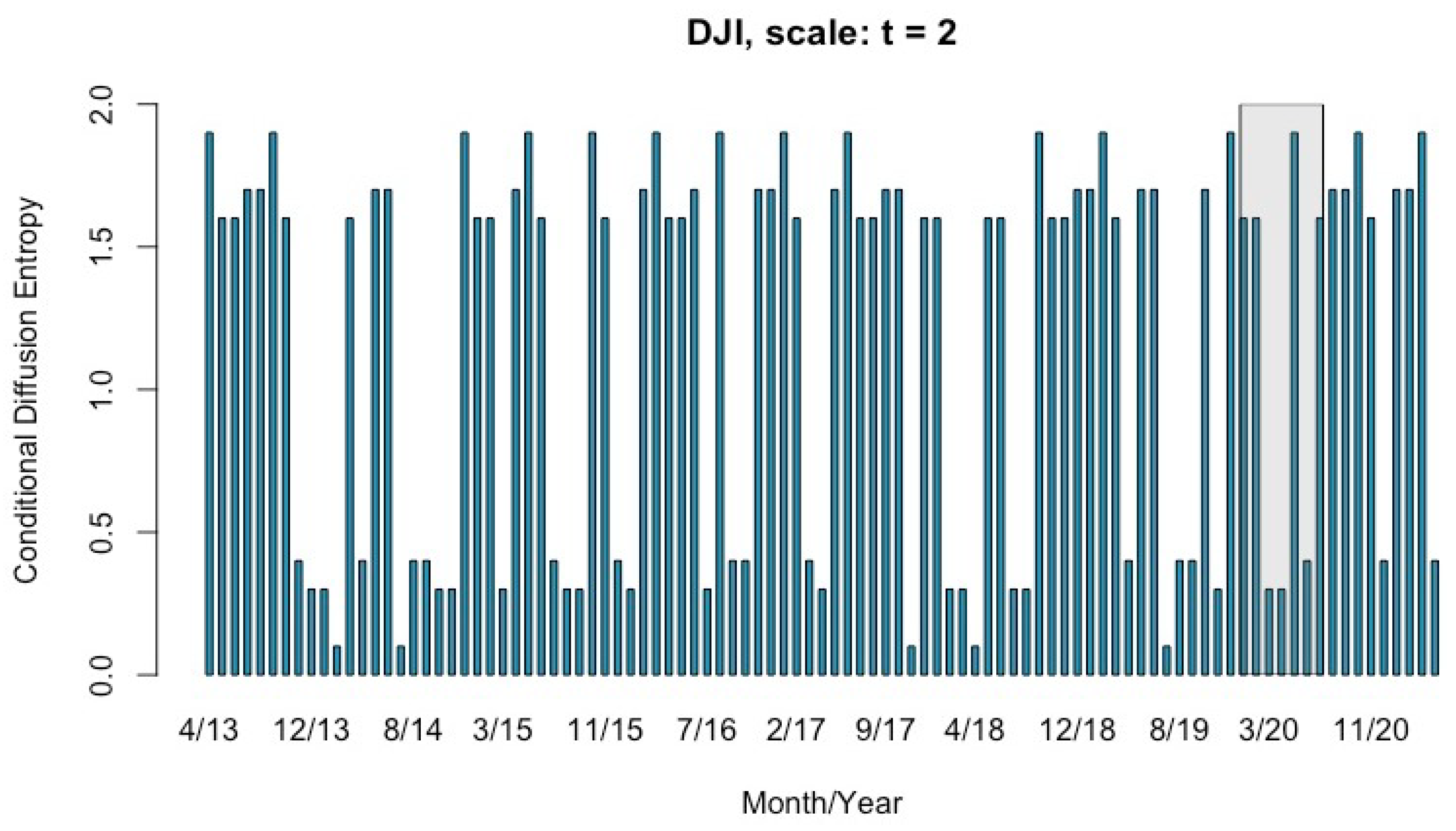
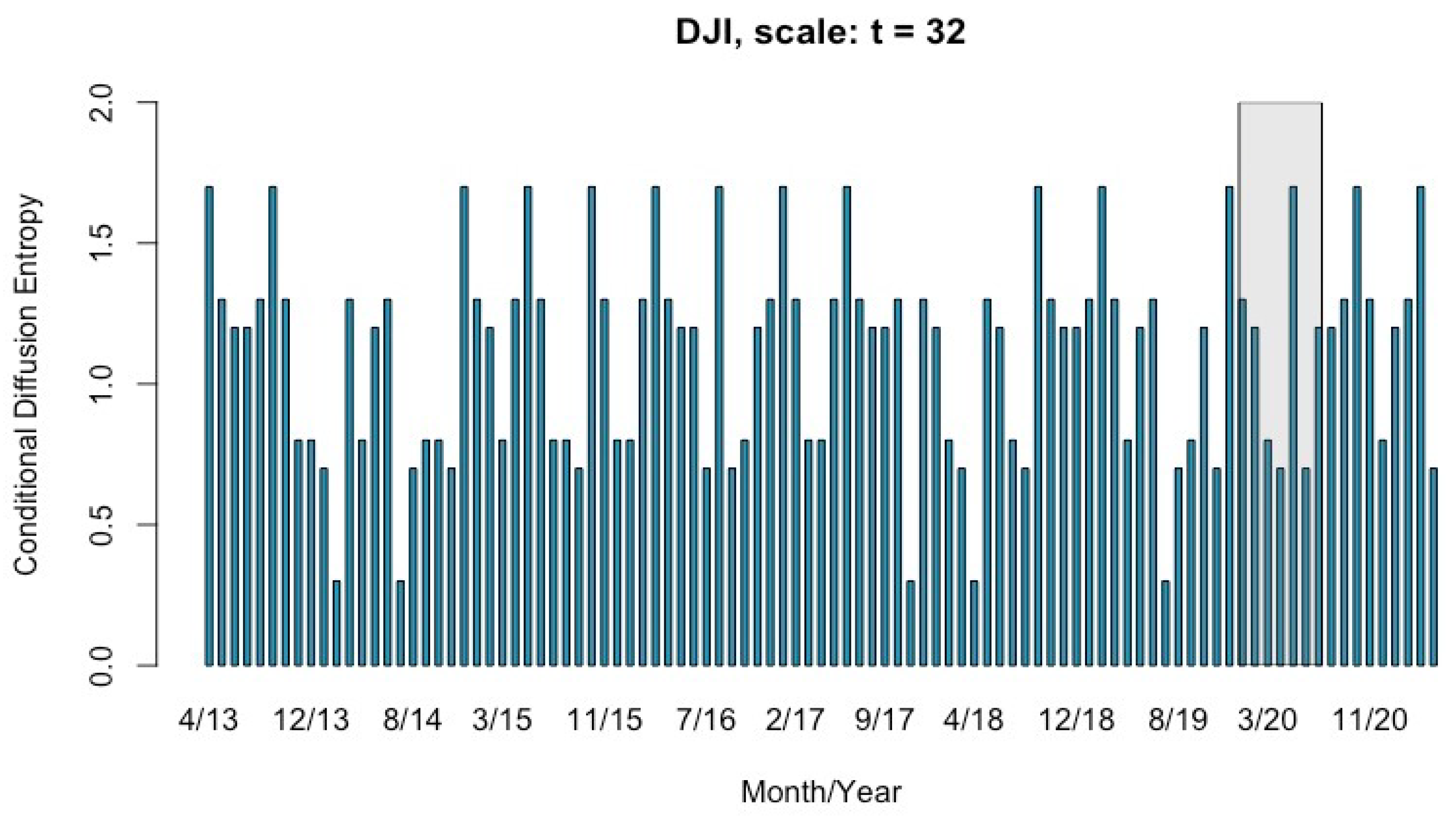
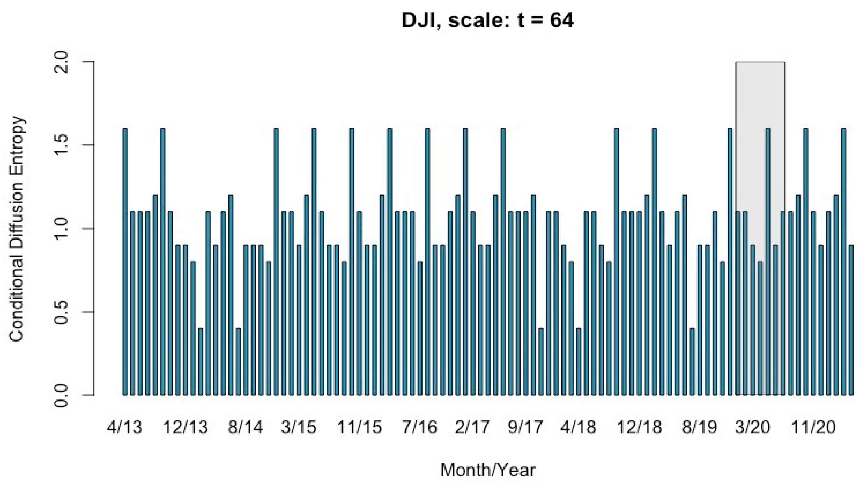
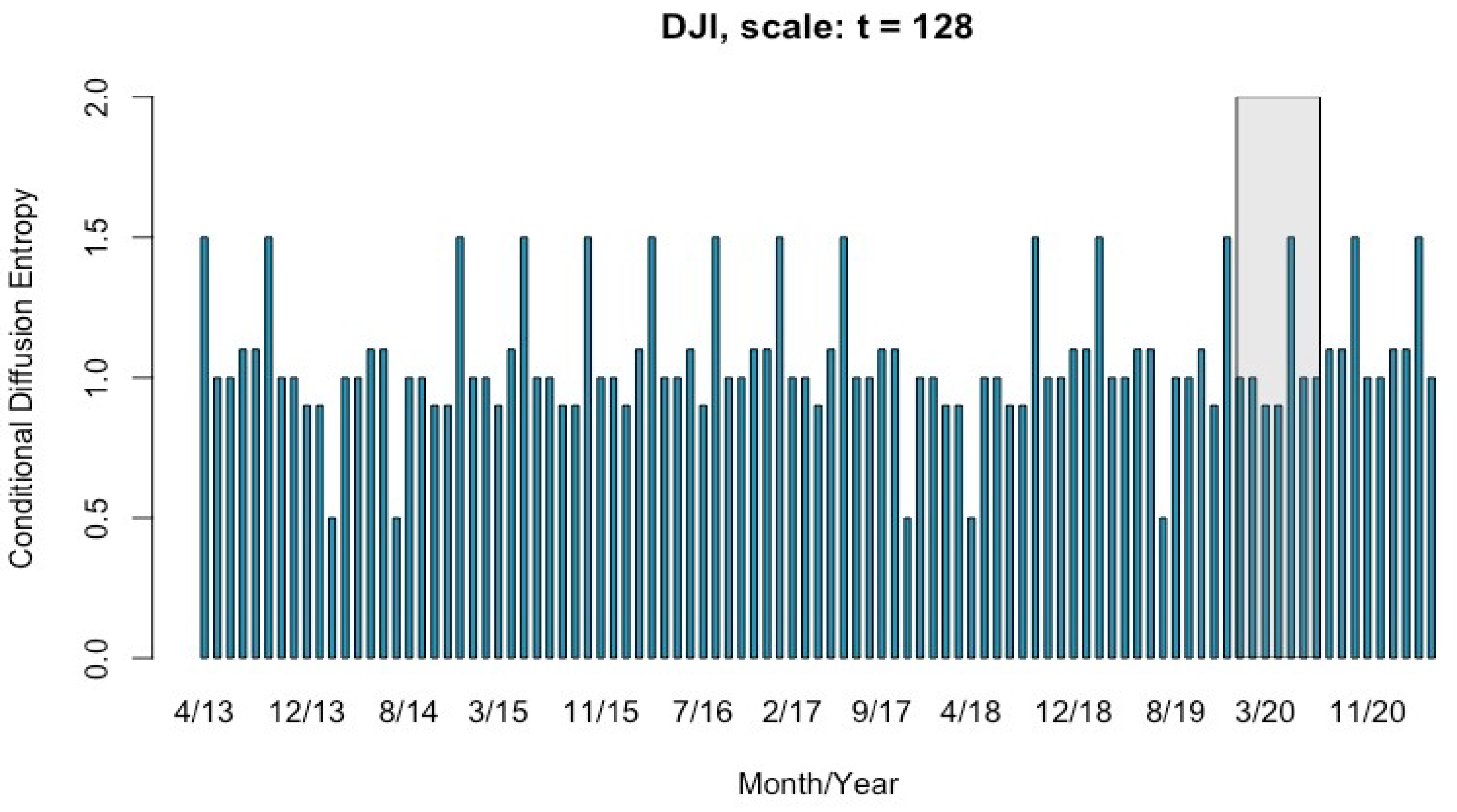
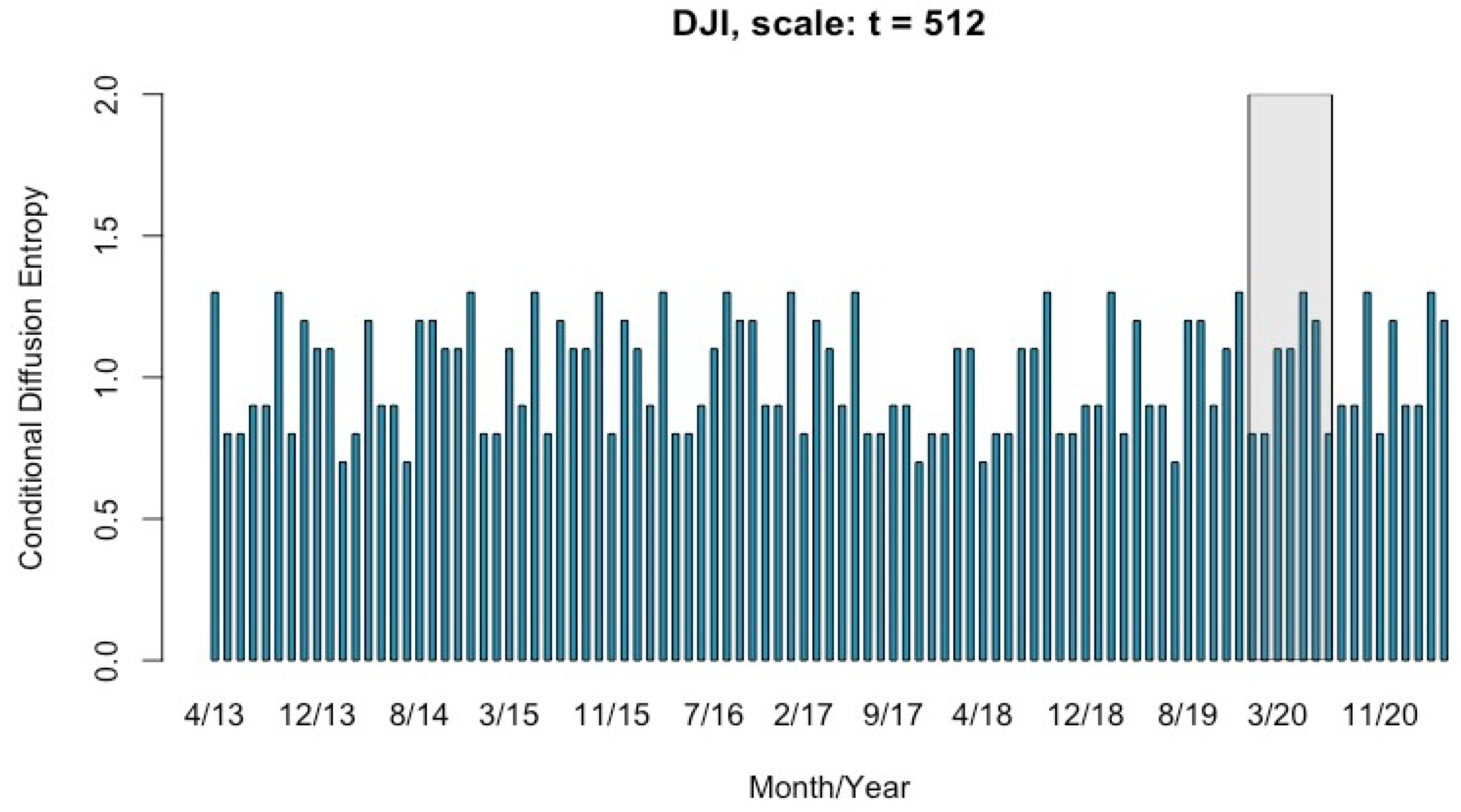
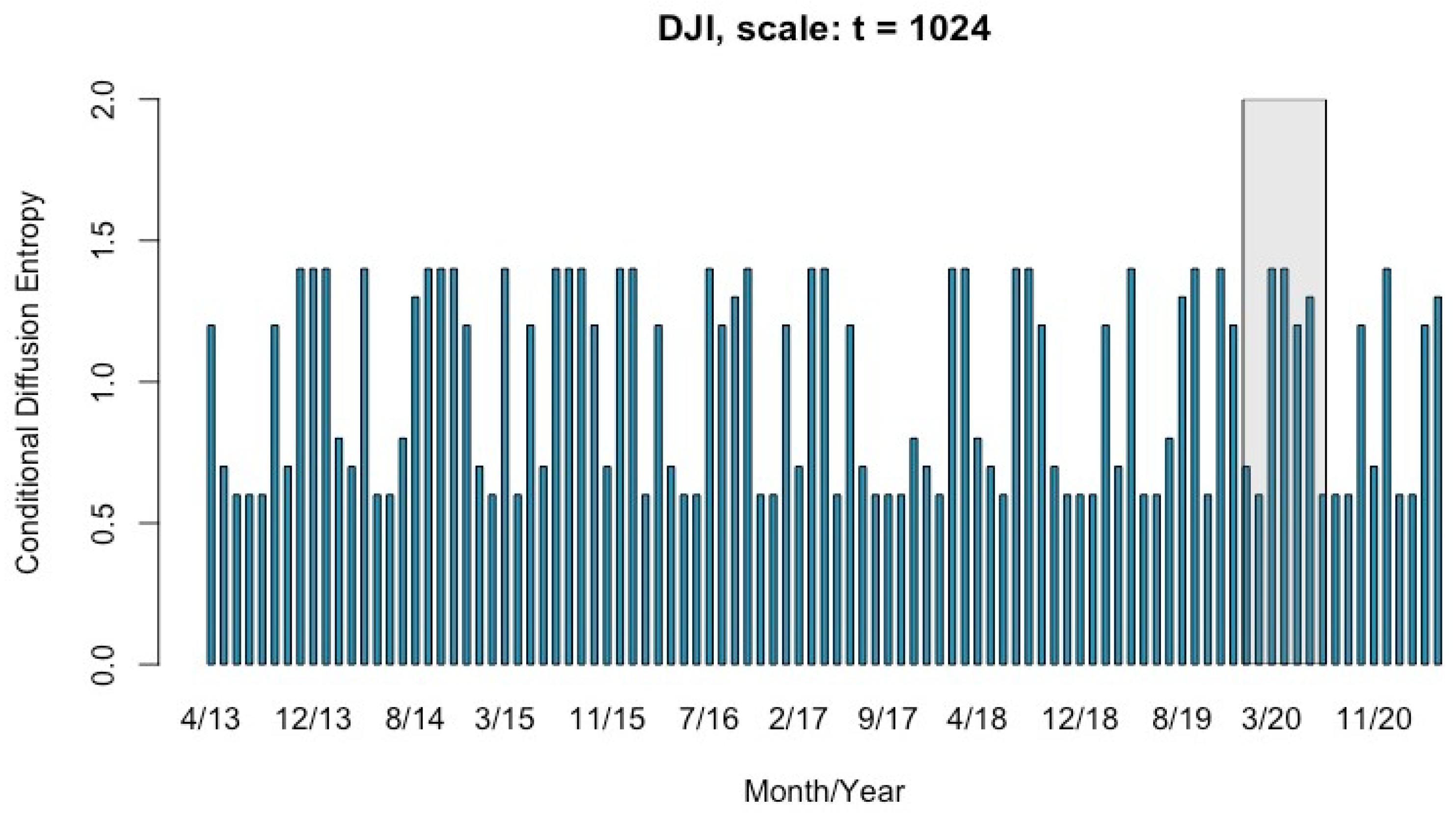
Figure 3, Figure 4, Figure 5, Figure 6, Figure 7, Figure 8, Figure 9, Figure 10, Figure 11 and Figure 12 show the monthly conditional diffusion entropy C q ( t ) at different time scales from April 2013 to April 2021. In this representation, C q ( t ) = 1 signifies random behavior in the financial market, C q ( t ) > 1 indicates a bull market, and values less than 1 denote a bear market.

5. Discussion

Figure 1 displays instances of bull and bear markets in the DJI index. The highlighted portion represents the period from late February 2020 to early April 2020, depicting the 2020 coronavirus stock market crash. During this period, the COVID-19 pandemic spread globally from February 24 to 28, causing a significant decline in global stock markets. The DJI drops 11–12%, marking the most significant weekly decline since the 2007/2008 financial crisis. On March 12, a day after the announcement of a travel ban from Europe, the DJI fell sharply again by 10%. After it became clear that a recession was inevitable, the DJI dropped another 12.93% on March 16. Stock market indices briefly recover to their levels at the end of February 2020 by early June 2020.
Figure 1 shows the fluctuations in the series over time. Many values of the conditional diffusion entropy at time scale t = 2 are larger than 1 during bull market periods. In contrast, they are less than 1 during periods of the financial crisis (or bear market), as shown by the grey highlighted part of Figure 3. Observe that, as the time scale increases from t = 2 to t = 256 , the conditional diffusion entropy approach is a random behavior where most of the C q ( t ) 1 as shown in Figure 4, Figure 5, Figure 6, Figure 7, Figure 8, Figure 9 and Figure 10. During this period, the market is indifferent. Beyond the time scale of t = 256 , conditional diffusion entropy is less than 1, as shown in Figure 11 and Figure 12, indicating that the bear market is dominant. Hence, the conditional diffusion entropy value coincides with the state of the stock market but at different time lags, and the conditional diffusion entropy depicts the various states of the stock market. A smaller time scale like t = 2 to t = 256 coincides more with the state of the stock market than larger time scales like t = 256 to t = 1024 . This is because we observe extreme fluctuations in the conditional diffusion entropy for a short time lag. In contrast, smoother (or averaged-out) fluctuations are observed in larger time scales, resulting in lower values of the conditional diffusion entropy. Comparing the Conditional Diffusion Entropy method developed in [9,10] to our model’s results, we observe that Multiscale Conditional Diffusion Entropy Analysis is less prone to incorrectly classifying a bullish market as neutral or bearish. This is because MS-CDE assesses market volatility across multiple time scales, unlike CDE. Thus, MS-CDE conditional diffusion offers a more insightful analysis of stock market volatility. However, one limitation of using MS-CDE is its computational intensity, which is due to the use of multiple time scales in our analysis.

6. Conclusions

This paper investigates the stability of the Dow Jones Industrial Average (DJI) in the US stock markets utilizing multi-scale normalized and conditional diffusion entropy. We discover that conditional diffusion entropy is valuable for analyzing market fluctuations and discerning bear and bull markets. However, careful interpretation of its results is necessary. We illustrate that conditional diffusion entropy offers diverse insights into the market’s state at different time lag scales. Hence, employing a multi-time lag scale enhances the analysis of financial market time series, especially considering their often multifractal nature. As a future direction, we plan to extend our inquiry to volatility in other financial securities, such as bonds and cryptocurrency markets, using our innovative approach. Moreover, implementing the method in parallel will mitigate the computational intensity of the model. Additionally, we aim to compare our technique with other multiscale techniques like the wavelet approach or scale-space filtering.

Author Contributions

Conceptualization, W.K., M.C.M. and O.K.T.; methodology, M.C.M., W.K., P.K.A. and O.K.T.; software, W.K.; validation, O.K.T.; formal analysis, W.K.; data curation, W.K. and P.K.A.; writing—original draft preparation, W.K.; writing—review and editing, O.K.T.; visualization, W.K.; supervision, M.C.M. and O.K.T. All authors have read and agreed to the published version of the manuscript.

Funding

This research received no external funding.

Data Availability Statement

The raw data supporting the conclusions of this article will be made available by the authors on request.

Conflicts of Interest

The authors declare no conflict of interest.

Abbreviations

List of Acronyms.
AcronymsDefinition
DJIDow Jones Industrial Average
SEShannon Entropy
RERényi Entropy
VaRVector Autoregression
CDEConditional Diffusion Entropy
MS-CDEMulti-Scale Conditional Diffusion Entropy
PDFProbability Density Function
DEADiffusion Entropy Analysis
FDFreedman-Diaconis Rule
Q-DEAq-Order Diffusion Entropy Analysis
IQRInter quartile Range
MFDEAMultifractal Diffusion Entropy Analysis

References

  1. Andreev, B.; Sermpinis, G.; Stasinakis, C. Modelling Financial Markets during Times of Extreme Volatility: Evidence from the GameStop Short Squeeze. Forecasting 2022, 4, 654–673. [Google Scholar] [CrossRef]
  2. Yamasaki, K.; Muchnik, L.; Havlin, S.; Bunde, A.; Stanley, H.E. Scaling and memory in volatility return intervals in financial markets. Proc. Natl. Acad. Sci. USA 2005, 102, 9424–9428. [Google Scholar] [CrossRef] [PubMed]
  3. Siokis, F.M. Stock market dynamics: Before and after stock market crashes. Physica A 2012, 391, 1315–1322. [Google Scholar] [CrossRef]
  4. Wang, F.; Yamasaki, K.; Havlin, S.; Stanley, H.E. Multifactor analysis of multiscaling in volatility return intervals. Phys. Rev. E 2009, 79, 016103. [Google Scholar] [CrossRef] [PubMed]
  5. Caraiani, P. Modeling the Comovement of Entropy between Financial Markets. Entropy 2018, 20, 417. [Google Scholar] [CrossRef] [PubMed]
  6. McCauley, J.L. Thermodynamic analogies in economics and finance: Instability of markets. Physica A 2003, 329, 199–212. [Google Scholar] [CrossRef]
  7. Bentes, S.R.; Menezes, R. Entropy: A new measure of stock market volatility? J. Phys. Conf. Ser. 2012, 394, 012033. [Google Scholar] [CrossRef]
  8. Zhou, R.; Zhang, J.; Xiong, M.; Yang, F.; Yu, M. Using information entropy to measure bond risk: An empirical investigation. J. Inf. Comput. Sci. 2015, 12, 1089–1100. [Google Scholar] [CrossRef]
  9. Oh, G.; Kim, H.Y.; Ahn, S.W.; Kwak, W. Analyzing the financial crisis using the entropy density function. Phys. A Stat. Mech. Its Appl. 2015, 419, 464–469. [Google Scholar] [CrossRef]
  10. Li, S.; Zhuang, Y.; He, J. Stock market stability: Diffusion Entropy Analysis. Phys. A Stat. Mech. Its Appl. 2016, 450, 462–465. [Google Scholar] [CrossRef]
  11. Scafetta, N.; Grigolini, P. Scaling detection in time series: Diffusion entropy analysis. Phys. Rev. E Stat. Nonlinear Softw. Matter. Phys. 2002, 66, 036130. [Google Scholar] [CrossRef]
  12. Huang, J.; Shang, P.; Zhao, X. Multifractal diffusion entropy analysis on stock volatility in financial markets. Physica A 2012, 391, 5739–5745. [Google Scholar] [CrossRef]
  13. Morozov, A.Y. Comment on ’multifractal diffusion entropy analysis on stock volatility in financial markets’ [Physica A. 391 (2012) 5739–5745]. Physica A 2012, 392, 2442. [Google Scholar] [CrossRef]
  14. Jizba, P.; Korbel, J. Multifractal diffusion entropy analysis: Optimal bin width of probability histograms. Phys. A Stat. Mech. Its Appl. 2014, 413, 438–458. [Google Scholar] [CrossRef]
  15. Freedman, D.; Diaconis, P. On the histogram as a density estimator: L2 theory. Z. Wahrscheinlichkeitstheorie Verwandte Geb. 1981, 57, 453–476. [Google Scholar] [CrossRef]
  16. Scott, D.W. On optimal and data-based histograms. Biometrika 1979, 66, 605–610. [Google Scholar] [CrossRef]
  17. Mariani, M.C.; Kubin, W.; Asante, P.K.; Tweneboah, O.K.; Beccar-Varela, M.P.; Jaroszewicz, S.; Gonzalez-Huizar, H. Self-Similar Models: Relationship between the Diffusion Entropy Analysis, Detrended Fluctuation Analysis and Lévy Models. Mathematics 2020, 8, 1046. [Google Scholar] [CrossRef]
  18. Mariani, M.C.; Asante, P.K.; Bhuiyan, M.A.M.; Beccar-Varela, M.P.; Jaroszewicz, S.; Tweneboah, O.K. Long-Range Correlations and Characterization of Financial and Volcanic Time Series. Mathematics 2020, 8, 441. [Google Scholar] [CrossRef]
  19. Jizba, P.; Arimitsu, T. The world according to Rényi: Thermodynamics of multifractal systems. Ann. Phys. 2004, 312, 17–59. [Google Scholar] [CrossRef]
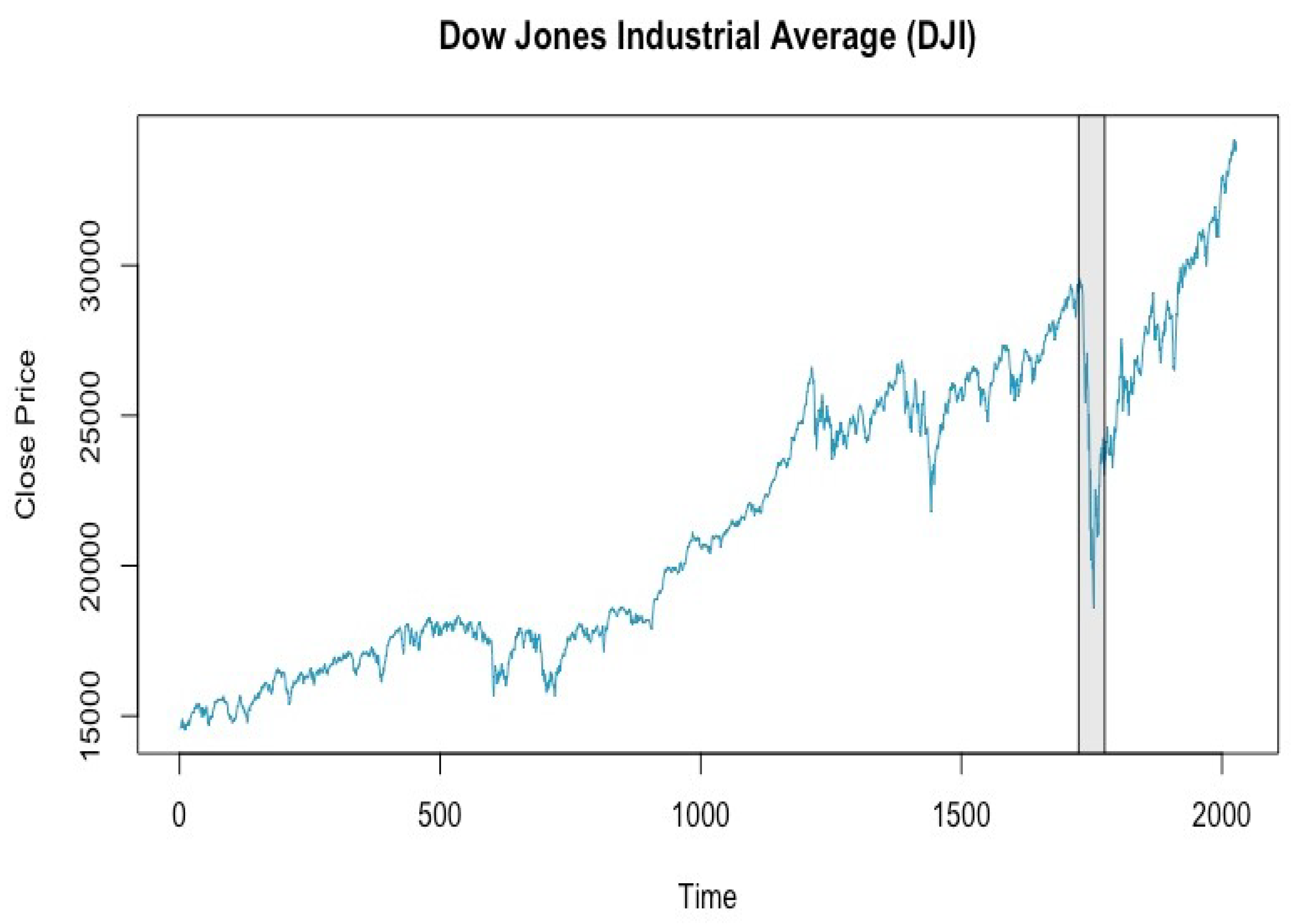
Figure 1. Daily Close Prices Plot of DJI. The grey area corresponds to a period of a financial crash.
Fractalfract 08 00274 g001
Figure 2. q-order Diffusion Entropy as a function of diffusion time constructed based on different q values of Rényi family of entropies using DJI.
Fractalfract 08 00274 g002
Figure 3. Monthly Conditional Entropy of DJI at Different Time Scales. The grey area are periods of the financial crisis (or bear market).
Fractalfract 08 00274 g003
Figure 4. Monthly Conditional Entropy of DJI at Different Time Scales. The grey area are periods of the financial crisis (or bear market).
Fractalfract 08 00274 g004
Figure 5. Monthly Conditional Entropy of DJI at Different Time Scales. The grey area are periods of the financial crisis (or bear market).
Fractalfract 08 00274 g005
Figure 6. Monthly Conditional Entropy of DJI at Different Time Scales. The grey area are periods of the financial crisis (or bear market).
Fractalfract 08 00274 g006
Figure 7. Monthly Conditional Entropy of DJI at Different Time Scales. The grey area are periods of the financial crisis (or bear market).
Fractalfract 08 00274 g007
Figure 8. Monthly Conditional Entropy of DJI at Different Time Scales. The grey area are periods of the financial crisis (or bear market).
Fractalfract 08 00274 g008
Figure 9. Monthly Conditional Entropy of DJI at Different Time Scales. The grey area are periods of the financial crisis (or bear market).
Fractalfract 08 00274 g009
Figure 10. Monthly Conditional Entropy of DJI at Different Time Scales. The grey area are periods of the financial crisis (or bear market).
Fractalfract 08 00274 g010
Figure 11. Monthly Conditional Entropy of DJI at Different Time Scales. The grey area are periods of the financial crisis (or bear market).
Fractalfract 08 00274 g011
Figure 12. Monthly Conditional Entropy of DJI at Different Time Scales. The grey area are periods of the financial crisis (or bear market).
Fractalfract 08 00274 g012
Table 1. Close Prices from DJI index.
DataStart DateEnd DateMedianMeanStandard Deviation
D J I 5 April 201323 April 202120,81221,555 4853.5
Disclaimer/Publisher’s Note: The statements, opinions and data contained in all publications are solely those of the individual author(s) and contributor(s) and not of MDPI and/or the editor(s). MDPI and/or the editor(s) disclaim responsibility for any injury to people or property resulting from any ideas, methods, instructions or products referred to in the content.