Transient Dynamics of a Fractional Fisher Equation

Abstract

We investigate the transient dynamics of the Fisher equation under nonlinear diffusion and fractional operators. Firstly, we investigate the effects of the nonlinear diffusivity parameter in the integer-order Fisher equation, by considering a Gaussian distribution as the initial condition. Measuring the spread of the Gaussian distribution by $u{(0,t)}^{-2}$, our results show that the solution reaches a steady state governed by the parameters present in the logistic function in Fisher’s equation. The initial transient is an anomalous diffusion process, but a power law cannot describe the whole transient. In this sense, the main novelty of this work is to show that a q-exponential function gives a better description of the transient dynamics. In addition to this result, we extend the Fisher equation via non-integer operators. As a fractional definition, we employ the Caputo fractional derivative and use a discretized system for the numerical approach according to finite difference schemes. We consider the numerical solutions in three scenarios: fractional differential operators acting in time, space, and in both variables. Our results show that the time to reach the steady solution strongly depends on the fractional order of the differential operator, with more influence by the time operator. Our main finding shows that a generalized q-exponential, present in the Tsallis formalism, describes the transient dynamics. The adjustment parameters of the q-exponential depend on the fractional order, connecting the generalized thermostatistics with the anomalous relaxation promoted by the fractional operators in time and space.

1. Introduction

Diffusion equation with logistic source as a reaction term is known as Fisher’s equation [1], or, in a general version, as the Kolmogorov–Petrosvsky–Piscounov (KPP) equation [2]. Reaction–diffusion equations describe the diffusion of concentration in space under local interaction [3]. Fisher’s equation has been applied to model many phenomena. For example, a generalized Fisher equation can be used as a noise threshold for experimental measurements without requiring more experimental information [4]. The discrepancy of experimental data with the generalized Fisher equation can yield good optimization criteria for determining the rate coefficient of a reaction mechanism [4]. Fisher’s equation has been employed in modeling experimental wound healing [5]. The authors studied how different phenotypes affected the population migration rate. The dynamics of the bacterial population have long been explained by Fisher’s equation [6].

Due to the diversity of applications, exact and approximated solutions are useful [7]. However, analytical methods are very challenging in nonlinear partial differential equations. In this sense, numerical methods have been proposed to solve Fisher’s equation [8]. Some of them are the particle grid [9], Adomian [10], Haar wavelet [11], finite elements [12], Galerkin [13], and Elzaki methods [14]. Each of these approaches must be properly chosen, taking into account the particularities of the applications. To name a few, the particle grid method can be applied for reacting flows in porous media [9], Adomian to solve nonlinear systems [15], and the Haar wavelet can result in a simple, fast, and accurate solution to boundary value problems [16]. These methods are applied to study Fisher’s equation governed by a differential operator, which we refer to by integer or standard derivatives. Nevertheless, due to the increase in fractional calculus applications, it is natural to investigate the fractional Fisher’s equation.

Fractional calculus extends integer operators to non-integer [17] and has been used in many situations [18]. In general, fractional operators are more adequate to capture the complexity of the systems than integer ones. This is explained by the fact that the fractional operators are defined as convolution integrals and incorporate memory and non-local effects in the models [19]. In some cases, this extension is more suitable to explain experimental results [20]. Extensions of Fisher’s equation were investigated in some works, for example, refs. [21,22,23] and references therein. However, these works are limited to time fractional operators and operate via analytical solutions. Analytical solutions for time fractional Fisher’s equation limit are feasible to some parameter ranges and, in general, are very complicated to obtain, and an approach based on power series is necessary [24]. To explore broader cases, numerical approaches need to be considered.

For instance, solutions based on the L1 formula were investigated by Majeed et al. [25] for the time-fractional Fisher equation. They considered a nonlinear source term and studied the Von Neumann stability for the numerical scheme. Their results showed that the employed method is unconditionally stable. Using a cubic B-spline approximation method, Majeed et al. [26] reported a numerical scheme to solve the time fractional Fisher’s and Burgers’ equations. They considered the L1 formula to discretize the Caputo operator and the Crank–Nicolson method to interpolate the solution along the spatial grid. They compared their method with analytical solutions, where they obtained a small error. Using Elzaki transformations, Rashid et al. [27] proposed a novel method to compute solutions for the time fractional Fisher’s equation. Their results showed that a few terms are necessary to ensure stability, which is computationally convenient. Veeresha et al. [28] employed the q-homotopy analysis transform method to study numerical solutions of nonlinear fractional Fisher’s equation. Their algorithm makes it possible to obtain auxiliary parameters related to the convergence region.

In this work, we study the numerical solutions of the fractional Fisher’s equation governed by the Caputo operator. To obtain a complete discretization, we utilize the finite difference method [29]. We investigate the system’s time evolution, considering a Gaussian distribution as the initial condition. Firstly, we apply the fractional derivative only in the time operator. Our results show that the smaller the fractional order, the more time the system takes to reach the steady state. In a second situation, we consider the space fractional operator. In this case, the system reaches the steady state practically at the same time for the different fractional orders. However, a change in the dynamics occurs in the region of the space occupied by the packet spread. intended meaning is retained. We note that the fractional time operator delays the time evolution and the space operator increases the space diffusion. In the last scenario, we consider both operators as fractional ones; in consequence, the effects of both operators are mixed. Nonetheless, the time fractional changes are more pronounced than the space ones. The main contribution of the present work is in the study of transient behavior in fractional Fisher’s equation. Our results show that power law functions do not describe the transient well. On the other hand, the transient dynamics is described by a q-exponential function, namely q-Weibull [30]. The q-Weibull function is a general case of Tsallis distributions [31]. In this sense, our study is a new application of Tsallis distributions [32]. These functions are generalizations of Boltzmann–Gibbs statistics, incorporating effects such as long-range correlations and interactions [33] and have many applications.

We organize the manuscript as follows. In Section 2, we present the fractional Fisher equation. The subsections show the approach to treating fractional differential order for the time, spatial, and time–spatial derivatives. Finally, we draw our conclusions in Section 3.

2. Fractional Fisher Equation

The fractional Fisher equation is defined by

$$\frac{{\partial }^{\alpha }}{\partial t^{\alpha }}u(x,t)=D\frac{{\partial }^{\mu }}{\partial x^{\mu }}u(x,t)+u(a-bu),$$

(1)

which is subjected to the conditions $u(\pm \infty ,t)=0$ and $u(x,0)=e^{-x^2/2{\sigma }^2}/\left(2\pi {\sigma }^2\right)$, where ${\sigma }^2$ is the width of the distribution. In this sense, we have a Gaussian package as the initial condition. By a Gaussian package, we mean a Gaussian distribution representing the system’s initial condition with an initial width. The spreading represents the time evolution of the initial condition subjected to the dynamics, in our case, of the standard or fractional diffusion equation with the reaction term. In Equation (1), u is the density at time t, and position x, $\alpha$ and $\mu$ are the fractional orders of the time and space operators, respectively, with $\alpha \in (0,1]$ and $\mu \in (1,2]$. The cases $\alpha =1$ and $\mu =2$ recover the usual differential operator. The choice of the parameter $\alpha$ is directly connected to the feature that the diffusion process considered in the paper is subdiffusion. For this reason, we consider that $0<\alpha <1$. We observe a diffusion wave equation for other ranges, such as $1<\alpha <2$, which implies a different diffusion regime and requires an additional initial condition. This range will be analyzed in another opportunity. The parameter $\mu$ range considers the distributions with no divergent behavior at the origin and non-negatives. Thus, for $1<\mu <2$, the distribution is normalized and well-behaved at the origin. For the $0<\mu <1$, the distribution that emerges can be divergent at the origin. For $\mu >2$, it is not possible to assure that the solution is non-negative. The nonlinear term in Equation (1) is given by $f\left(u\right)=u(a-bu)$, which shows an increase and decrease in $f\left(u\right)$ governed by the terms a and b, respectively. This equation is known as a logistic equation, useful to model population interactions [34,35], and in terms of population growth, a is the growth and b is the death rate. Equation (1) can be rewritten as $f\left(u\right)=ua(1-uK)$, where $b/a=K$ is called the carrying capacity. As a fractional operator, we consider the Caputo definition, which is given by

$$\frac{{\partial }^{\nu }}{\partial y^{\nu }}f\left(y\right)=\frac{1}{\Gamma (k-\nu )}{\int }_c^{y}d\tau \frac{f^{\left(k\right)}\left(\tau \right)}{{(y-\tau )}^{\nu +1-k}},$$

(2)

where $\nu$ is the fractional order, y is the independent variable, $\Gamma (·)$ is the gamma function, $k=\lceil \nu \rceil$, and $f^{\left(k\right)}\left(\tau \right)=d^{k}f/d{\tau }^k$ [36,37]. We recover the usual operators if $\alpha =1$ or $\mu =2$. It is also interesting to note that the diffusion equations can be obtained from different approaches, such as combining the continuity equation with Fick’s law or using the continuous time random walk approach. For example, we may consider the approach used in refs. [38,39] to obtain Equation (1) as follows:

$$\begin{array}{c}\hfill \begin{array}{cc}\hfill \rho (x,t)& =\rho (x,0)+{\int }_0^t{\int }_{-\infty }^{\infty }\rho (x-x^{\prime },t^{\prime })\mathrm{\Phi }(x^{\prime },t-t^{\prime })d{x}^{\prime }d{t}^{\prime }\hfill \\ & -{\int }_0^t\left(\rho (x,t^{\prime })-\mathcal{R}\left[\rho (x,t^{\prime })\right]\right)\mathcal{I}(t-t^{\prime })d{t}^{\prime }\hfill \end{array}\end{array}$$

(3)

in which $\mathcal{I}\left(t\right)={\int }_{-\infty }^{\infty }\mathrm{\Phi }(x,t)dx$, where $\mathrm{\Phi }(x,t)$ is a probability density. Note that Equation (3) is similar to a random walk approach [40,41]. By using the Fourier ($\mathcal{F}\{\dots ;k\}={\int }_{-\infty }^{\infty }\dots e^{-ikx}dx$ and ${\mathcal{F}}^{-1}\{\dots ;x\}=\frac{1}{2\pi }{\int }_{-\infty }^{\infty }\dots e^{ikx}dk$) and Laplace transform ($\mathcal{L}\{\dots ;s\}={\int }_0^{\infty }\dots e^{st}dt$ and ${\mathcal{L}}^{-1}\{\dots ;t\}=\frac{1}{2\pi i}{\int }_{c-i\infty }^{c+i\infty }\dots e^{st}ds$), it is possible to show that

$$\begin{array}{cc}\hfill \rho (k,s)& =\rho (k,0)/s+\rho (k,s)\mathrm{\Phi }(k,s)-(\rho (k,s)-\mathcal{L}\{\mathcal{R}\left[\rho (x,t)\right];s\}\mathcal{I}\left(s\right).\end{array}$$

(4)

Now, we consider, e.g., $\mathrm{\Phi }(k,s)=\left(1-{\Lambda \left(k\right)\left|k\right|}^2\right)\mathcal{I}\left(s\right)$, yields

$$\begin{array}{c}\hfill {\int }_0^{t}d{t}^{\prime }\mathfrak{K}(t-t^{\prime })\frac{\partial }{\partial t^{\prime }}\rho (x,t^{\prime })={\int }_{-\infty }^{\infty }d{x}^{\prime }\Lambda (x-x^{\prime })\frac{{\partial }^2}{\partial x^{\prime 2}}\rho (x^{\prime },t)d{x}^{\prime }+\mathcal{R}\left[\rho (x,t)\right],\end{array}$$

(5)

where

$$\mathfrak{K}\left(t\right)={\mathcal{L}}^{-1}\left\{\frac{1}{s\mathcal{I}\left(s\right)};t\right\}.$$

(6)

A suitable choice for $\mathcal{I}\left(t\right)$, $\Lambda \left(x\right)$ and $\mathcal{R}\left[\rho \right(x,t\left)\right]$ allows us to obtain Equation (1). Other choices lead us to different diffusion equations.

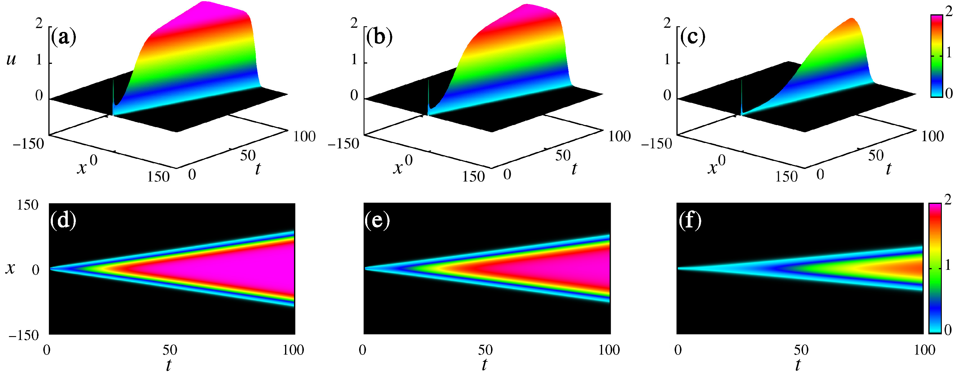
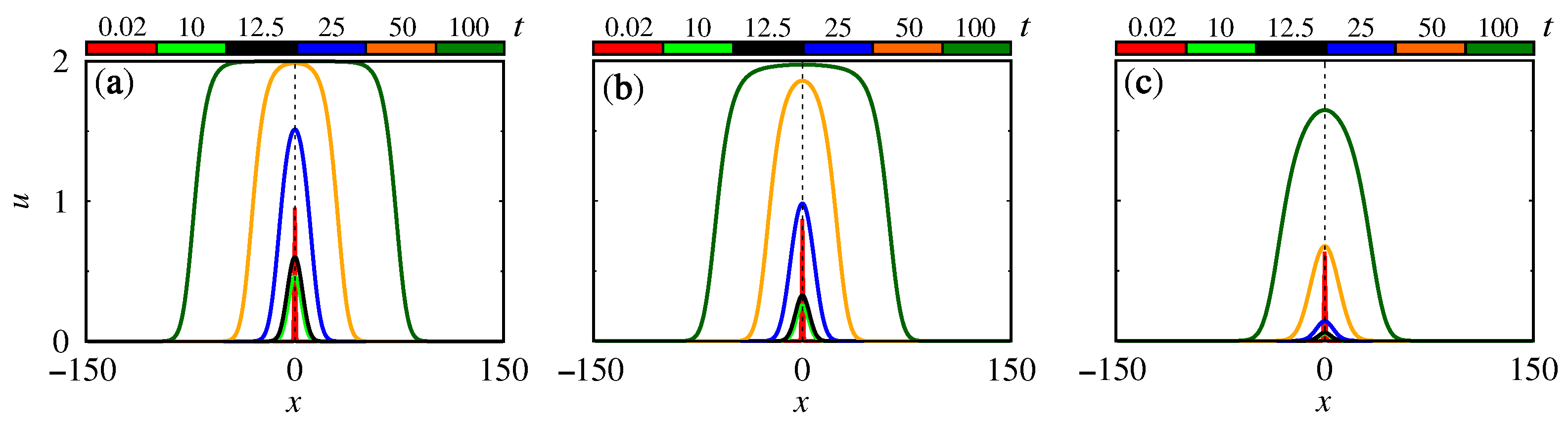
2.1. Time Fractional

Firstly, we start our investigation by considering the power law kernel (Equation (2)) only in the time operator. In this case, the dimensionless fractional Fisher equation is described as

$$\frac{{\partial }^{\alpha }}{\partial t^{\alpha }}u(x,t)=D\frac{{\partial }^2}{\partial x^2}u(x,t)+u(a-bu).$$

(7)

Due to the nature of the fractional operator and the nonlinearity in Equation (7), we restrict our analyses only to a numerical point of view. To obtain a complete discretization of Equation (7), we use the finite differences method [29,42]. The complete discussion about the method for the fractional reaction–diffusion equation under general kernels can be found in ref. [43]. To do that, we construct a grid defined by $[0,X]\times [0,T]$, where the space and time are discretized according to $x_i=i\mathrm{\Delta }x$ and $t_j=j\mathrm{\Delta }t$, respectively, where $i=0,1,\dots ,N_x$ and $j=0,1,\dots ,N_t$. The step sizes are defined by $\mathrm{\Delta }x=X/N_x$ and $\mathrm{\Delta }t=T/N_t$. In this work, we consider boundary conditions equal to $u(\pm X,t)=0$ and for numerical reasons, $X\to \infty$. The discrete form of Equation (7) is given by

$$u_{i,j+1}=u_{i,j}-\sum _{k=1}^j{\xi }_{k,\alpha }(u_{i,j+1-k}-u_{i,j-k})+D\Gamma (2-\alpha )\frac{\mathrm{\Delta }{t}^{\alpha }}{\mathrm{\Delta }{x}^2}(u_{i+1,j}-2u_{i,j}+u_{i-1,j})+\mathrm{\Delta }{t}^{\alpha }F(u_i,t_j),$$

(8)

where ${\xi }_{k,\alpha }=[{(k+1)}^{1-\alpha }-k^{1-\alpha }]$ and $F(u_i,t_j)=u_{i,j}(a-b{u}_{i,j})$. A detailed derivation of Equation (8) is shown in ref. [43]. It is worth mentioning that this choice for the spatial operator allows us to obtain an equivalent to the Riesz differential operator for the interval [43,44], i.e., $-\infty <x<\infty$, which, for practical proposes is considered finite $-X\le x\le X$ (with $\left|X\right|\to \infty$) to perform the numerical calculations. In this manner, the Caputo differential operator applied for the spatial variable behaves like the Riesz differential operator. Similar developments have been performed using the Riemann–Liouville operator in ref. [45]. We consider $u(x,0)=[\left(e^{-x^2/2{\sigma }^2}\right)/\left(2\pi {\sigma }^2\right)]$, $\sigma =0.4$, $\mathrm{\Delta }t=0.01$, $\mathrm{\Delta }x=0.6$, $D=1$, $a=0.2$ and $b=0.1$. In this work, we choose $a>b$ to obtain a non-null steady state. However, the values of the parameter are arbitrary.

Figure 1a–c displays the 3-dimensional solution with the respective density plots in Figure 1d–f. Figure 1a,d are for $\alpha =0.99$ (value near $\alpha =1$), while Figure 1b,e are for $\alpha =0.9$ (a considerable deviation of $\alpha =1$) and the Figure 1c,f are for $\alpha =0.7$ (a large deviation of $\alpha =1$). At the beginning of diffusion, the Gaussian packet spreads without the influence of reaction terms. However, after a certain time, the system starts to gain the shape of logistical growth, which is limited by K. This dynamic is sharper in Figure 1a,d, while in Figure 1b,e,c,f, the packets spread with low velocity, proportionally with $\alpha$ decrease. The decrease in the spread velocity implies a delay in reaching the steady solution.

The delayed process, shown in Figure 1, is more evident when we observe the profiles in Figure 2 for $t=0.02$ (red line), $t=10$ (green line), $t=12.5$ (black line), $t=25$ (blue line), $t=50$ (orange line) and $t=100$ (dark green line). Figure 2a–c we consider $\alpha =0.99$, $\alpha =0.9$ and $\alpha =0.7$, respectively. The amplitude of $u(x,t)$ depends on the value of $\alpha$. The solution for $\alpha =0.99$ reaches the steady state in approximately $t=52$, and for $\alpha =0.9$, spends $t\approx 95$. For $\alpha =0.7$, the time is superior to 100. Furthermore, we verify that the Gaussian package deforms over time.

As observed in 3-dimensional and profile representation, the packet follows a distribution without the influence of reaction terms and afterward obeys the logistic growth. To quantify the spread, we use the inverse of the square of the central peak, i.e., $u{(0,t)}^{-2}$ [37]. Considering the normalized function $u{(0,t)}^{-2}$, Figure 3 displays the distribution behavior of the Gaussian packet by the red points for $\alpha =0.99$ (Figure 3a), orange points for $\alpha =0.9$ (Figure 3b), and green points for $\alpha =0.7$ (Figure 3c). Discarding transient time ($t>0.04$), the displacement can be described by a power law function given by $\propto t^S$ until $t={10}^0$, where the S parameter is related to the anomalous relaxation process [37]. However, observing the distribution $u{(0,t)}^{-2}$, a nonlinear dynamics emerge. In this way, an adjustment given by a power law is not appropriate to capture this nonlinearity effect. In an attempt to capture these dynamics, we test q-exponential distributions [31]. In our simulations, the q-exponential that better fits the dynamics is the q-Weibull, which is given by

$$P_{qW}\left(t\right)=p_0\frac{r{t}^{r-1}}{t_0^r}{exp}_q\left[-{\left(\frac{t}{t_0}\right)}^r\right],$$

(9)

where the q-exponential is defined as follows:

$$\begin{array}{c}\hfill {exp}_q\left[x\right]=\left\{\begin{array}{cc}{[1+(1-q)x]}^{\frac{1}{1-q}}& ,x\ge 1/(q-1)\\ 0& ,x<1/(q-1)\end{array}\right..\end{array}$$

(10)

The q-Weibull adjustment depends on p₀, r, t₀ and q parameters. In the Figure 3a–c the black curve shows the adjustment given by Equation (9). To obtain the better parameters of Equation (9) that adjust the simulated points, we use the software Gnuplot 5.4.10 and we found the following parameters for each case: $p_0=4.96$, $r=1.75$, $t_0=4.07$ and $q=1.43$ for Figure 3a; $p_0=5.98$, $r=1.73$, $t_0=4.87$ and $q=1.35$ for Figure 3b; and $p_0=9.58$, $r=1.74$, $t_0=7.81$, and $q=1.31$ for Figure 3c. For the adjusted curve generated by these parameters, we compute the Pearson correlation coefficient (r), using the package SciPy in Python [46], and obtain, for Figure 3a, $r=0.9992$; for Figure 3b, $r=0.9997$; and for Figure 3c, $r=0.9996$. In addition, the respective mean square error is 0.012, 0.005 and 0.007. For these parameters, the respective absolute errors are displayed through blue points below the panel. Figure 3a, Equation (9) describes the points with great accuracy until $t\approx 52$, namely the time in which the distribution reaches a constant. On the other hand, as we decrease $\alpha$, the q-Weibull does not fit the points for $t<{10}^0$ with great accuracy. However, the distribution adjusts the simulated points for a long time, i.e., $t>50$. It is worth mentioning that q-Weibull is a type of stretched exponential in the sense of Tsallis distributions. In this way, the stretch is governed by the powers r and q. Our results suggest that as $\alpha$ decreases, the q parameter decreases, and the r seems to remain around $1.74$.

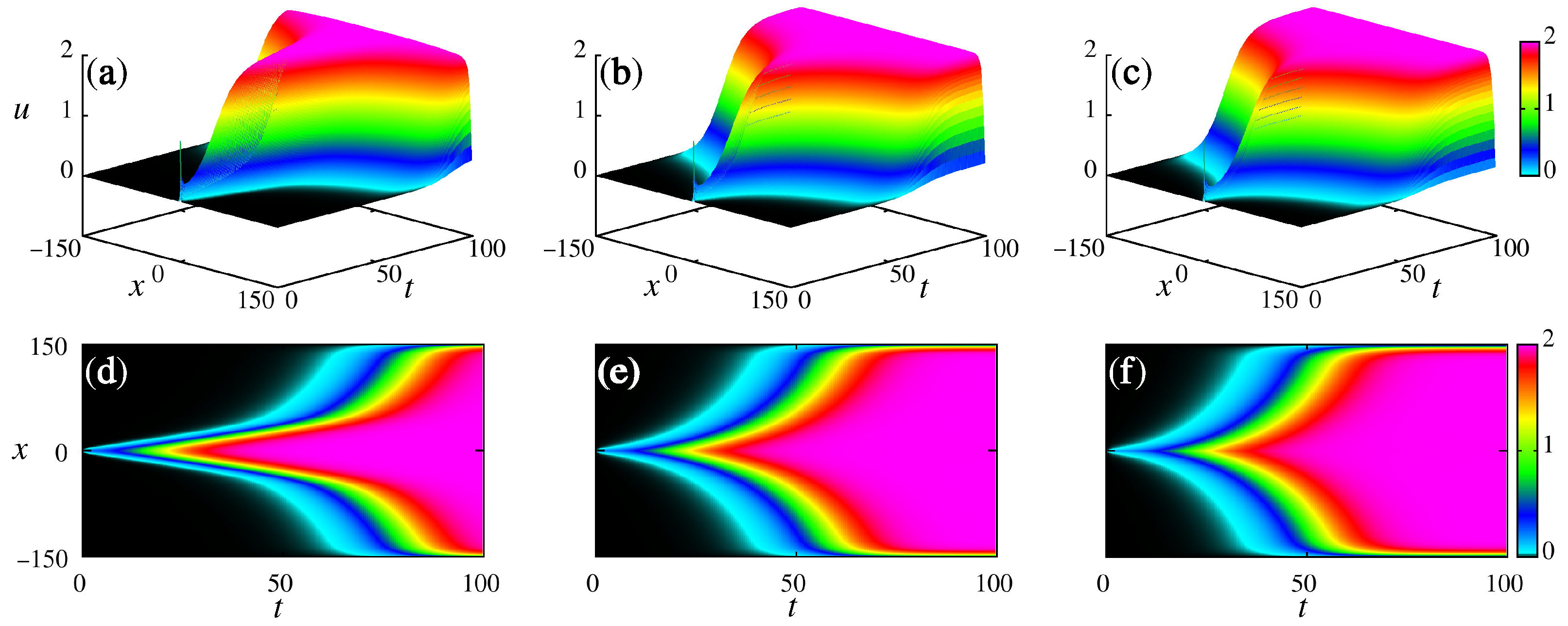
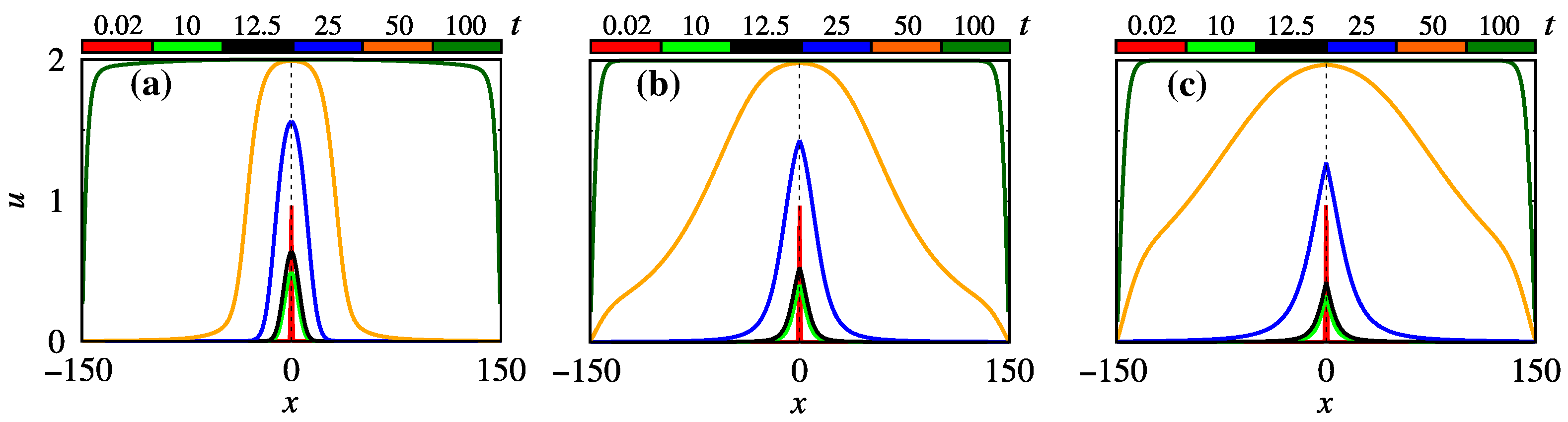
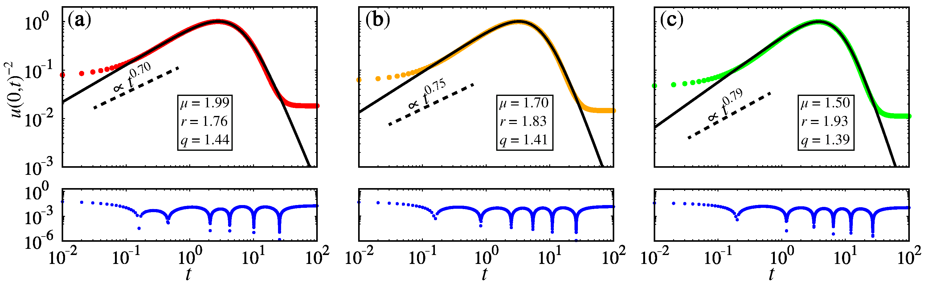
2.2. Space Fractional

To study the effects of a non-integer operator in a space derivative, we consider the usual operator in the time derivative and Caputo’s definition of the space operator. In this way, Equation (1) becomes

$$\frac{\partial }{\partial t}u(x,t)=D\frac{{\partial }^{\mu }}{\partial x^{\mu }}u(x,t)+u(a-bu),$$

(11)

with numerical schemes, equal to the one developed in ref. [43], given by

$$\begin{array}{ccc}\hfill u_{i,j+1}& =& u_{i,j}+\frac{D}{\Gamma (3-\mu )}\frac{\mathrm{\Delta }t}{\mathrm{\Delta }{x}^{\mu }}\sum _{n=0}^{i-1}{\xi }_{n,\mu }(u_{i-n+1,j}-2u_{i-n,j}+u_{i-n-1,j})+\mathrm{\Delta }tF(u_i,t_j),\hfill \end{array}$$

(12)

where ${\xi }_{n,\mu }=[{(n+1)}^{2-\mu }-n^{2-\mu }]$ and $F(u_i,t_j)=u_{i,j}(a-b{u}_{i,j})$. Note that the solutions of the fractional diffusion equations in the absence of reaction terms can be related to the Lévy distributions. The distributions that emerge from the Tsallis framework are essentially power laws and can also be connected with the Lévy distributions in the asymptotic limit for a suitable choice of the parameter q. These results allow us to connect these distributions in the asymptotic limit as performed in refs. [47,48].

A numerical solution for Equation (12) is exhibited in Figure 4, where we consider $u(x,0)=e^{-x^2/2{\sigma }^2}/\left(2\pi {\sigma }^2\right)$, $\sigma =0.4$, $\mathrm{\Delta }t=0.01$, $\mathrm{\Delta }x=0.6$, $D=1$, $a=0.2$ and $b=0.1$. Figure 4a,d are for $\mu =1.99$, Figure 4b,e for $\mu =1.7$, and Figure 4c,f for $\mu =1.5$. These choices of $\mu$ represent a small, medium, and large deviation from the standard value, i.e., $\mu =2$. The effects of space fractional derivatives contribute to the spread of the package. As $\mu$ decreases, the package occupies a larger space region.

Considering $\mu =1.99$, $\mu =1.7$ and $\mu =1.5$, Figure 5a–c shows the respective profiles, for $t=0.02$ (red line), $t=10$ (green line), $t=12.5$ (black line), $t=25$ (blue line), $t=50$ (orange line) and $t=100$ (dark green line). As observed in Figure 4, the effects of fractional space derivative widen the packet spread. For example, upon comparing the orange line ($t=50$) in the three panels, it is possible to note that the profile in Figure 5c is wider compared to cases in Figure 5a,b. This indicates that the smaller the $\mu$ value, the larger the package will open.

Considering the fractional operator acting only in the space derivative, we can also describe the behavior in the range $t\in (0.01,0.04)$ by a power law. For $\mu =1.99$, Figure 6a, the slope is 0.70. For $\mu =1.7$, Figure 6b, the slope is 0.75. Finally, for $\mu =1.5$, Figure 6c, the slope is 0.79. As $\mu$ decreases, the slope increases. These slopes are associated with an anomalous diffusion process. However, as in the case where we employ a time fractional derivative, the considered power law is not able to describe the whole transient. Once again, in an attempt to describe the whole transient, we adjust Equation (9) to the points obtained from the simulation. The red, orange and green lines correspond to $\mu =1.99$, $\mu =1.7$ and $\mu =1.5$, while the black line is the adjustment. The adjusted parameters for Figure 6a are $p_0=4.84$, $r=1.76$, $t_0=3.99$ and $q=1.44$; for Figure 6b are $p_0=5.29$, $r=1.83$, $t_0=4.47$ and $q=1.41$; and for Figure 6c are $p_0=5.71$, $r=1.93$, $t_0=5.00$ and $q=1.39$. For these parameters, we compute the absolute error among the simulated and adjusted points and display the results by the blue points below the panels. In this case, we observe that the absolute error oscillates in the range $({10}^{-6},{10}^{-3})$ for the time interval $t\in ({10}^{-1},3\times {10}^1)$. The maximum error, for the three cases, occurs when $t\in ({10}^{-2},{10}^{-1})$ and $t\in (5\times {10}^1,{10}^2)$. The correlation coefficient for the results in Figure 6a is $r=0.9991$, Figure 6b is $r=0.9994$ and Figure 6c is $r=0.9996$, with a mean square error equal to 0.013, 0.011 and 0.008, respectively. It is worth mentioning that in this approach, r depends on $\mu$. On the other hand, the q parameter decreases as a function of $\mu$. The other parameter related to the stretched exponential, i.e., r, increases as $\mu$ decreases.

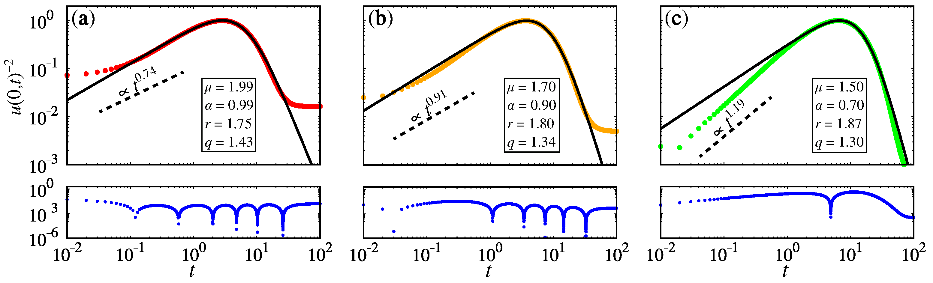
2.3. Time–Space Fractional

Considering both non-integer operators in Equation (1), the fractional Fisher equation becomes

$$\frac{{\partial }^{\alpha }}{\partial t^{\alpha }}u(x,t)=D\frac{{\partial }^{\mu }}{\partial x^{\mu }}u(x,t)+u(a-bu),$$

(13)

with a discrete form [43] equal to

$$\begin{array}{ccc}\hfill u_{i,j+1}& =& u_{i,j}-\sum _{k=1}^j{\xi }_{k,\alpha }(u_{i,j+1-k}-u_{i,j-k})+\hfill \\ & +& D\frac{\Gamma (2-\alpha )}{\Gamma (3-\mu )}\frac{\mathrm{\Delta }{t}^{\alpha }}{\mathrm{\Delta }{x}^{\mu }}\sum _{n=0}^{i-1}{\xi }_{n,\mu }(u_{i-n+1,j}-2u_{i-n,j}+u_{i-n-1,j})\hfill \\ & +& \mathrm{\Delta }{t}^{\alpha }\Gamma (2-\alpha )F(u_i,t_j),\hfill \end{array}$$

(14)

where ${\xi }_{k,\alpha }=[{(k+1)}^{1-\alpha }-k^{1-\alpha }]$, ${\xi }_{n,\mu }=[{(n+1)}^{2-\mu }-n^{2-\mu }]$ and $F(u_i,t_j)=u_{i,j}(a-b{u}_{i,j})$.

Considering $u(x,0)=[\left(e^{-x^2/2{\sigma }^2}\right)/\left(2\pi {\sigma }^2\right)]$, $\sigma =0.4$, $\mathrm{\Delta }t=0.01$, $\mathrm{\Delta }x=0.6$, $D=1$, $a=0.2$ and $b=0.1$, Figure 7 shows the numerical solutions for Equation (14). Figure 7a–c exhibit the 3-dimensional solution, while Figure 7d–f display the density plots. We consider $\alpha =0.99$ and $\mu =1.99$ in Figure 7a,d; $\alpha =0.9$ and $\mu =1.7$ in Figure 7b,e; and $\alpha =0.7$ and $\mu =1.5$ in Figure 7c,f. The package, initially Gaussian, suffers the influence of both non-integer derivatives. Nonetheless, the diffusion accentuates the effects of the time operator more than the space one. Another observation is that the time to reach the steady state is practically the same, as shown in Figure 1.

The profiles for $t=0.02$ (red line), $t=10$ (green line), $t=12.5$ (black line), $t=25$ (blue line), $t=50$ (orange line) and $t=100$ (dark green line) are displayed in Figure 8a for $\alpha =0.99$ and $\mu =1.99$; Figure 8b for $\alpha =0.9$ and $\mu =1.7$; and Figure 8c for $\alpha =0.7$ and $\mu =1.5$. The profiles show that the spread is similar when it is only governed by the time fractional operators. This difference occurs due to the multiplicative factors in Equation (14).

The transient dynamics can also be described by Equation (9) when we combine both fractional operators in time and space. Figure 9 displays the simulated points in (a) red, (b) orange, and (c) green and the adjusted curve in the black lines, for $\mu =1.99$ and $\alpha =0.99$, $\mu =1.70$ and $\alpha =0.90$, and $\mu =1.50$ and $\alpha =0.70$, respectively. The result in blue points shows the absolute error among the simulated points and the ones obtained by the adjustment using Equation (9). The adjustment parameters are $p_0=4.97$, $r=1.75$, $t_0=4.09$ and $q=1.43$ for Figure 9a; $p_0=6.42$, $r=1.80$, $t_0=5.35$ and $q=1.34$ for Figure 9b; and $p_0=11$, $r=1.87$, $t_0=9.35$ and $q=1.30$ for Figure 9c. By computing the correlation, we obtain (a) $r=0.9992$, (b) $r=0.9997$ and (c) $r=0.9996$. Furthermore, the mean square error is 0.012, 0.005 and 0.007 in Figure 9a–c, respectively. Due to the influence of both operators, the packet is well described by Equation (9) in the region $t\in ({10}^0,\tau )$, where $\tau =52.2$ in Figure 9a, $\tau \approx 95$ in Figure 9b and $\tau >100$ in Figure 9c. These results are similar to those shown in Figure 3. Furthermore, the r value is close to the value obtained when only the time fractional operator is considered. On the other hand, the value of q is the same. These results confirm the fact that the time fractional operator causes more influence in the system than the space operator.

3. Conclusions

In this work, we have conducted a study of the numerical solutions of the fractional Fisher’s equation. As a fractional operator, we employed the Caputo definition discretized by the finite difference scheme. Considering a Gaussian package as an initial condition, we investigated three scenarios in terms of fractional operators. We consider time and space operators in the first and second scenarios. The last one considered time and space operators in the reaction–diffusion equation. Due to the logistic terms in the reaction–diffusion equation, the system evolved until it reached its stability solutions, which are completely determined by logistics terms.

Our results show that the transient dynamics are not well described by power law functions, such as in some cases of the diffusion processes. From our simulations, the function that best fits the transient is a generalized q-exponential, from a Tsallis framework. In our simulations, we have different behaviors exhibited by the solution. One for a small time, where the influence of the reaction terms is not pronounced. Another is exhibited for a long time, when the reaction terms have a pronounced effect and an intermediate behavior connecting these two limits. On the other hand, the Tsallis framework provides functions with a large class of behaviors that can also be connected with the solutions of the nonlinear equations, such as the porous media equation, establishing a connection between the parameters for the distributions. In this sense, we use the functions that emerge from the Tsallis framework to capture the behavior exhibited by the spreading of the system in a range of time, suggesting that the system’s relaxation process is anomalous and may be investigated by a generalized context. This is a relevant and new finding for the q-distributions. Furthermore, it is important to mention that the adjustment parameters from q-exponential depend on the fractional order. This is expected once the transient strongly depends on the time order derivative. In addition, we observed that the fractional operator in space does not significantly influence the transient. In terms of fractional calculus, our results contribute to a better understanding of Fisher’s equation in a generalized way. These achievements can be used to comprehend better phenomena described by Fisher’s equation, such as epidemics and bacteria growth [6] and chemical kinetics [4]. In future works, we plan to employ the methodology described in this research in real applications, such as in the field of biochemistry [5].

References

1. Zhou, Q.; Ekici, M.; Sonmezoglu, A.; Manafian, J.; Khaleghizadeh, S.; Mirzazadeh, M. Exact solitary wave solutions to the generalized Fisher equation. Optik 2016, 127, 12085–12092. [Google Scholar] [CrossRef]
2. El-Hachem, M.; McCue, S.W.; Jin, W.; Du, Y.; Simpson, M.J. Revisiting the Fisher–Kolmogorov–Petrovsky–Piskunov equation to interpret the spreading–extinction dichotomy. Proc. R. Soc. A 2019, 475, 20190378. [Google Scholar] [CrossRef] [PubMed]
3. Chandraker, V.; Awasthi, A.; Jayaraj, S. A Numerical Treatment of Fisher Equation. Procedia Eng. 2015, 127, 1256–1262. [Google Scholar] [CrossRef]
4. Ross, J.; Villaverde, A.F.; Banga, J.R.; Vázquez, S.; Morán, F. A generalized Fisher equation and its utility in chemical kinetics. Proc. Natl. Acad. Sci. USA 2010, 107, 12777–12781. [Google Scholar] [CrossRef] [PubMed]
5. Nardini, J.T.; Bortz, D.M. Investigation of a structured Fisher’s equation with applications in biochemistry. SIAM J. Appl. Math. 2018, 78, 1712–1736. [Google Scholar] [CrossRef] [PubMed]
6. Kenkre, V. Results from variants of the Fisher equation in the study of epidemics and bacteria. Phys. A Stat. Mech. Appl. 2004, 342, 242–248. [Google Scholar] [CrossRef]
7. Wen-Shan, D.; Hong-Juan, Y.; Yu-Ren, S. An exact solution of Fisher equation and its stability. Chin. Phys. 2006, 15, 1414. [Google Scholar] [CrossRef]
8. Gazdag, J.; Canosa, J. Numerical solution of Fisher’s equation. J. Appl. Probab. 1974, 11, 445–457. [Google Scholar] [CrossRef]
9. Tompson, A.; Dougherty, D. Particle-grid methods for reacting flows in porous media with application to Fisher’s equation. Appl. Math. Model. 1992, 16, 374–383. [Google Scholar] [CrossRef]
10. Mavoungou, T.; Cherruault, Y. Numerical study of fisher’s equation by Adomian’s method. Math. Comput. Model. 1994, 19, 89–95. [Google Scholar] [CrossRef]
11. Hariharan, G.; Kannan, K.; Sharma, K. Haar wavelet method for solving Fisher’s equation. Appl. Math. Comput. 2009, 211, 284–292. [Google Scholar] [CrossRef]
12. Kırlı, E.; Irk, D. Efficient techniques for numerical solutions of Fisher’s equation using B-spline finite element methods. Comput. Appl. Math. 2023, 42, 151. [Google Scholar] [CrossRef]
13. Roessler, J.; Hüssner, H. Numerical solution of the 1 + 2 dimensional Fisher’s equation by finite elements and the Galerkin method. Math. Comput. Model. 1997, 25, 57–67. [Google Scholar] [CrossRef]
14. Loyinmi, A.; Akinfe, K. Exact solutions to the family of Fisher’s reaction-diffusion equation using Elzaki homotopy transformation perturbation method. Eng. Rep. 2020, 2, e12084. [Google Scholar] [CrossRef]
15. Li, W.; Pang, Y. Application of Adomian decomposition method to nonlinear systems. Adv. Differ. Equ. 2020, 2020, 1–17. [Google Scholar] [CrossRef]
16. Hariharan, G.; Kannan, K. Haar wavelet method for solving some nonlinear parabolic equations. J. Math. Chem. 2010, 48, 1044–1061. [Google Scholar] [CrossRef]
17. Evangelista, L.R.; Lenzi, E.K. An Introduction to Anomalous Diffusion and Relaxation; Springer Nature: Berlin/Heidelberg, Germany, 2023. [Google Scholar]
18. Herrmann, R. Fractional Calculus: An Introduction for Physicists; World Scientific: Singapore, 2014. [Google Scholar]
19. Guo, B.; Pu, X.; Huang, F. Fractional Partial Differential Equations and Their Numerical Solutions; World Scientific: Singapore, 2015. [Google Scholar]
20. Rosseto, M.; Evangelista, L.; Lenzi, E.; Zola, R.; Ribeiro de Almeida, R. Frequency-Dependent Dielectric Permittivity in Poisson–Nernst–Planck Model. J. Phys. Chem. B 2022, 126, 6446–6453. [Google Scholar] [CrossRef]
21. Ahmed, H.F. Efficient methods for the analytical solution of the fractional generalized Fisher equation. J. Fract. Calc. Appl. 2019, 10, 85–104. [Google Scholar]
22. Hashemi, M.; Baleanu, D. On the Time Fractional Generalized Fisher Equation: Group Similarities and Analytical Solutions. Commun. Theor. Phys. 2016, 65, 11. [Google Scholar] [CrossRef]
23. Mirzazadeh, M. A novel approach for solving fractional Fisher equation using differential transform method. Pramana J. Phys. 2016, 86, 957–963. [Google Scholar] [CrossRef]
24. Bayrak, M.A.; Demir, A.; Ozbilge, E. On the numerical solution of conformable fractional diffusion problem with small delay. Numer. Methods Partial. Differ. Equ. 2020, 2022, 177–189. [Google Scholar] [CrossRef]
25. Majeed, A.; Kamran, M.; Abbas, M.; Singh, J. An Efficient Numerical Technique for Solving Time-Fractional Generalized Fisher’s Equation. Front. Phys. 2020, 8, 1–11. [Google Scholar] [CrossRef]
26. Majeed, A.; Kamran, M.; Iqbal, M.K.; Baleanu, D. Solving time fractional Burgers’ and Fisher’s equations using cubic B-spline approximation method. Adv. Differ. Equ. 2020, 2020, 1–15. [Google Scholar] [CrossRef]
27. Rashid, S.; Hammouch, Z.; Aydi, H.; Ahmad, A.G.; Alsharif, A.M. Novel Computations of the Time-Fractional Fisher’s Model via Generalized Fractional Integral Operators by Means of the Elzaki Transform. Fractal Fract. 2021, 5, 94. [Google Scholar] [CrossRef]
28. Veeresha, P.; Prakasha, D.G.; Baskonus, H.M. Novel simulations to the time-fractional Fisher’s equation. Math. Sci. 2019, 13, 33–42. [Google Scholar] [CrossRef]
29. Crank, J. The Mathematics of Diffusion; Oxford University Press: Oxford, UK, 1975. [Google Scholar]
30. Picoli, S., Jr.; Mendes, R.S.; Malacarne, L.C.; Lenzi, E.K. Scaling behavior in the dynamics of citations to scientific journals. Europhys. Lett. 2006, 75, 673. [Google Scholar] [CrossRef]
31. Picoli, S., Jr.; Mendes, R.S.; Malacarne, L.C.; Santos, R.P.B. q-Distributions in complex systems: A brief review. Braz. J. Phys. 2009, 39, 468–474. [Google Scholar] [CrossRef]
32. Tsallis, C. Possible generalization of Boltzmann-Gibbs statistics. J. Stat. Phys. 1988, 52, 479–487. [Google Scholar] [CrossRef]
33. Sigalotti, L.D.G.; Ramírez-Rojas, A.; Vargas, C. Tsallis q-Statistics in Seismology. Entropy 2023, 25, 408. [Google Scholar] [CrossRef] [PubMed]
34. Murray, J.D. Mathematical Biology: I: An Introduction; Springer: Berlin/Heidelberg, Germany, 2002. [Google Scholar]
35. Murray, J.D. Mathematical Biology: II: Spatial Models and Biomedical Applications; Springer: Berlin/Heidelberg, Germany, 2003. [Google Scholar]
36. Rahimy, M. Applications of fractional differential equations. Appl. Math. Sci. 2010, 4, 2453–2461. [Google Scholar]
37. Evangelista, L.R.; Lenzi, E.K. Fractional Diffusion Equations and Anomalous Diffusion; Cambridge University Press: Cambridge, UK, 2018. [Google Scholar]
38. Lenzi, E.; Lenzi, M.; Ribeiro, H.; Evangelista, L. Extensions and solutions for nonlinear diffusion equations and random walks. Proc. R. Soc. A 2019, 475, 20190432. [Google Scholar] [CrossRef]
39. Mendez, V.; Fedotov, S.; Horsthemke, W. Reaction-Transport Systems: Mesoscopic Foundations, Fronts, and Spatial Instabilities; Springer Science & Business Media: Berlin/Heidelberg, Germany, 2010. [Google Scholar]
40. Henry, B.I.; Wearne, S.L. Fractional reaction–diffusion. Phys. Stat. Mech. Appl. 2000, 276, 448–455. [Google Scholar] [CrossRef]
41. Henry, B.; Langlands, T.; Wearne, S. Anomalous diffusion with linear reaction dynamics: From continuous time random walks to fractional reaction-diffusion equations. Phys. Rev. E 2006, 74, 031116. [Google Scholar] [CrossRef] [PubMed]
42. Guo, X.; Xu, M. Some physical applications of fractional Schrödinger equation. J. Math. Phys. 2006, 47, 082104. [Google Scholar] [CrossRef]
43. Gabrick, E.C.; Protachevicz, P.R.; Lenzi, E.K.; Sayari, E.; Trobia, J.; Lenzi, M.K.; Borges, F.S.; Caldas, I.L.; Batista, A.M. Fractional Diffusion Equation under Singular and Non-Singular Kernel and Its Stability. Fractal Fract. 2023, 7, 792. [Google Scholar] [CrossRef]
44. Blaszczyk, T.; Bekus, K.; Szajek, K.; Sumelka, W. On numerical approximation of the Riesz–Caputo operator with the fixed/short memory length. J. King Saud Univ. Sci. 2021, 33, 101220. [Google Scholar] [CrossRef]
45. Yang, Q.; Liu, F.; Turner, I. Numerical methods for fractional partial differential equations with Riesz space fractional derivatives. Appl. Math. Model. 2010, 34, 200–218. [Google Scholar] [CrossRef]
46. Virtanen, P.; Gommers, R.; Oliphant, T.E.; Haberland, M.; Reddy, T.; Cournapeau, D.; Burovski, E.; Peterson, P.; Weckesser, W.; Bright, J.; et al. SciPy 1.0: Fundamental Algorithms for Scientific Computing in Python. Nat. Methods 2020, 17, 261–272. [Google Scholar] [CrossRef]
47. Bologna, M.; Tsallis, C.; Grigolini, P. Anomalous diffusion associated with nonlinear fractional derivative Fokker-Planck-like equation: Exact time-dependent solutions. Phys. Rev. E 2000, 62, 2213. [Google Scholar] [CrossRef]
48. Tsallis, C.; Lenzi, E. Anomalous diffusion: Nonlinear fractional Fokker–Planck equation. Chem. Phys. 2002, 284, 341–347. [Google Scholar] [CrossRef]
Figure 1. Gaussian package diffusion in the (ac), followed by its density plot in the (df), respectively. We consider α = 0.99 in (a,d), α = 0.90 in (b,e), and α = 0.7 in (c,f).
Fractalfract 08 00143 g001
Figure 2. Profiles of Gaussian package spread for (a) α = 0.99 , (b) α = 0.9 and (c) α = 0.7 .
Fractalfract 08 00143 g002
Figure 3. Displacements ( u ( 0 , t ) 2 ) of Gaussian package for α = 0.99 in the red line (a), α = 0.9 in the orange line (b) and α = 0.7 in the green line (c). The black lines indicated the adjusment given by Equation (9) for each case. (a) adjustment parameters are given by p 0 = 4.96 , r = 1.75 , t 0 = 4.07 and q = 1.43 . (b), the parameters are p 0 = 5.98 , r = 1.73 , t 0 = 4.87 and q = 1.35 . The parameters are p 0 = 9.58 , r = 1.74 , t 0 = 7.81 and q = 1.31 in (c). The blue points in the below panels represent the respective absolute error among simulated and theoretical points.
Fractalfract 08 00143 g003
Figure 4. Diffusion of a Gaussian package in (ac). Density plot of Gaussian package in (df). (a,d) are for μ = 1.99 , while (b,e) are for μ = 1.7 . In (c,f), we consider μ = 1.5 .
Fractalfract 08 00143 g004
Figure 5. Profiles of Gaussian package for (a) μ = 1.99 , (b) μ = 1.7 and (c) μ = 1.5 .
Fractalfract 08 00143 g005
Figure 6. Displacements ( u ( 0 , t ) 2 ) of the Gaussian package for μ = 1.99 in the red line (a), μ = 1.7 in the orange line (b), and μ = 1.5 in the green line (c). The black line is the adjusted curve with parameters equal to: (a) p 0 = 4.84 , r = 1.76 , t 0 = 3.99 and q = 1.44 ; (b) p 0 = 5.29 , r = 1.83 , t 0 = 4.47 and q = 1.41 ; (c) p 0 = 5.71 , r = 1.93 , t 0 = 5.00 and q = 1.39 . The blue points in the below panels show the absolute error computed considering the black and simulated points.
Fractalfract 08 00143 g006
Figure 7. Diffusion of a Gaussian package in (ac). Density plot of Gaussian package in (df). In (a,d), we consider μ = 1.99 and α = 0.99 ; in (b,c), we use μ = 1.7 and α = 0.9 ; and in (c,f), we consider μ = 1.5 and α = 0.7 .
Fractalfract 08 00143 g007
Figure 8. Profiles of Gaussian package for (a) μ = 1.99 and α = 0.99 , (b) μ = 1.7 and α = 0.9 , and (c) μ = 1.5 and α = 0.7 .
Fractalfract 08 00143 g008
Figure 9. Displacements ( u ( 0 , t ) 2 ) of Gaussian package for (a) α = 0.99 and μ = 1.99 in the red line, (b) μ = 1.7 and α = 0.9 in the orange line and (c) μ = 1.5 and α = 0.7 in the green line. The black curve is the adjusted curve with parameters equal to p 0 = 4.97 , r = 1.75 , t 0 = 4.09 and q = 1.43 , for (a); p 0 = 6.42 , r = 1.80 , t 0 = 5.35 and q = 1.34 , for (b); p 0 = 11 , r = 1.87 , t 0 = 9.35 and q = 1.30 , for (c). The blue points in the below panels show the absolute error computed considering the black and simulated points.
Fractalfract 08 00143 g009
Disclaimer/Publisher’s Note: The statements, opinions and data contained in all publications are solely those of the individual author(s) and contributor(s) and not of MDPI and/or the editor(s). MDPI and/or the editor(s) disclaim responsibility for any injury to people or property resulting from any ideas, methods, instructions or products referred to in the content.