Chaos, Fractionality, Nonlinear Contagion, and Causality Dynamics of the Metaverse, Energy Consumption, and Environmental Pollution: Markov-Switching Generalized Autoregressive Conditional Heteroskedasticity Copula and Causality Methods

Abstract

Metaverse (MV) technology introduces new tools for users each day. MV companies have a significant share in the total stock markets today, and their size is increasing. However, MV technologies are questioned as to whether they contribute to environmental pollution with their increasing energy consumption (EC). This study explores complex nonlinear contagion with tail dependence and causality between MV stocks, EC, and environmental pollution proxied with carbon dioxide emissions (CO₂) with a decade-long daily dataset covering 18 May 2012–16 March 2023. The Mandelbrot–Wallis and Lo’s rescaled range (R/S) tests confirm long-term dependence and fractionality, and the largest Lyapunov exponents, Shannon and Havrda, Charvât, and Tsallis (HCT) entropy tests followed by the Kolmogorov–Sinai (KS) complexity measure confirm chaos, entropy, and complexity. The Brock, Dechert, and Scheinkman (BDS) test of independence test confirms nonlinearity, and White‘s test of heteroskedasticity of nonlinear forms and Engle’s autoregressive conditional heteroskedasticity test confirm heteroskedasticity, in addition to fractionality and chaos. In modeling, the marginal distributions are modeled with Markov-Switching Generalized Autoregressive Conditional Heteroskedasticity Copula (MS-GARCH–Copula) processes with two regimes for low and high volatility and asymmetric tail dependence between MV, EC, and CO₂ in all regimes. The findings indicate relatively higher contagion with larger copula parameters in high-volatility regimes. Nonlinear causality is modeled under regime-switching heteroskedasticity, and the results indicate unidirectional causality from MV to EC, from MV to CO_2, and from EC to CO₂, in addition to bidirectional causality among MV and EC, which amplifies the effects on air pollution. The findings of this paper offer vital insights into the MV, EC, and CO₂ nexus under chaos, fractionality, and nonlinearity. Important policy recommendations are generated.

1. Introduction

Natural environmental systems can exhibit chaotic behavior due to the complexity of interactions between various factors [1]. Human activities, including those related to the development of digital technologies, can introduce disturbances that affect the balance of these systems. Still, this topic has found very limited applications in recent environmental studies. Several studies are currently exploring the potentially chaotic nature of environmental pollution. In 1963, Lorenz introduced a valuable tool to depict the dynamic characteristics of such systems [2]. The atmospheric system exhibits a complex and nonlinear structure, encompassing both stochastic and deterministic elements. Chaotic structures in the average ozone concentration within the atmospheric system are empirically shown in the literature [3,4]. Further, [5] demonstrated nonlinearity in NO₂ and CO using the Volterra–Wiener–Korenberg (VWK) method. Meanwhile, [6] uncovered evidence of chaotic structures in NO, CO, SO₂, PM10, and NO₂ with the utilization of the Lyapunov exponent. In addition, [7] detected chaotic characteristics in the air pollution index (API) in Lanzhou, northwest China; [8] explored chaotic dynamics of air pollution in India, China, and Türkiye; and [9] examined chaotic dynamics of air temperature with Lie group algebra. While these studies explored the factors affecting environmental pollution and the effects of metaverse and energy consumption, their chaotic structure with long-term dependence leading to nonlinearity in contagion and causal relations have not been explored in the literature.

The metaverse (MV) has an important potential to transform our daily lives in the near future, and MV technologies will also bring new business opportunities. In fact, by connecting virtual and physical spaces with virtual reality (VR), augmented reality (AR), and internet technologies (IT), the MV is expected to host a growing number of activities of people, which include working, shopping, attending schools, games, and entertainment. According to a survey conducted by Gartner, a leading information technology research and consultancy company, it is projected that by 2026, 25% of the global population will spend at least one hour per day in the MV, engaging in activities such as work, shopping, education, socializing, and entertainment [10].

Digital technologies, especially the MV, could have significant impacts on the chaotic nature of environmental pollution. It is very important to study the chaotic nature of both digital technology and environmental pollution under the influences of human behavior and new digital technologies. The chaotic structure relationship between energy prices, the metaverse, and environmental pollution is not inherently direct, but one can explore potential connections and interactions among these concepts. It is important to note that the metaverse is a concept that primarily refers to a virtual shared space created by the convergence of physical and virtual reality, including the sum of all virtual worlds, augmented reality, and the internet. The infrastructure required for the metaverse, including data centers, can contribute to environmental concerns if not managed sustainably. Energy consumption and electronic waste are potential issues. The development and maintenance of the infrastructure supporting the metaverse, such as servers and data centers, can contribute to pollution.

The massive energy requirement of MV technology and its significant environmental implications have been long foregone [11]. A projection from Global Bank Citi shows an even more serious situation: the number of MV users could reach up to 5 billion by 2030, and the MV economy could grow to a value of USD 8 to USD 13 trillion [12].

Establishing the MV requires both physical infrastructure and a reliable supply of electricity. Essential components of the infrastructure include hardware devices like VR headsets, which are crucial for delivering immersive virtual experiences to users. Moreover, upgrades to communication networks and data centers are necessary to enhance bandwidth, computing power, and speed, enabling the accommodation of a larger number of users and meeting their increased online activity requirements [13].

The impacts of the MV on energy consumption (EC) and environmental pollution have raised many concerns. As the MV expands and becomes more integrated into our daily lives, it will have various effects on energy and the environment. Regarding the energy problem, the operations of the MV necessitate a significant amount of energy required for servers, data centers, and devices such as the 3D, VR, and AR equipment involved in creating and maintaining the virtual environment [14]. Since no data exist specifically for the MV’s energy consumption in financial transactions, Bitcoin could be used instead for such analysis. It was shown that the mining of a single Bitcoin in 2021 led to the level of electricity consumption of a typical household over 12 years [15]. The yearly Bitcoin mining in the world sums to 200 TWh terawatt-hours, equivalent to the energy consumption of Thailand in a year [16]. For 2019, the energy consumption of Bitcoin mining was estimated to be significantly higher than the total energy consumption of Austria [17]. Further, Ref. [18] proposes a method to calculate the energy consumption of cryptocurrencies, and Digiconomist estimates Bitcoin’s peak yearly consumption as 204 TWh, which is expected to result in 95 million tons of CO₂ emissions per year [19]. At the same time, artificial intelligence (AI) technology has the potential to generate and populate virtual environments within the MV, leading to an extensive amount of energy demand. Some examples have been given for recent popular AI systems such as the OpenAI’s DALL-E. In those cases, these technologies are shown to require substantial computational power for both training the models and operating the environment. As a result, their environmental effects should be seriously considered. A recent study points out the inefficiency of the electricity grid and distribution for the proposed MV; however, the MV could also have a positive effect in the future if the technology is used to increase distributional efficiency with an effective matching of energy supply and demand [20].

Though this is the case, the investigation of the MV, energy consumption, and carbon dioxide (CO₂) emissions nexus is of vital importance to be measured empirically. To address these environmental concerns, it is crucial to implement sustainable practices and policies within the MV ecosystem. The high energy demand of the MV leads to increased greenhouse gas (GHG) emissions [14], which includes CO₂ emissions, a major contributor to the sera effect. The interconnectedness of the MV and the activities conducted are criticized for creating a significant carbon footprint [11]. Carbon footprint encompasses the emissions associated with the infrastructure, data storage, data transmission, and user activities [14]. In addition to the environmental effects of EC, further effects can be attributed to electronic waste generation (e-waste) and carbon the footprint associated with MV technologies and activities.

Although the impact of the metaverse on high energy demand and environmental pollution is emphasized by the above studies, these studies did not analyze chaotic structure. Existing explanations for analyzing the chaotic nature of environmental pollution remain incomplete without a comprehensive investigation of chaotic structures using the largest Lyapunov (λ) and Shannon entropy tests and without examining the long-term dependence and fractionality in environmental pollution. As we emphasized above, the chaotic structure is an important phenomenon of these series, and the analyzed variables have complex associations that could be altered even after a small shock is applied to their dynamics, leading to changes in their structures. To our knowledge, no empirical analyses exist for the assessment of contagion, tail dependence and causality dynamics, or possibly chaotic and fractional dynamics coupled with nonlinear relations between the MV, EC, and CO₂.

With a dataset that consists of daily observations for CO₂ emissions, energy consumption by the major cryptocurrency, and the MV stock index for a period covering 18 May 2012–16 March 2023, this study explores chaotic structure by using Lyapunov exponent tests [21] and Shannon entropy [22], long-term dependence and fractionality with rescaled range (R/S) and Lo’s modified R/S [23] tests, Geweke and Porter-Hudak’s and Robinson and Henry’s tests [24,25] for long memory, and estimation of fractional parameters. Afterward, the series and the relations among these series are modeled with nonlinear models and nonlinear causality tests aiming at capturing contagion, tail dependence, and causality.

Evidence of chaos is investigated by using the largest Lyapunov exponent (λ) and Shannon entropy [21,22]. λ is used to determine the sensitivity to primal conditions and identify the presence of chaotic motion. Hence, the detection of chaos in our study is conducted following a set of studies with this respect [21,26,27,28,29,30,31]. Further, the series is analyzed with the HCT entropy measure first developed by Havrda and Charvât [32] and afterward by Tsallis [33]. In addition, the series is analyzed with the Kolmogorov–Sinai (KS) complexity measure to examine different aspects of the dynamics for their dependence on initial conditions, chaos, complexity, and unpredictability [34]. In the second stage, long-term dependence is tested with the Malderbrot and Wallis R/S test [35] and Lo’s modified R/S test [23]. Long-memory and fractional parameters are further tested and estimated with Geweke and Porter-Hudak’s [24] and Robinson and Henry’s methods [25]. The series are examined for nonlinearity with the BDS test introduced by [36,37]. Heteroskedasticity is tested with two methods. The first is White’s Lagrange multiplier (LM) test [38], which is a robust test used to examine the existence of nonlinear forms of heteroskedasticity. The second is Engle’s ARCH-LM test, which follows the LM testing procedure to examine the non-existence of autoregressive conditional heteroskedasticity (ARCH) processes [39].

If the methods at the previous stages point at a chaotic structure, complexity, nonlinearity and fractionality, we use the Markov-Switching Generalized Autoregressive Conditional Heteroskedasticity Copula Causality (MS-GARCH–Copula Causality) method, a novel hybrid method benefiting from Markov-Switching GARCH models in marginal distributions, copula modeling for joint distributions for regime-dependent tail dependence and contagion, and regime-dependent causal inference as an extension of Kim’s GARCH–Copula Causality to regime-dependent nonlinear causality tests [40]. The approach has found recent applications for a nonlinear inquiry of regime-dependent contagion, tail dependence, and causality dynamics [41,42]. As it will be discussed, the MS-GARCH–Copula Causality method allows for the determination of ARCH and GARCH effects in different regimes in addition to persistence, contagion, and Granger causality in the presence of highly complex dynamics.

This manuscript consists of five sections. Section 1 covers the introduction and literature. Section 2 focuses on the methodology, Section 3 provides the dataset and empirical results, and Section 4 includes the conclusion and policy implications.

2. Methodology

This study uses the Markov-Switching (MS) Autoregressive Moving Average (ARMA) Generalized Autoregressive Conditional Heteroskedasticity (GARCH) Copula Causality, hence forth, the MS-GARCH–Copula Causality method [40]. This new method generalizes Kim’s [43] causality tests to copula and GARCH with Markov regime switching. A time series r_t is assumed to follow a nonlinear conditional mean, as in Equation (1), and nonlinear conditional variance, as in Equation (2) [44,45],

$$r_t={\theta }_{0,\left(st\right)}+{\sum }_{i=1}^f{\theta }_{i,\left(st\right)}{r}_{t-i,\left(st\right)}+{\sum }_{n=1}^m{\lambda }_{n,\left(st\right)}{\epsilon }_{t-n,\left(st\right)}+{\epsilon }_{t,\left(st\right)}$$

(1)

$${\sigma }_{t,\left(st\right)}^2={\alpha }_{0,\left(st\right)}+{\sum }_{n=1}^q{\alpha }_{i,\left(st\right)}{\sigma }_{t-n,\left(st\right)}+{\sum }_{n=1}^p{\beta }_{i,\left(st\right)}{\epsilon }_{t-n,\left(st\right)}^2$$

(2)

where

$${\sigma }_{t-i-1,(st-i)}=E\left({\epsilon }_{t-i-1,(st-i-1)}|s_{t-i},r_{t-i-1}\right)$$

(3)

In Equation (2), non-negativity constrained parameters $\varphi ,\alpha ,\kappa ,\beta >0$ allow for strictly positive variance processes similar to the single-regime GARCH model of [46]. Switching between distinct regimes is governed with a process of Markov-switching as

$${\pi }_{nt}=\mathrm{Pr}\left[s_t=j\left|r_{t-1}\right.\right]={\displaystyle {\sum }_{i=0}^1\mathrm{Pr}\left[s_t=j\left|s_{t-1}=i\right.\right]}\mathrm{Pr}\left[s_t=j\left|r_{t-1}\right.\right]{\displaystyle {\sum }_{i=0}^1{\psi }_{ni}}{\pi }_{it-1}^{*}$$

(4)

with

$$L={\prod }_{t=1}^{T}f\left(r_t|s_{t=i},r_{t-1}\right)Pr\left[\left.s_{t=i}\right|r_{t-1}\right]$$

(5)

As shown by [44,45], there are two methods to describe ${\sigma }_{t,\left(st\right)}$ and ${\epsilon }_{t-1,\left(st\right)}^2$, i.e., Henneke et al.’s method or Francq and Zakoian’s to obtain stationarity [47,48]. In this study, in the estimation of the model, we follow the second method as used in a set of studies [40,42].

The model given in Equations (1)–(5) assumes MS-GARCH processes for marginal distributions. Their joint distributions are modeled with regime-dependent copulae based on Clayton, Student’s t, and Gumbel copulae. With the use of Sklar’s extended theorem, single-regime copula modeling could be extended to allow nonlinear and regime-dependence; therefore, dependence characteristics vary for each observation [40]. The first copula is the Student’s t copula, which is written as

$$C_{\tau }(u_1,u_2\left|\theta ,v\right.)={\displaystyle \underset{-\infty }{\overset{{\tau }_u^{-1(u_1)}}{\int }}{\displaystyle \underset{-\infty }{\overset{{\tau }_u^{-1(u_2)}}{\int }}\frac{1}{2\pi \sqrt{(1-{\theta }^2)}}}}\exp {\left(1+\frac{s^2-2\theta st+t^2}{v(1-{\theta }^2)}\right)}^{-\frac{-v+2}{2}}dsdt$$

(6)

which allows for the modeling of a symmetric tail dependence by assuming ${\lambda }_{LT}$ = ${\lambda }_{UT}$, where the copula parameters for the lower and upper tails are

$${\lambda }_{LT}={\lambda }_{UT}=-2{\tau }_{v+1}(\sqrt{v+1}\frac{\sqrt{1-\theta }}{\sqrt{1+\theta }})>0$$

(7)

$${\lambda }_{LT}={\lambda }_{UT}=-2{\tau }_{v+1}(\sqrt{v+1}\frac{\sqrt{1-\theta }}{\sqrt{1+\theta }})>0$$

(8)

Further, the last two copula functions are asymmetric in nature. Assuming a copula function of the form below

$$C\left({\widehat{u}}_{1t,}{\widehat{u}}_{2t}|\theta \right)=\mathrm{e}\mathrm{x}\mathrm{p}\left(-[(-\ln \left(u_1\right){)}^{\theta }+{(-\ln \left(u_2\right){)}^{\theta }]}^{\frac{1}{\theta }}\right)$$

(9)

the Gumbel copula is an asymmetric copula function with

$${\lambda }_U=2-2^{-\frac{1}{\theta }},{\lambda }_L=0$$

(10)

and $\theta \in \left\{1,+\infty \right\}$ is the positively defined power coefficient. If instead, the following function is maintained

$$C(u_1,u_2\left|\theta \right.)={({u_1}^{-\theta }+{u_2}^{-\theta }-1)}^{-\frac{1}{\theta }}$$

(11)

one obtains the second asymmetric copula function, the Clayton copula, for which the power term is defined as $\theta \in \left\{0,+\infty \right\}$; for the upper tail coefficient, ${\lambda }_U=0$, and for he lower tail, ${\lambda }_L=2^{-{\theta }^{-1}}$. The log-likelihood (LL) function is derived for maximization

$$LL=\sum _{t=1}^{T}ln\left[\sum _{j=1}^n\left({\widehat{u}}_{1t,}{\widehat{u}}_{2t}|s_{t=j},{\Upsilon }_{t-1},\Theta \right)Pr\left(s_{t=j}|{\Upsilon }_{t-1}\right)\right]$$

(12)

The regime-switching probability of each regime is conditional on ${\Upsilon }_{t-1}$, the available information set at period t−1, so that $\mathrm{P}(s_t=j\left|{\Upsilon }_{t-1}\right.)$ and $\mathrm{P}(s_t=j\left|{\Upsilon }_t\right.)$. Following [49], Kim’s filter is applied to recover the probabilities as

$$\mathrm{P}(s_t=j\left|{\Upsilon }_{t-1}\right.)={\displaystyle \sum _{i=1}^n{P}_{ij}^{t-1}}\mathrm{Pr}(s_t=i\left|{\Upsilon }_{t-1}\right.)$$

(13)

and

$$\mathrm{P}\left(s_{t=j}|{\Upsilon }_t\right)=\frac{C\left({\widehat{u}}_{1t,}{\widehat{u}}_{2t}|s_{t=j},{\Upsilon }_{t-1}\right)P\left(s_{t=j}|{\Upsilon }_{t-1}\right)}{\sum _{j=1}^{n}C\left({\widehat{u}}_{1t,}{\widehat{u}}_{2t}|s_{t=j},{\Upsilon }_{t-1}\right)P\left(s_{t=j}|{\Upsilon }_{t-1}\right)}$$

(14)

The transition and the smoothed transition probabilities are attained from

$$P_{ij}=\mathrm{P}\left(s_{t=j}|s_{t-1=\mathrm{i}},{\Upsilon }_{t-1}\right)$$

(15)

and

$$\mathrm{P}\left(s_{t=j}|{\Upsilon }_t\right)=\mathrm{P}\left(s_{t=j}|{\Upsilon }_t\right){\sum }_{i=1}^n\frac{P_{\mathit{ij}}P\left(s_{t+1=i}|{\Upsilon }_t\right)}{Pr\left(s_{t+1=i}|{\Upsilon }_t\right)}$$

(16)

where the dependence follows a time-varying process

$${\widehat{\Upsilon }}_t=\mathrm{argm}\underset{\Upsilon }{\mathrm{ax}}{\displaystyle \sum _{t=1}^T\ln (C({\widehat{u}}_{1t},}{\widehat{u}}_{2t};{\Upsilon }_t)).$$

(17)

The copula-based Granger causality is a newly suggested method to investigate causality between analyzed series [43], where Kim generalizes Granger causality [50] to copulae. In this paper, the approach is extended to Markov regime switching both in the marginal and joint distributions.

Following the method, marginals are modeled by MS-ARMA-GARCH processes, and joint distributions with copula are extended to nonlinear copula Granger causality [40]. The method generalizes GARCH–Copula Causality to regime-switching GARCH–Copula Causality, which helps the researcher as it is an effective method to provide causality direction, if it exists, within each regime. Other nonlinear extensions of copula to causality, readers are referred to [51,52].

Let $A=a_t,B=b_t$, and assume $A\nrightarrow B$ denotes no causality from A to B and $A\mapsto B$ reflects the opposite: causality in the direction from A to B. Hence, the null hypothesis of no Granger causality is tested using Equation (16) below

$$f\left(b_{t+1}|b_t^n{a}_t^m\right)=f\left(b_{t+1}|b_t^n\right)$$

(18)

where $b_t^n=(b_t,\dots ,b_{t-n+1})$ and $a_t^m=(a_t,\dots ,a_{t-m+1})$ show past information regarding $B$ and $A$ with orders n and m, and f is the conditional probability of density equality, which reflects equality of prediction performance of the bivariate setting to the univariate case. Hence, to test the null hypothesis of no Granger causality from A to B, H₀: A↛B, against the alternative of Granger-causality (GC) running from A to B, H₁: A$\mapsto$ B, the likelihood ratio test statistic is obtained

$${GC}_{A\to B}=E\left[log\frac{f\left(b_{t+1}|b_t^n,a_t^m\right)}{f\left(b_{t+1}|b_t^n\right)}\right]$$

(19)

It is known that copula at high dimensions could be recursively reduced towards a set in low dimensions. The resulting representation eases implementation in addition to efficiency during the estimation of GC with the utilization of conditional copula. Hence, the GC representation could be restated as

$${GC}_{A\to B}=E[log\frac{f\left(b_{t+1}|b_t^n,a_t^m\right)}{f\left(b_{t+1}|b_t^n\right)}=E[log\frac{h\left(b_{t+1},a_t^m|b_t^n\right)}{f\left(b_{t+1}|b_t^n\right)\times \mathrm{g}\left({\mathrm{a}}_{\mathrm{t}}^{\mathrm{m}}\right|{\mathrm{b}}_{\mathrm{t}}^{\mathrm{n}})}$$

(20)

and in Equation (18), h represents the conditional joint density of (A, B) and f and g denote the marginal density of B and A. Hence, the conditional joint density is

$$h\left(b_{t+1},a_t^m|b_t^n\right)=f\left(b_{t+1}|b_t^n\right)\times g\left(a_t^m|b_t^n\right)\times c(u,v|b_t^n)$$

(21)

where c is the copula density function, $u=F\left(b_{t+1}\right|b_t^n)$ and $v=G\left(a_t^m\right|b_t^n)$, and F and G represent the conditional marginal distributions of B and A. By substituting Equation (19) into Equation (18), copula-based GC causality from A to B (${CGC}_{A\to B}$) is attained from

$${CGC}_{A\to B}=E\left[logc\left(F\left(b_{t+1}|b_t^n\right),G\left(a_t^m|b_t^n\right)|b_t^n\right)\right]$$

(22)

The suggested approach integrates nonlinearity in light of regime dependence. The copula-based methods are shown to have good properties for cases with variables and residuals that deviate from the Gaussian distribution assumption [53]. Kim et al. suggested the statistical test and statistical properties of copula nonlinear causality [43]. Their method leads to copula directional dependence and copula nonlinear Granger causality tests [43]. The MS-GARCH–Copula Causality method simultaneously helps in the determination of the regime-dependent direction of causality, and it permits the researcher to study nonlinear contagion effects and the conditional tail dependence between the analyzed variables [40].

3. Empirical Results

3.1. Data

This paper uses a dataset that consists of daily observations for CO₂ emissions, energy consumption, and metaverse stock index variables for a sample covering 18 May 2012–16 March 2023. CO₂ emissions are denoted as CO₂ and represent daily atmospheric CO₂ emissions PPM at the global level obtained from the CO₂ Earth Database. The CO₂ Earth Database utilizes independent CO₂ monitoring from various observatories at different geographies at different latitudes from four core observatories with two independent readings based on NOAA and Scripps methods for confirmatory purposes.

The metaverse stock index (MV) is produced from Roundhill’s metaverse index. A detailed explanation of the data selection is below. The unavailability of MV data or its availability affected the quantitative research in the empirical literature, especially those studies aiming at the utilization of long time series datasets. As a result, the applications are limited. The same also holds for EC data resulting specifically from the MV. For the former, we focused on MV company stock market capitalization, and we assumed the MV stock market fluctuations under the influence of the developments regarding the MV. In the Eikon Reuters Database, two main MV stock market indices are Roundhill’s and Solactive’s MV indices. Both indices are calculated from metaverse companies’ stock prices weighted by the relative size of each MV company’s market capitalization in U.S. dollars. Roundhill includes 52 MV companies and Solactive includes 30. With a larger coverage, the former also is a shorter time series. To overcome this problem, we focused on Roundhill’s index; however, we reduced the number of MV companies to 36, still covering more companies than Solactive’s, while achieving a decade-long dataset. This longer MV index was checked for distributional characteristics by comparison to Roundhill’s index, and both series closely resembled each other. Pearson’s rho is 0.999, and independence tests indicated no difference in the variance processes in addition to similar skewness and kurtosis statistics.

To overcome the unavailability of energy consumption data in daily frequency, following the literature, in Section 1, which links cryptocurrencies and the MV, we based our analysis on the energy consumption (EC) of Bitcoin derived from the Cambridge Bitcoin Energy Consumption Index, published by the University of Cambridge, Centre for Alternative Finance. EC data is given in terawatt-hours (Twh). All variables are subject to natural logarithms and are first differenced. Therefore, the series analyzed represents daily % changes in the analysis.

The descriptive statistics for the variables are reported in

Table 1. Descriptive Statistics for log-first-differenced series.

	CO2	EC	MV
Mean	0.000016	0.000277	0.000222
Med.	0.000025	0.000436	0.000333
Mx.	0.010198	0.127332	0.021183
Mn.	−0.01024	−0.115797	−0.028083
Skw.	−0.613858	0.036475	−0.526506
Kr.	6.750716	20.54980	8.171633
JB	2628.4308 [0.0000]	33495.09 [0.0000]	3029.190 [0.0000]
Data explanation and sources	Daily CO2 emission concentration, given in PPM, taken as a proxy of air pollution. Source: CO2 Earth Database, Publicly available at https://www.co2.earth/ (accessed on 1 January 2024)	Energy consumption of Bitcoin, in Twh. Source: Uni. of Cambridge, Center for Alternative Finance. Publicly available at https://ccaf.io/cbnsi/cbeci (accessed on 1 January 2024)	Extended version of Roundhill’s metaverse index/Source: Authors’ own calculations following Roundhill’s method. Source: Refinitiv Eikon Database.

Note. For the Jarque–Bera test of normality, JB is the Chi-square test statistic, and the p-values are in brackets. Mean is arithmetic mean, med. is median, mx. and mn. are maximum and minimum, and skw. and kr. are skewness and kurtosis.

. The JB test results indicate the non-normality of all series. Excess kurtosis exists for all series, which indicates a leptokurtic distribution with heavy tails, generally considered a sign of heteroskedasticity.

3.2. Results

The results were obtained in three stages: descriptive results, cointegration results, and causality results. Three stages are given as follows.

• Long-term dependence and fractionality. Fractionality and long-term dependence are examined for the dataset with Malderbrot and Wallis’ R/S and Lo’s modified R/S tests. Long-memory and fractional parameters are estimated, and further tests for statistical significance are conducted with the Geweke and Porter–Hudak [24] and Robinson–Henry methods [25].
• Determination of chaos, entropy, and complexity. To determine chaotic dynamics, the largest Lyapunov (λ) [21] exponents are calculated. The λ results provide insight into the average exponential rate of divergence or convergence of nearby orbits in the phase space. A positive Lyapunov exponent (λ > 0) indicates chaos, signifying the divergence of nearby trajectories. Conversely, when λ ≤ 0, the time series corresponds to regular motion. A λ value equal to zero indicates a bifurcation. A λ value greater than 1 signifies a deterministic chaotic process. If λ ≤ 0 and λ is greater than 1, we do not explore cointegration and Granger causality tests. However, when λ is less than 1 and falls between 0 and 1 (0 < λ < 1) and the Shannon entropy yields a positive value, it suggests uncertainty or a random process. Entropy is evaluated with Shannon entropy [22] and by Havrda–Charvât–Tsallis (HCT) entropy measures [32,33]. Kolmogorov–Sinai complexity (KS) is evaluated following the method of [34]. The measures above not only give information on the existence of chaos but also the degree of randomness and complexity. Following the steps above, we delve into the nonlinearities and the stochastic process of the variables.
• Nonlinearity testing. The BDS test [36,37] is used in various dimensions to determine the nonlinear structure.
• Unit root and stationarity testing. Following BDS tests, the unit root and stationary are tested with linear and nonlinear methods. To this end, traditional linear Augmented Dickey–Fuller (ADF) [54] is followed by a nonlinear Kapetanios et al. (KSS) [55] unit root, and the Kwiatowski et al. (KPSS) [56] test of stationarity is used. While the first assumes a linear unit root, the second tests the unit root against smooth transition autoregressive (STAR) type nonlinearity. Lastly, KPSS is a nonparametric test known to perform well under series with structural breaks and nonlinearity.
• Modeling series and their relationships are modeled for their marginal and joint distributions with Markov-Switching Generalized Autoregressive Conditional Heteroskedasticity Copula (MS-GARCH–Copula) modeling. The method allows for the modeling of nonlinear and heteroskedastic series for their tail dependence and contagion dynamics.
• Causality testing. The MS-GARCH–Copula Causality test is an extension of linear Granger causality testing to nonlinear and heteroskedastic series. The method benefits from GARCH–Copula and causality tests.
• Comparative analysis and robustness. After evaluating the models with diagnostics tests and following nonlinear causality testing in the previous stage, the directions of causality are determined under distinct regimes. At this stage, the results are compared to single-regime GARCH–Copula Causality test results. The findings are examined for possible deviations and differences from the nonlinear methods.

3.2.1. Long-Term Dependence and Fractionality

According to the descriptive tests in Table 1, the series were suspected to have heteroscedasticity in the daily percentage change series. As to be seen in the next section, the White and ARCH-LM tests, the former testing nonlinear forms of heteroskedasticity, and the latter testing ARCH-type effects, confirm these findings. The long memory of the series was tested for return series with Mandelbrot and Wallis R/S and Lo’s modified R/S tests. Results are given in

Table 2. R/S test results and fractional difference parameter estimates.

Tests/Series	CO2	EC	MV
Series in levels
Mandelbrot–Wallis R/S test statistic	22.3131 ***	21.4118 ***	20.7831 ***
Lo’s modified R/S test statistic	15.7823 ***	15.1506 ***	14.7048 ***
d-parameter (s.e.) [p-value]	0.990215 *** (0.01870) [0.0000]	0.99511 *** (0.01901) [0.0000]	0.994037 *** (0.01869) [0.0000]
Series, first differenced
Mandelbrot–Wallis R/S test statistic	3.06288 ***	0.768264	1.52558
Lo’s modified R/S test statistic	2.17338 ***	0.80196	1.56507
d-parameter (s.e.) [p-value]	0.0525454 (0.175986) [0.7653]	−0.0395671 ** (0.018712) [0.0345]	−0.0193269 (0.018706) [0.3015]
Volatility series
Mandelbrot–Wallis R/S test statistic	3.80497 ***	3.90547 ***	4.31435 ***
Lo’s modified R/S test statistic	5.35633 ***	3.20997 ***	3.77577 ***
d-parameter (s.e.) [p-value]	0.84098 *** (0.01401) [0.0000]	0.475363 *** (0.013012) [0.0000]	0.263036 *** (0.013857) [0.0000]

Notes. The critical values for the R/S tests of Mandelbrot–Wallis and Lo are as follows: 90%: {0.861, 1.747}, 95%: {0.809, 1.862}. and 99%: {0.721, 2.098}. Standard errors are given in parentheses and probability values are reported in brackets. ** and *** denote statistical significance at 5% and 1% significance levels, respectively.

.

The R/S test results favor the existence of long-term dependence for all level series. The fractional differentiation parameters are calculated to be 0.990 to 0.995 for all level series. After the first differencing, both R/S tests reported no long-term dependence for EC and the MV. For CO₂, in contrast, the results indicate long-term dependence. While this is the case, the d parameter is estimated as 0.0525, which is statistically insignificant. For the MV, the d parameter is statistically insignificant; however, for EC, though significant, the parameter is estimated as −0.0395, which is very close to zero, for the first-differenced series. Following the literature, squared first-difference series are assumed to measure the volatility of the series. It should be noted that the results in Table 1 also indicated heteroskedasticity, which will be confirmed by the White and ARCH tests in the next section. Due to the purpose of volatility modeling in this study, if the squared first-differenced series are evaluated, the R/S tests result in the acceptance of long-term dependence and the d-parameters are statistically significant for all volatility variables. Hence, for daily percentage change series, long memory cannot be rejected for CO₂ series, and squared series are taken as proxies for daily volatility and the findings favor long memory and fractionality at the 1% significance level. Interestingly, the d parameter for CO₂ exhibits the largest estimate, 0.84, indicating strong persistence and long-term dependence. For the EV and MV volatility series, the d parameter estimates are 0.475 and 0.263, which are in the range of 0 < d < 0.5, indicating a relatively shorter dependence structure compared with the CO₂ series analyzed.

3.2.2. Chaos and Entropy Tests

After the non-normality and fractionality tests, the analysis concentrated on the chaotic structure. The results for the maximum Lyapunov exponents (λ) calculated for the first-differenced series are given in

Table 3. Lyapunov exponents.

Dimension	CO2	MV	EC
2	0.113	0.568	0.767
3	0.135	0.675	0.814
4	0.129	0.632	0.855
5	0.111	0.599	0.876
6	0.112	0.610	0.887

.

The findings indicate that all variables are subject to chaotic behavior, given that λ estimates are bounded between 0 < λ < 1 in all cases. Given that λ > 0, all variables exhibit a divergence following the initial conditions. We noted a clear indication of chaos for all variables, especially for the environment variable for which the positive Lyapunov estimates take values from 0.111 to 0.135. According to the results, we conclude that all variables possess chaotic dynamics. The existence of chaos could result from the noise present, delay time, and the size of the sample [57]. The tests conducted for level series also confirmed that the series followed chaotic processes. To save space, the results for level series are not reported, but they are available upon request.

The use of statistical techniques to determine the complexity in nonlinear systems is effectively conducted with entropy [28,58,59]. Entropy is a measure of the mechanism’s rate of information generation, and to examine chaotic dynamics with entropy, the Shannon entropy results are reported in

Table 4. Entropy and complexity measures.

	CO2	EC	MV
Shannon entropy	7.392	10.589	11.238
Shannon, transformed to the [0, 1] range 1	0.513	0.464	0.472
Havrda–Charvât–Tsallis (HCT) measure	55.612	54.409	52.501
Kolmogorov–Sinai (KS) complexity measure	8.145	10.589	11.238

¹ Shannon entropy min.-max.trans. represents the transformed Shannon entropy measure to the range of [0, 1] by utilizing maximum and minimum bits; 1 indicates complete randomness and no predictability, while 0 indicates otherwise.

.

The Shannon entropy results indicate that the degree of uncertainty is highly significant given that all are distinct from zero. The Shannon entropy serves as a randomness or uncertainty meter. According to the results, all variables exhibit completely random or uncertain behavior. For interpretability, Shannon entropy is transformed to the range of [0, 1] by utilizing the minimum and maximum bits. If equal to 1, the results indicate complete randomness and the series could be predicted, while equality to zero indicates that the incident was entirely predictable. A score approaching one indicates a larger departure from the long-term equilibrium. Furthermore, entropy can be understood as a measurement of the information distortion reflected by EC, the MV, and CO₂. Since the values of Shannon entropy are significantly larger than zero, the results confirm the significant degree of uncertainty in the MV, EC, and CO₂. The series is further evaluated with the HCT divergence measure, first developed by Havrda and Charvât [32] and afterward by Tsallis [33] for confirmatory reasons. The results of the HCT measure confirm the results obtained by Shannon entropy.

Lastly, we used the KS complexity measure to evaluate the three series analyzed for complexity. In the calculation of the KS complexity measure, we utilized the method by Kaspar and Schuster [34]. The KS complexity measure is related to the complexity or unpredictability of a system, and higher values could be interpreted as an indication of unpredictability due to the chaotic characteristics of the series. Compared with the Shannon and HCT measures of entropy, the KS complexity measure focuses on specialized aspects of the series. Both the Shannon entropy and KS measures aim to capture aspects of information and uncertainty; however, they are applied in different contexts. Shannon entropy concentrates on the probability distributions and information and KS entropy concentrates on the behavior of dynamic systems and the predictability of trajectories. Hence, Shannon entropy provides a measure of the information content of a source or distribution, whereas KS entropy is more concerned with the dynamical aspects of systems and their sensitivity to initial conditions. Overall, the results of the KS measure indicate the confirmation of chaotic dynamics and randomness in addition to complexity, and the results obtained from the Shannon, HCT, and KS measures indicate randomness and chaotic behavior in the MV, EC, and CO₂ series analyzed.

The results for energy consumption, air pollution, and the metaverse show deviations in the series from their long-term equilibrium and the existence of a notable and discernible increase in uncertainty in these variables coupled with a decline in the degree of information being carried. Overall, the results indicate uncertainty and randomness in all series analyzed.

3.2.3. Nonlinearity Test Results

The BDS test is a test that benefits from correlation dimensions to examine independence under the null to be tested against the alternative of nonlinearity and dependence. The results are reported in

Table 5. BDS test.

Dimension	BDS Statistic	Std. Error	z-Statistic	Prob.
MV
2	0.016624	0.001766	9.414265	0.0000
3	0.035795	0.002800	12.78438	0.0000
4	0.050123	0.003327	15.06666	0.0000
5	0.059543	0.003460	17.20966	0.0000
6	0.063227	0.003329	18.99010	0.0000
CO2
2	0.030968	0.002296	13.48518	0.0000
3	0.052432	0.003657	14.33557	0.0000
4	0.064923	0.004367	14.86660	0.0000
5	0.076177	0.004565	16.68686	0.0000
6	0.082396	0.004416	18.65772	0.0000
EC
2	0.186349	0.001552	120.0759	0.0000
3	0.322729	0.002453	131.5776	0.0000
4	0.418268	0.002904	144.0096	0.0000
5	0.483784	0.003010	160.7141	0.0000
6	0.528045	0.002887	182.9322	0.0000

BDS test statistics are statistically significant evidence of nonlinearity for all series at all dimensions.

. The results confirmed that all series are nonlinear for all dimensions at the conventional levels of statistical significance.

The ARCH-LM tests indicated ARCH-type heteroskedasticity in all series. The White test was conducted with cross-terms. The test is known to be robust against various forms of heteroskedasticity, especially of nonlinear forms. The White tests led to the conclusion of heteroskedasticity in each series.

The second section of

Table 6. Heteroskedasticity and unit root tests.

	MV	CO2	EC
ARCH-LM(1–5)	2287.181	223.3280	625.9534
Result:	ARCH effects	ARCH effects	ARCH effects
White LM test	1102.55	550.64	1112.81
Result:	Heteroskedasticity	Heteroskedasticity	Heteroskedasticity
ADF	−51.45	−4.306	−9.739
KSS	−8.37	−85.95	−23.29
KPSS	0.091	0.019	0.332
Results:	I(1)	I(1)	I(1)

Notes. ARCH-LM(1–5) and White LM are the LM test statistics for ARCH-type heteroskedasticity and White test with cross-terms. The former assumes orders 1 to 5. The latter selects model architecture with the Akaike information criterion. ADF is the augmented Dickey–Fuller unit root, KSS is the Kapetanios–Shin–Snell unit root test against the STAR-type nonlinear process [55] and KPSS is the Kwiatkowski et al. test of stationarity [56]. For all tests, trend specification is insignificant. The tests assumed intercept only. All results are reported for the first-differenced series only to save space. Critical values for KPSS are 0.74, 0.46, and 0.347; for ADF, −3.43, −2.86, −2.57; and for KSS, −3.48, −2.93, −2.66 at the 1%, 5%, and 10% significance levels, respectively. I(1): all series are integrated of order 1, i.e., first-difference stationary processes.

presents unit root tests for linear and nonlinear series. The augmented Dickey–Fuller (ADF) linear unit root test indicates that all series are I(1) processes, and to avoid spurious results in econometric models, one needs to utilize first-differenced series. The Kwiatkowski–Phillips–Schmidt–Shin (KPSS) stationarity test is robust to breaks and nonlinearity. Kapetanios–Shin–Snell (KSS) tests the null of the unit root against STAR-type nonlinear processes. Both the KPSS and KSS tests result in the conclusion that all series are integrated of order one, and the log-first-differenced series are utilized in the econometric modeling.

If an overall look is presented, the R/S test results favored long-term dependence that became most evident for level series, for which the estimated d parameters were very close to 1. In the unit root tests above, d = 1 by nature of these tests for level series. One could assume that unit root testing is to be in line with the d parameter estimates since the tests assume d = 1 for level variables during the testing process. In the next section, the analyses are conducted by maintaining this strategy of assuming d = 1 for all series following the unit root test and d parameter estimation results for the level series.

3.2.4. MS-GARCH–Copula Estimation Results

Overall, the findings so far indicated chaotic dynamics and nonlinear behavior with heteroskedasticity. In this section, the MS-GARCH–Copula models are estimated, and the results are reported in

Table 7. MS-GARCH–Copula model results.

	ARCH	GARCH	Cons.	P(1|1)	P(2|2)	Model Fit and Diagnostic Tests
Dependent Variable: Metaverse
Regime 1	0.177220 *** (2.69) 1	0.699015 *** (4.74)	0.1231 ** (3.44)	0.768402 ***	0.88031 ***	LogL: 2480.11 RMSE:1.002347, MAE: 1.002345, ARCH-LM: 0.0395
Regime 2	0.1134 *** (3.47)	0.8142 * (2.59)	0.0727 ** (2.23)
Dependent Variable: Energy Consumption of Bitcoin
Regime 1	0.2417 ** (2.83)	0.682 *** (2.76)	0.077 ** (2.44)	0.715692 ***	0.83704 ***	LogL: 18117, RMSE:0.0118, MAE:0.0078, ARCH-LM: 0.026
Regime 2	0.189579 (2.91)	0.731939 (3.07)	0.0796 ** (2.66)
Dependent Variable: CO2 Emission Concentration
Regime 1	0.40027 ** (2.09)	0.58881 *** (3.06)	−0.000156 * (1.77)	0.71011 ***	0.86001 ***	LogL: 2287.44, RMSE: 0.132, MAE: 0.118, ARCH-LM: 0.15
Regime 2	0.4014 ** (2.45)	0.590944 *** (3.15)	−0.0112 ** (2.465)
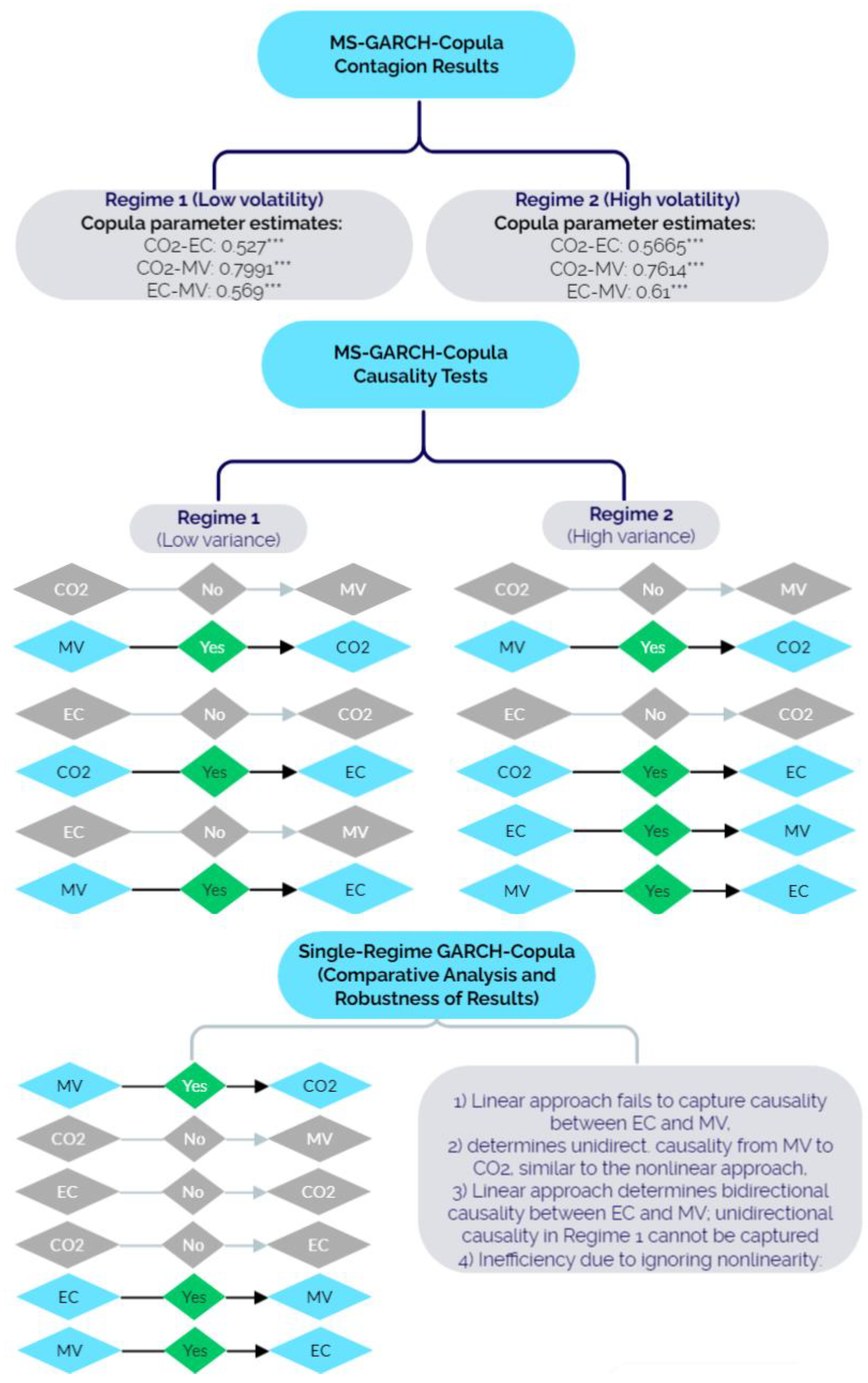
Copula Results
Regime 1			Regime 2
CO2-EC	CO2-MV	EC-MV	CO2-EC	CO2-MV	EC-MV
0.527 ***	0.7991 ***	0.569 ***	0.5665 ***	0.7614 ***	0.61 ***

¹ t statistics are reported in parentheses. ***, **, and * denote statistical significance at the 1%, 5% and 10% significance levels. LogL: log-likelihood, RMSE: root mean squared errors, MAE: mean absolute error, MAE: mean absolute error. ARCH-LM is the ARCH LM test statistic for which the LM test statistics are reported.

.

Before the interpretation of the parameter estimates for contagion, a set of measures should be evaluated to define the characteristics of each regime to be analyzed. The regime transition probabilities are reported for this purpose. P(st|st−1) is the conditional probability of the state at period t conditional on the state at period t – 1, and in the table, P(1|1) stands for P(st = 1|st−1 = 1). The persistence of each regime is dictated and depends on the regime-switching probability estimates. Similarly, P(2|2) designates P(st = 2|st−1 = 2). Both P(1|1) and P(2|2) are statistically significant at the 5% significance level. For all MS-GARCH marginal models modeling CO₂, EC, and MV series, the transition probability estimates are no less than 0.7, suggesting a strong level of persistence in each regime; however, P(1|1) > P(2|2), and the first regime is relatively more persistent for all variables except CO₂. Therefore, for EC and the MV, the second regime is more persistent, while it is the opposite for CO₂. However, it should be remembered that both regimes have a strong level of persistency. Since the standard error estimates are lower in Regime 1 relative to Regime 2 for all variables, Regime 1 is characterized as the low-variance or, in other words, low-volatility regime. Hence, Regime 2 indicates a relatively higher volatility regime for the MV, EC, and CO₂.

If the parameter estimates are evaluated, we observe distinct ARCH and GARCH parameter estimates in each regime, confirming asymmetry in volatility dynamics. In addition, the stability criterion, ARCH + GARCH < 1 is satisfied for each regime of the models for the MV, EC, and CO₂. Finally, the remaining unmodelled volatility is tested with ARCH-LM tests for each model, and we report the p-values in the last column. At a 5% significance level, the null hypothesis of no ARCH-type heteroskedasticity cannot be rejected, leading to findings suggesting that ARCH-type heteroskedasticity dynamics are effectively captured. The last column also reports various statistics including LogL, RMSE, and MAE, suggesting satisfactory results for the fit of the models. For contagion and tail dependence, the copula parameter estimates are given in the last two rows. The copula parameters are measures of tail dependence and are important measures of contagion. The copula parameter estimates in Regimes 1 and 2 are 0.527 and 0.5665 for the CO₂-EC pair, pointing at the strong degree of positive dependence and contagion between CO₂ emission concentration and energy consumption in both regimes, though relatively larger in the second regime, that is, the high-volatility regime. The CO₂-MV pair leads to an even larger degree of positive tail dependence of 0.7991 and 0.7614 in Regimes 1 and 2. For the EC-MV pair, the copula estimates are 0.56 in the low-volatility regime and 0.59 in the high-volatility regime. The results indicate a strong degree of contagion among all variables with close but varying magnitudes for regimes and provide support for positive associations. The significance of the coefficients and their sizes suggest a moderate level of tail dependence amid the metaverse and energy consumption and moderate to high levels of dependence between CO₂ emission concentration and the metaverse.

3.2.5. Nonlinear Causality Test Results with Regime-Switching and Copulae

MS-GARCH–Copula models are generalized to MS-GARCH–Copula Causality tests following Section 2. Test results are given in

Table 8. Nonlinear and regime-specific MS-GARCH–Copula Causality tests.

Direction of Causality under H1:	Regime 1	Causality?	Result:	Regime 2	Causality?	Result:
CO2→MV MV→CO2	1.00102 1	No	MV→CO2 (Unidirect.)	0.87728	No	MV→CO2 (Unidirect.)
	3.31528 **	Yes		3.62045 **	Yes
EC→CO2 CO2→EC	0.17533	No	CO2→EC (Unidirect.)	1.22553	No	CO2→EC (Unidirect.)
	2.74820 **	Yes		2.77701 **	Yes
MV→EC EC→MV	3.04436 **	Yes	MV→EC (Unidirect.)	2.94021 **	Yes	MV⇄EC (Bidirect.)
	1.40628	No		2.98736 **	Yes

¹ t statistics are reported. ** indicates statistical significance at the 1% significance level.

below for the regime-dependent causality tests that were conducted. The tests aim to examine and determine the direction of causality in each regime. Causality test results also provide a tool to produce policy recommendations.

The causality between the MV and CO₂ emission concentration test results is given in the first row for each regime. The test results indicate unidirectional causality from the MV to CO₂ in both the low- and high-volatility regimes. Since the causality in the opposite direction does not hold, the direction of causality is confirmed to be regime-indifferent. Causal tests given in the second row evaluate the causal links between EC and CO₂ emission concentration. The results confirm unidirectional causality in both regimes from CO₂ to EC. The last row reports the causality tests between the MV and EC, where the findings favored unidirectional causality from MV to EC in Regime 1. However, in the high-volatility regimes denoted as Regime 2, bidirectional causality could not be rejected. The results provide evidence of feedback effects in Regime 2 only, and no feedback effect exists from EC to the MV in the low-volatility regimes. Overall, this investigation suggests asymmetry in causality dynamics with varying test statistics and even differentiated results depending on the regime.

We aim to examine whether the findings obtained by asymmetric causality testing provided deviations from the non-regime-switching methods because of omitting the nonlinearity of the Markov-switching form. Due to the highly volatile nature of the series, linear Granger causality tests based on vector autoregressive (VAR) models would be inappropriate. Therefore, as a baseline model, we provided single-regime GARCH–Copula-Causality test results [43]. The results are given in

Table 9. Regime-independent single-regime GARCH–Copula Causality tests.

Direction of Causality under H1:	Test Statistic 1	Causality?	Result:
CO2→MV MV→CO2	0.51875	No	MV→CO2 (Unidirectional)
	2.51875 *	Yes
CO2→EC EC→CO2	1.11234	No	No causality
	0.74383	No
EC→MV MV→EC	8.63478 **	Yes	MV⇄EC (Bidirectional)
	9.91133 **	Yes

¹ t-statistics are reported. * and ** indicate statistical significance at the 5% and 1% significance levels, respectively.

.

According to the results reported in the first row of Table 9, unidirectional causality is confirmed from the MV to CO₂, similar to the Markov-switching version reported in Table 8. The second row of Table 9 reports the linear causality test results between CO₂ and EC and, accordingly, no causality exists among them. In contrast, our results in Table 8 suggested no causal link in Regime 1 only, but unidirectional causality from EC to CO₂ in Regime 2, the high-volatility regime. The last column of Table 9 is in line with Table 8’s last column, confirming the rejection of non-causality and acceptance of causality between the MV and EC. A summary of comparative results is reported in

Table 10. GARCH–Copula Causality tests: comparative results.

Direction of Causality:	MS-ARMA-GARCH Copula Causality		ARMA-GARCH-Copula Causality	Difference in Results?
	Regime 1	Regime 2	Single Regime
CO2→MV	MV→CO2 (Unidirectional)	MV→CO2 (Unidirectional)	MV→CO2	No
MV→CO2
CO2→EC	CO2→EP (Unidirectional)	CO2→EP (Unidirectional)	No causality between CO2 and EP	Yes
EC→CO2
EC→MV	MV→EP (Unidirectional)	MV⇄EP (Bidirectional)	MV⇄EP (Bidirectional)	Yes, but similar to Regime 2
MV→EC

.

3.3. Discussion with Comparisons to the Existent Literature

The results of the linear approach should be evaluated with caution since all variables exhibit nonlinear behavior, and omitting nonlinearity could lead to inefficiencies possibly with deviated directions causality.

Overall, the results indicate the effects of the metaverse on EC and CO₂. Here, we aim to compare such findings with the existing literature. However, the number of studies is limited. One reason is data availability. In terms of CO₂ and the MV, we found no studies with similar empirical investigations as our paper. In the neighboring literature, Ferreira et al. show positive and mid-to-high level dependence relationships for fintech, Bitcoin, and CO₂ emissions [60]. The effectiveness of nonlinear causality modeling through copulae with GARCH marginals is shown to be efficient for nonlinear relationships and series [43]. Compared with Kim et al.’s study, this study extends GARCH-copula to MS-type regime switching, and the findings confirm the nonlinear effects of the MV on EC and CO₂. Such effects are also shown to exist for different financial markets including the metaverse [41]. Non-fungible tokens (NFTs) are considered by some as a factor to integrate into the metaverse in the near future. Among the empirical research, few research papers point to NFT market volatility and transmissions to other markets. The dependence between NFT markets, its three sub-markets, and commodity and equity markets including gold and oil prices is shown with quantile cross-spectral coherency and quantile regression methods [61]. The NFT market is shown to be in relation to geopolitical risks and equity market volatility [61].

Our paper confirms the dependence between the MV and energy consumption in addition to a strong level of tail dependence with CO₂ emission concentration, a measure of air pollution, under distinct regimes. With a different method and data, Kshetri and Dwivedi suggest the MV could have carbon footprints, which could have environmental implications due to their energy requirements [14]. Another study is Zhao and You’s paper, which highlighted expectations for the consumer-side MV to contribute to environmental degradation [62]. These explanations focus on the technological adaptation level of the MV, and our study has a clear difference in terms of method and theory. While these studies focus on the level of MV technology and its effects on energy consumption, the unavailability of energy consumption directly from MV technology leads to an impossibility of empirical analysis. However, our paper provides a different aspect of the MV. We argue that MV companies have reached a considerable size in the stock market, so the fluctuations in MV stocks could have effects or associations between energy consumption and CO₂ emissions, and the results indicate such findings. In fact, the stock market size of the metaverse and its volatility have positive effects on both EC and CO₂; however, these results are evident as tail dependence, confirming contagion at lower and upper tails. Overall, there is a lack of empirical research on the nexus between the metaverse, EC, and CO₂ emission concentration, and an important reason is the availability of data, despite existing projections in the literature.

A limited amount of the literature follows a similar approach in the neighbor literature on cryptocurrencies. Syuhada et al. examine Mana and Theta metaverse cryptocurrencies using connectedness measures, and they highlight connectedness with proposed aggregate Value at Risk (VaR) and Expected Shortfall (ES) measures and copulae modeling [63]. Nonlinearity modeling is also shown to improve efficiency in dual rotor systems [64].

By putting forth nonlinear and heteroskedastic dynamics in the MV-EC-CO₂ nexus, our research provides an early empirical analysis with the hope of future work that utilizes new approaches after the availability of metaverse data at an aggregate level. Other than the data issue, this paper also contributes in terms of showing chaotic dynamics of the data analyzed. In the case of the dataset analyzed, this paper confirms that causality dynamics could be modeled with MS-GARCH–Copula–Causality, which allows for nonlinearity and regime-dependent contagion and causality relations.

4. Conclusions and Policy Recommendations

The assessment of the metaverse and its links to energy and the environment is of crucial importance. This paper aimed to fill the research gap regarding the examination of the metaverse, energy consumption, and CO₂ emission concentrations. The metaverse index utilized in this study comprises a large set of high-tech companies, and it is argued that the dataset characterized with nonlinearity, chaos, and fractionality in certain cases could be modeled with MS-GARCH–Copula and Causality methods for contagion and causality dynamics. Due to the characteristics determined with relevant tests for the data, such a setting is crucial to examine the tail-dependence and associations among metaverse stocks that are under the influence of metaverse technology fluctuations and shocks, possibly with contagion effects on energy consumption and global air pollution at the upper and lower tails of the dataset.

The nonlinearity and fractionality tests favored fractionality, nonlinearity, and long-term dependence in all series analyzed, which became especially evident for the volatility of all series analyzed. Further, chaotic structure, complexity and entropy could not be rejected in CO₂ emission concentrations, the metaverse, or energy consumption. These effects became more vital at the upper and lower tails of the distributions of data, characterized by two distinct regimes in this study, noted as the low- and high-volatility regimes, respectively. Further, fractionality was most evident in the CO₂ emissions concentrations.

Following the determination of chaotic and nonlinear processes in addition to fractionality and long-term dependence, the series were modeled with MS- GARCH–Copula and MS-GARCH-Copula–Causality methods in the modeling stage. The results and conclusions obtained from the MS-GARCH–Copula Causality method are summarized in Figure 1, followed by the results gathered from the GARCH–Copula Causality, which is the single-regime approach. Compared with the former, the latter omits nonlinearity; however, this model deviates from traditional Granger causality tests since it specifically focuses on controlling heteroskedasticity in the series analyzed.

The nonlinear MS-GARCH–Copula and Causality methods provided important insights into two distinct regimes characterized as low- and high-volatility regimes, and according to our findings, tail dependence and contagion existed in both regimes. The level of dependence measured with copula parameter estimates ranged between 0.53 and 0.79 depending on the regime, which pointed to a moderate to high level of positive association between each series, confirming the contagion and tail-dependence between the metaverse, energy consumption, and CO₂.

After the determination of tail dependence with copula parameters, the direction of causality was determined with the utilized nonlinear approaches. The findings indicated unidirectional causal links from the metaverse to energy consumption, from the metaverse to CO₂, and from CO₂ to energy consumption in both the low- and high-volatility regimes. Further, unidirectional causality existed from the metaverse to CO₂, while the relationship became bidirectional in Regime 2, indicating a cyclical pattern of causality with feedback effects in the high-volatility regime. It is evident that during more turbulent periods, the connection between the metaverse and energy consumption is subject to a cyclical self-feeding pattern, and caution is needed for their environmental effects. Hence, in the future, unless the energy dependence of the metaverse can be solved, the environmental effects could be more harmful. Overall, a not-so-favorable result is a positive association between metaverse stocks and EC and CO₂ emissions no matter the regime type. Given the strong level of association, the upward trend in the metaverse necessitates urgent policies to encourage energy-efficient and cleaner technological advancements to reduce the footprint of such technologies. Lastly, the findings were compared with the single-regime GARCH-Copula Causality results for comparative and robustness purposes. Ignoring nonlinearity in the series could lead to deviations in the direction of causality, therefore resulting in inefficiencies in policy applications aiming at controlling the metaverse’s effects on energy use and the environmental degradation.

Figure 1. A summary of the conclusions and empirical results. Note. *** indicates statistical significance at the 1% significance level. The findings of our study, combined with the existing literature, have enabled us to generate a comprehensive set of policy recommendations. The trajectory of the metaverse phenomenon will play a pivotal role in mitigating its environmental impacts. Analogous to the pervasive rise of the internet, e-commerce, and digital devices over the past two to three decades, the metaverse harbors the potential for substantial environmental repercussions unless its energy policies undergo careful reevaluation. As the metaverse gains broader societal accessibility, akin to the ubiquitous presence of the internet and smart devices in contemporary lives, the escalating energy demands associated with metaverse activities will inevitably lead to heightened emissions. To curtail the pace and magnitude of these adverse effects, implementation of intelligent automation technologies to enhance energy efficiency, prioritizing the adoption of renewable energy sources to reduce reliance on fossil fuels and mitigate GHG, e-waste management, and encouragement of recycling in metaverse companies and the metaverse community is of vital importance. In addition, emphasizing the use of eco-friendly materials and efficient recycling methods is important, including recovering resources from used equipment, for example, batteries.

Figure 1. A summary of the conclusions and empirical results. Note. *** indicates statistical significance at the 1% significance level. The findings of our study, combined with the existing literature, have enabled us to generate a comprehensive set of policy recommendations. The trajectory of the metaverse phenomenon will play a pivotal role in mitigating its environmental impacts. Analogous to the pervasive rise of the internet, e-commerce, and digital devices over the past two to three decades, the metaverse harbors the potential for substantial environmental repercussions unless its energy policies undergo careful reevaluation. As the metaverse gains broader societal accessibility, akin to the ubiquitous presence of the internet and smart devices in contemporary lives, the escalating energy demands associated with metaverse activities will inevitably lead to heightened emissions. To curtail the pace and magnitude of these adverse effects, implementation of intelligent automation technologies to enhance energy efficiency, prioritizing the adoption of renewable energy sources to reduce reliance on fossil fuels and mitigate GHG, e-waste management, and encouragement of recycling in metaverse companies and the metaverse community is of vital importance. In addition, emphasizing the use of eco-friendly materials and efficient recycling methods is important, including recovering resources from used equipment, for example, batteries.

One could argue that many dominant factors that exist, which affect CO₂ emissions and its concentration, the metaverse, and Bitcoin’s energy consumption could have limited effects comparatively. This study does not have such a proposal; however, it is a pivotal study that directs attention to recent metaverse technologies in addition to Bitcoin’s energy consumption. Further, as discussed in Section 1 and Section 2, the energy consumption of such technologies and their environmental effects are shown to amount to those of a set of countries. This paper suggests that close attention is needed for such new technologies, and the findings confirm their effects are becoming evident on the air pollution concentration.

The findings pointed to fractionality, chaos, and nonlinearity in all series. The modeling of the metaverse, Bitcoin’s energy consumption, and air pollution with daily datasets should aim at integrating these characteristics of data in future studies. In this respect, this study confirmed tail dependence and contagion with asymmetric copula parameters in addition to causality among the metaverse, energy consumption, and CO₂ emissions. Hence, this study is pivotal in highlighting the implications of the metaverse and Bitcoin’s energy consumption and their impacts on global CO₂ emissions concentrations.

Two sets of policies could be generated. First, on the metaverse company side, to mitigate CO₂ emissions, decision-makers should aim to reduce the carbon footprint of the metaverse drastically in manufacturing. However, there is a policy gap for such a commitment, and economic incentives could be generated by a set of policies including carbon tax and carbon subsidies and campaigns for consumer awareness. Second, on the national level, policies should aim to improve energy efficiency, renewable energy investments, and carbon capture technologies to support the mitigation of energy consumption and the environment effects of future metaverse technologies.

References

- Schaffer, W.M. Order and Chaos in Ecological Systems. Ecology 1985, 66, 93–106. [Google Scholar] [CrossRef]
- Lorenz, E.N. Deterministic Nonperiodic Flow. J. Atmos. Sci. 1963, 20, 130–141. [Google Scholar] [CrossRef]
- Li, I.-F.; Biswas, P.; Islam, S. Estimation of the Dominant Degrees of Freedom for Air Pollutant Concentration Data: Applications to Ozone Measurements. Atmos. Environ. 1994, 28, 1707–1714. [Google Scholar] [CrossRef]
- Raga, G.B.; Le Moyne, L. On the Nature of Air Pollution Dynamics in Mexico City—I. Nonlinear Analysis. Atmos. Environ. 1996, 30, 3987–3993. [Google Scholar] [CrossRef]
- Kumar, U.; Prakash, A.; Jain, V.K. Characterization of Chaos in Air Pollutants: A Volterra–Wiener–Korenberg Series and Numerical Titration Approach. Atmos. Environ. 2008, 42, 1537–1551. [Google Scholar] [CrossRef]
- Lee, C.-K.; Lin, S.-C. Chaos in Air Pollutant Concentration (APC) Time Series. Aerosol Air Qual. Res. 2008, 8, 381–391. [Google Scholar] [CrossRef]
- Yu, B.; Huang, C.; Liu, Z.; Wang, H.; Wang, L. A Chaotic Analysis on Air Pollution Index Change over Past 10 Years in Lanzhou, Northwest China. Stoch. Environ. Res. Risk Assess. 2011, 25, 643–653. [Google Scholar] [CrossRef]
- Bildirici, M. Chaotic Dynamics on Air Quality and Human Health: Evidence from China, India, and Turkey. Nonlinear Dyn. Psychol. Life Sci. 2021, 25, 207–236. [Google Scholar]
- Ucan, Y.; Bildirici, M. Air Temperature Measurement Based on Lie Group SO(3). Therm. Sci. 2022, 26, 3089–3095. [Google Scholar] [CrossRef]
- Rimol, M. Gartner Predicts 25% of People Will Spend at Least One Hour per Day in the Metaverse by 2026. Available online: https://www.gartner.com/en/newsroom/press-releases/2022-02-07-gartner-predicts-25-percent-of-people-will-spend-at-least-one-hour-per-day-in-the-metaverse-by-2026 (accessed on 13 June 2023).
- Wiggers, K. The Environmental Impact of the Metaverse. Available online: https://venturebeat.com/data-infrastructure/the-environmental-impact-of-the-metaverse/ (accessed on 13 June 2023).
- Morris, C. Citi Says Metaverse Could Be Worth $13 Trillion by 2030. Fortune, 1 April 2022. [Google Scholar]
- Stoll, C.; Gallersdörfer, U.; Klaaßen, L. Climate Impacts of the Metaverse. Joule 2022, 6, 2668–2673. [Google Scholar] [CrossRef]
- Kshetri, N.; Dwivedi, Y.K. Pollution-Reducing and Pollution-Generating Effects of the Metaverse. Int. J. Inf. Manag. 2023, 69, 102620. [Google Scholar] [CrossRef]
- Huang, J.; O’Neill, C.; Tabuchi, H. Bitcoin Uses More Electricity Than Many Countries: How Is That Possible? The New York Times, 3 September 2021. [Google Scholar]
- Iberdrola.com. What Are Green Cryptocurrencies and Why Are They Important? Available online: https://www.iberdrola.com/sustainability/green-cryptocurrencies (accessed on 13 March 2023).
- Malfuzi, A.; Mehr, A.S.; Rosen, M.A.; Alharthi, M.; Kurilova, A.A. Economic Viability of Bitcoin Mining Using a Renewable-Based SOFC Power System to Supply the Electrical Power Demand. Energy 2020, 203, 117843. [Google Scholar] [CrossRef]
- De Vries, A. Bitcoin’s Energy Consumption Is Underestimated: A Market Dynamics Approach. Energy Res. Soc. Sci. 2020, 70, 101721. [Google Scholar] [CrossRef]
- Digiconomist Bitcoin Energy Consumption Index—Digiconomist. Available online: https://digiconomist.net/bitcoin-energy-consumption (accessed on 14 March 2023).
- Zhang, C.; Liu, S. Meta-Energy: When Integrated Energy Internet Meets Metaverse. IEEE/CAA J. Autom. Sin. 2023, 10, 580–583. [Google Scholar] [CrossRef]
- Bildirici, M. The Chaotic Behavior among the Oil Prices, Expectation of Investors and Stock Returns: TAR-TR-GARCH Copula and TAR-TR-TGARCH Copula. Pet. Sci. 2019, 16, 217–228. [Google Scholar] [CrossRef]
- Shannon, C.E. A Mathematical Theory of Communication. Bell Syst. Tech. J. 1948, 27, 379–423. [Google Scholar] [CrossRef]
- Lo, A.W. Long-Term Memory in Stock Market Prices. Econometrica 1991, 59, 1279. [Google Scholar] [CrossRef]
- Geweke, J.; Porter-Hudak, S. The Estimation and Application of Long Memory Time Series Models. J. Time Ser. Anal. 1983, 4, 221–238. [Google Scholar] [CrossRef]
- Robinson, P.M.; Henry, M. Higher-Order Kernel Semiparametric M-Estimation of Long Memory. J. Econom. 2003, 114, 1–27. [Google Scholar] [CrossRef]
- Panas, E.; Ninni, V. Are Oil Markets Chaotic? A Non-Linear Dynamic Analysis. Energy Econ. 2000, 22, 549–568. [Google Scholar] [CrossRef]
- Gaspard, P.; Briggs, M.E.; Francis, M.K.; Sengers, J.V.; Gammon, R.W.; Dorfman, J.R.; Calabrese, R.V. Experimental Evidence for Microscopic Chaos. Nature 1998, 394, 865–868. [Google Scholar] [CrossRef]
- Pincus, S. Approximate Entropy (ApEn) as a Complexity Measure. Chaos Interdiscip. J. Nonlinear Sci. 1995, 5, 110–117. [Google Scholar] [CrossRef]
- Rosenstein, M.T.; Collins, J.J.; De Luca, C.J. A Practical Method for Calculating Largest Lyapunov Exponents from Small Data Sets. Phys. D Nonlinear Phenom. 1993, 65, 117–134. [Google Scholar] [CrossRef]
- Zhong, Z.-Q.; Wu, Z.-M.; Xia, G.-Q. Experimental Investigation on the Time-Delay Signature of Chaotic Output from a 1550 Nm VCSEL Subject to FBG Feedback. Photonics Res. 2017, 5, 6–10. [Google Scholar] [CrossRef]
- Savi, M.A. Chaos and Order in Biomedical Rhythms. J. Braz. Soc. Mech. Sci. Eng. 2005, 27, 157–169. [Google Scholar] [CrossRef]
- Havrda, J.; Charvât, F. Quantification Method of Classification Processes Concept of Structural α-Entropy. Kybernetica 1967, 3, 30–35. [Google Scholar]
- Tsallis, C. Possible Generalization of Boltzmann-Gibbs Statistics. J. Stat. Phys. 1988, 52, 479–487. [Google Scholar] [CrossRef]
- Kaspar, F.; Schuster, H.G. Easily Calculable Measure for the Complexity of Spatiotemporal Patterns. Phys. Rev. A 1987, 36, 842–848. [Google Scholar] [CrossRef] [PubMed]
- Mandelbrot, B.B.; Wallis, J.R. Robustness of the Rescaled Range R/S in the Measurement of Noncyclic Long Run Statistical Dependence. Water Resour. Res. 1969, 5, 967–988. [Google Scholar] [CrossRef]
- Brock, W.A.; Dechert, W.D.; Scheinkman, J.A. A Test for Independence Based on the Correlation Dimension; University of Wisconsin, Social Systems Research Unit: Madison, WI, USA, 1987. [Google Scholar]
- Broock, W.A.; Scheinkman, J.A.; Dechert, W.D.; LeBaron, B. A Test for Independence Based on the Correlation Dimension. Econom. Rev. 1996, 15, 197–235. [Google Scholar] [CrossRef]
- White, H. A Heteroskedasticity-Consistent Covariance Matrix Estimator and a Direct Test for Heteroskedasticity. Econometrica 1980, 48, 817–838. [Google Scholar] [CrossRef]
- Engle, R.F. Autoregressive Conditional Heteroscedasticity with Estimates of the Variance of United Kingdom Inflation. Econometrica 1982, 50, 987–1007. [Google Scholar] [CrossRef]
- Bildirici, M.E.; Salman, M.; Ersin, Ö.Ö. Nonlinear Contagion and Causality Nexus between Oil, Gold, VIX Investor Sentiment, Exchange Rate and Stock Market Returns: The MS-GARCH Copula Causality Method. Mathematics 2022, 10, 4035. [Google Scholar] [CrossRef]
- Bildirici, M.E. Chaos Structure and Contagion Behavior between COVID-19, and the Returns of Prices of Precious Metals and Oil: MS-GARCH-MLP Copula. Nonlinear Dyn. Psychol. Life Sci. 2022, 26, 209–230. [Google Scholar]
- Bildirici, M.E.; Sonustun, B. Chaotic Behavior in Gold, Silver, Copper and Bitcoin Prices. Resour. Policy 2021, 74, 102386. [Google Scholar] [CrossRef]
- Kim, J.M.; Lee, N.; Hwang, S.Y. A Copula Nonlinear Granger Causality. Econ. Model. 2020, 88, 420–430. [Google Scholar] [CrossRef]
- Bildirici, M.; Ersin, Ö. Modeling Markov Switching ARMA-GARCH Neural Networks Models and an Application to Forecasting Stock Returns. Sci. World J. 2014, 2014, 497941. [Google Scholar] [CrossRef]
- Bildirici, M.E. Economic Growth and Electricity Consumption: MS-VAR and MS-Granger Causality Analysis. OPEC Energy Rev. 2013, 37, 447–476. [Google Scholar] [CrossRef]
- Bollerslev, T. Generalized Autoregressive Conditional Heteroskedasticity. J. Econom. 1986, 31, 307–327. [Google Scholar] [CrossRef]
- Henneke, J.S.; Rachev, S.T.; Fabozzi, F.J.; Nikolov, M. MCMC-Based Estimation of Markov Switching ARMA–GARCH Models. Appl. Econ. 2011, 43, 259–271. [Google Scholar] [CrossRef]
- Francq, C.; Zakoïan, J.-M. Stationarity of Multivariate Markov–Switching ARMA Models. J. Econom. 2001, 102, 339–364. [Google Scholar] [CrossRef]
- Kim, C.J. Dynamic Linear Models with Markov-Switching. J. Econom. 1994, 60, 1–22. [Google Scholar] [CrossRef]
- Granger, C.W.J. Investigating Causal Relations by Econometric Models and Cross-Spectral Methods. Econometrica 1969, 37, 424–438. [Google Scholar] [CrossRef]
- Zhu, K.; Yamaka, W.; Sriboonchitta, S. Multi-Asset Portfolio Returns: A Markov Switching Copula-Based Approach. Thai J. Math. 2016, 183–200. [Google Scholar]
- Nalatore, H.; Sasikumar, N.; Rangarajan, G. Effect of Measurement Noise on Granger Causality. Phys. Rev. E Stat. Nonlinear Soft Matter Phys. 2014, 90, 062127. [Google Scholar] [CrossRef]
- Lee, T.-H.; Yang, W. Granger-Causality in Quantiles between Financial Markets: Using Copula Approach. Int. Rev. Financ. Anal. 2014, 33, 70–78. [Google Scholar] [CrossRef]
- Dickey, D.A.; Fuller, W.A. Distribution of the Estimators for Autoregressive Time Series With a Unit Root. J. Am. Stat. Assoc. 1979, 74, 427. [Google Scholar] [CrossRef]
- Kapetanios, G.; Shin, Y.; Snell, A. Testing for a Unit Root in the Nonlinear STAR Framework. J. Econom. 2003, 112, 359–379. [Google Scholar] [CrossRef]
- Kwiatkowski, D.; Phillips, P.C.B.; Schmidt, P.; Shin, Y. Testing the Null Hypothesis of Stationarity against the Alternative of a Unit Root: How Sure Are We That Economic Time Series Have a Unit Root? J. Econom. 1992, 54, 159–178. [Google Scholar] [CrossRef]
- Sivakumar, B. Chaos Theory in Hydrology: Important Issues and Interpretations. J. Hydrol. 2000, 227, 1–20. [Google Scholar] [CrossRef]
- Kaplan, D.T.; Furman, M.I.; Pincus, S.M.; Ryan, S.M.; Lipsitz, L.A.; Goldberger’, A.L. Aging and the Complexity of Cardiovascular Dynamics. Biophys. J. 1991, 59, 945–949. [Google Scholar] [CrossRef] [PubMed]
- Richman, J.S.; Randall Moorman, J.; Randall, J.; Physi, M. Physiological Time-Series Analysis Using Approximate Entropy and Sample Entropy. Am. J. Physiol. Heart Circ. Physiol. 2000, 278, 2039–2049. [Google Scholar] [CrossRef] [PubMed]
- Ferreira, P.; Dionísio, A.; Movahed, S.M.S. Assessment of 48 Stock Markets Using Adaptive Multifractal Approach. Phys. A Stat. Mech. Its Appl. 2017, 486, 730–750. [Google Scholar] [CrossRef]
- Urom, C.; Ndubuisi, G.; Guesmi, K. Dynamic Dependence and Predictability between Volume and Return of Non-Fungible Tokens (NFTs): The Roles of Market Factors and Geopolitical Risks. Financ. Res. Lett. 2022, 50, 103188. [Google Scholar] [CrossRef]
- Zhao, N.; You, F. The Growing Metaverse Sector Can Reduce Greenhouse Gas Emissions by 10 Gt CO2e in the United States by 2050. Energy Environ. Sci. 2023, 16, 2382–2397. [Google Scholar] [CrossRef]
- Syuhada, K.; Tjahjono, V.; Hakim, A. Dependent Metaverse Risk Forecasts with Heteroskedastic Models and Ensemble Learning. Risks 2023, 11, 32. [Google Scholar] [CrossRef]
- Yu, P.; Hou, L.; Wang, C.; Chen, G. Insights into the Nonlinear Behaviors of Dual-Rotor Systems with Inter-Shaft Rub-Impact under Co-Rotation and Counter-Rotation Conditions. Int. J. Non-Linear Mech. 2022, 140, 103901. [Google Scholar] [CrossRef]