Finite Difference and Chebyshev Collocation for Time-Fractional and Riesz Space Distributed-Order Advection–Diffusion Equation with Time-Delay

Abstract

In this paper, we have established a numerical method for a class of time-fractional and Riesz space distributed-order advection–diffusion equation with time-delay. Firstly, we transform the Riesz space distributed-order derivative term of the diffusion equation into multi-term fractional derivatives by using the Gauss quadrature formula. Secondly, we discretize time by using second-order finite differences, discretize space by using second kind Chebyshev polynomials, and convert the multi-term fractional equation to a system of algebraic equations. Finally, we solve the algebraic equations by the iterative method, and prove the stability and convergence. Moreover, relevant examples are shown to verify the validity of our algorithm.

1. Introduction

In recent years, the study of partial differential equations has played a crucial role in understanding and imitating complex physical phenomena [1,2,3,4]. Among them, the research on advection–diffusion equations has been extensively studied in various fields such as environmental science, biology, and engineering.

As we gain a deeper understanding of physical processes, it has become evident that the traditional integer-order differential equations often fail to accurately describe certain phenomena with memory effects, long-range interactions, and non-local behaviors. Fractional calculus, which involves derivatives and integrals of non-integer orders, has emerged as a powerful tool to address these challenges. Time-fractional derivatives can capture the memory and hereditary properties of a system [5,6,7,8,9,10], while space distributed-order derivatives can account for the heterogeneity and non-uniformity of the medium.

Caputo first proposed the distributed-order differential equations [11,12]. As time goes by, there have been some reports written concerning the theoretical and numerical solution research of distributed-order partial differential equations [13,14,15,16,17,18,19,20,21,22,23,24,25,26,27]. Explicit strong solutions and stochastic simulations of the distributional-order time-fractional order diffusion equation on bounded domains were given by Meerschaert et al. with Dirichlet boundary conditions [13]. Atanackovic et al. proved the exsitence of the solution to the Cauchy problem for the time distributed-order diffusion equation as well as to calculate it [14]. For more theoretical studies of distributed-order partial differential equations, see [15,16,17,18,19,20]. In addition, many results have been obtained on the numerical solutions of distributed-order partial differential equations. Ye et al. derived a compact difference scheme for the distributed-order time-fractional diffusion wave equation and proved that the compact difference scheme is unconditionally stable and convergent [22]. Chen et al. obtained a novel fourth-order accurate difference method for the distributed-order Riesz space fractional diffusion equation in one-dimensional (1D) and two-dimensional (2D) cases [23]. Li et al. proposed a novel finite volume method for the Riesz space distributed-order advection diffusion equation and proved that the Crank–Nicolson scheme is unconditionally stable and convergent with second-order accuracy [24]. Zhang et al. proposed a Crank–Nicolson alternating-direction implicit (ADI) Galerkin–Legendre spectral scheme for the two-dimensional Riesz spatial distribution-order advection diffusion equation [25]. They also proposed an alternating direction implicit (ADI) Legendre–Laguerre spectral scheme for the two-dimensional time distributed-order diffusion-wave equation on a semi-infinite domain [26]. Niu et al. presented an efficient numerical algorithm for solving the nonlinear distributed-order fractional Sobolev model appearing in porous media, which combines the fourth-order compact difference scheme (CDS) in space with the fast time two-mesh (TT-M) FBN—$\mathsf{\theta }$ method [27]. In addition to fractional derivatives, the consideration of delay terms in equations is also of great significance. In many real-world systems, the current state often depends not only on current conditions but also on past states. The introduction of delay terms enables us to better model systems with time delays, such as biological processes with growth lags, chemical reactions with induction periods, and communication systems with signal delays. The theoretical analysis and numerical solutions of fractional-order delay differential equations have yielded many results [28,29,30,31,32,33,34,35,36].

Based on existing research results, Javidi and Heris studied the space distributed-order advection–diffusion equation with delay using the fractional backward differentiation formula (FBDF) and Grünwald difference method on the basis of [24]. They have also proved that the Crank–Nicolson scheme is conditionally stable and has second-order convergence accuracy. Meanwhile, regarding the spectral collocation method, Sweilam [37] and Agarwal [38] et al. proposed a configuration method with higher accuracy, mainly used to solve numerical solutions of linear fractional convection dispersion equations and fractional diffusion equations. In 2021, Sweilam [39] et al. proposed a spectral collocation method combining Vieta-fibonacci polynomials and non-standard finite differences for fractional -order convection-dispersion equations on the basis of paper [37]. Saw and Kumar used the spectral collocation method, which combined the second kind Chebyshev polynomials with finite difference to study the space fractional-order advection diffusion equation [40]. Ali Shah et al. presented a highly accurate method for the numerical solution of the advection—diffusion equation of fractional-order [41]. We aim to draw on the ideas in [40] and propose a novel spectral collocation method that integrates the second kind Chebyshev polynomial with second-order finite difference. Then, we will apply the novel spectral collocation method to study the time-fractional and Riesz space distributed-order advection–diffusion equation with time-delay, thereby breaking through the limitations of existing research methods and generalizing the results in [24].

Motivated by the above analysis, this paper employs the novel spectral collocation method to investigate the following time-fractional and Riesz space distributed-order advection–diffusion equation with time-delay:

$${}_0{}^{C}D_t^{\gamma }u(x,t)={\int }_1^2{P}_1\left(\alpha \right){\displaystyle \frac{{\partial }^{\alpha }u(x,t)}{{\partial \left|x\right|}^{\alpha }}}d\alpha +{\int }_0^1{P}_2\left(\beta \right){\displaystyle \frac{{\partial }^{\beta }u(x,t)}{{\partial \left|x\right|}^{\beta }}}d\beta +ru(x,t-\mu )+f(x,t),$$

(1)

with initial and boundary conditions:

$$u(x,t)=g(x,t),-\mu \le t\le 0,0\le x\le L,$$

(2)

$$u(0,t)=0,u(L,t)=0,0\le t\le T,$$

(3)

where $1<\alpha <2$, $0<\beta <1$, $0<\gamma \le 1$, $\mu >0$, $r\ge 0$, and $P_1\left(\alpha \right)$, $P_2\left(\beta \right)$ are non-negative weight functions satisfying the conditions

$$P_1\left(\alpha \right)\ge 0,0<{\int }_1^2{P}_1\left(\alpha \right)d\alpha <\infty ,$$

$$P_2\left(\beta \right)\ge 0,0<{\int }_0^1{P}_2\left(\beta \right)d\beta <\infty .$$

When $r=0$, Equation (1) will be a Riesz space distributed-order advection–diffusion equation without delay. In addition, the order of the advection is close to 1, and here we assume that $P_2\left(\beta \right)$ disappears outside the interval (1/2,1).

Moreover, in the literature [24,35,42], the Riesz space distributed-order derivative is approximated via the midpoint quadrature formula. Owing to the Gauss quadrature formula having superior accuracy compared to the midpoint quadrature formula, we consider the Gauss quadrature to approximate the Riesz space distributed-order derivative. For the general Riesz space distributed-order derivative ${\int }_{{\alpha }_{min}}^{{\alpha }_{max}}P\left(\alpha \right){\displaystyle \frac{{\partial }^{\alpha }u}{{\partial \left|x\right|}^{\alpha }}}d\alpha$, when the weight function $P\left(\alpha \right)$ is smooth, we can apply the Legendre-Gauss quadrature to approximate. When the weight function $P\left(\alpha \right)$ has weak singularities, we can rewrite the Riesz space distributed-order derivative

$${\int }_{{\alpha }_{min}}^{{\alpha }_{max}}P\left(\alpha \right){\displaystyle \frac{{\partial }^{\alpha }u}{{\partial \left|x\right|}^{\alpha }}}\omega {\omega }^{-1}d\alpha ,\omega ={(\alpha -{\alpha }_{min})}^a{({\alpha }_{max}-\alpha )}^b,(a,b)>-1,$$

where $\omega$ is a suitable weight function such that $P\left(\alpha \right){\displaystyle \frac{{\partial }^{\alpha }u}{{\partial \left|x\right|}^{\alpha }}}\omega$ is more smooth than $P\left(\alpha \right){\displaystyle \frac{{\partial }^{\alpha }u}{{\partial \left|x\right|}^{\alpha }}}$. Therefore, the Jacobi Gauss quadrature method is used to approximate the above integral. In other words, the Gauss quadrature formula allows for high accuracy for smooth and non-smooth weight functions.

The rest of this paper is organized as follows. In Section 2, we give the definition and properties of fractional calculus and Chebyshev polynomials, and derive approximate formulas for derivatives of the Riesz fractional-order. In Section 3, we give the errors analysis. In Section 4, we give the numerical scheme of the time and spatial discretization. In Section 5, we prove the stability and convergence of the numerical scheme. In Section 6, we give some numerical results to verify the validity and accuracy of our method.

2. Preliminaries and Necessary Mathematical Tools

2.1. Riesz Fractional Derivatives

Definition 1 

([25]). The Riesz fractional operators are defined by

$${\displaystyle \frac{{\partial }^{\alpha }u(x,t)}{{\partial \left|x\right|}^{\alpha }}}=c_{\alpha }({}_{\mathit{RL}}D_{a,x}^{\alpha }u(x,t)+{}_{\mathit{RL}}D_{x,b}^{\alpha }u(x,t)),$$

where $c_{\alpha }=-{\displaystyle \frac{1}{2cos(\alpha \pi /2)}}.$ For $n-1<\alpha <n,n\in \mathbb{N}$, the operators ${}_{\mathit{RL}}D_{a,x}^{\alpha }$ and ${}_{\mathit{RL}}D_{x,b}^{\alpha }$ are defined as

$${}_{\mathit{RL}}D_{a,x}^{\alpha }u(x,t)={\displaystyle \frac{{\partial }^n}{\partial x^n}}\left[D_{a,x}^{-(n-\alpha )}u(x,t)\right]={\displaystyle \frac{1}{\Gamma (n-\alpha )}}{\displaystyle \frac{{\partial }^n}{\partial x^n}}{\int }_a^x{(x-s)}^{n-\alpha -1}u(s,t)ds,$$

$${}_{\mathit{RL}}D_{x,b}^{\alpha }u(x,t)={(-1)}^n{\displaystyle \frac{{\partial }^n}{\partial x^n}}\left[D_{x,b}^{-(n-\alpha )}u(x,t)\right]={\displaystyle \frac{{(-1)}^n}{\Gamma (n-\alpha )}}{\displaystyle \frac{{\partial }^n}{\partial x^n}}{\int }_x^b{(s-x)}^{n-\alpha -1}u(s,t)ds.$$

Moreover, using Definition 1 to obtain the fractional derivative of the constant function C and polynomials $x^k$ as follows

$$D^{\alpha }C={\displaystyle \frac{x^{-\alpha }}{\Gamma (1-\alpha )}},C \mathrm{is} \mathrm{a} \mathrm{constant},$$

$${}_{a}D_x^{\alpha }{(x-a)}^k={\displaystyle \frac{\Gamma (k+1)}{\Gamma (k+1-\alpha )}}{(x-a)}^{k-\alpha },k>-1,x\in [a,b],$$

(4)

$${}_{x}D_b^{\alpha }{(b-x)}^k={\displaystyle \frac{\Gamma (k+1)}{\Gamma (k+1-\alpha )}}{(b-x)}^{k-\alpha },k>-1,x\in [a,b].$$

(5)

2.2. Chebyshev Polynomials of the Second Kind

Definition 2 

([43]). The Chebyshev polynomials are very well-known polynomials that are defined in the interval $[-1,1]$ by the relation

$$T_n\left(x\right)={\displaystyle \frac{sin(n+1)\theta }{sin\theta }}$$

of degree n in x, where $x=cos\left(\theta \right)$ and $\theta \in [0,\pi ]$.

The $T_n\left(x\right)$ are generated by the fundamental recurrence relations

$$T_{n+1}\left(x\right)=2x{T}_n\left(x\right)-T_{n-1}\left(x\right),n=1,2,\cdots ,$$

with defined values

$$T_0\left(x\right)=1,T_1\left(x\right)=2x.$$

$T_n\left(x\right)$ are orthogonal with respect to the weight function $w\left(x\right)$,

$$\begin{array}{cc}\hfill 〈T_n\left(x\right),T_m\left(x\right)〉& ={\int }_{-1}^1\omega \left(x\right)T_n\left(x\right)T_m\left(x\right)dx\hfill \\ \hfill & =\left\{\begin{array}{cc}0,\hfill & n\ne m,\hfill \\ {\displaystyle \frac{\pi }{2}},\hfill & n=m\ne 0,\hfill \end{array}\right.\hfill \end{array}$$

where $w\left(x\right)=\sqrt{(1-x^2)}$. Furthermore, $T_n\left(x\right)$ can also be expressed in the form of a power series

$$T_n\left(x\right)=\sum _{i=0}^{\lceil {\displaystyle \frac{n}{2}}\rceil }{(-1)}^i{2}^{n-2i}{\displaystyle \frac{\Gamma (n-i+1)}{\Gamma (i+1)\Gamma (n-2i+1)}}{x}^{n-2i},n\in {\mathbb{Z}}^{+}.$$

Definition 3 

([40]). The shifted Chebyshev polynomials of degree n on the domain $[0,1]$ are defined as follows

$$T_n^{*}\left(x\right)=T_n(2x-1).$$

The shifted Chebyshev polynomials are orthogonal polynomials with the weight function $w\left(x\right)$,

$$\begin{array}{cc}\hfill 〈T_n^{*}\left(x\right),T_m^{*}\left(x\right)〉& ={\int }_0^1\omega \left(x\right)T_n^{*}\left(x\right)T_m^{*}\left(x\right)dx\hfill \\ \hfill & =\left\{\begin{array}{cc}0,\hfill & n\ne m,\hfill \\ {\displaystyle \frac{\pi }{8}},\hfill & n=m\ne 0,\hfill \end{array}\right.\hfill \end{array}$$

(6)

where $w\left(x\right)=\sqrt{x-x^2}$ is the weight function. The fundamental recurrence relation of second kind shifted Chebyshev polynomials is defined as:

$$T_{n+1}^{*}\left(x\right)=2(2x-1)T_n^{*}\left(x\right)-T_{n-1}^{*}\left(x\right),n=1,2,\cdots ,$$

with the initial conditions

$$T_0^{*}\left(x\right)=1,T_1^{*}\left(x\right)=4x-2.$$

Furthermore, the shifted Chebyshev’s power series has the form

$$T_n^{*}\left(x\right)=\sum _{i=0}^n{(-1)}^i{2}^{2n-2i}{\displaystyle \frac{\Gamma (2n-i+2)}{\Gamma (i+1)\Gamma (2n-2i+2)}}{x}^{n-i},n\in {\mathbb{Z}}^{+},$$

(7)

or

$$T_n^{*}\left(x\right)=\sum _{i=0}^n{(-1)}^{n-i}{2}^{2i}{\displaystyle \frac{\Gamma (n+i+2)}{\Gamma (n-i+1)\Gamma (2i+2)}}{x}^i,n\in {\mathbb{Z}}^{+}.$$

(8)

Let $y\left(x\right)$ be square integrable function in $[0,1]$, the function $y\left(x\right)$ can be expanded into a power series of $T_n^{*}\left(x\right)$ as follows:

$$y\left(x\right)=\sum _{i=0}^{\infty }{\lambda }_i{T}_i^{*}\left(x\right).$$

(9)

Via the approximation theory, the terms of the series in Equation (9) are truncated to have only $n+1$ terms as follows:

$$y_n\left(x\right)=\sum _{i=0}^n{\lambda }_i{T}_i^{*}\left(x\right),$$

(10)

where the expansion coefficients ${\lambda }_i(i=0,1,2,\cdots )$ are unknown, which are defined as:

$${\lambda }_i={\displaystyle \frac{8}{\pi }}{\int }_0^{1}y\left(x\right)\sqrt{x-x^2}{T}_i^{*}\left(x\right)dx.$$

(11)

2.3. An Approximation Formula for Riesz Fractional Derivation

Theorem 1. 

Use $T_n^{*}\left(x\right)$ to express the approximate solution $y_n\left(x\right)$ of the main problem (1). And assume that $\alpha >0$. Then,

$${\displaystyle \frac{{\partial }^{\alpha }{y}_n(x)}{{\partial \left|x\right|}^{\alpha }}}=c_{\alpha }(\sum _{i=0}^n\sum _{l=0}^i{\lambda }_i{\gamma }_{i,l}^{\alpha }({(x-a)}^{i-l-\alpha }+{(b-x)}^{i-l-\alpha })),$$

(12)

where

$${\gamma }_{i,l}^{\alpha }={(-1)}^l{\displaystyle \frac{2^{2i-2l}\Gamma (2i-l+2)\Gamma (i-l+1)}{\Gamma (l+1)\Gamma (2i-2l+2)\Gamma (i-l-\alpha +1)}}.$$

Proof. 

Since the Riesz fractional derivative satisfies linear properties, we have

$${\displaystyle \frac{{\partial }^{\alpha }{y}_n(x)}{{\partial \left|x\right|}^{\alpha }}}=c_{\alpha }({}_{a}D_x^{\alpha }{y}_n(x)+{}_{x}D_b^{\alpha }{y}_n(x))=c_{\alpha }(\sum _{i=0}^n{\lambda }_i{}_{a}D_x^{\alpha }{T}_i^{*}(x)+\sum _{i=0}^n{\lambda }_i{}_{x}D_b^{\alpha }{T}_i^{*}(x)).$$

Applying Equations (4), (5), and (8), we have

$${}_{a}D_x^{\alpha }{T}_i^{*}\left(x\right)=\sum _{i=0}^n\sum _{l=0}^i{(-1)}^l{\displaystyle \frac{2^{2i-2l}\Gamma (2i-l+2)\Gamma (i-l+1)}{\Gamma (l+1)\Gamma (2i-2l+2)\Gamma (i-l-\alpha +1)}}{(x-a)}^{i-l-\alpha },$$

$${}_{x}D_b^{\alpha }{T}_i^{*}\left(x\right)=\sum _{i=0}^n\sum _{l=0}^i{(-1)}^l{\displaystyle \frac{2^{2i-2l}\Gamma (2i-l+2)\Gamma (i-l+1)}{\Gamma (l+1)\Gamma (2i-2l+2)\Gamma (i-l-\alpha +1)}}{(b-x)}^{i-l-\alpha }.$$

Thus,

$$\begin{array}{c}\hfill {\displaystyle \frac{{\partial }^{\alpha }{y}_n(x)}{{\partial \left|x\right|}^{\alpha }}}=c_{\alpha }({\displaystyle \sum _{i=0}^n}{\displaystyle \sum _{l=0}^i}{\lambda }_i{\gamma }_{i,l}^{\alpha }({(x-a)}^{i-l-\alpha }+{(b-x)}^{i-l-\alpha }))\end{array},$$

where

$${\gamma }_{i,l}^{\alpha }={(-1)}^l{\displaystyle \frac{2^{2i-2l}\Gamma (2i-l+2)\Gamma (i-l+1)}{\Gamma (l+1)\Gamma (2i-2l+2)\Gamma (i-l-\alpha +1)}}.$$

□

3. Error Analysis

Lemma 1 

([40]). (Chebyshev truncation theorem) The error in approximation $y\left(x\right)$ by the sum of its first n terms is bounded by the sum of the absolute values of all the neglected coefficients. If

$$y_n\left(x\right)=\sum _{i=0}^n{\lambda }_i{T}_i^{*}\left(x\right),$$

then

$$E_T\left(x\right)=|y\left(x\right)-y_n\left(x\right)|\le \sum _{i=n+1}^{\infty }\left|{\lambda }_i\right|,$$

for all $y\left(x\right)$, all n, and all $x\in [0,1]$.

Theorem 2. 

Let $y\left(x\right)$ be a second-order continuously differentiable with a bounded derivative, i.e., $y\left(x\right)\in L_{\omega }^2[0,1]$, $y″\left(x\right)\le C$, where C is a constant. As $n\to \infty$, the approximation solution $y_n\left(x\right)$ converges to $y\left(x\right)$, i.e.,

$$|{\lambda }_i|\le {\displaystyle \frac{3C}{2i^3}},i>1.$$

Proof. 

Let

$$y\left(x\right)=\sum _{i=0}^{\infty }{\lambda }_i{T}_i^{*}\left(x\right).$$

(13)

The n th approximation of Equation (13) is:

$$y_n\left(x\right)=\sum _{i=0}^n{\lambda }_i{T}_i^{*}\left(x\right).$$

Now, use $2x-1=cos\theta$ in Equation (11), then we can obtain

$${\lambda }_i={\displaystyle \frac{2}{\pi }}{\int }_0^{\pi }y\left({\displaystyle \frac{1+cos\theta }{2}}\right)sin\left((i+1)\theta \right)sin\left(\theta \right)d\theta .$$

(14)

Applying the integration by parts two times for Equation (14), then

$$\begin{array}{c}\hfill {\lambda }_i={\displaystyle \frac{1}{8\pi }}{\int }_0^{\pi }y″\left({\displaystyle \frac{1+cos\theta }{2}}\right)sin\theta {\eta }_i\left(\theta \right)d\theta \end{array},$$

(15)

where

$${\eta }_i\left(\theta \right)={\displaystyle \frac{1}{i}}({\displaystyle \frac{sin(i-1)\theta }{i-1}}-{\displaystyle \frac{sin\left(\right(i+1\left)\theta \right)}{(i+1)}})-{\displaystyle \frac{1}{i+2}}({\displaystyle \frac{sin\left(\right(i+1\left)\theta \right)}{(i+1)}}-{\displaystyle \frac{sin(i+3)\theta }{i+3}}).$$

Taking absolute values on both sides of the Equation (15), then

$$\begin{array}{cc}\hfill |{\lambda }_i|& =\left|{\displaystyle \frac{1}{8\pi }}{\int }_0^{\pi }y″\left({\displaystyle \frac{1+cos\theta }{2}}\right)sin\theta {\eta }_i\left(\theta \right)d\theta \right|.\hfill \end{array}$$

(16)

Since $y″\left(x\right)\le C$ and $\left|sin\right(\theta \left)\right|\le 1$, then Equation (16) can be written as:

$$\begin{array}{c}\hfill |{\lambda }_i|\le {\displaystyle \frac{C}{8\pi }}{\int }_0^{\pi }\left|{\eta }_i\left(\theta \right)\right|d\theta .\end{array}$$

(17)

By integration by parts and calculating,

$$|{\lambda }_i|\le {\displaystyle \frac{3C}{2i^3}},i>1,$$

and is the end of the proof. □

Theorem 3. 

Assume that $y\left(x\right)$ satisfies the assumption in Theorem 2, and if we assume that $y_n\left(x\right)={\sum }_{i=0}^n{\lambda }_i{T}_i^{*}\left(x\right)$, then the error estimate is obtained in the following

$$\parallel y\left(x\right)-y_n{\left(x\right)\parallel }_{\omega }^2\le {\displaystyle \frac{3C}{16\sqrt{15}}}\sqrt{\pi {\varphi }_5(n+1)},$$

where the polygamma function

$${\varphi }_n\left(x\right)={(-1)}^{n+1}\Gamma (n+1)\sum _{k=0}^{\infty }{\displaystyle \frac{1}{{(x+k)}^{n+1}}}.$$

Proof. 

From the definition of the error term in the $L_{\omega }^2[0,1]$ norm and using the properties of orthogonal polynomials, we have

$$\begin{array}{cc}\hfill \parallel y\left(x\right)-y_n{\left(x\right)\parallel }_{\omega }^2& ={\int }_0^1{|y\left(x\right)-y_n\left(x\right)|}^{2}w\left(x\right)dx\hfill \\ \hfill & ={\int }_0^1{\left|{\displaystyle \sum _{i=n+1}^{\infty }}{\lambda }_i{T}_i^{*}\left(x\right)\right|}^{2}w\left(x\right)dx.\hfill \end{array}$$

Since

$$\begin{array}{cc}\hfill 〈T_n^{*}\left(x\right),T_m^{*}\left(x\right)〉& ={\int }_0^1\omega \left(x\right)T_n^{*}\left(x\right)T_m^{*}\left(x\right)dx\hfill \\ \hfill & =\left\{\begin{array}{cc}0,\hfill & n\ne m,\hfill \\ {\displaystyle \frac{\pi }{8}},\hfill & n=m\ne 0;\hfill \end{array}\right.\hfill \end{array}$$

however, the above equation can be simplified as

$$\begin{array}{cc}\hfill \parallel y\left(x\right)-y_n{\left(x\right)\parallel }_{\omega }^2& ={\displaystyle \frac{\pi }{8}}{\displaystyle \sum _{i=n+1}^{\infty }}{\left|{\lambda }_i\right|}^2.\hfill \end{array}$$

Then, by Theorem 2 and the definition of the polygamma function, we obtain

$$\begin{array}{cc}\hfill & \parallel y\left(x\right)-y_n{\left(x\right)\parallel }_{\omega }^2\le {\displaystyle \frac{\pi }{8}}\times {\left({\displaystyle \frac{3C}{2i^3}}\right)}^2={\displaystyle \frac{9\pi C^2}{32}}{\displaystyle \sum _{i=n+1}^{\infty }}{\displaystyle \frac{1}{i^6}}\hfill \\ \hfill & ={\displaystyle \frac{9\pi C^2}{32\times \Gamma \left(6\right)}}\Gamma \left(6\right){\displaystyle \sum _{k=0}^{\infty }}{\displaystyle \frac{1}{{(n+1+k)}^6}}\le {\displaystyle \frac{9\pi C^2}{3840}}{\varphi }_5(n+1).\hfill \end{array}$$

(18)

Finally, by applying the square root to both sides of the Equation (18), we can derive the result. □

4. The Scheme and Implementation

For the Riesz space distributed-order derivative, we obtain that using the Gauss quadrature

$${\int }_1^2{P}_1\left(\alpha \right){\displaystyle \frac{{\partial }^{\alpha }u}{{\partial \left|x\right|}^{\alpha }}}d\alpha ={\displaystyle \frac{1}{2}}\sum _{m=0}^{M_1}{\omega }_m^{\left(1\right)}{P}_1\left({\alpha }_m\right){\displaystyle \frac{{\partial }^{{\alpha }_m}u}{{\partial \left|x\right|}^{{\alpha }_m}}}+O\left(M_1^{-r_1}\right),$$

(19)

$${\int }_0^1{P}_2\left(\beta \right){\displaystyle \frac{{\partial }^{\beta }u}{{\partial \left|x\right|}^{\beta }}}d\beta ={\displaystyle \frac{1}{2}}\sum _{m=0}^{M_2}{\omega }_m^{\left(2\right)}{P}_2\left({\beta }_m\right){\displaystyle \frac{{\partial }^{{\beta }_m}u}{{\partial \left|x\right|}^{{\beta }_m}}}+O\left(M_2^{-r_1}\right),$$

(20)

where ${\alpha }_m$,${\beta }_m$ are the Legendre–Gauss points on the interval $(1,2)$, $(0,1)$, respectively, ${\omega }_m$ are the Legendre–Gauss weights [44], and $r_1\le max\left(M_h\right)+1,h=1,2$.

Let $\tau$ be the time step size, and K and n be a positive integers with $\tau ={\displaystyle \frac{\mu }{K}}$ and $t_k=k\tau$ for $k=-K,-K+1,\dots ,K_1$. For the function $u(x,t)\in C(\Omega \times [0,T\left]\right)$, denote $u^k=u^k(·)=u(·,t_k)$. Let ${\left\{x_p\right\}}_{p=1}^{n+1-\lceil \alpha \rceil }$ be the root of $T_{n+1-\lceil \alpha \rceil }^{*}$.

For the discretization of time-fractional derivatives, we use the second-order finite difference in [21]. Denote $\sigma =1-\gamma /2,$

$$a_0^{\gamma ,\sigma }={\sigma }^{1-\gamma },a_l^{\gamma ,\sigma }={(l+\sigma )}^{1-\gamma }-{(l-1+\sigma )}^{1-\gamma },l\ge 1,$$

$$b_l^{\gamma ,\sigma }={\displaystyle \frac{1}{2-\gamma }}({(l+\sigma )}^{2-\gamma }-{(l-1+\sigma )}^{2-\gamma })-{\displaystyle \frac{1}{2}}({(l+\sigma )}^{1-\gamma }-{(l-1+\sigma )}^{1-\gamma }),l\ge 1.$$

For $k=0,1,\dots ,K_1-1$, we have the following formulation for the Caputo derivative

$${}_0{}^{C}D_t^{\gamma }u\left(t_{k+\sigma }\right)={\displaystyle \frac{{\tau }^{-\gamma }}{\Gamma (2-\gamma )}}\sum _{j=0}^k{c}_j^{(k,\gamma ,\sigma )}[u\left(t_{k+1-j}\right)-u\left(t_{k-j}\right)]+O\left({\tau }^{3-\gamma }\right),$$

where $t_{k+\sigma }=(k+\sigma )\tau$, $c_0^{0,\gamma ,\sigma }=a_0^{\gamma ,\sigma }$ and for $k\ge 1$

$$\begin{array}{c}\hfill c_j^{k,\gamma ,\sigma }=\left\{\begin{array}{cc}{a}_0^{\gamma ,\sigma }+b_1^{\gamma ,\sigma },\hfill & j=0,\hfill \\ a_j^{\gamma ,\sigma }+b_{j+1}^{\gamma ,\sigma }-b_j^{\gamma ,\sigma },\hfill & 1\le j\le k-1,\hfill \\ a_k^{\gamma ,\sigma }-b_k^{\gamma ,\sigma },\hfill & j=k.\hfill \end{array}\right.\end{array}$$

In addition,

$$u(x,t_{k+\sigma })=\sigma u(x,t_{k+1})+(1-\sigma )u(x,t_k)+O\left({\tau }^2\right).$$

In particular, when $\gamma =1$, $c_0^{k,\gamma }=1$, $c_j^{k,\gamma }=0$, $1\le j\le k$; when $\gamma =0$, $c_0^{k,\gamma }=\sigma$, $c_j^{k,\gamma }=1$, $1\le j\le k.$

For simplicity, write $c_j^{k,\gamma ,\sigma }=c_j$. Then, the Equation (1) can be discretized at the grid points $(x_p,t_k)$ as

$$\begin{array}{cc}\hfill & {\displaystyle \frac{{\tau }^{-\gamma }}{\Gamma (2-\gamma )}}(c_0{u}^{k+1}-{\displaystyle \sum _{j=1}^k}(c_{k+1-j}-c_{k-j})u^j-c_k{u}^0)\hfill \\ \hfill & ={\displaystyle \frac{1}{2}}{\displaystyle \sum _{m=0}^{M_1}}{\omega }_m^{(1)}{P}_1({\alpha }_m){\displaystyle \frac{{\partial }^{{\alpha }_m}{u}^{k+\sigma }}{{\partial \left|x\right|}^{{\alpha }_m}}}+{\displaystyle \frac{1}{2}}{\displaystyle \sum _{m=0}^{M_2}}{\omega }_m^{(2)}{P}_2({\beta }_m){\displaystyle \frac{{\partial }^{{\beta }_m}{u}^{k+\sigma }}{{\partial \left|x\right|}^{{\beta }_m}}}+f^{k+\sigma }+r{u}^{k+\sigma -K},\hfill \end{array}$$

(21)

$$p=1,2,\cdots ,n+1-\lceil \alpha \rceil ,k=0,1,\dots ,K_1-1.$$

Firstly, suppose that the approximate solution is expressed in terms of shifted second kind Chebyshev polynomials as follows

$$u_n^k\left(x\right)=\sum _{i=0}^n{\lambda }_i\left(t_k\right)T_i^{*}\left(x\right).$$

(22)

Substituting the approximate solution into Equation (21), and using Theorem 1, we have

$$\begin{array}{cc}\hfill & {\displaystyle \frac{{\tau }^{-\gamma }}{\Gamma (2-\gamma )}}(c_0{\displaystyle \sum _{i=0}^n}{\lambda }_i^{k+1}{T}_i^{*}(x_p)-{\displaystyle \sum _{j=1}^k}(c_{k+1-j}-c_{k-j}){\displaystyle \sum _{i=0}^n}{\lambda }_i^j{T}_i^{*}(x_p)-c_k{\displaystyle \sum _{i=0}^n}{\lambda }_i^0{T}_i^{*}(x_p))\hfill \\ \hfill & ={\displaystyle \frac{1}{2}}{\displaystyle \sum _{m=0}^{M_1}}{P}_1({\alpha }_m){\omega }_m^{(1)}{c}_{{\alpha }_m}({\displaystyle \sum _{i=0}^n}{\displaystyle \sum _{l=0}^i}{\lambda }_i^{k+\sigma }({\gamma }_{i,l}^{{\alpha }_m}{x}_p^{i-l-{\alpha }_m}+{\gamma }_{i,l}^{{\alpha }_m}{(1-x_p)}^{i-l-{\alpha }_m}))\hfill \\ \hfill & +{\displaystyle \frac{1}{2}}{\displaystyle \sum _{m=0}^{M_2}}{P}_2({\beta }_m){\omega }_m^{(2)}{c}_{{\beta }_m}({\displaystyle \sum _{i=0}^n}{\displaystyle \sum _{l=0}^i}{\lambda }_i^{k+\sigma }({\gamma }_{i,l}^{{\beta }_m}{x}_p^{i-l-{\beta }_m}+{\gamma }_{i,l}^{{\beta }_m}{(1-x_p)}^{i-l-{\beta }_m}))+f^{k+\sigma }\hfill \\ \hfill & +r\sigma {\displaystyle \sum _{i=0}^n}{\lambda }_i^{k+1-K}{T}_i^{*}(x_p)+r(1-\sigma ){\displaystyle \sum _{i=0}^n}{\lambda }_i^{k+1-K}{T}_i^{*}(x_p).\hfill \end{array}$$

(23)

Since there are $n+1$ unknown coefficients and Equation (23) contains only $n+1-\lceil \alpha \rceil$ equations, we need $\lceil \alpha \rceil$ equations to complete the $n+1$ system of algebraic equations. For this purpose, substitute Equation (22) into the initial boundary conditions Equation (3). The $\lceil \alpha \rceil$ equations obtained from the boundary conditions will be as follows

$${\displaystyle \sum _{i=0}^n}{(-1)}^{i+2}(i+1){\lambda }_i\left(0\right)=0,$$

(24)

$${\displaystyle \sum _{i=0}^n}(i+1){\lambda }_i\left(1\right)=0.$$

(25)

Then, combining Equations (23)–(25), we obtain the algebraic equation with $n+1$ unknown coefficients. Finally, these equations are solved using an iterative method to calculate the numerical solution of the main problem.

5. Stability and Convergence Analysis

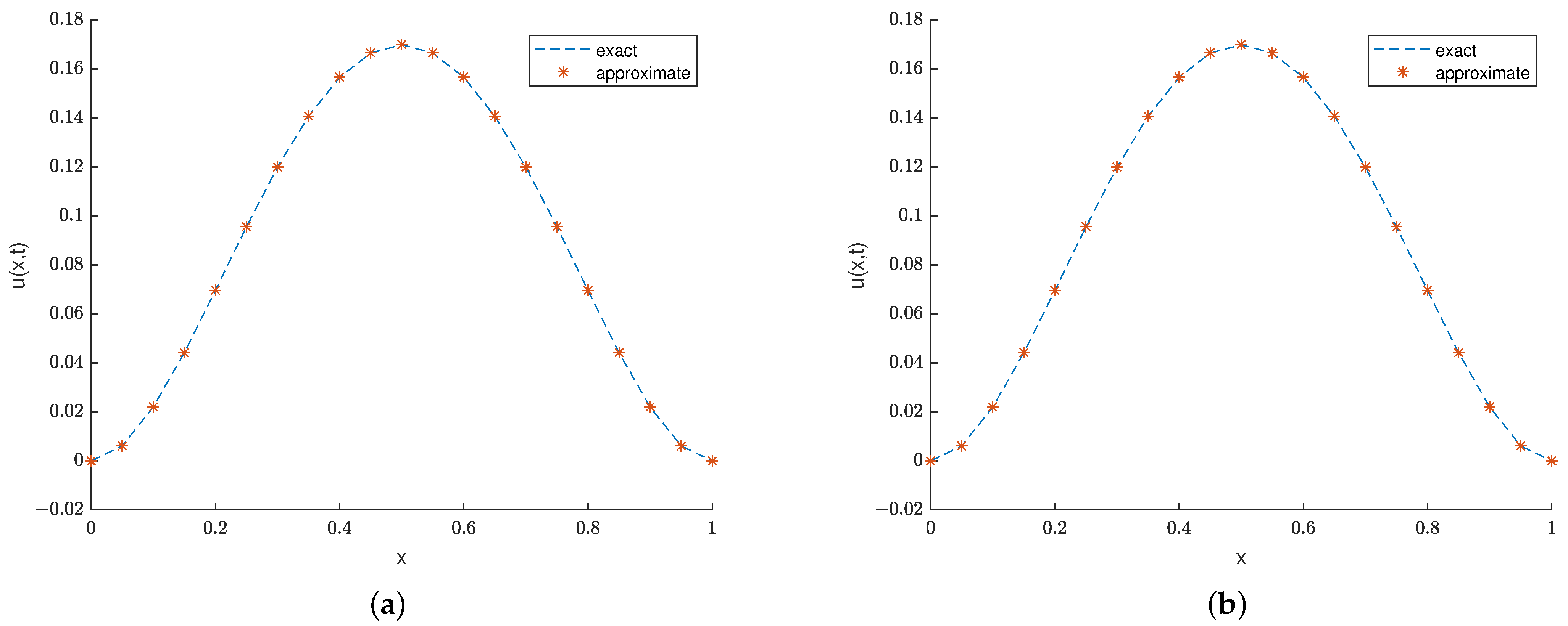
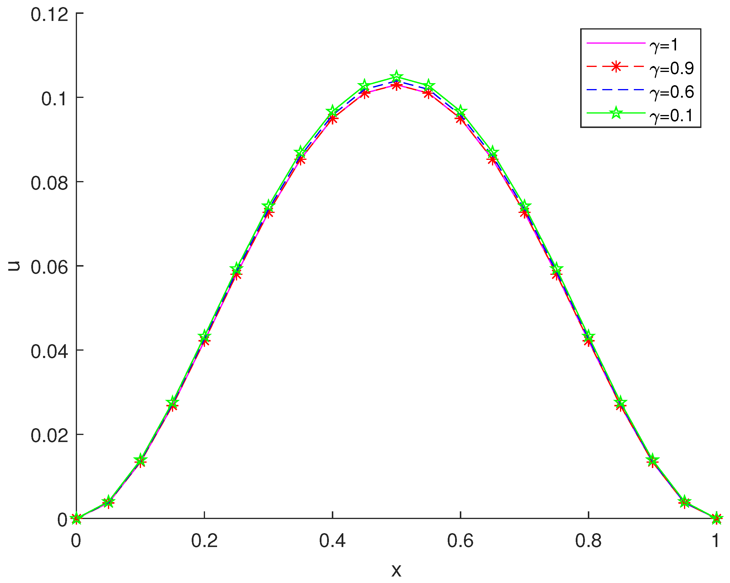
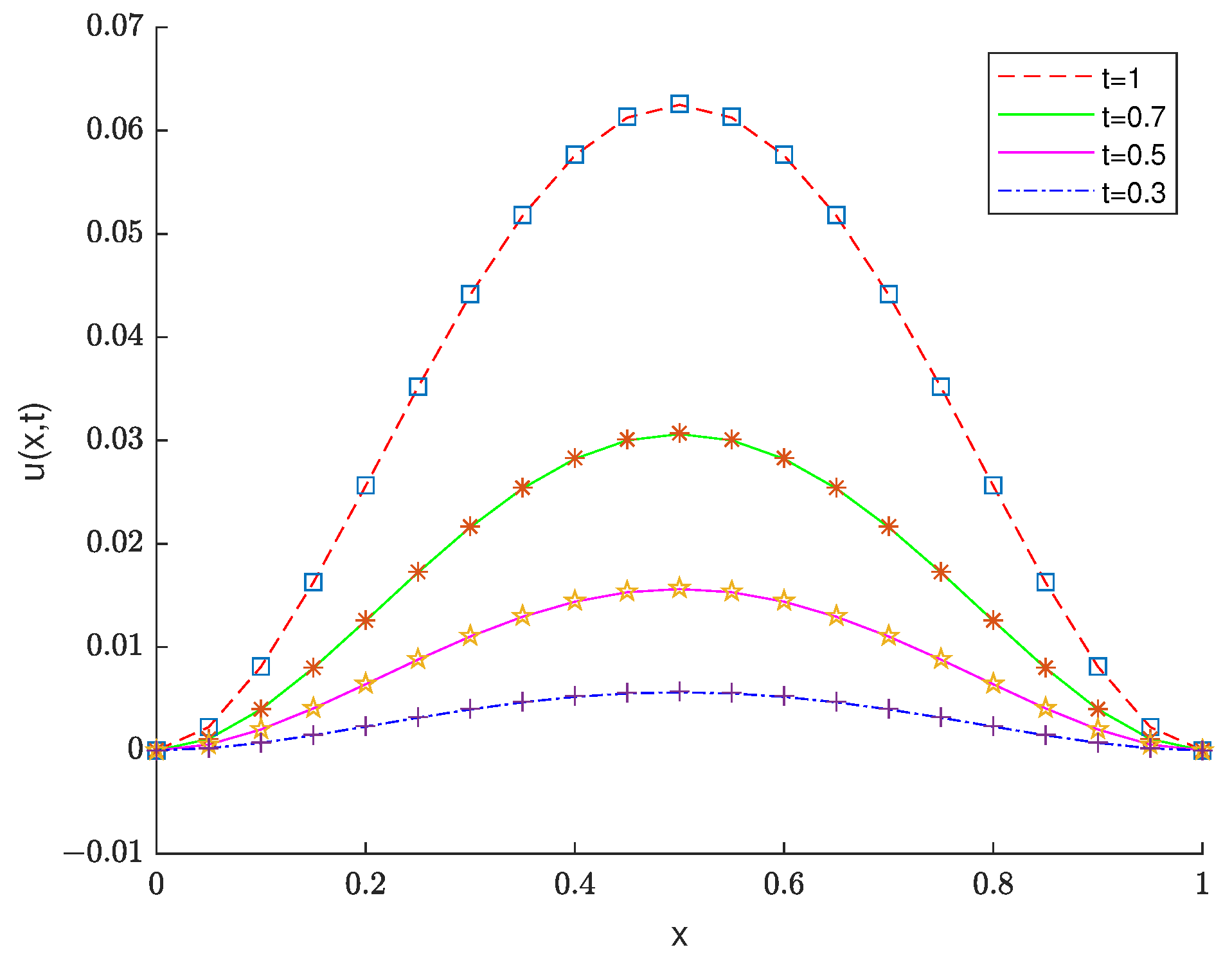
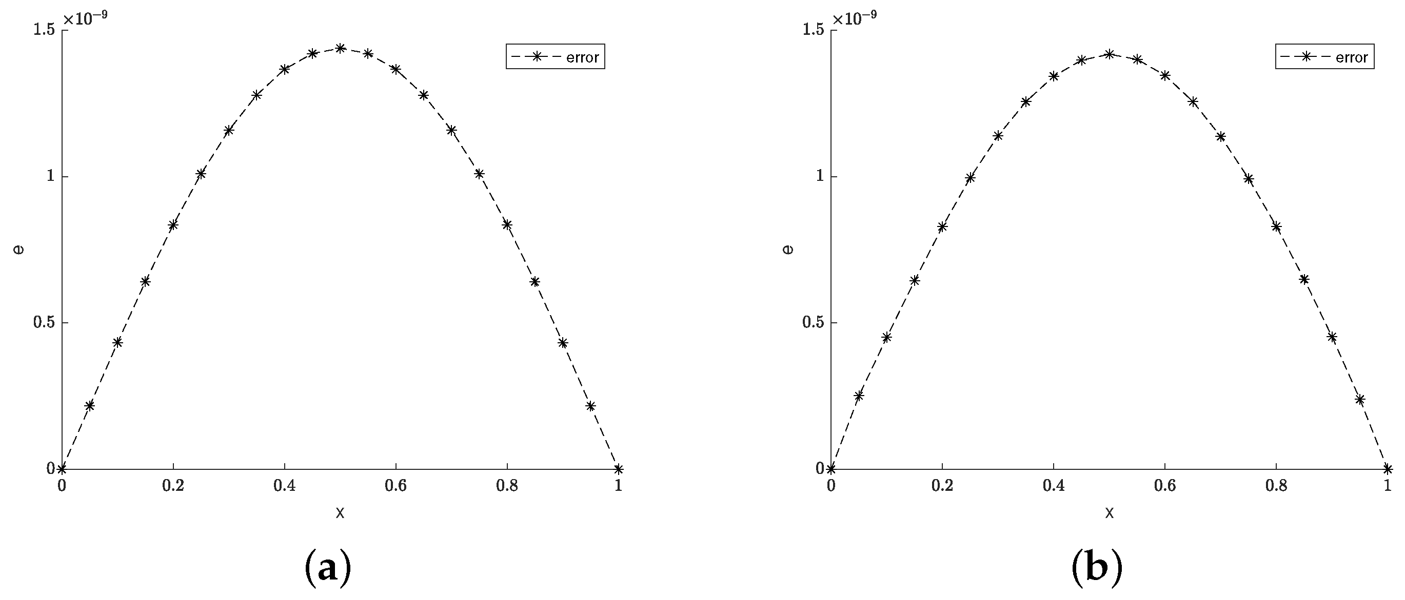
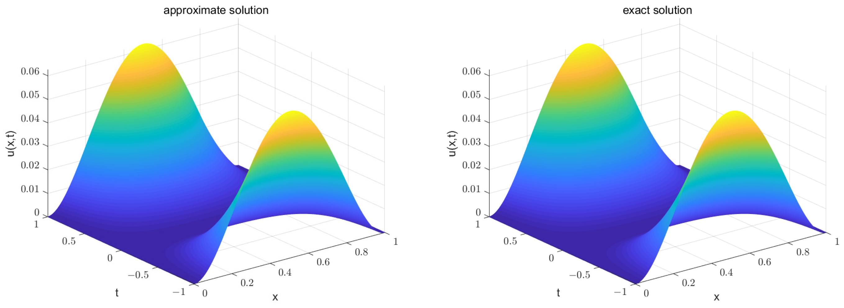
In this section, the stability and convergence of the numerical scheme will be discussed. Assume that $\Omega$ denotes an open bounded region in $R^2$ and let $L_2(\Omega )$ be a Hilbert space with the usual inner product and the norm defined by

$$\parallel u\left(x\right)\parallel =\sqrt{\left(u\right(x),u(x\left)\right)},(u\left(x\right),v\left(x\right))={\int }_{\Omega }u\left(x\right)v\left(x\right)dx.$$

We define

$$H^s(\Omega )=\{u\left(x\right)\in L_2(\Omega ),u^s\left(x\right)\in L_2(\Omega )\}.$$

Lemma 2 

([25]). Suppose $0<s_1<s$ and $u\in H_0^s(\Omega )$, then we have the following fractional Poincare–Friedrichs inequalities

$$C_1\parallel u\parallel \le \parallel {}_0{}^{R}D_x^{s_1}u\parallel \le C_4\parallel {}_0{}^{R}D_x^{s}u\parallel ,$$

where $C_1,C_4$ are positive constants independent of u.

Lemma 3 

([25]). For any $u\in H_0^s(\Omega ),v\in H_0^{{\displaystyle \frac{s}{2}}}(\Omega )$, we have

$$({}_0{}^{R}D_x^{s}u,v)=({}_0{}^{R}D_x^{{\displaystyle \frac{s}{2}}}u,{}_0{}^{R}D_1^{{\displaystyle \frac{s}{2}}}v),({}_x{}^{R}D_1^{s}u,v)=({}_x{}^{R}D_1^{{\displaystyle \frac{s}{2}}}u,{}_0{}^{R}D_x^{{\displaystyle \frac{s}{2}}}v).$$

Lemma 4 

([25]). For $s>0,u\in C_0^{\infty }(\Omega )$. Then,

$$({}_0{}^{R}D_x^{s}u,{}_x{}^{R}D_1^{s}u)=cos\left(s\pi \right)\parallel {}_{-\infty }D_x^s\tilde{u}{\parallel }_{L^2(\Omega )}^2=cos\left(s\pi \right)\parallel {}_x{}^{R}D_{\infty }^s\tilde{u}{\parallel }_{L^2(\Omega )}^2,$$

where $\tilde{u}$ is the extension of u by zero outside Ω. ${}_{-\infty }D_x^s$ denotes a Riemann–Liouville fractional derivative.

Lemma 5 

([21]). For $u^0,u^1,\dots ,u^{k+1}\in H_0^s(\Omega )$, we have

$${\displaystyle \sum _{j=0}^k}{c}_j^{k,\gamma ,\sigma }(u^{k+1-j}-u^{k-j},u^{k+\sigma })\ge {\displaystyle \frac{1}{2}}{\displaystyle \sum _{j=0}^k}{c}_j^{k,\gamma ,\sigma }(\parallel u^{k+1-j}{\parallel }^2-\parallel u^{k-j}{\parallel }^2).$$

Theorem 4. 

Let $u_0\in L_{\infty }(-\mu ,0;H^s),s>0$ and $U^j=u(0,t_j),j=-K,-K+1,\dots ,0,$ then the numerical scheme in Equation (21) is unconditionally stable, i.e.,

$$\parallel U^{k+1}{\parallel }^2\le C^{*}(\parallel U^0{\parallel }^2+C_5),$$

where $C^{*}$ is a constant independent of u and f, $C_5$ is a constant depending on the function f.

Proof. 

Since $u_0\in L_{\infty }(-\mu ,0;H^s)$, thus there exists a constant C such that

$$\parallel U^j{\parallel }^2\le C,j=-K,-K+1,\dots ,0.$$

For $j=1$, multiply v on both sides of the Equation (21) and integrate over the region; we can rewrite Equation (21) in the following form,

$$\begin{array}{cc}\hfill {\displaystyle \frac{{\tau }^{-\gamma }}{\Gamma (2-\gamma )}}(c_0{U}^1-c_0{U}^0,v)& ={\displaystyle \frac{1}{2}}{\displaystyle \sum _{m=0}^{M_1}}{\omega }_m^{(1)}{P}_1({\alpha }_m)({\displaystyle \frac{{\partial }^{{\alpha }_m}{U}^{\sigma }}{{\partial \left|x\right|}^{{\alpha }_m}}},v)+{\displaystyle \frac{1}{2}}{\displaystyle \sum _{m=0}^{M_2}}{\omega }_m^{(2)}{P}_2({\beta }_m)({\displaystyle \frac{{\partial }^{{\beta }_m}{U}^{\sigma }}{{\partial \left|x\right|}^{{\beta }_m}}},v)\hfill \\ \hfill & +(f^{\sigma },v)+r\sigma (U^{1-K},v)+r(1-\sigma )(U^{-K},v).\hfill \end{array}$$

(26)

Taking $v=U^{\sigma }$, from Lemmas 3 and 4, we obtain that

$$\begin{array}{cc}\hfill {\displaystyle \frac{1}{2}}{\displaystyle \sum _{m=0}^{M_1}}{\omega }_m^{(1)}{P}_1({\alpha }_m)({\displaystyle \frac{{\partial }^{{\alpha }_m}{U}^{\sigma }}{{\partial \left|x\right|}^{{\alpha }_m}}},U^{\sigma })& ={\displaystyle \frac{1}{2}}{\displaystyle \sum _{m=0}^{M_1}}{\omega }_m^{(1)}{P}_1({\alpha }_m)(c_{{\alpha }_m}({}_{0}D_x^{{\alpha }_m}{U}^{\sigma },U^{\sigma })+c_{{\alpha }_m}({}_{x}D_1^{{\alpha }_m}{U}^{\sigma },U^{\sigma }))\hfill \\ \hfill & ={\displaystyle \sum _{m=0}^{M_1}}{\omega }_m^{(1)}{P}_1({\alpha }_m){\displaystyle \frac{c_{{\alpha }_m}}{2}}cos({\displaystyle \frac{\pi {\alpha }_m}{2}})(\parallel {}_{0}D_x^{{\displaystyle \frac{{\alpha }_m}{2}}}{U}^{\sigma }{\parallel }^2+\parallel {}_{0}D_x^{{\displaystyle \frac{{\alpha }_m}{2}}}{U}^{\sigma }{\parallel }^2)\hfill \\ \hfill & =-{\displaystyle \frac{1}{2}}{\displaystyle \sum _{m=0}^{M_1}}{\omega }_m^{(1)}{P}_1({\alpha }_m){\parallel {}_{0}D_x^{{\displaystyle \frac{{\alpha }_m}{2}}}{U}^{\sigma }\parallel }^2,\hfill \end{array}$$

(27)

$$\begin{array}{cc}\hfill {\displaystyle \frac{1}{2}}{\displaystyle \sum _{m=0}^{M_2}}{\omega }_m^{(2)}{P}_2({\beta }_m)({\displaystyle \frac{{\partial }^{{\beta }_m}{U}^{\sigma }}{{\partial \left|x\right|}^{{\beta }_m}}},U^{\sigma })& ={\displaystyle \frac{1}{2}}{\displaystyle \sum _{m=0}^{M_2}}{\omega }_m^{(2)}{P}_2({\beta }_m)(c_{{\beta }_m}({}_{0}D_x^{{\beta }_m}{U}^{\sigma },U^{\sigma })+c_{{\beta }_m}({}_{x}D_1^{{\beta }_m}{U}^{\sigma },U^{\sigma }))\hfill \\ \hfill & ={\displaystyle \sum _{m=0}^{M_2}}{\omega }_m^{(2)}{P}_2({\beta }_m){\displaystyle \frac{c_{{\beta }_m}}{2}}cos({\displaystyle \frac{\pi {\beta }_m}{2}})(\parallel {}_{0}D_x^{{\displaystyle \frac{{\beta }_m}{2}}}{U}^{\sigma }{\parallel }^2+\parallel {}_{0}D_x^{{\displaystyle \frac{{\beta }_m}{2}}}{U}^{\sigma }{\parallel }^2)\hfill \\ \hfill & =-{\displaystyle \frac{1}{2}}{\displaystyle \sum _{m=0}^{M_2}}{\omega }_m^{(2)}{P}_2({\beta }_m){\parallel {}_{0}D_x^{{\displaystyle \frac{{\beta }_m}{2}}}{U}^{\sigma }\parallel }^2.\hfill \end{array}$$

(28)

By Lemma 2, we have

$${\displaystyle \sum _{m=0}^{M_1}}{\omega }_m^{(1)}{P}_1({\alpha }_m)\parallel {}_{0}D_x^{{\displaystyle \frac{{\alpha }_m}{2}}}{U}^{\sigma }{\parallel }^2+{\displaystyle \sum _{m=0}^{M_2}}{\omega }_m^{(2)}{P}_2({\beta }_m)\parallel {}_{0}D_x^{{\displaystyle \frac{{\beta }_m}{2}}}{U}^{\sigma }{\parallel }^2\ge C_2{\parallel U^{\sigma }\parallel }^2.$$

(29)

Using Young’s inequality, we obtain

$$(f^{\sigma },U^{\sigma })\le {\displaystyle \frac{1}{C_2}}\parallel f^{\sigma }{\parallel }^2+{\displaystyle \frac{C_2}{4}}{\parallel U^{\sigma }\parallel }^2,$$

(30)

$$r(U^{\sigma -K},U^{\sigma })\le {\displaystyle \frac{r^2}{C_2}}\parallel U^{\sigma -K}{\parallel }^2+{\displaystyle \frac{C_2}{4}}{\parallel U^{\sigma }\parallel }^2.$$

(31)

Combining (26)–(31), we have

$$\begin{array}{cc}\hfill & \eta c_0\parallel U^1{\parallel }^2+{\displaystyle \frac{C_2}{2}}{\parallel U^{\sigma }\parallel }^2\hfill \\ \hfill & \le \eta c_0{\parallel U^1\parallel }^2+{\displaystyle \frac{1}{2}}{\displaystyle \sum _{m=0}^{M_1}}{\omega }_m^{(1)}{P}_1({\alpha }_m){\parallel {}_{0}D_x^{{\displaystyle \frac{{\alpha }_m}{2}}}{U}^{\sigma }\parallel }^2+{\displaystyle \frac{1}{2}}{\displaystyle \sum _{m=0}^{M_2}}{\omega }_m^{(2)}{P}_2({\beta }_m){\parallel {}_{0}D_x^{{\displaystyle \frac{{\beta }_m}{2}}}{U}^{\sigma }\parallel }^2\hfill \\ \hfill & \le \eta c_0\parallel U^0{\parallel }^2+{\displaystyle \frac{1}{C_2}}\parallel f^{\sigma }{\parallel }^2+{\displaystyle \frac{C_2}{4}}\parallel U^{\sigma }{\parallel }^2+{\displaystyle \frac{r^2}{C_2}}\parallel U^{\sigma -K}{\parallel }^2+{\displaystyle \frac{C_2}{4}}{\parallel U^{\sigma }\parallel }^2\hfill \\ \hfill & \le \eta c_0\parallel U^0{\parallel }^2+{\displaystyle \frac{1}{C_2}}\parallel f^{\sigma }{\parallel }^2+{\displaystyle \frac{C_2}{2}}\parallel U^{\sigma }{\parallel }^2+{\displaystyle \frac{r^2}{C_2}}{\parallel U^{\sigma -K}\parallel }^2,\hfill \end{array}$$

where $\eta ={\displaystyle \frac{{\tau }^{-\gamma }}{\Gamma (2-\gamma )}}$. Thus, we have

$$\begin{array}{cc}\hfill \parallel U^1{\parallel }^2& \le \parallel U^0{\parallel }^2+{\displaystyle \frac{r_1}{C_2{c}_0\eta }}+{\displaystyle \frac{r^2}{C_2\eta c_0}}\parallel U^{\sigma -K}{\parallel }^2\le {\parallel U^0\parallel }^2+C_3,\hfill \end{array}$$

where $r_1=\underset{0\le l\le n}{max}\parallel f_l^{k+\sigma }\parallel$. Now, we assume that

$$\parallel U^j{\parallel }^2\le C,j=-K,-K+1,\dots ,k.k=1,2,\dots ,K_1-1.$$

Next, we prove $\parallel U^{k+1}\parallel$, multiply v on both sides of Equation (21), and integrate over the region. We can rewrite Equation (21) in the following form:

$$\begin{array}{cc}\hfill & {\displaystyle \frac{{\tau }^{-\gamma }}{\Gamma (2-\gamma )}}({\displaystyle \sum _{j=0}^k}{c}_j(U_{k+1-j}-U_{k-j}),v)\hfill \\ \hfill & ={\displaystyle \frac{1}{2}}{\displaystyle \sum _{m=0}^{M_1}}{\omega }_m^{(1)}{P}_1({\alpha }_m)({\displaystyle \frac{{\partial }^{{\alpha }_m}{U}^{k+\sigma }}{{\partial \left|x\right|}^{{\alpha }_m}}},v)+{\displaystyle \frac{1}{2}}{\displaystyle \sum _{m=0}^{M_2}}{\omega }_m^{(2)}{P}_2({\beta }_m)({\displaystyle \frac{{\partial }^{{\beta }_m}{U}^{k+\sigma }}{{\partial \left|x\right|}^{{\beta }_m}}},v)\hfill \\ \hfill & +(f^{k+\sigma },v)+r\sigma (U^{k+1-K},v)+r(1-\sigma )(U^{k-K},v).\hfill \end{array}$$

(32)

Taking $v=U^{k+\sigma }$, we have

$$\begin{array}{cc}\hfill & {\displaystyle \frac{1}{2}}{\displaystyle \sum _{m=0}^{M_1}}{\omega }_m^{(1)}{P}_1({\alpha }_m)({\displaystyle \frac{{\partial }^{{\alpha }_m}{U}^{k+\sigma }}{{\partial \left|x\right|}^{{\alpha }_m}}},U^{k+\sigma })={\displaystyle \frac{1}{2}}{\displaystyle \sum _{m=0}^{M_1}}{\omega }_m^{(1)}{P}_1({\alpha }_m)c_{{\alpha }_m}({}_{0}D_x^{{\alpha }_m}{U}^{k+\sigma }+{}_{x}D_1^{{\alpha }_m}{U}^{k+\sigma },U^{k+\sigma })\hfill \\ \hfill & ={\displaystyle \frac{1}{2}}{\displaystyle \sum _{m=0}^{M_1}}{\omega }_m^{(1)}{P}_1({\alpha }_m)c_{{\alpha }_m}cos({\displaystyle \frac{\pi {\alpha }_m}{2}})(\parallel {}_{0}D_x^{{\displaystyle \frac{{\alpha }_m}{2}}}{U}^{k+\sigma }{\parallel }^2+\parallel {}_{0}D_x^{{\displaystyle \frac{{\alpha }_m}{2}}}{U}^{k+\sigma }{\parallel }^2)\hfill \\ \hfill & =-{\displaystyle \frac{1}{2}}{\displaystyle \sum _{m=0}^{M_1}}{\omega }_m^{(1)}{P}_1({\alpha }_m){\parallel {}_{0}D_x^{{\displaystyle \frac{{\alpha }_m}{2}}}{U}^{k+\sigma }\parallel }^2,\hfill \end{array}$$

(33)

$$\begin{array}{cc}\hfill & {\displaystyle \frac{1}{2}}{\displaystyle \sum _{m=0}^{M_2}}{\omega }_m^{(2)}{P}_2({\beta }_m)({\displaystyle \frac{{\partial }^{{\beta }_m}{U}^{k+\sigma }}{{\partial \left|x\right|}^{{\beta }_m}}},U^{k+\sigma })={\displaystyle \frac{1}{2}}{\displaystyle \sum _{m=0}^{M_2}}{\omega }_m^{(2)}{P}_2({\beta }_m)c_{{\beta }_m}({}_{0}D_x^{{\beta }_m}{U}^{k+\sigma }+{}_{x}D_1^{{\beta }_m}{U}^{k+\sigma },U^{k+\sigma }))\hfill \\ \hfill & ={\displaystyle \frac{1}{2}}{\displaystyle \sum _{m=0}^{M_2}}{\omega }_m^{(2)}{P}_2({\beta }_m)c_{{\beta }_m}cos({\displaystyle \frac{\pi {\beta }_m}{2}})(\parallel {}_{0}D_x^{{\displaystyle \frac{{\beta }_m}{2}}}{U}^{k+\sigma }{\parallel }^2+{}_{0}D_x^{{\displaystyle \frac{{\beta }_m}{2}}}{U}^{k+\sigma }{\parallel }^2)\hfill \\ \hfill & =-{\displaystyle \frac{1}{2}}{\displaystyle \sum _{m=0}^{M_2}}{\omega }_m^{(2)}{P}_2({\beta }_m){\parallel {}_{0}D_x^{{\displaystyle \frac{{\beta }_m}{2}}}{U}^{k+\sigma }\parallel }^2.\hfill \end{array}$$

(34)

Using Lemma 2, we obtain that

$${\displaystyle \sum _{m=0}^{M_1}}{\omega }_m^{(1)}{P}_1({\alpha }_m)\parallel {}_{0}D_x^{{\displaystyle \frac{{\alpha }_m}{2}}}{U}^{k+\sigma }{\parallel }^2+{\displaystyle \sum _{m=0}^{M_2}}{\omega }_m^{(2)}{P}_2({\beta }_m)\parallel {}_{0}D_x^{{\displaystyle \frac{{\beta }_m}{2}}}{U}^{k+\sigma }{\parallel }^2\ge C_2{\parallel U^{k+\sigma }\parallel }^2.$$

(35)

From Lemma 5, we have

$${\displaystyle \frac{{\tau }^{-\gamma }}{\Gamma (2-\gamma )}}{\displaystyle \sum _{j=0}^k}{c}_j^{(k,\gamma ,\sigma )}(U^{k+1-j}-U^{k-j},U^{k+\sigma })\ge {\displaystyle \frac{1}{2}}{\displaystyle \frac{{\tau }^{-\gamma }}{\Gamma (2-\gamma )}}{\displaystyle \sum _{j=0}^k}{c}_j^{(k,\gamma ,\sigma )}(\parallel U^{k+1-j}{\parallel }^2-\parallel U^{k-j}{\parallel }^2).$$

(36)

Then, combining (32)–(36) and Young’s inequality, we obtain

$$\begin{array}{cc}\hfill & {\displaystyle \frac{\eta c_0}{2}}\parallel U^{k+1}{\parallel }^2+{\displaystyle \frac{C_2}{2}}{\parallel U^{k+\sigma }\parallel }^2\hfill \\ \hfill & \le {\displaystyle \frac{\eta c_0}{2}}\parallel U^{k+1}{\parallel }^2+{\displaystyle \frac{1}{2}}{\displaystyle \sum _{m=0}^{M_1}}{\omega }_m^{(1)}{P}_1({\alpha }_m){\parallel {}_{0}D_x^{{\displaystyle \frac{{\alpha }_m}{2}}}{U}^{k+\sigma }\parallel }^2+{\displaystyle \frac{1}{2}}{\displaystyle \sum _{m=0}^{M_2}}{\omega }_m^{(2)}{P}_2({\beta }_m){\parallel {}_{0}D_x^{{\beta }_m}{U}^{k+\sigma }\parallel }^2\hfill \\ \hfill & \le {\displaystyle \frac{\eta }{2}}{\displaystyle \sum _{j=1}^k}(c_{k+1-j}-c_{k-j})\parallel U^j{\parallel }^2+{\displaystyle \frac{\eta c_k}{2}}\parallel U^0{\parallel }^2+{\displaystyle \frac{1}{C_2}}\parallel f^{k+\sigma }{\parallel }^2+{\displaystyle \frac{r^2}{C_2}}\parallel U^{k+\sigma -K}{\parallel }^2+{\displaystyle \frac{C_2}{2}}{\parallel U^{k+\sigma }\parallel }^2.\hfill \end{array}$$

By Gronwall’s inequality, we have

$$\begin{array}{cc}\hfill \parallel U^{k+1}{\parallel }^2& \le exp({\displaystyle \frac{1}{c_0}}{\displaystyle \sum _{j=1}^k}(c_{k+1-j}-c_{k-j}))(\parallel U^0{\parallel }^2+{\displaystyle \frac{2}{c_0\eta C_2}}\parallel f^{k+\sigma }{\parallel }^2+{\displaystyle \frac{2r^2}{\eta c_0{C}_2}}\parallel U^{k+\sigma -K}{\parallel }^2)\hfill \\ \hfill & \le e(\parallel U^0{\parallel }^2+{\displaystyle \frac{2r_1}{c_0\eta C_2}}+{\displaystyle \frac{2r^2}{\eta c_0{C}_2}}C)\le C^{*}(\parallel U^0{\parallel }^2+C_5),\hfill \end{array}$$

where $r_1=\underset{0\le l\le n}{max}\parallel f_l^{k+\sigma }\parallel$, which completes the proof. □

Theorem 5. 

Let $\tilde{u}$ be the exact solution of Equation (1) and ${\left\{u^k\right\}}_{k=0}^{K_1+1}$ be the time-discrete solution of (21), then we have the following error estimates:

$$\begin{array}{c}\hfill \parallel e^{k+1}\parallel \le C(M^{-r_1}+{\tau }^2),k=0,\dots ,K_1-1,\end{array}$$

where C is a constant.

Proof. 

Let $e^k=\tilde{u}(x_p,t_k)-u(x_p,t_k)$, with the error equation:

$$\begin{array}{cc}\hfill & {\displaystyle \frac{{\tau }^{-\alpha }}{\Gamma (2-\alpha )}}(c_0{e}^{k+1}-{\displaystyle \sum _{j=1}^k}(c_{k+1-j}-c_{k-j})e^j-c_k{e}^0)\hfill \\ \hfill & ={\displaystyle \frac{1}{2}}{\displaystyle \sum _{m=0}^{M_1}}{\omega }_m^{(1)}{P}_1({\alpha }_m){\displaystyle \frac{{\partial }^{{\alpha }_m}{e}^{k+\sigma }}{{\partial \left|x\right|}^{{\alpha }_m}}}+{\displaystyle \frac{1}{2}}{\displaystyle \sum _{m=0}^{M_2}}{\omega }_m^{(2)}{P}_2({\beta }_m){\displaystyle \frac{{\partial }^{{\beta }_m}{e}^{k+\sigma }}{{\partial \left|x\right|}^{{\beta }_m}}}+r{e}^{k+\sigma -K}+O(M^{-r_1})+O({\tau }^2).\hfill \end{array}$$

(37)

Combining the proof process of Theorem 4, we have

$$\begin{array}{cc}\hfill \parallel e^{k+1}{\parallel }^2& \le e(\parallel e^0{\parallel }^2+{\displaystyle \frac{2r^2}{\eta c_0{C}_2}}\parallel e^{k+\sigma -K}{\parallel }^2+{\displaystyle \frac{4}{c_0\eta C_2}}O(M^{-2r_1})+{\displaystyle \frac{4}{c_0\eta C_2}}O({\tau }^4)).\hfill \end{array}$$

Thus,

$$\begin{array}{c}\hfill \parallel e^{k+1}\parallel \le C(M^{-r_1}+{\tau }^2)\end{array},$$

where $M=max(M_h),h=1,2.$ The proof is completed. □

6. Test Examples

In this paper, the above numerical methods are used to carry out specific numerical calculations, and examples are given to illustrate the effectiveness, accuracy, and precision of the constructed numerical methods in solving a time-fractional and Riesz space distributed-order advection–diffusion equation with time-delay.

Example 1. 

We consider the following time-fractional and Riesz space distributed-order advection–diffusion equation with time-delay

$${}_0{}^{C}D_t^{\gamma }u(x,t)={\int }_1^2{P}_1(\alpha ){\displaystyle \frac{{\partial }^{\alpha }u(x,t)}{{\partial \left|x\right|}^{\alpha }}}d\alpha +{\int }_0^1{P}_2(\beta ){\displaystyle \frac{{\partial }^{\beta }u(x,t)}{{\partial \left|x\right|}^{\beta }}}d\beta +ru(x,t-1)+f(x,t),$$

(38)

with initial and boundary conditions

$$u(x,t)=x^2{(1-x)}^2{e}^t,-1\le t\le 0,0\le x\le 1,$$

(39)

$$u(0,t)=u(1,t)=0,0\le t\le T,$$

(40)

where

$$P_1(\alpha )=-2\Gamma (5-\alpha )cos(\alpha \pi /2),1<\alpha \le 2,$$

$$P_2(\beta )=\left\{\begin{array}{cc}0,\hfill & 0<\beta \le 1/2,\hfill \\ 2\Gamma (5-\beta )cos(\beta \pi /2),\hfill & {\displaystyle \frac{1}{2}}<\beta \le 1,\hfill \end{array}\right.$$

and $f(x,t)=e^t{x}^2{(1-x)}^2-e^{t-1}{x}^2{(1-x)}^2-r{e}^t[R_1(x)+R_1(1-x)-R_2(x)-R_2(1-x)],$ where

$$\begin{array}{cc}\hfill R_1(x)& =\Gamma (5){\displaystyle \frac{(x^3-x^2)}{ln(x)}}-2\Gamma (4)\left[{\displaystyle \frac{(3x^2-2x)}{ln(x)}}-{\displaystyle \frac{x^2-x}{{(ln(x))}^2}}\right]\hfill \\ \hfill & +{\displaystyle \frac{\Gamma (3)}{ln(x)}}\left[6x-2-{\displaystyle \frac{5x}{ln(x)}}+{\displaystyle \frac{3}{ln(x)}}+{\displaystyle \frac{2x}{{(ln(x))}^2}}-{\displaystyle \frac{2}{{(ln(x))}^2}}\right]\hfill \end{array},$$

$$\begin{array}{cc}\hfill R_2(x)& =\Gamma (5){\displaystyle \frac{(x^{\frac{7}{2}}-x^3)}{ln(x)}}-2\Gamma (4)\left[{\displaystyle \frac{(\frac{7}{2}{x}^{\frac{5}{2}}-3x^2)}{ln(x)}}-{\displaystyle \frac{(x^{\frac{5}{2}}-x^2)}{{(ln(x))}^2}}\right]\hfill \\ \hfill & +{\displaystyle \frac{\Gamma (3)}{ln(x)}}\left[{\displaystyle \frac{35}{4}}{x}^{{\displaystyle \frac{3}{2}}}-6x-{\displaystyle \frac{6x^{\frac{3}{2}}}{ln(x)}}+{\displaystyle \frac{5x}{ln(x)}}+{\displaystyle \frac{2x^{\frac{3}{2}}}{{(ln(x))}^2}}-{\displaystyle \frac{2x}{{(ln(x))}^2}}\right]\hfill \end{array}.$$

The exact solution of this problem is $u(x,t)=x^2{(1-x)}^2{e}^t$ in the case of $\gamma =1$.

When $n=3$, we have

$$\begin{array}{cc}\hfill & \eta (c_0{\displaystyle \sum _{i=0}^3}{\lambda }_i^{k+1}{T}_i^{*}(x_p)-{\displaystyle \sum _{j=1}^k}{\displaystyle \sum _{i=0}^3}(c_{k-j}-c_{k-j-1}){\lambda }_i^j{T}_i^{*}(x_p)-c_k{\displaystyle \sum _{i=0}^3}{\lambda }_i^0{T}_i^{*}(x_p))\hfill \\ \hfill & ={\displaystyle \sum _{m=0}^{M_1}}{P}_1({\alpha }_m)w_m^1{c}_{{\alpha }_m}({\displaystyle \sum _{i=0}^3}{\displaystyle \sum _{l=0}^i}{\lambda }_i^{k+\sigma }({\gamma }_{i,l}^{{\alpha }_m}{x}_p^{i-l-{\alpha }_m}+{\gamma }_{i,l}^{{\alpha }_m}{(1-x_p)}^{i-l-{\alpha }_m}))\hfill \\ \hfill & +{\displaystyle \sum _{m=0}^{M_2}}{P}_2({\beta }_m)w_m^2{c}_{{\beta }_m}({\displaystyle \sum _{i=0}^3}{\displaystyle \sum _{l=0}^i}{\lambda }_i^{k+\sigma }({\gamma }_{i,l}^{{\beta }_m}{x}_p^{i-l-{\beta }_m}+{\gamma }_{i,l}^{{\beta }_m}{(1-x_p)}^{i-l-{\beta }_m}))\hfill \\ \hfill & +\tau f^{k+\sigma }+r\sigma {\displaystyle \sum _{i=0}^3}{\lambda }_i^{k+1-K}{T}_i^{*}(x_p)+r(1-\sigma ){\displaystyle \sum _{i=0}^3}{\lambda }_i^{k-K}{T}_i^{*}(x_p),\hfill \end{array}$$

(41)

$$p=1,2.k=0,1,\dots ,K_1-1.$$

$${\displaystyle \sum _{i=0}^3}{(-1)}^{i+2}(i+1){\lambda }_i(0)=0,$$

(42)

$${\displaystyle \sum _{i=0}^3}(i+1){\lambda }_i(1)=0.$$

(43)

Then, consdering Equations (41)–(43) comprehensively, and expressing them in the following matrix form:

$$\begin{array}{cc}\hfill & (A-\sigma {\displaystyle \sum _{m=0}^{M_1}}{P}_1({\alpha }_m){\omega }_m^1{c}_{{\alpha }_m}(C_1+C_2)-\sigma {\displaystyle \sum _{m=0}^{M_2}}{P}_2({\beta }_m){\omega }_m^2{c}_{{\beta }_m}(D_1+D_2))U^{k+1}\hfill \\ \hfill & =\eta {\displaystyle \sum _{j=1}^k}(c_{k+1-j}-c_{k-j})B{U}^j+\eta c_{k}B{U}^0+((1-\sigma ){\displaystyle \sum _{m=0}^{M_1}}{P}_1({\alpha }_m){\omega }_m^1{c}_{{\alpha }_m}(C_1+C_2)+(1-\sigma )F_2\hfill \\ \hfill & +(1-\sigma ){\displaystyle \sum _{m=0}^{M_2}}{P}_2({\beta }_m){\omega }_m^2{c}_{{\beta }_m}(D_1+D_2))U^k+\sigma F_1+r\sigma B{U}^{k+1-K}+r(1-\sigma )B{U}^{k-K},\hfill \end{array}$$

where

$$A=\left(\begin{array}{cccc}\eta c_0{T}_0^{*}(x_1)& \eta c_0{T}_1^{*}(x_1)& \eta c_0{T}_2^{*}(x_1)& \eta c_0{T}_3^{*}(x_1)\\ \eta c_0{T}_0^{*}(x_2)& \eta c_0{T}_1^{*}(x_2)& \eta c_0{T}_2^{*}(x_2)& \eta c_0{T}_3^{*}(x_2)\\ 1& -2& 3& -4\\ 1& 2& 3& 4\end{array}\right),C_1=\left(\begin{array}{cccc}{c}_{11}& c_{12}& c_{13}& c_{14}\\ c_{21}& c_{22}& c_{23}& c_{24}\\ 0& 0& 0& 0\\ 0& 0& 0& 0\end{array}\right),$$

$$B=\left(\begin{array}{cccc}{T}_0^{*}(x_1)& T_1^{*}(x_1)& T_2^{*}(x_1)& T_3^{*}(x_1)\\ T_0^{*}(x_2)& T_1^{*}(x_2)& T_2^{*}(x_2)& T_3^{*}(x_2)\\ 0& 0& 0& 0\\ 0& 0& 0& 0\end{array}\right),C_2=\left(\begin{array}{cccc}{\tilde{c}}_{11}& {\tilde{c}}_{12}& {\tilde{c}}_{13}& {\tilde{c}}_{14}\\ {\tilde{c}}_{21}& {\tilde{c}}_{22}& {\tilde{c}}_{23}& {\tilde{c}}_{24}\\ 0& 0& 0& 0\\ 0& 0& 0& 0\end{array}\right),F_2=\left(\begin{array}{c}{f}_1^k\\ f_2^k\\ 0\\ 0\end{array}\right),$$

$$D_1=\left(\begin{array}{cccc}{d}_{11}& d_{12}& d_{13}& d_{14}\\ d_{21}& d_{22}& d_{23}& d_{24}\\ 0& 0& 0& 0\\ 0& 0& 0& 0\end{array}\right),D_2=\left(\begin{array}{cccc}{\tilde{d}}_{11}& {\tilde{d}}_{12}& {\tilde{d}}_{13}& {\tilde{d}}_{14}\\ {\tilde{d}}_{21}& {\tilde{d}}_{22}& {\tilde{d}}_{23}& {\tilde{d}}_{24}\\ 0& 0& 0& 0\\ 0& 0& 0& 0\end{array}\right),F_1=\left(\begin{array}{c}{f}_1^{k+1}\\ f_2^{k+1}\\ 0\\ 0\end{array}\right),$$

$$c_{11}={\gamma }_{0,0}^{\alpha }{x}_1^{-\alpha },c_{12}={\gamma }_{1,0}^{\alpha }{x}_1^{1-\alpha }+{\gamma }_{1,1}^{\alpha }{x}_1^{-\alpha },c_{13}={\gamma }_{2,0}^{\alpha }{x}_1^{2-\alpha }+{\gamma }_{2,1}^{\alpha }{x}_1^{1-\alpha }+{\gamma }_{2,2}^{\alpha }{x}_1^{-\alpha },$$

$$c_{14}={\gamma }_{2,0}^{\alpha }{x}_1^{2-\alpha }+{\gamma }_{2,1}^{\alpha }{x}_1^{1-\alpha }+{\gamma }_{2,2}^{\alpha }{x}_1^{-\alpha },c_{21}={\gamma }_{0,0}^{\alpha }{x}_2^{-\alpha },c_{22}={\gamma }_{1,0}^{\alpha }{x}_2^{1-\alpha }+{\gamma }_{1,1}^{\alpha }{x}_2^{-\alpha },$$

$$c_{23}={\gamma }_{2,0}^{\alpha }{x}_2^{2-\alpha }+{\gamma }_{2,1}^{\alpha }{x}_2^{1-\alpha }+{\gamma }_{2,2}^{\alpha }{x}_2^{-\alpha },c_{24}={\gamma }_{3,0}^{\alpha }{x}_2^{3-\alpha }+{\gamma }_{3,1}^{\alpha }{x}_2^{2-\alpha }+{\gamma }_{3,2}^{\alpha }{x}_2^{1-\alpha }+{\gamma }_{3,3}^{\alpha }{x}_2^{-\alpha },$$

$${\tilde{c}}_{11}={\gamma }_{0,0}^{\alpha }{(1-x_1)}^{-\alpha },{\tilde{c}}_{12}={\gamma }_{1,0}^{\alpha }{(1-x_1)}^{1-\alpha }+{\gamma }_{1,1}^{\alpha }{(1-x_1)}^{-\alpha },$$

$${\tilde{c}}_{13}={\gamma }_{2,0}^{\alpha }{(1-x_1)}^{2-\alpha }+{\gamma }_{2,1}^{\alpha }{(1-x_1)}^{1-\alpha }+{\gamma }_{2,2}^{\alpha }{(1-x_1)}^{-\alpha },$$

$$c_{14}={\gamma }_{2,0}^{\alpha }{(1-x_1)}^{2-\alpha }+{\gamma }_{2,1}^{\alpha }{(1-x_1)}^{1-\alpha }+{\gamma }_{2,2}^{\alpha }{(1-x_1)}^{-\alpha },{\tilde{c}}_{21}={\gamma }_{0,0}^{\alpha }{(1-x_2)}^{-\alpha },$$

$${\tilde{c}}_{22}={\gamma }_{1,0}^{\alpha }{(1-x_2)}^{1-\alpha }+{\gamma }_{1,1}^{\alpha }{(1-x_2)}^{-\alpha },{\tilde{c}}_{23}={\gamma }_{2,0}^{\alpha }{(1-x_2)}^{2-\alpha }+{\gamma }_{2,1}^{\alpha }{(1-x_2)}^{1-\alpha }+{\gamma }_{2,2}^{\alpha }{(1-x_2)}^{-\alpha },$$

$${\tilde{c}}_{24}={\gamma }_{3,0}^{\alpha }{(1-x_2)}^{3-\alpha }+{\gamma }_{3,1}^{\alpha }{(1-x_2)}^{2-\alpha }+{\gamma }_{3,2}^{\alpha }{(1-x_2)}^{1-\alpha }+{\gamma }_{3,3}^{\alpha }{(1-x_2)}^{-\alpha },$$

$$d_{11}={\gamma }_{0,0}^{\beta }{x}_1^{-\beta },d_{12}={\gamma }_{1,0}^{\beta }{x}_1^{1-\beta }+{\gamma }_{1,1}^{\beta }{x}_1^{-\beta },d_{13}={\gamma }_{2,0}^{\beta }{x}_1^{2-\beta }+{\gamma }_{2,1}^{\beta }{x}_1^{1-\beta }+{\gamma }_{2,2}^{\beta }{x}_1^{-\beta },$$

$$d_{14}={\gamma }_{2,0}^{\beta }{x}_1^{2-\beta }+{\gamma }_{2,1}^{\beta }{x}_1^{1-\beta }+{\gamma }_{2,2}^{\beta }{x}_1^{-\beta },d_{21}={\gamma }_{0,0}^{\beta }{x}_2^{-\beta }{d}_{22}={\gamma }_{1,0}^{\beta }{x}_2^{1-\beta }+{\gamma }_{1,1}^{\beta }{x}_2^{-\beta },$$

$$d_{23}={\gamma }_{2,0}^{\beta }{x}_2^{2-\beta }+{\gamma }_{2,1}^{\beta }{x}_2^{1-\beta }+{\gamma }_{2,2}^{\beta }{x}_2^{-\beta },d_{24}={\gamma }_{3,0}^{\beta }{x}_2^{3-\beta }+{\gamma }_{3,1}^{\beta }{x}_2^{2-\beta }+{\gamma }_{3,2}^{\beta }{x}_2^{1-\beta }+{\gamma }_{3,3}^{\beta }{x}_2^{-\beta },$$

$${\tilde{d}}_{11}={\gamma }_{0,0}^{\beta }{(1-x_1)}^{-\beta },{\tilde{d}}_{12}={\gamma }_{1,0}^{\beta }{(1-x_1)}^{1-\beta }+{\gamma }_{1,1}^{\beta }{(1-x_1)}^{-\beta },$$

$${\tilde{d}}_{13}={\gamma }_{2,0}^{\beta }{(1-x_1)}^{2-\beta }+{\gamma }_{2,1}^{\beta }{(1-x_1)}^{1-\beta }+{\gamma }_{2,2}^{\beta }{(1-x_1)}^{-\beta },$$

$${\tilde{d}}_{14}={\gamma }_{2,0}^{\beta }{(1-x_1)}^{2-\beta }+{\gamma }_{2,1}^{\beta }{(1-x_1)}^{1-\beta }+{\gamma }_{2,2}^{\beta }{(1-x_1)}^{-\beta },{\tilde{d}}_{21}={\gamma }_{0,0}^{\beta }{(1-x_2)}^{-\beta },$$

$${\tilde{d}}_{22}={\gamma }_{1,0}^{\beta }{(1-x_2)}^{1-\beta }+{\gamma }_{1,1}^{\beta }{(1-x_2)}^{-\beta },{\tilde{d}}_{23}={\gamma }_{2,0}^{\beta }{(1-x_2)}^{2-\beta }+{\gamma }_{2,1}^{\beta }{(1-x_2)}^{1-\beta }+{\gamma }_{2,2}^{\beta }{(1-x_2)}^{-\alpha },$$

$${\tilde{d}}_{24}={\gamma }_{3,0}^{\beta }{(1-x_2)}^{3-\beta }+{\gamma }_{3,1}^{\beta }{(1-x_2)}^{2-\beta }+{\gamma }_{3,2}^{\beta }{(1-x_2)}^{1-\beta }+{\gamma }_{3,3}^{\beta }{(1-x_2)}^{-\beta }.$$

The second and third columns of

Table 1. The second and third columns show the errors for Example 1 with $t=1,n=4$. The fourth and fifth columns show the errors for Example 1 with $t=1,\tau =0.02,r=1,\gamma =1$.

x	$\mathit{\tau }=0.0008$	$\mathit{\tau }=0.0004$	$\mathit{n}=4$	$\mathit{n}=7$
0.1	8.7871 $\times {10}^{-11}$	2.1968 $\times {10}^{-11}$	3.4316 $\times {10}^{-7}$	3.6289 $\times {10}^{-7}$
0.3	2.3710 $\times {10}^{-10}$	5.9274 $\times {10}^{-11}$	9.2593 $\times {10}^{-7}$	9.0721 $\times {10}^{-7}$
0.5	2.9598 $\times {10}^{-10}$	7.3745 $\times {10}^{-11}$	1.1520 $\times {10}^{-6}$	1.1371 $\times {10}^{-6}$
0.7	2.3710 $\times {10}^{-10}$	5.9274 $\times {10}^{-11}$	9.2593 $\times {10}^{-7}$	9.0721 $\times {10}^{-7}$
0.9	8.7871 $\times {10}^{-11}$	2.1968 $\times {10}^{-11}$	3.4316 $\times {10}^{-7}$	3.6289 $\times {10}^{-7}$

show the error between the numerical solution and the exact solution of Example 1 at $r=1,n=4,t=1,$ and $\gamma =1$. The fourth and fifth columns of Table 1 show the errors between the numerical solution and the exact solution of Example 1 at $n=4$ and $n=7$, respectively.

Table 2. The max errors and convergence orders comparison of proposed method, FVM in [24], and FDM in [42] for Example 1 with $r=0,t=1,n=4,\gamma =1$.

$\mathit{\tau }$	Proposed Method		FVM [24]		FDM [42]
	Error	Order	Error	Order	Error	Order
1/20	1.1520 $\times {10}^{-6}$	-	4.8471 $\times {10}^{-4}$	-	5.1540 $\times {10}^{-2}$	-
1/40	2.8805 $\times {10}^{-7}$	2.000	1.2238 $\times {10}^{-4}$	1.986	1.2470 $\times {10}^{-2}$	2.047
1/80	7.2016 $\times {10}^{-8}$	2.000	3.0745 $\times {10}^{-5}$	1.993	3.0210 $\times {10}^{-3}$	2.045
1/160	1.8004 $\times {10}^{-8}$	2.000	7.7034 $\times {10}^{-6}$	1.997	7.3070 $\times {10}^{-4}$	2.048

shows the max errors and convergence orders between the exact solution and the numerical solution of Example 1 and compares the obtained results at $t=1$ with those in [24,42]. Figure 1a,b, respectively, display the numerical solution and exact solution of Example 1 at $n=4,n=7$. Figure 2 shows the numerical and exact solutions of Example 1 at different times. Figure 3 shows the numerical solution of Example 1 at different $\gamma$. From these results, we can conclude the effectiveness of our method.

Example 2. 

Next, we consider the following time-fractional and Riesz space distributed-order advection–diffusion equation with time-delay

$${}_0{}^{C}D_t^{\gamma }u(x,t)={\int }_1^2{P}_1(\alpha ){\displaystyle \frac{{\partial }^{\alpha }u(x,t)}{{\partial \left|x\right|}^{\alpha }}}d\alpha +{\int }_0^1{P}_2(\beta ){\displaystyle \frac{{\partial }^{\beta }u(x,t)}{{\partial \left|x\right|}^{\beta }}}d\beta +u(x,t-1)+f(x,t),$$

with the initial and boundary conditions

$$u(0,t)=u(1,t)=0,0\le t\le T,$$

$$u(x,t)=x^2{(1-x)}^2{t}^2,-1\le t\le 0,0\le x\le 1,$$

where

$$P_1(\alpha )=-2\Gamma (5-\alpha )cos(\alpha \pi /2),1<\alpha \le 2,$$

$$P_2(\beta )=\left\{\begin{array}{cc}0,\hfill & 0<\beta \le 1/2,\hfill \\ 2\Gamma (5-\beta )cos(\beta \pi /2),\hfill & 1<\beta \le 2,\hfill \end{array}\right.$$

and

$$\begin{array}{cc}\hfill f(x,t)& ={\displaystyle \frac{\Gamma (3)}{\Gamma (3-\theta )}}{t}^{2-\theta }{x}^2{(1-x)}^2-{(t-1)}^2{x}^2{(1-x)}^2\hfill \\ \hfill & -t^2[R_1(x)+R_1(1-x)-R_2(x)-R_2(1-x)],\hfill \end{array}$$

where $R_1,R_2$ are introduced at Equations (25) and (26). The exact solution is $u(x,t)=x^2(1-x^2)t^2.$

Table 3. The max errors and convergence orders of Example 2 with $r=1,t=1,\gamma =0.9$.

$\mathit{\tau }$	$\mathit{n}=4$		$\mathit{n}=7$		$\mathit{n}=10$
	Error	Order	Error	Order	Error	Order
1/20	1.4341 $\times {10}^{-7}$	-	1.4158 $\times {10}^{-7}$	-	1.4141 $\times {10}^{-7}$	-
1/40	3.5883 $\times {10}^{-8}$	1.9988	3.5420 $\times {10}^{-8}$	1.9990	3.5381 $\times {10}^{-8}$	1.9988
1/80	8.9791 $\times {10}^{-9}$	1.9987	8.8631 $\times {10}^{-9}$	1.9987	8.8531 $\times {10}^{-9}$	1.9987
1/160	2.2470 $\times {10}^{-9}$	1.9986	2.2180 $\times {10}^{-9}$	1.9986	2.2152 $\times {10}^{-9}$	1.9987
1/320	5.6232 $\times {10}^{-10}$	1.9984	5.5505 $\times {10}^{-10}$	1.9986	5.5406 $\times {10}^{-10}$	1.9993

shows the errors and convergence orders of Example 2 with $n=4,n=7,n=10$, respectively.

Table 4. The errors for Example 1 with $n=4,\tau =0.005$.

x	$\mathit{\gamma }=0.2$	$\mathit{\gamma }=0.6$	$\mathit{\gamma }=0.95$
0.1	1.1814 $\times {10}^{-11}$	1.5147 $\times {10}^{-11}$	2.1337 $\times {10}^{-12}$
0.3	3.1855 $\times {10}^{-11}$	4.0690 $\times {10}^{-11}$	5.7312 $\times {10}^{-12}$
0.5	3.9624 $\times {10}^{-11}$	5.0563 $\times {10}^{-11}$	5.7312 $\times {10}^{-12}$
0.7	3.1855 $\times {10}^{-11}$	4.0690 $\times {10}^{-11}$	2.4606 $\times {10}^{-10}$
0.9	1.1814 $\times {10}^{-11}$	1.5147 $\times {10}^{-11}$	2.1337 $\times {10}^{-12}$

shows the errors of Example 2 with $\gamma =0.2,\gamma =0.6,\gamma =0.95$, respectively. Figure 4 displays the numerical solution and exact solution of Example 2 at $\tau =0.05,n=4,\gamma =0.95$. Figure 5 shows the errors between the numerical solution and the exact solution of Example 2 at $n=4$ and $n=10$, respectively. Figure 6 shows the 3D surface plots of the approximate and exact solutions for Example 2.

7. Conclusions

In this paper, we numerically solved a time-fractional and Riesz space distributed-order advection–diffusion equation with time-delay using the spectral collocation method combining the second-order finite difference method and second kind Chebyshev polynomials. The main steps are as follows. First of all, the time of the main problem is discretized by using the second-order finite difference method. Then, the approximate solution is assumed to be second kind Chebyshev polynomials with unknown coefficients. Next, the approximate solution is substituted into the discretized equation to obtain a system of algebraic equations. Finally, the numerical solution is carried out by the iterative method. In addition, the stability and convergence of the numerical scheme are discussed and proved. From the obtained results, it can be seen that our method is effective, stable, and of high precision, and it extends the results proposed in [24]. All computational results are obtained by Matlab 2018a programming.

References

1. Wang, F.; Xue, L.; Zhao, K.; Zheng, X. Global stabilization and boundary control of generalized Fisher/KPP equation and application to diffusive SIS model. J. Differ. Equ. 2021, 275, 391–417. [Google Scholar] [CrossRef]
2. Ting, T. Parabolic and pseudo-parabolic partial differential equations. J. Math. Soc. Jpn. 1969, 21, 440–453. [Google Scholar] [CrossRef]
3. Wang, F.; Liu, Y.; Chen, Y. Global stabilization and boundary control of coupled Fisher–Stream equation and application to SIS–Stream model. J. Appl. Math. Comput. 2024. [Google Scholar] [CrossRef]
4. Zauderer, E. Partial Differential Equations of Applied Mathematics; Wiley: New York, NY, USA, 2011. [Google Scholar]
5. Huang, F.; Liu, F. The time-fractional diffusion equation and the adverction-dispersion equation. ANZIAM J. 2005, 46, 317–330. [Google Scholar] [CrossRef]
6. Liu, F.; Zhuang, P.; Anh, V.; Turner, I.; Burrage, K. Stability and convergence of the difference methods for the space-time fractional advection-diffsuion equation. Personal communication. Appl. Math. Comput. 2007, 191, 12–20. [Google Scholar]
7. Wang, F.; Yao, Z. Approximate controllability of fractional neutral differential systems with bounded delay. Fixed Point Theory 2016, 17, 495–508. [Google Scholar]
8. Mohebbi, A.; Abbaszadeh, M. Compact finite difference scheme for the solution of time fractional adverction-dispersion equation. Numer. Algor. 2013, 63, 431–452. [Google Scholar] [CrossRef]
9. Wang, F.; Liu, L. The Existence and Uniqueness of Solutions for Variable-Order Fractional Differential Equations with Antiperiodic. Funct. Spaces 2022, 2022, 7663192. [Google Scholar]
10. Zhu, X.; Nie, Y.; Zhang, W. An efficient differential quadrature method for fractional adverction-diffusion equation. Nonlinear Dym. 2017, 90, 1807–1827. [Google Scholar] [CrossRef]
11. Caputo, M. Distributed order differential equations modelling dielectric induction and diffusion. Fract. Calc. Appl. Anal. 2001, 4, 421–442. [Google Scholar]
12. Caputo, M. Diffusion with space memory modelled with distributed order space fractional differential equations. Ann. Geophys. 2003, 46, 223–234. [Google Scholar] [CrossRef]
13. Meerschaert, M.M.; Nane, E.; Vellaisamy, P. Distributed-order fractional diffusions on bounded domains. J. Math. Anal. Appl. 2011, 379, 216–228. [Google Scholar] [CrossRef]
14. Atanacovic, T.M.; Pilipovic, S.; Zorica, D. Existence and calculation of the solution to the time distributed order diffusion equation. Phys. Scr. 2009, 2009, 014012. [Google Scholar] [CrossRef]
15. Gorenflo, R.; Luchko, Y.; Stojanović, M. Fundamental solution of a distributed order time-fractional diffusion-wave equation as probability density. Fract. Calc. Appl. Anal. 2013, 16, 297–316. [Google Scholar] [CrossRef]
16. Bagley, R.L.; Torvik, P.J. On the existence of the order domain and the solution of distributed order equations—Part I. Int. J. Appl. Math. 2000, 7, 865–882. [Google Scholar]
17. Luchko, Y. Boundary value problems for the generalized time-fractional diffusion equation of distributed order. Fract. Calc. Appl. 2009, 12, 409–422. [Google Scholar]
18. Eftekhari, T.; Rashidinia, J.; Maleknejad, K.D. Existence, uniqueness, and approximate solutions for the general nonlinear distributed-order fractional differential equations in a Banach space. Adv. Differ. Equ. 2021, 2021, 461. [Google Scholar] [CrossRef]
19. Chechkin, A.V.; Gorenflo, R.; Sokolov, I.M. Retarding subdiffusion and accelerating superdiffusion governed by distributed-order fractional diffusion equations. Phys. Rev. E 2002, 66, 46–129. [Google Scholar] [CrossRef]
20. Jiaot, Z.; Chen, Y.; Podlubny, I. Distributed-Order Dynamic Systems: Stability, Simulation, Applications and Perspectives; Springer: Berlin/Heidelberg, Germany, 2012. [Google Scholar]
21. Sun, H.; Zhao, X.; Sun, Z. The Temporal Second Order Difference Schemes Based on the Interpolation Approximation for Solving the Time Multi-term and Distributed-Order Fractional Sub-diffusion Equations. J. Sci. Comput. 2019, 78, 467–498. [Google Scholar] [CrossRef]
22. Ye, H.; Liu, F.; Anh, V. Compact difference scheme for distributed-order time-fractional diffusion-wave equation on bounded domains. J. Comput. Phys. 2015, 98, 652–660. [Google Scholar] [CrossRef]
23. Chen, X.; Chen, J.; Liu, F.; Sun, Z. A fourth-order accurate numerical method for the distributed-order Riesz space fractional diffusion equation. Numer. Methods Partial Differ. Equ. 2023, 39, 1266–1286. [Google Scholar] [CrossRef]
24. Li, J.; Liu, F.; Feng, L.; Turner, I. A novel finite volume method for the Riesz space distributed-order advection–diffusion equation. Appl. Math. Model. 2017, 46, 536–553. [Google Scholar] [CrossRef]
25. Zhang, H.; Liu, F.; Jiang, X.; Zeng, F.; Turner, I. A Crank–Nicolson ADI Galerkin–Legendre spectral method for the two-dimensional Riesz space distributed-order advection diffusion equation. Appl. Math. Comput. 2018, 76, 2460–2476. [Google Scholar] [CrossRef]
26. Zhang, H.; Liu, F.; Jiang, X.; Turner, I. Spectral method for the two-dimensional time distributed-order diffusion-wave equation on a semi-infinite domain. J. Comput. Appl. Math. 2022, 399, 113712. [Google Scholar] [CrossRef]
27. Niu, Y.; Liu, Y.; Li, H.; Liu, F. Fast high-order compact difference scheme for the nonlinear distributed-order fractional Sobolev model appearing in porous media. Math. Comput. Simul. 2023, 203, 387–407. [Google Scholar] [CrossRef]
28. Khader, M.M.; Hendy, A.s. The approximate and exact solutions of the fractional-order delay differential equations using Legendre pseudo spectral method. Int. J. Pure Appl. Math. 2012, 74, 287–297. [Google Scholar]
29. Ouyang, Z. Existence and uniqueness of the solutions for a class of nonlinear fractional order partial differential equations with delay. Comput. Math. Appl. 2011, 61, 860–870. [Google Scholar] [CrossRef]
30. Mohebbi, A. Finite difference and spectral collocation methods for the solution of semilinear time fractional convection-reaction-diffusion equations with time delay. J. App. Math. Comput. 2019, 61, 635–656. [Google Scholar] [CrossRef]
31. Morgado, M.L.; Ford, N.J.; Lima, P. Analysis and numerical methods for fractional differential equations with delay. J. Comput. Appl. Math. 2013, 252, 159–168. [Google Scholar] [CrossRef]
32. Wang, Z.; Huang, X.; Shi, G. Analysis of nonlinear dynamics and chaos in a fractional order financial system with time delay. Comput. Math. Appl. 2011, 3, 1531–1539. [Google Scholar] [CrossRef]
33. Cermak, J.; Hornıcek, J.; Kisela, T. Stability regions for fractional differential systems with a time delay. Commun. Nonlinear Sci. Numer. Simul. 2016, 31, 108–123. [Google Scholar] [CrossRef]
34. Lazarevic, M.P.; Spasic, A.M. Finite-time stability analysis of fractional order time-delay systems: Gronwalls approach. Math. Comput. Model. 2009, 3, 475–481. [Google Scholar] [CrossRef]
35. Javidi, M.; Heris, M.S. Analysis and numerical methods for the Riesz space distributed-order advection-diffusion equation with time delay. SeMA J. 2019, 76, 533–551. [Google Scholar] [CrossRef]
36. Saedshoar Heris, M.; Javidi, M. Finite difference method for the Riesz space distributed-order advection-diffusion equation with delay in 2D: Convergence and stability. J. Supercomput. 2024, 80, 16887–16917. [Google Scholar] [CrossRef]
37. Sweilam, N.H.; Khader, M.M.; Adel, M. Chebyshev pseudo-spectral method for solving fractional advection-dispersion equation. Appl. Math. 2014, 19, 3240–3248. [Google Scholar] [CrossRef]
38. Agarwal, P.; El-Sayed, A.A. Non-standard finite difference and Chebyshev collocation methods for solving fractional diffusion equation. Phys. A Stat. Mech. Its Appl. 2018, 500, 40–49. [Google Scholar] [CrossRef]
39. Sweilam, N.H.; El-Sayed, A.A.; Boulaaras, S. Fractional-order advection-dispersion problem solution via the spectral collocation method and the non-standard finite difference technique. Chaos Solit. Fractals 2021, 144, 11076. [Google Scholar] [CrossRef]
40. Saw, V.; Kumar, S. Second Kind Chebyshev Polynomials for Solving Space Fractional Advection-Dispersion Equation Using Collocation Method. Iran. J. Sci. Technol. A 2019, 43, 1027–1037. [Google Scholar] [CrossRef]
41. Ali Shah, F.; Kamran; Boulila, W.; Koubaa, A.; Mlaiki, N. Numerical Solution of Advection–Diffusion Equation of Fractional Order Using Chebyshev Collocation Method. Fractal Fract. 2023, 7, 762. [Google Scholar] [CrossRef]
42. Wang, X.; Liu, F.; Chen, X. Novel second-order accurate implicit numerical methods for the Riesz space distributed-order advection-dispersion equations. Adv. Math. Phys. 2015, 2015, 590435. [Google Scholar] [CrossRef]
43. Mason, J.C.; Handscomb, D.C. Chebyshev Polynomials; Chapman and Hall (CRC Press): Boca Raton, FL, USA, 2003. [Google Scholar]
44. Shen, J.; Tang, T.; Wang, L. Spectral Methods: Algorithms, Analysis and Applications; Springer Science & Business Media: Hoboken, NJ, USA, 2011. [Google Scholar]
Figure 1. (a) The numerical solution and exact solution of Example 1 under r = 1 , t = 1 , τ = 0.05 , n = 4 , γ = 1 . (b) The numerical solution and exact solution of Example 1 under r = 1 , t = 1 , τ = 0.05 , n = 7 , γ = 1 .
Fractalfract 08 00700 g001
Figure 2. The numerical solution and exact solution of Example 1 under r = 1 , τ = 0.05 , n = 4 , γ = 1 .
Fractalfract 08 00700 g002
Figure 3. The numerical solution of Example 1 under r = 1 , τ = 0.05 , n = 4 , t = 0.5 .
Fractalfract 08 00700 g003
Figure 4. The numerical solution and exact solution of Example 2 under r = 1 , τ = 0.05 , n = 4 , γ = 0.95 .
Fractalfract 08 00700 g004
Figure 5. (a) The error between the numerical solution and exact solution of Example 2 under r = 1 , t = 1 , τ = 0.005 , n = 4 , γ = 0.9 . (b) The error between the numerical solution and exact solution of Example 2 under r = 1 , t = 1 , τ = 0.005 , n = 10 , γ = 0.9 .
Fractalfract 08 00700 g005
Figure 6. The approximate solution and exact solution of Example 2 under r = 1 , t = 1 , τ = 0.001 , n = 4 , γ = 0.9 .
Fractalfract 08 00700 g006