Analyzing the Chaotic Dynamics of a Fractional-Order Dadras–Momeni System Using Relaxed Contractions

Abstract

This paper is inspired by cutting-edge advancements in chaos theory, fractional calculus, and fixed point theory, which together provide a powerful framework for examining the dynamics of complex systems. At the heart of our research is the fractional-order Dadras–Momeni chaotic system, a pivotal model in chaos theory celebrated for its intricate, multi-scroll dynamics. Leveraging the Atangana–Baleanu fractional derivative, we extend fractional computation to chaotic systems, offering deeper insights into their behavior. To fortify the mathematical foundation of our analysis, we employ the relaxed $\theta$ rational contractions in the realm of metric spaces, enabling a more precise exploration of the system’s dynamics. A key goal of this work is to simplify the definition of the function class $\mathsf{\Theta }$ while maintaining the existence and uniqueness of fixed points under $\theta$-relaxed contractions, integrating this framework with the established literature on complete metric spaces. We explore the system’s behavior across six distinct cases by varying $\delta$ with a fixed fractional order of $\hslash =0.98$. In the first case, a single scroll forms, while successive cases lead to increased scrolls—reaching up to four by the sixth case. Phase portraits and time series analyses reveal a progression in complexity and chaos, with denser, intertwined scrolls as $\delta$ increases. This behavior highlights the system’s heightened sensitivity to parameter variations, demonstrating how fractional parameters influence the chaotic dynamics. Our results offer meaningful contributions to both the theoretical foundations and practical applications of chaos theory and fractional calculus, advancing the understanding of chaotic systems in new and impacted ways.

1. Introduction and Preliminaries

Fixed point theory has been thought of as one of the strongest tools in modern mathematics. Felix Browder, a prominent mathematician, made a significant contribution to the field by studying nonlinear functions, establishing them as a vital and dynamic area within mathematics. Fixed point theory is closely related to geometry of the Banach spaces, and attracts many mathematicians. The Banach contraction principle came into the stream of thought from Banach [1] in 1922 and, since then, has been a powerful method concerning problems originating from nonlinear mappings. Since then, this principle has been extended in various directions.

In 1989, Bakhtin [2] came up with the idea of b-metric spaces. Czerwik [3] built on this concept in 1993. T. Kamran [4] took it a step further in 2017 by introducing extended b-metric spaces. In 2018, Nabil Mlaiki [5] brought in controlled metric-type spaces and showed several fixed point theorems for these spaces. After that, T. Abdeljawad [6] added to this work by introducing a new function in the triangular inequality, calling it double controlled metric-type spaces. He also looked into whether fixed points existed in these spaces and if they were unique. For a deeper understanding of fixed point theory, researchers can delve into the following papers [7,8,9,10].

On the other side, chaos theory, a field of study within dynamical systems, began in the late 19th century with Henri Poincaré’s [11] pioneering research on celestial mechanics. Poincaré’s work set the stage to understand how chaotic systems are very sensitive to their starting conditions. But chaos theory did not become its own area of study until the mid-1900s. A key moment happened in the 1960s when Edward Lorenz [12] found the now famous Lorenz attractor while looking at simple models of how air moves in the atmosphere. What he discovered went against the common idea that systems with set rules can be predicted. He showed that even basic systems can act in complex ways that we cannot predict. Later on, scientists like Robert May [13], Mitchell Feigenbaum [14], and Benoit Mandelbrot [15] helped to build up the ideas behind chaos theory. They brought in important concepts such as bifurcations, fractals, and strange attractors. Fractional calculus, which expands on regular calculus, now plays a key role. This helps in explaining memory and inherited traits in many materials and processes. Joseph Liouville [16] laid the groundwork for this field in the mid-1800s with the Riemann–Liouville definition. This approach gave a full mathematical basis to stretch calculus beyond whole numbers for differentiation and integration. But in 1967, M. Caputo [17] saw flaws in the Riemann–Liouville method when it came to real-world modeling. He fixed this by tweaking the derivative to include starting conditions in a way that made more physical sense. Since then, the Caputo derivative has become central to using fractional calculus in areas like geophysics and engineering. The field keeps growing with big steps forward. In 2015, Caputo and Fabrizio [18] came up with a new definition that removes tricky kernels, making math easier and widening its use. Building on this, Atangana and Baleanu [19] brought in new fractional derivatives in 2016. These have non-local and smooth kernels, which helps even more when modeling complex systems in heat dynamics. These ongoing breakthroughs show how fractional calculus keeps getting more advanced and influential in scientific studies.

This work analyzes complex dynamical systems by means of fixed point theory, chaos theory, and fractional calculus in their interaction. Our main goal is to generate new fixed point results by means of a relaxed $\mathsf{\Theta }$-contraction method, so removing extraneous requirements discovered in past work. We explore the existence and uniqueness of solutions for the fractional order Dadras–Momeni chaotic system, a significant model recognized for its complex dynamics and relevance in engineering and physics, by developing several fixed point theorems within metric spaces. We use the Atangana–Baleanu fractional derivative to more faithfully depict real-world events by capturing memory and hereditary features in dynamical systems. Our method simplifies definitions and guarantees the existence and uniqueness of fixed points for $\theta$-contractions, so enabling a precise analysis of the system using the relaxed $\theta$-rational contraction method. Furthermore, we demonstrate our theoretical results in real-world applications by analyzing the graphical behavior of the fractional order Dadras–Momeni chaotic system, approximating the Atangana–Baleanu fractional derivative using the two-stage Lagrange polynomial method. This investigation of the system’s dynamics under different settings yields a new understanding of its chaotic behavior. We greatly advance the knowledge of complex systems by combining fixed point theory with the dynamics of fractional order systems, thus bridging gaps in the body of knowledge and providing fresh directions for future work in chaos theory and fractional calculus.

2. Basic Definitions

Before proceeding, let us review some fundamental definitions from the literature that are essential for understanding our results. We begin with the definition of a metric space as follows:

Definition 1. 

Consider a function $\mathbb{L}:U\times U\to [0,\infty )$ established on a non-void set U which fulfills the following:

1

$\mathbb{L}(⋏,\lambda )=0$⇔$⋏=\lambda ,$

2

$\mathbb{L}(⋏,\lambda )=\mathbb{L}(\lambda ,⋏),$

3

$\mathbb{L}(⋏,\gamma )\le \mathbb{L}\left(⋏,\lambda \right)+\mathbb{L}\left(\lambda ,\gamma \right)$

for every $⋏,\lambda ,\gamma \in U$, the pair $(U,\mathbb{L})$ is referred to as metric space.

Definition 2. 

Consider the pair $\left(U,\mathbb{L}\right)$ constitutes a metric space,

(i)

Then $\left\{{⋏}_n\right\}\to ⋏\in U$; whenever there is a positive $ϵ$, there is a positive $N_{ϵ}$ satisfying $\mathbb{L}\left({⋏}_n,⋏\right)<ϵ$ for each $n\ge N_{ϵ}$. It can be formulated as

$$\underset{n\to \infty }{lim}{⋏}_n=⋏.$$

(ii)

The sequence $\left\{{⋏}_n\right\}$ is Cauchy provided that, given any $ϵ>0$, there exists $N_{ϵ}\in \mathbb{N}$, such that $\mathbb{L}\left({⋏}_n,{⋏}_m\right)<ϵ,$ whenever $m,n\ge N_{ϵ}$.

(iii)

Then U is complete if every Cauchy sequence in U has a limit in U.

(iv)

Every convergent sequence in U has a single limit point.

In their paper [20], M. Jleli and B. Samet proposed a new set of $\mathsf{\Theta }$ functions characterized by the following properties:

Definition 3. 

Define Θ to be the collection of functions $\theta :(0,\infty )\mapsto (1,\infty )$, fulfilling the following properties:

$\left({\theta }_1\right)$

The condition $⋏\le \lambda$ leads to $\theta (⋏)\le \theta \left(\lambda \right)$ it indicates $\theta$ is non-decreasing.

$\left({\theta }_2\right)$

Given any $\left({⋏}_n\right)\subseteq (0,\infty )$

$$\underset{n\to \infty }{lim}\theta \left({⋏}_n\right)=1\iff \underset{n\to \infty }{lim}{⋏}_n=0.$$

$\left({\theta }_3\right)$

We can find $l\in (0,\infty ]$ and $\kappa \in (0,1),$ that leads to

$$\underset{⋏\to 0}{lim}{\displaystyle \frac{\theta (⋏)-1}{{⋏}^{\kappa }}}=l.$$

The investigation of the existence and uniqueness of fixed points for $\theta$-contractions was carried out within the context of a generalized metric space, as outlined by Branciari in [21]. It was demonstrated in [20] that a $\theta$-contraction in a complete generalized metric space, as per Branciari’s definition, leads to a unique fixed point. Furthermore, [22] introduced a novel definition for a class denoted as $\mathsf{\Theta }$, which will be referred to as ${\mathsf{\Theta }}^{\prime }$ in the subsequent discussion:

Definition 4. 

Let ${\mathsf{\Theta }}^{\prime }$ be a collection of functions $\theta :(0,\infty )\mapsto (1,\infty )$ that satisfy all the criteria outlined in Definition 3 along with an additional condition such that

$\left({\theta }_4\right)$

$\theta$ is continuous.

Along the same lines, they created a new category of $\theta$-contraction relying on a broader condition of contraction than Definition 3. Obviously, ${\mathsf{\Theta }}^{\prime }\subset \mathsf{\Theta }$. In [23], J. Ahmad et al. excluded $\left({\theta }_3\right)$ within the meaning of class ${\mathsf{\Theta }}^{\prime }$, and in complete metric space, they provided the proof of uniqueness and existence of fixed points for a modified $\theta$-contraction, where they noticed $\theta$-type class functions assemble as $\left({\theta }_1\right),\left({\theta }_2\right)$, and $\left({\theta }_4\right)$. We symbolize the collection with ${\mathsf{\Theta }}^{\ast }$. It is apparent that $\mathsf{\Theta }$ and ${\mathsf{\Theta }}^{\ast }$ are not equivalent, as the function classes arising from $\left({\theta }_3\right)$ and $\left({\theta }_4\right)$ differ, as shown in the subsequent example.

Example 1. 

We can eliminate $\left({\theta }_3\right)$ and $\left({\theta }_4\right)$ for $\theta (⋏)=e^{e^{⋏}-1}$ and for $⋏\in (0,\infty )$. In this scenario, ${lim}_{⋏\to 0+}{\displaystyle \frac{\theta (⋏)-1}{{⋏}^{\kappa }}}=0$ for any $\kappa \in (0,1)$, even though the function itself is continuous. For $\kappa \in \left[{\displaystyle \frac{1}{2}},1\right)$, the function $\theta (⋏)=1+\sqrt{⋏}(1+[⋏])$ is discontinuous for any $⋏>0$, but it still meets the criteria for $\left({\theta }_4\right)$. Additionally, both $\left({\theta }_1\right)$ and $\left({\theta }_2\right)$ are maintained in each case. However, the intersection ${\mathsf{\Theta }}^{\ast }\cap \mathsf{\Theta }$ is non-empty as demonstrated by the example $\theta (⋏)=e^{\sqrt{⋏}},⋏>0$.

Liu et al. [24] proposed an alternative approach for handling the class of functions $\theta \in \tilde{\mathsf{\Theta }}$ by presenting a criterion similar to $\left({\theta }_2\right)$:

$$\left({\theta }_2^{\ast }\right)\underset{⋏>0}{inf}\theta (⋏)=1$$

They established the existence and uniqueness of a fixed point for a Suzuki $\theta$-contraction, within a class of modified ${\theta }^{\ast }$-contractions, where the function $\theta$ meets $\left({\theta }_1\right)$, $\left({\theta }_2^{\ast }\right)$ and $\left({\theta }_4\right)$. Additionally, the authors introduced another condition in [25] that complements $\left({\theta }_1\right)-\left({\theta }_3\right)$:

$$\left({\theta }_5\right)\theta (⋏+\lambda )\le \theta (⋏)\theta \left(\lambda \right)$$

The denoted by ${\mathsf{\Theta }}^{+}$ family comprises the functions $\theta :(0,\infty )\to (1,\infty )$ that meet $\left({\theta }_1\right)-\left({\theta }_3\right)$ and $\left({\theta }_5\right)$.

3. Results on Basic ${\theta }_{\mathbb{R}}$ Contraction

We start this section by presenting the enhanced class of $\mathsf{\Theta }$ functions and a contraction criterion that encompasses these functions. Let ${\theta }_{\mathbb{R}}$ denote a family of functions ${\theta }_{\mathbb{R}}:(0,\infty )\mapsto (1,\infty )$ in such a way that ${\theta }_{\mathbb{R}}$ is non-decreasing. Consequently, the class of ${\theta }_{\mathbb{R}}$ forms a subset of previously defined classes such as $\mathsf{\Theta },{\mathsf{\Theta }}^{+},{\mathsf{\Theta }}^{\ast },{\mathsf{\Theta }}^{{}^{\prime }}$, and so on. Note that none of the ${\theta }_{\mathbb{R}}$ functions are defined at zero. This can be easily addressed by setting ${\theta }_{\mathbb{R}}\left(0\right)=1$. This adjustment does not affect the contractive condition and, if necessary, will satisfy conditions $\left({\theta }_1\right)-\left({\theta }_4\right)$. Henceforth, we will use ${\mathcal{RT}}_1$ to refer to rational type contraction 1 and ${\mathcal{RT}}_2$ for rational type contraction 2.

Theorem 1. 

Let $\mathcal{M}:U\mapsto U$ be a mapping defined on a complete metric space, such that there exists a non-decreasing function ${\theta }_{\mathbb{R}}:(0,\infty )\mapsto (1,\infty )$ and a constant $\kappa \in (0,1)$, so that for every $⋏,\lambda \in U$, the following requirements of ${\mathcal{RT}}_1$ holds

$$\mathcal{M}⋏\ne \mathcal{M}\lambda ⟹{\theta }_{\mathbb{R}}\left(\mathbb{L}(\mathcal{M}⋏,\mathcal{M}\lambda )\right)\le {\left({\theta }_{\mathbb{R}}\left({\mathcal{RT}}_1(⋏,\lambda )\right)\right)}^{\kappa }$$

(1)

where

$${\mathcal{RT}}_1(⋏,\lambda )=max\left\{\begin{array}{c}\mathbb{L}(⋏,\lambda ),{\displaystyle \frac{\mathbb{L}(⋏,\mathcal{M}⋏)\left[1+\mathbb{L}(\lambda ,\mathcal{M}\lambda )\right]}{1+\mathbb{L}(⋏,\lambda )}},\hfill \\ {\displaystyle \frac{\mathbb{L}(\lambda ,\mathcal{M}\lambda )\left[1+\mathbb{L}(⋏,\mathcal{M}⋏)\right]}{1+\mathbb{L}(⋏,\lambda )}},{\displaystyle \frac{\mathbb{L}(⋏,\mathcal{M}⋏)·\mathbb{L}(\lambda ,\mathcal{M}\lambda )}{\mathbb{L}(⋏,\lambda )}}\hfill \end{array}\right\},$$

and the left-hand jumps at each discontinuity ⋏ of the function ${\theta }_{\mathbb{R}}$ are smaller than ${\theta }_{\mathbb{R}}(⋏)-{\left({\theta }_{\mathbb{R}}(⋏)\right)}^{\kappa }$, that is,

$${\theta }_{\mathbb{R}}(⋏)-\underset{\lambda \to ⋏-}{lim}{\theta }_{\mathbb{R}}\left(\lambda \right)>{\left({\theta }_{\mathbb{R}}(⋏)\right)}^{\kappa }$$

then $\mathcal{M}$ has a unique fixed point in U.

Proof. 

If ${⋏}_0\in U$ is arbitrary, let us define the sequence $\left({⋏}_n\right)\subseteq U$ by ${⋏}_n=\mathcal{M}{⋏}_{n-1}$, for $n\in \mathbb{N}$. If ${⋏}_n={⋏}_{n-1}$ for some $n\in \mathbb{N}$, then ${⋏}_{n-1}$ is a fixed point of $\mathcal{M}$. Otherwise, imagine ${⋏}_n\ne {⋏}_{n-1}$ for all $n\in \mathbb{N}$. We will then assess the Cauchy property of the sequence $\left({⋏}_n\right)$ by utilizing (1), in such a way that

$${\theta }_{\mathbb{R}}\left(\mathbb{L}\left({⋏}_n,{⋏}_{n+1}\right)\right)={\theta }_{\mathbb{R}}\left(\mathbb{L}\left(\mathcal{M}{⋏}_{n-1},\mathcal{M}{⋏}_n\right)\right)\le {\left({\theta }_{\mathbb{R}}\left({\mathcal{RT}}_1({⋏}_{n-1},{⋏}_n)\right)\right)}^{\kappa },$$

where

$$\begin{array}{ccc}& & {\mathcal{RT}}_1({⋏}_{n-1},{⋏}_n)\hfill \\ & =& max\left\{\begin{array}{c}\mathbb{L}({⋏}_{n-1},{⋏}_n),{\displaystyle \frac{\mathbb{L}({⋏}_{n-1},\mathcal{M}{⋏}_{n-1})\left[1+\mathbb{L}({⋏}_n,\mathcal{M}{⋏}_n)\right]}{1+\mathbb{L}({⋏}_{n-1},{⋏}_n)}},\\ {\displaystyle \frac{\mathbb{L}({⋏}_n,\mathcal{M}{⋏}_n)\left[1+\mathbb{L}({⋏}_{n-1},\mathcal{M}{⋏}_{n-1})\right]}{1+\mathbb{L}({⋏}_{n-1},{⋏}_n)}},{\displaystyle \frac{\mathbb{L}({⋏}_{n-1},\mathcal{M}{⋏}_{n-1})·\mathbb{L}({⋏}_n,\mathcal{M}{⋏}_n)}{\mathbb{L}({⋏}_{n-1},{⋏}_n)}}\end{array}\right\}\hfill \\ & =& max\left\{\begin{array}{c}\mathbb{L}({⋏}_{n-1},{⋏}_n),{\displaystyle \frac{\mathbb{L}({⋏}_{n-1},{⋏}_n)\left[1+\mathbb{L}({⋏}_n,{⋏}_{n+1})\right]}{1+\mathbb{L}({⋏}_{n-1},{⋏}_n)}},\\ {\displaystyle \frac{\mathbb{L}({⋏}_n,{⋏}_{n+1})\left[1+\mathbb{L}({⋏}_{n-1},{⋏}_n)\right]}{1+\mathbb{L}({⋏}_{n-1},{⋏}_n)}},{\displaystyle \frac{\mathbb{L}({⋏}_{n-1},{⋏}_n)·\mathbb{L}({⋏}_n,{⋏}_{n+1})}{\mathbb{L}({⋏}_{n-1},{⋏}_n)}}\end{array}\right\}\hfill \\ & =& max\left\{\mathbb{L}({⋏}_{n-1},{⋏}_n),{\displaystyle \frac{\mathbb{L}({⋏}_{n-1},{⋏}_n)\left[1+\mathbb{L}({⋏}_n,{⋏}_{n+1})\right]}{1+\mathbb{L}({⋏}_{n-1},{⋏}_n)}},\mathbb{L}({⋏}_n,{⋏}_{n+1}),\mathbb{L}({⋏}_n,{⋏}_{n+1})\right\}\hfill \\ & =& max\left\{\mathbb{L}({⋏}_{n-1},{⋏}_n),{\displaystyle \frac{\mathbb{L}({⋏}_{n-1},{⋏}_n)\left[1+\mathbb{L}({⋏}_n,{⋏}_{n+1})\right]}{1+\mathbb{L}({⋏}_{n-1},{⋏}_n)}},\mathbb{L}({⋏}_n,{⋏}_{n+1})\right\}\hfill \end{array}$$

If we pick anything other than $max\left\{\mathbb{L}({⋏}_{n-1},{⋏}_n),{\displaystyle \frac{\mathbb{L}({⋏}_{n-1},{⋏}_n)\left[1+\mathbb{L}({⋏}_n,{⋏}_{n+1})\right]}{1+\mathbb{L}({⋏}_{n-1},{⋏}_n)}},\mathbb{L}({⋏}_n,{⋏}_{n+1})\right\}=\mathbb{L}({⋏}_{n-1},{⋏}_n)$ for some $n\in \mathbb{N}$, the result is a contradiction. We can conclude that

$${\theta }_{\mathbb{R}}\left(\mathbb{L}\left({⋏}_n,{⋏}_{n+1}\right)\right)\le {\left({\theta }_{\mathbb{R}}\left(\mathbb{L}({⋏}_{n-1},{⋏}_n)\right)\right)}^{\kappa }.$$

By continuing this process for each $n\in \mathbb{N}$, we achieve

$${\theta }_{\mathbb{R}}\left(\mathbb{L}\left({⋏}_n,{⋏}_{n+1}\right)\right)\le {\left({\theta }_{\mathbb{R}}\left(\mathbb{L}\left({⋏}_0,{⋏}_1\right)\right)\right)}^{{\kappa }^n}.$$

Taking limit $n\to \infty$, we conclude

$$1\le \underset{n\to \infty }{lim}{\theta }_{\mathbb{R}}\left(\mathbb{L}\left({⋏}_n,{⋏}_{n+1}\right)\right)\le \underset{n\to \infty }{lim}{\left({\theta }_{\mathbb{R}}\left(\mathbb{L}\left({⋏}_0,{⋏}_1\right)\right)\right)}^{{\kappa }^n}=1.$$

Furthermore,

$$\begin{array}{ccc}\hfill {\theta }_{\mathbb{R}}\left(\mathbb{L}\left({⋏}_n,{⋏}_{n+1}\right)\right)& \le & {\left({\theta }_{\mathbb{R}}\left(\mathbb{L}({⋏}_{n-1},{⋏}_n)\right)\right)}^{\kappa }\hfill \\ & <& \left({\theta }_{\mathbb{R}}\left(\mathbb{L}({⋏}_{n-1},{⋏}_n)\right)\right).\hfill \end{array}$$

This indicates that $\mathbb{L}\left({⋏}_n,{⋏}_{n+1}\right)<\mathbb{L}\left({⋏}_{n-1},{⋏}_n\right)$ for every $n\in \mathbb{N}$. Due to the fact that the sequence $\left(\mathbb{L}\left({⋏}_{n-1},{⋏}_n\right)\right)$ is monotonically decreasing, it converges to a limit and $\alpha ={inf}_{n\in \mathbb{N}}\mathbb{L}\left({⋏}_{n-1},{⋏}_n\right)={lim}_{n\to \infty }\mathbb{L}\left({⋏}_{n-1},{⋏}_n\right)$. Assuming $\alpha >0$, we obtain

$${\theta }_{\mathbb{R}}\left(\alpha \right)\le \underset{n\to \infty }{lim}{\theta }_{\mathbb{R}}\left(\mathbb{L}\left({⋏}_n,{⋏}_{n+1}\right)\right)=1.$$

This scenario is impossible, leading to ${lim}_{n\to \infty }\mathbb{L}\left({⋏}_n,{⋏}_{n+1}\right)=0$. To establish that $\left({⋏}_n\right)$ forms a Cauchy sequence, we argue by contradiction. Moreover, note that the function ${\theta }_{\mathbb{R}}$ is monotonic, meaning its set of discontinuities is countable. As a result, there exists $\epsilon >0$ such that this value does not correspond to a discontinuity of ${\theta }_{\mathbb{R}}$, and there are strictly increasing sequences $\left(n_i\right)$ and $\left(m_i\right)\subseteq \mathbb{N}$ with $n_i<m_i$ for all $i\in \mathbb{N}$ and

$$\mathbb{L}\left({⋏}_{n_i},{⋏}_{m_i}\right)\ge \epsilon \mathrm{and}\mathbb{L}\left({⋏}_{n_i},{⋏}_{m_i-1}\right)<\epsilon ,$$

(2)

where

$$n_i=min\left\{j\ge i\mid \mathbb{L}\left({⋏}_j,{⋏}_m\right)\ge \epsilon \wedge m>j\right\}$$

and

$$m_i=min\left\{j>n_i\mid \mathbb{L}\left({⋏}_{n_i},{⋏}_j\right)\ge \epsilon \right\}.$$

Accordingly,

$$\epsilon \le \mathbb{L}\left({⋏}_{n_i},{⋏}_{m_i}\right)\le \mathbb{L}\left({⋏}_{n_i},{⋏}_{n_i-1}\right)+\mathbb{L}\left({⋏}_{n_i-1},{⋏}_{m_i-1}\right)+\mathbb{L}\left({⋏}_{m_i-1},{⋏}_{m_i}\right),$$

that can be expressed as

$$\mathbb{L}\left({⋏}_{n_i-1},{⋏}_{m_i-1}\right)\ge \mathbb{L}\left({⋏}_{n_i},{⋏}_{m_i}\right)-\mathbb{L}\left({⋏}_{n_i},{⋏}_{n_i-1}\right)-\mathbb{L}\left({⋏}_{m_i-1},{⋏}_{m_i}\right).$$

(3)

From the triangular property,

$$\mathbb{L}\left({⋏}_{n_i-1},{⋏}_{m_i-1}\right)\le \mathbb{L}\left({⋏}_{n_i-1},{⋏}_{n_i}\right)+\mathbb{L}\left({⋏}_{n_i},{⋏}_{m_i}\right)+\mathbb{L}\left({⋏}_{m_i},{⋏}_{m_i-1}\right).$$

(4)

Taking limit $i\to \infty$, the terms $\mathbb{L}\left({⋏}_{n_i},{⋏}_{n_i-1}\right)$ and $\mathbb{L}\left({⋏}_{m_i-1},{⋏}_{m_i}\right)$ tends to $0,$ in (3) and (4) becomes

$$\begin{array}{ccc}\hfill \underset{i\to \infty }{lim}\mathbb{L}\left({⋏}_{n_i},{⋏}_{m_i}\right)& \le & \underset{i\to \infty }{lim}\mathbb{L}\left({⋏}_{n_i-1},{⋏}_{m_i-1}\right)\le \underset{i\to \infty }{lim}\mathbb{L}\left({⋏}_{n_i},{⋏}_{m_i}\right)\hfill \\ \hfill \epsilon & \le & \underset{i\to \infty }{lim}\mathbb{L}\left({⋏}_{n_i-1},{⋏}_{m_i-1}\right)\le \epsilon .\hfill \end{array}$$

Indicating that ${lim}_{i\to \infty }\mathbb{L}\left({⋏}_{n_i-1},{⋏}_{m_i-1}\right)=\epsilon ,$

$${\theta }_{\mathbb{R}}\left(\epsilon \right)\le {\theta }_{\mathbb{R}}\left(\mathbb{L}\left({⋏}_{n_i},{⋏}_{m_i}\right)\right)\le {\left({\theta }_{\mathbb{R}}\left({\mathcal{RT}}_1\left({⋏}_{n_i-1},{⋏}_{m_i-1}\right)\right)\right)}^{\kappa }$$

for

$$\begin{array}{ccc}& & {\mathcal{RT}}_1\left({⋏}_{n_i-1},{⋏}_{m_i-1}\right)\hfill \\ & =& max\left\{\begin{array}{c}\mathbb{L}\left({⋏}_{n_i-1},{⋏}_{m_i-1}\right),{\displaystyle \frac{\mathbb{L}({⋏}_{n_i-1},\mathcal{M}{⋏}_{n_i-1})\left[1+\mathbb{L}({⋏}_{m_i-1},\mathcal{M}{⋏}_{m_i-1})\right]}{1+\mathbb{L}({⋏}_{n_i-1},{⋏}_{m_i-1})}},\\ {\displaystyle \frac{\mathbb{L}({⋏}_{m_i-1},\mathcal{M}{⋏}_{m_i-1})\left[1+\mathbb{L}({⋏}_{n_i-1},\mathcal{M}{⋏}_{n_i-1})\right]}{1+\mathbb{L}({⋏}_{n_i-1},{⋏}_{m_i-1})}},{\displaystyle \frac{\mathbb{L}({⋏}_{n_i-1},\mathcal{M}{⋏}_{n_i-1})·\mathbb{L}({⋏}_{n_i-1},\mathcal{M}{⋏}_{n_i-1})}{\mathbb{L}({⋏}_{n_i-1},{⋏}_{m_i-1})}}\end{array}\right\}\hfill \\ & =& max\left\{\begin{array}{c}\mathbb{L}\left({⋏}_{n_i-1},{⋏}_{m_i-1}\right),{\displaystyle \frac{\mathbb{L}({⋏}_{n_i-1},{⋏}_{n_i})\left[1+\mathbb{L}({⋏}_{m_i-1},{⋏}_{m_i})\right]}{1+\mathbb{L}({⋏}_{n_i-1},{⋏}_{m_i-1})}},\\ {\displaystyle \frac{\mathbb{L}({⋏}_{m_i-1},{⋏}_{m_i})\left[1+\mathbb{L}({⋏}_{n_i-1},{⋏}_{n_i})\right]}{1+\mathbb{L}({⋏}_{n_i-1},{⋏}_{m_i-1})}},{\displaystyle \frac{\mathbb{L}({⋏}_{n_i-1},{⋏}_{n_i})·\mathbb{L}({⋏}_{n_i-1},{⋏}_{n_i})}{\mathbb{L}({⋏}_{n_i-1},{⋏}_{m_i-1})}}\end{array}\right\}.\hfill \end{array}$$

Without the loss of generality, we can assume that ${\mathcal{RT}}_1\left({⋏}_{n_i-1},{⋏}_{m_i-1}\right)=$$\mathbb{L}\left({⋏}_{n_i-1},{⋏}_{m_i-1}\right)$, starting from certain $i_0\in \mathbb{N}$. As a result,

$$\begin{array}{cc}\hfill {\theta }_{\mathbb{R}}\left(\epsilon \right)& \le \underset{i\to \infty }{lim}{\theta }_{\mathbb{R}}\left(\mathbb{L}\left({⋏}_{n_i},{⋏}_{m_i}\right)\right)\hfill \\ \hfill & \le \underset{i\to \infty }{lim}{\left({\theta }_{\mathbb{R}}\left({\mathcal{RT}}_1\left({⋏}_{n_i-1},{⋏}_{m_i-1}\right)\right)\right)}^{\kappa }\hfill \\ \hfill & =\underset{i\to \infty }{lim}{\left({\theta }_{\mathbb{R}}\left(\mathbb{L}\left({⋏}_{n_i-1},{⋏}_{m_i-1}\right)\right)\right)}^{\kappa }\hfill \\ \hfill & ={\left({\theta }_{\mathbb{R}}\left(\epsilon \right)\right)}^{\kappa },\hfill \end{array}$$

once again resulting in a contradiction. Accordingly, there exists ${⋏}^{\ast }\in U$ in such a way that ${lim}_{n\to \infty }{⋏}_n={⋏}^{\ast }$. Then,

$${\theta }_{\mathbb{R}}\left(\mathbb{L}\left(\mathcal{M}{⋏}^{\ast },{⋏}_{n+1}\right)\right)\le {\theta }_{\mathbb{R}}{\left({\mathcal{RT}}_1\left({⋏}^{\ast },{⋏}_n\right)\right)}^{\kappa },$$

where

$$\begin{array}{ccc}\hfill {\mathcal{RT}}_1\left({⋏}^{\ast },{⋏}_n\right)& =& max\left\{\begin{array}{c}\mathbb{L}({⋏}^{\ast },{⋏}_n),{\displaystyle \frac{\mathbb{L}({⋏}^{\ast },\mathcal{M}{⋏}^{\ast })\left[1+\mathbb{L}({⋏}_n,\mathcal{M}{⋏}_n)\right]}{1+\mathbb{L}({⋏}^{\ast },{⋏}_n)}},\\ {\displaystyle \frac{\mathbb{L}({⋏}_n,\mathcal{M}{⋏}_n)\left[1+\mathbb{L}({⋏}^{\ast },\mathcal{M}{⋏}^{\ast })\right]}{1+\mathbb{L}({⋏}^{\ast },{⋏}_n)}},{\displaystyle \frac{\mathbb{L}({⋏}^{\ast },\mathcal{M}{⋏}^{\ast })·\mathbb{L}({⋏}_n,\mathcal{M}{⋏}_n)}{\mathbb{L}({⋏}^{\ast },{⋏}_n)}}\end{array}\right\}\hfill \\ & =& max\left\{\begin{array}{c}\mathbb{L}({⋏}^{\ast },{⋏}_n),{\displaystyle \frac{\mathbb{L}({⋏}^{\ast },{⋏}^{\ast })\left[1+\mathbb{L}({⋏}_n,{⋏}_{n+1})\right]}{1+\mathbb{L}({⋏}^{\ast },{⋏}_n)}},\\ {\displaystyle \frac{\mathbb{L}({⋏}_n,{⋏}_{n+1})\left[1+\mathbb{L}({⋏}^{\ast },{⋏}^{\ast })\right]}{1+\mathbb{L}({⋏}^{\ast },{⋏}_n)}},{\displaystyle \frac{\mathbb{L}({⋏}^{\ast },{⋏}^{\ast })·\mathbb{L}({⋏}_n,{⋏}_{n+1})}{\mathbb{L}({⋏}^{\ast },{⋏}_n)}}\end{array}\right\},\hfill \end{array}$$

As $n\to \infty ,$ we achieve ${\mathcal{RT}}_1\left({⋏}^{\ast },{⋏}_n\right)=\mathbb{L}\left({⋏}^{\ast },{⋏}_n\right)$ starting from certain $n_0\in \mathbb{N}$. Subsequently, ${lim}_{n\to \infty }\mathbb{L}\left(\mathcal{M}{⋏}^{\ast },{⋏}_{n+1}\right)=\mathbb{L}\left(\mathcal{M}{⋏}^{\ast },{⋏}^{\ast }\right)$, according to the estimation of

$${\theta }_{\mathbb{R}}\left(\mathbb{L}\left(\mathcal{M}{⋏}^{\ast },{⋏}_{n+1}\right)\right)\le {\left({\theta }_{\mathbb{R}}\left(\mathbb{L}\left({⋏}^{\ast },\mathcal{M}{⋏}^{\ast }\right)\right)\right)}^{\kappa }.$$

We arrive at a contradiction, as it must necessarily be

$$\underset{n\to \infty }{lim}{\theta }_{\mathbb{R}}\left(\mathbb{L}\left(\mathcal{M}{⋏}^{\ast },{⋏}_{n+1}\right)\right)>{\left({\theta }_{\mathbb{R}}\left(\mathbb{L}\left({⋏}^{\ast },\mathcal{M}{⋏}^{\ast }\right)\right)\right)}^{\kappa },$$

demonstrating that ${⋏}^{\ast }$ is a fixed point of the mapping $\mathcal{M}$. Given that $\mathcal{M}\lambda =\lambda$ and $\lambda \ne {⋏}^{\ast }$, it follows that

$$\begin{array}{ccc}\hfill \underset{n\to \infty }{lim}{\theta }_{\mathbb{R}}\left(\mathbb{L}\left({⋏}^{\ast },\lambda \right)\right)& =& \left({\theta }_{\mathbb{R}}\left(\mathbb{L}\left(\mathcal{M}{⋏}^{\ast },\mathcal{M}\lambda \right)\right)\right)\hfill \\ & \le & {\left({\theta }_{\mathbb{R}}\left({\mathcal{RT}}_1\left({⋏}^{\ast },\lambda \right)\right)\right)}^{\kappa },\hfill \end{array}$$

that demonstrates ${\mathcal{RT}}_1\left({⋏}^{\ast },\lambda \right)=\mathbb{L}\left({⋏}^{\ast },\lambda \right)$ and ${⋏}^{\ast }$ is a unique fixed point of the mapping $\mathcal{M}$. □

Example 2. 

Let $U=[0,1]$ be a complete metric space linked to $\mathbb{L}(⋏,\lambda )=\left|⋏-\lambda \right|.$ Specify a mapping

$$\mathcal{M}⋏=\left\{\begin{array}{cc}0& if⋏=0,\\ {\displaystyle \frac{1}{7}}& for⋏={\displaystyle \frac{1}{3}},\\ {\displaystyle \frac{1}{9}}& when⋏=1.\end{array}\right.$$

We achieve $\mathbb{L}(\mathcal{M}{\displaystyle \frac{1}{3}},T1)={\displaystyle \frac{2}{63}}$ for $⋏={\displaystyle \frac{1}{3}}$ and $\lambda =1,$ where

$$\begin{array}{ccc}\hfill {\mathcal{RT}}_1(⋏,\lambda )& =& max\left\{\begin{array}{c}\mathbb{L}(⋏,\lambda ),{\displaystyle \frac{\mathbb{L}(⋏,\mathcal{M}⋏)\left[1+\mathbb{L}(\lambda ,\mathcal{M}\lambda )\right]}{1+\mathbb{L}(⋏,\lambda )}},\\ {\displaystyle \frac{\mathbb{L}(\lambda ,\mathcal{M}\lambda )\left[1+\mathbb{L}(⋏,\mathcal{M}⋏)\right]}{1+\mathbb{L}(⋏,\lambda )}},{\displaystyle \frac{\mathbb{L}(⋏,\mathcal{M}⋏)·\mathbb{L}(\lambda ,\mathcal{M}\lambda )}{\mathbb{L}(⋏,\lambda )}}\end{array}\right\}\hfill \\ & =& max\{{\displaystyle \frac{2}{3}},{\displaystyle \frac{68}{315}},{\displaystyle \frac{40}{63}},{\displaystyle \frac{16}{63}}\}={\displaystyle \frac{2}{3}}.\hfill \end{array}$$

Consider the function ${\theta }_{\mathbb{R}}:(0,\infty )\mapsto (1,\infty )$ expressed as

$${\theta }_{\mathbb{R}}\left(t\right)=\left\{\begin{array}{cc}2& fort<0.5,\\ 5& fort\ge 0.5.\end{array}\right.$$

Clearly, ${\theta }_{\mathbb{R}}$ is discontinuous at $t=0.5$ and non-decreasing. Employing the findings of (1), we deduce that

$$\begin{array}{ccc}\hfill {\theta }_{\mathbb{R}}\left(\mathbb{L}(\mathcal{M}{\displaystyle \frac{1}{3}},T1)\right)& \le & {\theta }_{\mathbb{R}}{\left({\mathcal{RT}}_1({\displaystyle \frac{1}{3}},1)\right)}^{\kappa }\hfill \\ \hfill {\theta }_{\mathbb{R}}\left({\displaystyle \frac{2}{63}}\right)& \le & {\theta }_{\mathbb{R}}{\left({\displaystyle \frac{2}{3}}\right)}^{\kappa }\hfill \\ \hfill 2& \le & {\left(5\right)}^{\kappa }.\hfill \end{array}$$

For discontinuous ${\theta }_{\mathbb{R}}$, we must ensure that the left-hand jumps at each point of discontinuity ⋏ of the function ${\theta }_{\mathbb{R}}$ are less than ${\theta }_{\mathbb{R}}\left(t\right)-{\left({\theta }_{\mathbb{R}}\left(t\right)\right)}^{\kappa }$, such that

$${\theta }_{\mathbb{R}}\left(t\right)-\underset{\lambda \to t-}{lim}{\theta }_{\mathbb{R}}\left(\lambda \right)>{\left({\theta }_{\mathbb{R}}\left(t\right)\right)}^{\kappa }.$$

Given that ${\theta }_{\mathbb{R}}$ is discontinuous at $t=0.5,$ we achieve

$$\begin{array}{ccc}\hfill {\theta }_{\mathbb{R}}\left(0.5\right)-\underset{\lambda \to t-}{lim}{\theta }_{\mathbb{R}}\left(0.5\right)& >& {\left({\theta }_{\mathbb{R}}\left(0.5\right)\right)}^{\kappa }\hfill \\ \hfill 3& >& {\left(5\right)}^{\kappa }.\hfill \end{array}$$

For $\kappa ={\displaystyle \frac{1}{2}}$, which is in the interval $(0,1)$, all the conditions of Theorem 1 are met, and 0 is the only fixed point of the mapping $\mathcal{M}$.

Theorem 2. 

Assume that $(U,\mathbb{L})$ is a complete metric space and $\mathcal{M}:U\mapsto U$ is a mapping such that there exists a non-decreasing function ${\theta }_{\mathbb{R}}:(0,\infty )\mapsto (1,\infty )$ and a real number κ in the interval $(0,1)$ meeting the following requirements of ${\mathcal{RT}}_2$ for all $⋏,\lambda \in U$,

$$\mathcal{M}⋏\ne \mathcal{M}\lambda ⟹{\theta }_{\mathbb{R}}\left(\mathbb{L}(\mathcal{M}⋏,\mathcal{M}\lambda )\right)\le {\left({\theta }_{\mathbb{R}}\left({\mathcal{RT}}_2(⋏,\lambda )\right)\right)}^{\kappa }$$

(5)

where

$${\mathcal{RT}}_2(⋏,\lambda )=max\left\{\begin{array}{c}\mathbb{L}(⋏,\lambda ),{\displaystyle \frac{\mathbb{L}(⋏,\mathcal{M}⋏)+\mathbb{L}(\lambda ,\mathcal{M}\lambda )}{2}},\hfill \\ {\displaystyle \frac{\mathbb{L}(⋏,\mathcal{M}\lambda )+\mathbb{L}(\lambda ,\mathcal{M}⋏)}{2}},{\displaystyle \frac{\mathbb{L}(⋏,\mathcal{M}⋏)·\mathbb{L}(\lambda ,\mathcal{M}\lambda )}{1+\mathbb{L}(⋏,\lambda )}}\hfill \end{array}\right\}$$

and the left-hand jumps at each discontinuity ⋏ of the function ${\theta }_{\mathbb{R}}$ are smaller than ${\theta }_{\mathbb{R}}(⋏)-{\left({\theta }_{\mathbb{R}}(⋏)\right)}^{\kappa }$, that is,

$${\theta }_{\mathbb{R}}(⋏)-\underset{\lambda \to ⋏-}{lim}{\theta }_{\mathbb{R}}\left(\lambda \right)>{\left({\theta }_{\mathbb{R}}(⋏)\right)}^{\kappa }$$

then $\mathcal{M}$ concedes unique fixed point in U.

Proof. 

Let ${⋏}_0\in U$ be chosen arbitrarily, and define the sequence $\left({⋏}_n\right)\subseteq U$ such that ${⋏}_n=\mathcal{M}{⋏}_{n-1}$ for $n\in \mathbb{N}$. If ${⋏}_n={⋏}_{n-1}$ for certain $n\in \mathbb{N}$, then ${⋏}_{n-1}$ is a fixed point of $\mathcal{M}$. Otherwise, imagine ${⋏}_n\ne {⋏}_{n-1}$ for all $n\in \mathbb{N}$. We will then evaluate the Cauchy property of the sequence $\left({⋏}_n\right)$ by applying the result from (5), in a manner such that

$${\theta }_{\mathbb{R}}\left(\mathbb{L}\left({⋏}_n,{⋏}_{n+1}\right)\right)={\theta }_{\mathbb{R}}\left(\mathbb{L}\left(\mathcal{M}{⋏}_{n-1},\mathcal{M}{⋏}_n\right)\right)\le {\left({\theta }_{\mathbb{R}}\left({\mathcal{RT}}_2({⋏}_{n-1},{⋏}_n)\right)\right)}^{\kappa },$$

where

$$\begin{array}{ccc}& & {\mathcal{RT}}_2({⋏}_{n-1},{⋏}_n)\hfill \\ & =& max\left\{\begin{array}{c}\mathbb{L}({⋏}_{n-1},{⋏}_n),{\displaystyle \frac{\mathbb{L}({⋏}_{n-1},\mathcal{M}{⋏}_{n-1})+\mathbb{L}({⋏}_n,\mathcal{M}{⋏}_n)}{2}},\\ {\displaystyle \frac{\mathbb{L}({⋏}_{n-1},\mathcal{M}{⋏}_n)+\mathbb{L}({⋏}_n,\mathcal{M}{⋏}_{n-1})}{2}},{\displaystyle \frac{\mathbb{L}({⋏}_{n-1},\mathcal{M}{⋏}_{n-1})·\mathbb{L}({⋏}_n,\mathcal{M}{⋏}_n)}{1+\mathbb{L}({⋏}_{n-1},{⋏}_n)}}\end{array}\right\}\hfill \\ & =& max\left\{\begin{array}{c}\mathbb{L}({⋏}_{n-1},{⋏}_n),{\displaystyle \frac{\mathbb{L}({⋏}_{n-1},{⋏}_n)+\mathbb{L}({⋏}_n,{⋏}_{n+1})}{2}},\\ {\displaystyle \frac{\mathbb{L}({⋏}_{n-1},{⋏}_{n+1})+\mathbb{L}({⋏}_n,{⋏}_n)}{2}},{\displaystyle \frac{\mathbb{L}({⋏}_{n-1},{⋏}_n)·\mathbb{L}({⋏}_n,{⋏}_{n+1})}{1+\mathbb{L}({⋏}_{n-1},{⋏}_n)}}\end{array}\right\}\hfill \\ & =& max\left\{\mathbb{L}({⋏}_{n-1},{⋏}_n),{\displaystyle \frac{\mathbb{L}({⋏}_{n-1},{⋏}_{n+1})}{2}},{\displaystyle \frac{\mathbb{L}({⋏}_{n-1},{⋏}_{n+1})}{2}},{\displaystyle \frac{\mathbb{L}({⋏}_{n-1},{⋏}_n)·\mathbb{L}({⋏}_n,{⋏}_{n+1})}{1+\mathbb{L}({⋏}_{n-1},{⋏}_n)}}\right\}\hfill \end{array}$$

If $max\left\{\mathbb{L}({⋏}_{n-1},{⋏}_n),{\displaystyle \frac{\mathbb{L}({⋏}_{n-1},{⋏}_{n+1})}{2}},{\displaystyle \frac{\mathbb{L}({⋏}_{n-1},{⋏}_{n+1})}{2}},{\displaystyle \frac{\mathbb{L}({⋏}_{n-1},{⋏}_n)·\mathbb{L}({⋏}_n,{⋏}_{n+1})}{1+\mathbb{L}({⋏}_{n-1},{⋏}_n)}}\right\}=\mathbb{L}({⋏}_{n-1},{⋏}_n)$ for certain $n\in \mathbb{N}$ this result in a contradiction, which implies that

$${\theta }_{\mathbb{R}}\left(\mathbb{L}\left({⋏}_n,{⋏}_{n+1}\right)\right)\le {\left({\theta }_{\mathbb{R}}\left(\mathbb{L}({⋏}_{n-1},{⋏}_n)\right)\right)}^{\kappa }.$$

Referring to the study in (1), we ascertain that

$${\theta }_{\mathbb{R}}\left(\epsilon \right)\le {\theta }_{\mathbb{R}}\left(\mathbb{L}\left({⋏}_{n_i},{⋏}_{m_i}\right)\right)\le {\left({\theta }_{\mathbb{R}}\left({\mathcal{RT}}_2\left({⋏}_{n_i-1},{⋏}_{m_i-1}\right)\right)\right)}^{\kappa }$$

for

$$\begin{array}{ccc}& & {\mathcal{RT}}_2\left({⋏}_{n_i-1},{⋏}_{m_i-1}\right)\hfill \\ & =& max\left\{\begin{array}{c}\mathbb{L}\left({⋏}_{n_i-1},{⋏}_{m_i-1}\right),{\displaystyle \frac{\mathbb{L}\left({⋏}_{n_i-1},\mathcal{M}{⋏}_{n_i-1}\right)+\mathbb{L}\left({⋏}_{m_i-1},\mathcal{M}{⋏}_{m_i-1}\right)}{2}},\\ {\displaystyle \frac{\mathbb{L}\left({⋏}_{n_i-1},\mathcal{M}{⋏}_{m_i-1}\right)+\mathbb{L}\left({⋏}_{m_i-1},\mathcal{M}{⋏}_{n_i-1}\right)}{2}},{\displaystyle \frac{\mathbb{L}\left({⋏}_{n_i-1},\mathcal{M}{⋏}_{n_i-1}\right)·\mathbb{L}\left({⋏}_{m_i-1},\mathcal{M}{⋏}_{m_i-1}\right)}{1+\mathbb{L}\left({⋏}_{n_i-1},{⋏}_{m_i-1}\right)}}\end{array}\right\}\hfill \\ & =& max\left\{\begin{array}{c}\mathbb{L}\left({⋏}_{n_i-1},{⋏}_{m_i-1}\right),{\displaystyle \frac{\mathbb{L}\left({⋏}_{n_i-1},{⋏}_{n_i}\right)+\mathbb{L}\left({⋏}_{m_i-1},{⋏}_{m_i}\right)}{2}},\\ {\displaystyle \frac{\mathbb{L}\left({⋏}_{n_i-1},{⋏}_{m_i}\right)+\mathbb{L}\left({⋏}_{m_i-1},{⋏}_{n_i}\right)}{2}},{\displaystyle \frac{\mathbb{L}\left({⋏}_{n_i-1},{⋏}_{n_i}\right)·\mathbb{L}\left({⋏}_{m_i-1},{⋏}_{m_i}\right)}{1+\mathbb{L}\left({⋏}_{n_i-1},{⋏}_{m_i-1}\right)}}\end{array}\right\}.\hfill \end{array}$$

It remains to assume that ${\mathcal{RT}}_2\left({⋏}_{n_i-1},{⋏}_{m_i-1}\right)=$$\mathbb{L}\left({⋏}_{n_i-1},{⋏}_{m_i-1}\right)$ starting from certain $i_0\in \mathbb{N}$. Therefore,

$$\begin{array}{cc}\hfill {\theta }_{\mathbb{R}}\left(\epsilon \right)& \le \underset{i\to \infty }{lim}{\theta }_{\mathbb{R}}\left(\mathbb{L}\left({⋏}_{n_i},{⋏}_{m_i}\right)\right)\hfill \\ \hfill & \le \underset{i\to \infty }{lim}{\left({\theta }_{\mathbb{R}}\left({\mathcal{RT}}_2\left({⋏}_{n_i-1},{⋏}_{m_i-1}\right)\right)\right)}^{\kappa }\hfill \\ \hfill & =\underset{i\to \infty }{lim}{\left({\theta }_{\mathbb{R}}\left(\mathbb{L}\left({⋏}_{n_i-1},{⋏}_{m_i-1}\right)\right)\right)}^{\kappa }\hfill \\ \hfill & ={\left({\theta }_{\mathbb{R}}\left(\epsilon \right)\right)}^{\kappa }\hfill \end{array}$$

again producing a contradiction, implying the existence of some ${⋏}^{\ast }\in U$ in such a way that ${lim}_{n\to \infty }{⋏}_n={⋏}^{\ast }$. Then,

$${\theta }_{\mathbb{R}}\left(\mathbb{L}\left(\mathcal{M}{⋏}^{\ast },{⋏}_{n+1}\right)\right)\le {\theta }_{\mathbb{R}}{\left({\mathcal{RT}}_2\left({⋏}^{\ast },{⋏}_n\right)\right)}^{\kappa },$$

where

$$\begin{array}{ccc}\hfill {\mathcal{RT}}_2\left({⋏}^{\ast },{⋏}_n\right)& =& max\left\{\begin{array}{c}\mathbb{L}\left({⋏}^{\ast },{⋏}_n\right),{\displaystyle \frac{\mathbb{L}({⋏}^{\ast },\mathcal{M}{⋏}^{\ast })+\mathbb{L}({⋏}_n,\mathcal{M}{⋏}_n)}{2}},\\ {\displaystyle \frac{\mathbb{L}({⋏}^{\ast },\mathcal{M}{⋏}_n)+\mathbb{L}({⋏}_n,\mathcal{M}{⋏}^{\ast })}{2}},{\displaystyle \frac{\mathbb{L}({⋏}^{\ast },\mathcal{M}{⋏}^{\ast })·\mathbb{L}({⋏}_n,\mathcal{M}{⋏}_n)}{1+\mathbb{L}\left({⋏}^{\ast },{⋏}_n\right)}}\end{array}\right\}\hfill \\ & =& max\left\{\begin{array}{c}\mathbb{L}\left({⋏}^{\ast },{⋏}_n\right),{\displaystyle \frac{\mathbb{L}({⋏}^{\ast },{⋏}^{\ast })+\mathbb{L}({⋏}_n,{⋏}_{n+1})}{2}},\\ {\displaystyle \frac{\mathbb{L}({⋏}^{\ast },{⋏}_{n+1})+\mathbb{L}({⋏}_n,{⋏}^{\ast })}{2}},{\displaystyle \frac{\mathbb{L}({⋏}^{\ast },{⋏}^{\ast })·\mathbb{L}({⋏}_n,{⋏}_{n+1})}{1+\mathbb{L}\left({⋏}^{\ast },{⋏}_n\right)}}\end{array}\right\},\hfill \\ & =& max\left\{\mathbb{L}\left({⋏}^{\ast },{⋏}_n\right),{\displaystyle \frac{\mathbb{L}({⋏}_n,{⋏}_{n+1})}{2}},{\displaystyle \frac{\mathbb{L}\left({⋏}_n,{⋏}_{n+1}\right)}{2}},{\displaystyle \frac{\mathbb{L}({⋏}^{\ast },{⋏}^{\ast })·\mathbb{L}({⋏}_n,{⋏}_{n+1})}{1+\mathbb{L}\left({⋏}^{\ast },{⋏}_n\right)}}\right\}.\hfill \end{array}$$

Taking the limit as $n\to \infty ,$ we find that ${\mathcal{RT}}_2\left({⋏}^{\ast },{⋏}_n\right)=\mathbb{L}\left({⋏}^{\ast },{⋏}_n\right)$ starting from certain $n_0\in \mathbb{N}$. As ${lim}_{n\to \infty }\mathbb{L}\left(\mathcal{M}{⋏}^{\ast },{⋏}_{n+1}\right)=\mathbb{L}\left(\mathcal{M}{⋏}^{\ast },{⋏}^{\ast }\right)$, from the estimation of

$${\theta }_{\mathbb{R}}\left(\mathbb{L}\left(\mathcal{M}{⋏}^{\ast },{⋏}_{n+1}\right)\right)\le {\left({\theta }_{\mathbb{R}}\left(\mathbb{L}\left({⋏}^{\ast },\mathcal{M}{⋏}^{\ast }\right)\right)\right)}^{\kappa }.$$

We arrive at a contradiction as it must necessarily be

$$\underset{n\to \infty }{lim}{\theta }_{\mathbb{R}}\left(\mathbb{L}\left(\mathcal{M}{⋏}^{\ast },{⋏}_{n+1}\right)\right)>{\left({\theta }_{\mathbb{R}}\left(\mathbb{L}\left({⋏}^{\ast },\mathcal{M}{⋏}^{\ast }\right)\right)\right)}^{\kappa },$$

demonstrating that ${⋏}^{\ast }$ is a fixed point of the mapping $\mathcal{M}$. Given that $\mathcal{M}\lambda =\lambda$ and $\lambda \ne {⋏}^{\ast }$, then

$$\begin{array}{ccc}\hfill \underset{n\to \infty }{lim}{\theta }_{\mathbb{R}}\left(\mathbb{L}\left({⋏}^{\ast },\lambda \right)\right)& =& \left({\theta }_{\mathbb{R}}\left(\mathbb{L}\left(\mathcal{M}{⋏}^{\ast },\mathcal{M}\lambda \right)\right)\right)\hfill \\ & \le & {\left({\theta }_{\mathbb{R}}\left({\mathcal{RT}}_2\left({⋏}^{\ast },\lambda \right)\right)\right)}^{\kappa },\hfill \end{array}$$

that shows ${\mathcal{RT}}_2\left({⋏}^{\ast },\lambda \right)=\mathbb{L}\left({⋏}^{\ast },\lambda \right)$ and ${⋏}^{\ast }$ is a unique fixed point of the mapping $\mathcal{M}$. □

Example 3. 

Let $U=[0,1]$ be a complete metric space linked with $\mathbb{L}(⋏,\lambda )=\left|⋏-\lambda \right|.$ Specify a mapping

$$\mathcal{M}⋏=\left\{\begin{array}{cc}{\displaystyle \frac{1}{3}}& if⋏={\displaystyle \frac{1}{3}},\\ {\displaystyle \frac{1}{16}}& for⋏=0,\\ {\displaystyle \frac{1}{32}}& when⋏=1.\end{array}\right.$$

We achieve $\mathbb{L}(T0,T1)={\displaystyle \frac{1}{32}}$ for $⋏=0$ and $\lambda =1,$ where

$$\begin{array}{ccc}\hfill {\mathcal{RT}}_2(⋏,\lambda )& =& max\left\{\begin{array}{c}\mathbb{L}(⋏,\lambda ),{\displaystyle \frac{\mathbb{L}(⋏,\mathcal{M}⋏)+\mathbb{L}(\lambda ,\mathcal{M}\lambda )}{2}},\\ {\displaystyle \frac{\mathbb{L}(⋏,\mathcal{M}\lambda )+\mathbb{L}(\lambda ,\mathcal{M}⋏)}{2}},{\displaystyle \frac{\mathbb{L}(⋏,\mathcal{M}⋏)·\mathbb{L}(\lambda ,\mathcal{M}\lambda )}{1+\mathbb{L}(⋏,\lambda )}}\end{array}\right\}\hfill \\ & =& max\{1,{\displaystyle \frac{3}{64}},{\displaystyle \frac{31}{64}},{\displaystyle \frac{31}{1024}}\}=1.\hfill \end{array}$$

Consider a function ${\theta }_{\mathbb{R}}:(0,\infty )\mapsto (1,\infty )$ expressed as

$${\theta }_{\mathbb{R}}\left(t\right)=\left\{\begin{array}{cc}2& fort<1,\\ {\displaystyle \frac{65}{10}}& fort\ge 1.\end{array}\right.$$

Obviously, ${\theta }_{\mathbb{R}}$ is discontinuous at $t=1$ and non-decreasing. Referring to the study in (5), we ascertain that

$$\begin{array}{ccc}\hfill {\theta }_{\mathbb{R}}\left(\mathbb{L}(T0,T1)\right)& \le & {\theta }_{\mathbb{R}}{\left({\mathcal{RT}}_2(0,1)\right)}^{\kappa }\hfill \\ \hfill {\theta }_{\mathbb{R}}\left({\displaystyle \frac{1}{32}}\right)& \le & {\theta }_{\mathbb{R}}{\left(1\right)}^{\kappa }\hfill \\ \hfill 2& \le & {\left({\displaystyle \frac{65}{10}}\right)}^{\kappa }.\hfill \end{array}$$

For discontinuous ${\theta }_{\mathbb{R}}$, we must ensure that the left-hand jumps at each point of discontinuity ⋏ of the function ${\theta }_{\mathbb{R}}$ are less than ${\theta }_{\mathbb{R}}\left(t\right)-{\left({\theta }_{\mathbb{R}}\left(t\right)\right)}^{\kappa }$ such that

$${\theta }_{\mathbb{R}}\left(t\right)-\underset{\lambda \to t-}{lim}{\theta }_{\mathbb{R}}\left(\lambda \right)>{\left({\theta }_{\mathbb{R}}\left(t\right)\right)}^{\kappa }.$$

Since ${\theta }_{\mathbb{R}}$ is discontinuous at $t=1,$ we achieve

$$\begin{array}{ccc}\hfill {\theta }_{\mathbb{R}}\left(1\right)-\underset{\lambda \to t-}{lim}{\theta }_{\mathbb{R}}\left(1\right)& >& {\left({\theta }_{\mathbb{R}}\left(1\right)\right)}^{\kappa }\hfill \\ \hfill {\displaystyle \frac{45}{10}}& >& {\left({\displaystyle \frac{65}{10}}\right)}^{\kappa }.\hfill \end{array}$$

For $\kappa ={\displaystyle \frac{49}{100}}\in (0,1),$ all the hypotheses of Theorem 2 are fulfilled and ${\displaystyle \frac{1}{3}}$ is the only fixed point of the mapping $\mathcal{M}$.

Remark 1. 

The following observations can be made:

• This paper aims to refine the definition of the function class Θ by removing unnecessary assumptions previously employed in [20,21,22,23,24,25]. Consequently, the results presented in this work are significant and hold promising implications for future research directions.
• In Theorem 1, if we assume the following:

  $${\displaystyle \frac{\mathbb{L}(⋏,\mathcal{M}⋏)\left[1+\mathbb{L}(\lambda ,\mathcal{M}\lambda )\right]}{1+\mathbb{L}(⋏,\lambda )}}={\displaystyle \frac{\mathbb{L}(\lambda ,\mathcal{M}\lambda )\left[1+\mathbb{L}(⋏,\mathcal{M}⋏)\right]}{1+\mathbb{L}(⋏,\lambda )}}={\displaystyle \frac{\mathbb{L}(⋏,\mathcal{M}⋏)·\mathbb{L}(\lambda ,\mathcal{M}\lambda )}{\mathbb{L}(⋏,\lambda )}}=0,$$

  then the primary results of S. Banach [1] and C. Marija [26] are obtained as specific cases. Thus, the main result in this article extends and generalizes the findings of S. Banach [1] and C. Marija [26].

4. Connecting Fractional Order Dadras–Momeni Chaotic System to Fixed Point Results

Fractional calculus extends traditional calculus to non-integer orders. It is valuable for modeling systems with memory, like visco-elastic materials. We will now discuss essential concepts from fractional calculus that are needed in our results, as follows:

Definition 5 

([17]). The fractional Caputo integral for $\hslash \in {\mathbb{R}}^{+}$ is defined as

$${}^{\mathcal{C}}{\mathcal{I}}_{\top }^{\hslash }f(\top )={\displaystyle \frac{1}{\mathsf{\Gamma }(1-\hslash )}}\underset{0}{\overset{\top }{\int }}{(\top -\xi )}^{\hslash -1}f\left(\xi \right)d\xi ,$$

where the symbol Γ is Gamma function defined as

$$\mathsf{\Gamma }(\hslash )=\underset{0}{\overset{\infty }{\int }}{\xi }^{\hslash -1}{exp}^{-\xi }d\xi .$$

Definition 6 

([18]). The fractional Caputo-Fabrizio integral for $\hslash \in {\mathbb{R}}^{+}$ is defined as

$${}^{\mathcal{CF}}{\mathcal{I}}_{\top }^{\hslash }f(\top )={\displaystyle \frac{2(1-\hslash )}{(2-\hslash )\aleph (\hslash )}}f(\top )+{\displaystyle \frac{2\hslash }{(2-\hslash )\aleph (\hslash )}}\underset{0}{\overset{\top }{\int }}f\left(\xi \right)d\xi ,$$

where the symbol $\aleph (\hslash )$ is the normalization function satisfying $\aleph \left(0\right)=\aleph \left(1\right)=1$, defined as

$$\aleph (\hslash )=(1-\hslash )+{\displaystyle \frac{\hslash }{\mathsf{\Gamma }(\hslash )}}.$$

Definition 7 

([19]). The fractional Atangana–Baleanu integral for $\hslash \in {\mathbb{R}}^{+}$ is defined as

$${}^{\mathcal{AB}}{\mathcal{I}}_{\top }^{\hslash }f(\top )={\displaystyle \frac{1-\hslash }{\aleph (\hslash )}}f(\top )+{\displaystyle \frac{\hslash }{\aleph (\hslash )\mathsf{\Gamma }(\hslash )}}\underset{0}{\overset{\top }{\int }}{(\top -\xi )}^{\hslash -1}f\left(\xi \right)d\xi .$$

Building on the fundamental concepts of fractional calculus, we now turn our attention to the Dadras–Momeni chaotic system. By incorporating these fractional calculus definitions, we can explore the system’s behavior and dynamics in the context of fractional derivatives and integrals.

Dadras-Momeni [27] present a new autonomous chaotic system that can generate multiple scroll chaotic attractors by changing only one parameter, unlike the existing systems which need multiple parameters for similar results. The system is described by a set of differential equations with state variables $x,y,z$, which are physical quantities and constants $\alpha ,\beta ,\delta ,\eta ,\mu$ that control the system dynamics and interactions. The system has complex and chaotic nonlinear behavior. This research not only advances the theoretical understanding of chaotic systems but also highlights the practical applications of chaos in communication and encryption and is a big step forward in the study of dynamical systems.

$$\begin{array}{c}\hfill \begin{array}{cc}\hfill {\displaystyle \frac{dx}{dt}}& =y(\top )-\alpha x(\top )-\beta y(\top )z(\top )\hfill \\ \hfill {\displaystyle \frac{dy}{dt}}& =\delta y(\top )-x(\top )z(\top )+z(\top )\hfill \\ \hfill {\displaystyle \frac{dz}{dt}}& =\eta x(\top )y(\top )-\mu z(\top ),\hfill \end{array}\end{array}$$

(6)

As we know, $x(\top ),y(\top )$, and $z(\top )$ are the state variables of the system. In other words, $x(\top )$ could represent a variable, for example, the position or concentration of some kind of thing, and $y(\top )$ and $z(\top )$ as additional things that are interacting with it like speeds or anything else on the state phase space in which sort-of physical processes take place. Here $\alpha ,\beta ,\delta ,\eta$, and $\mu$ are real constants for which their positive nature is necessary to drive the behavior of these agents. For example, in the first equation, $\alpha$ and $\beta$ would modulate $x-y$ interactions; $\delta$ controls y growth or decay with respect to the concentrations of x and z while d as well as $\mu$ dictate terms involving z. This serves not only to create more complex dynamics for this model but also to deliver us with one very interesting chaotic landscape which is relevant for dynamical systems theory for these reasons.

Next, the given Dadras–Momeni chaotic model (6) is replaced by a classical time derivative with the $\mathfrak{ABC}$ operator as follows:

$$\begin{array}{c}\hfill \begin{array}{cc}\hfill {}_0^{\mathfrak{AB}}{\mathfrak{D}}_{\top }^{\hslash }\left\{x(\top )\right\}& =y(\top )-\alpha x(\top )-\beta y(\top )z(\top )\hfill \\ \hfill {}_0^{\mathfrak{AB}}{\mathfrak{D}}_{\top }^{\hslash }\left\{y(\top )\right\}& =\delta y(\top )-x(\top )z(\top )+z(\top )\hfill \\ \hfill {}_0^{\mathfrak{AB}}{\mathfrak{D}}_{\top }^{\hslash }\left\{z(\top )\right\}& =\eta x(\top )y(\top )-\mu z(\top ).\hfill \end{array}\end{array}$$

(7)

For ease of understanding, the fractional Dadras–Momeni system can be expressed as follows:

$$\begin{array}{ccc}\hfill {\beth }_1(x,\top )& =& y(\top )-\alpha x(\top )-\beta y(\top )z(\top )\hfill \\ \hfill {\beth }_2(y,\top )& =& \delta y(\top )-x(\top )z(\top )+z(\top )\hfill \\ \hfill {\beth }_3(z,\top )& =& \eta x(\top )y(\top )-\mu z(\top ).\hfill \end{array}$$

Physical significance of fractional-order Dadras–Momeni chaotic system: The fractional-order Dadras–Momeni chaotic system benefits from a flexible representation, specifically through the AB fractional derivative that makes it an effective model for complex systems with memory and hereditary effects. The addition of a fractional-order term $(\hslash \in (0,1\left]\right)$ makes the system able to count for cumulative effects on past states, making it essential to take into account in order to reproduce physical behaviors of different phenomenas. The resulting fractional approach adds non-local dynamical components which reflects the realistic concept of time–space propagation, where changes propagate over time and space, allowing one to investigate essential questions regarding the complexity of these systems. The $\mathfrak{AB}$ fractional derivative with a Mittag-Leffler kernel offers a softer way of forgetting memory, in accordance with its power-law decay, which allows for the fine-tuning of the memory effect. This means that fractional dynamics can be harnessed to tame chaos, with lower values of ℏ suppressing chaos, which could render the model extremely useful in applications ranging from electrical circuits and robotics to climate systems. Furthermore, the trajectories in the phase space of the system usually have different or even more complicated multi-scroll attractors, which provide a better prospect for chaotic encryption to be applied in secure communications. Hence, this fractional-order model generalizes the conventional Dadras–Momeni system so that it may be applied to predict and control the systems in which there are history-dependent characteristics that play an important role and finally find its application in various fields.

Using the definition of the $\mathfrak{AB}$ derivative, the above system can be reformulated as a fractional Volterra integral equation in the following way:

$$\begin{array}{c}\hfill \begin{array}{cc}\hfill x(\top )-{\upsilon }_1(\top )& ={\displaystyle \frac{1-\hslash }{\aleph (\hslash )}}\left\{{\beth }_1(\top ,x)\right\}+{\displaystyle \frac{\hslash }{\aleph (\hslash )\mathsf{\Gamma }(\hslash )}}\underset{0}{\overset{\top }{\int }}{(\top -\xi )}^{\hslash -1}\left\{{\beth }_1(\xi ,x)\right\}d\xi \hfill \\ \hfill y(\top )-{\upsilon }_2(\top )& ={\displaystyle \frac{1-\hslash }{\aleph (\hslash )}}\left\{{\beth }_2(\top ,y)\right\}+{\displaystyle \frac{\hslash }{\aleph (\hslash )\mathsf{\Gamma }(\hslash )}}\underset{0}{\overset{\top }{\int }}{(\top -\xi )}^{\hslash -1}\left\{{\beth }_2(\xi ,y)\right\}d\xi \hfill \\ \hfill z(\top )-{\upsilon }_3(\top )& ={\displaystyle \frac{1-\hslash }{\aleph (\hslash )}}\left\{{\beth }_3(\top ,z)\right\}+{\displaystyle \frac{\hslash }{\aleph (\hslash )\mathsf{\Gamma }(\hslash )}}\underset{0}{\overset{\top }{\int }}{(\top -\xi )}^{\hslash -1}\left\{{\beth }_3(\xi ,z)\right\}d\xi .\hfill \end{array}\end{array}$$

(8)

The preceding described process of iteration is expressed as listed below:

$$x\left(0\right)={\upsilon }_1(\top ),y\left(0\right)={\upsilon }_2(\top )\mathrm{and}z\left(0\right)={\upsilon }_3(\top ).$$

Since system (8) becomes

$$\begin{array}{ccc}\hfill x(\top )& =& x\left(0\right)+{\displaystyle \frac{1-\hslash }{\aleph (\hslash )}}{\beth }_1(\top ,x)+{\displaystyle \frac{\hslash }{\aleph (\hslash )\mathsf{\Gamma }(\hslash )}}\underset{0}{\overset{\top }{\int }}{(\top -\xi )}^{\hslash -1}{\beth }_1(\xi ,x)d\xi \hfill \\ \hfill y(\top )& =& y\left(0\right)+{\displaystyle \frac{1-\hslash }{\aleph (\hslash )}}{\beth }_2(\top ,y)+{\displaystyle \frac{\hslash }{\aleph (\hslash )\mathsf{\Gamma }(\hslash )}}\underset{0}{\overset{\top }{\int }}{(\top -\xi )}^{\hslash -1}{\beth }_2(\xi ,y)d\xi \hfill \\ \hfill z(\top )& =& z\left(0\right)+{\displaystyle \frac{1-\hslash }{\aleph (\hslash )}}{\beth }_3(\top ,z)+{\displaystyle \frac{\hslash }{\aleph (\hslash )\mathsf{\Gamma }(\hslash )}}\underset{0}{\overset{\top }{\int }}{(\top -\xi )}^{\hslash -1}{\beth }_3(\xi ,z)d\xi ,\hfill \end{array}$$

determining the recursion expressions

$$\begin{array}{ccc}\hfill x_n(\top )& =& {\displaystyle \frac{1-\hslash }{\aleph (\hslash )}}{\beth }_1(\top ,x_{n-1})+{\displaystyle \frac{\hslash }{\aleph (\hslash )\mathsf{\Gamma }(\hslash )}}\underset{0}{\overset{\top }{\int }}{(\top -\xi )}^{\hslash -1}{\beth }_1(\xi ,x_{n-1})d\xi \hfill \\ \hfill y_n(\top )& =& {\displaystyle \frac{1-\hslash }{\aleph (\hslash )}}{\beth }_2(\top ,y_{n-1})+{\displaystyle \frac{\hslash }{\aleph (\hslash )\mathsf{\Gamma }(\hslash )}}\underset{0}{\overset{\top }{\int }}{(\top -\xi )}^{\hslash -1}{\beth }_2(\xi ,y_{n-1})d\xi \hfill \\ \hfill z_n(\top )& =& {\displaystyle \frac{1-\hslash }{\aleph (\hslash )}}{\beth }_3(\top ,z_{n-1})+{\displaystyle \frac{\hslash }{\aleph (\hslash )\mathsf{\Gamma }(\hslash )}}\underset{0}{\overset{\top }{\int }}{(\top -\xi )}^{\hslash -1}{\beth }_3(\xi ,z_{n-1})d\xi .\hfill \end{array}$$

Suppose $\mathbb{L}:U\times U\to [0,\infty )$ is a mapping on $U=\{{\beth }_1,{\beth }_2,{\beth }_3\in \mathbb{C}(\mathbb{I},{\mathbb{R}}^3);{\beth }_1\left(\mathfrak{t}\right),{\beth }_2\left(\mathfrak{t}\right),{\beth }_3\left(\mathfrak{t}\right)>0$$\mathrm{for}\mathrm{all}\mathbb{I}=[0,{\top }_{max}],\mathrm{where}{\top }_{max}>0\}$ in such a way that $\mathbb{L}(x\left(t\right),y\left(t\right))=\left|x\left(t\right)-y\left(t\right)\right|$. Obviously, $(U,\mathbb{L})$ is a complete metric space. Define a mapping $\mathcal{M}:\mathbb{C}(\mathbb{I},{\mathbb{R}}^3)\to \mathbb{C}(\mathbb{I},{\mathbb{R}}^3)$ in such a way that

$$\begin{array}{c}\hfill \begin{array}{cc}\hfill \mathcal{M}x(\top )& =x\left(0\right)+{\displaystyle \frac{1-\hslash }{\aleph (\hslash )}}{\beth }_1(\top ,x)+{\displaystyle \frac{\hslash }{\aleph (\hslash )\mathsf{\Gamma }(\hslash )}}\underset{0}{\overset{\top }{\int }}{(\top -\xi )}^{\hslash -1}{\beth }_1(x,\xi )d\xi \hfill \\ \hfill \mathcal{M}y(\top )& =y\left(0\right)+{\displaystyle \frac{1-\hslash }{\aleph (\hslash )}}{\beth }_2(\top ,y)+{\displaystyle \frac{\hslash }{\aleph (\hslash )\mathsf{\Gamma }(\hslash )}}\underset{0}{\overset{\top }{\int }}{(\top -\xi )}^{\hslash -1}{\beth }_2(y,\xi )d\xi \hfill \\ \hfill \mathcal{M}z(\top )& =z\left(0\right)+{\displaystyle \frac{1-\hslash }{\aleph (\hslash )}}{\beth }_3(\top ,z)+{\displaystyle \frac{\hslash }{\aleph (\hslash )\mathsf{\Gamma }(\hslash )}}\underset{0}{\overset{\top }{\int }}{(\top -\xi )}^{\hslash -1}{\beth }_3(z,\xi )d\xi .\hfill \end{array}\end{array}$$

(9)

Currently, we prove the existence and uniqueness of (9) utilizing Theorem (1) with the following condition

(i)  

${\left({\displaystyle \frac{\mathsf{\Gamma }(\hslash )(1-\hslash )+{\top }^{\hslash }}{\aleph (\hslash )\mathsf{\Gamma }(\hslash )}}\right)}^2<1$

(ii)  

${\left|{\beth }_1(\top ,x_1(\top ))-{\beth }_1(\top ,x_2(\top ))\right|}^2\le \left|x_1(\top )-x_2(\top )\right|$

Now, consider

$$\begin{array}{ccc}\hfill {\left|\mathcal{M}{x}_1(\top )-\mathcal{M}{x}_2(\top )\right|}^2& =& {\left|\begin{array}{c}\left({\displaystyle \frac{1-\hslash }{\aleph (\hslash )}}\right)\left\{{\beth }_1(\top ,x_1(\top ))-{\beth }_1(\top ,x_2(\top ))\right\}+{\displaystyle \frac{\hslash }{\aleph (\hslash )\mathsf{\Gamma }(\hslash )}}\underset{0}{\overset{\top }{\int }}{(\top -\xi )}^{\hslash -1}\\ \left\{{\beth }_1(\top ,x_1\left(\xi \right))-{\beth }_1(\top ,x_2\left(\xi \right))\right\}d\xi \end{array}\right|}^2\hfill \\ & \le & {\left({\displaystyle \frac{1-\hslash }{\aleph (\hslash )}}\right)}^2{\left|{\beth }_1(\top ,x_1(\top ))-{\beth }_1(\top ,x_2(\top ))\right|}^2+{\left({\displaystyle \frac{\hslash }{\aleph (\hslash )\mathsf{\Gamma }(\hslash )}}\right)}^2\hfill \\ & \times & {\left|{\beth }_1(\top ,x_1\left(\xi \right))-{\beth }_1(\top ,x_2\left(\xi \right))\right|}^2{\left(\underset{0}{\overset{\top }{\int }}{(\top -\xi )}^{\hslash -1}d\xi \right)}^2\hfill \\ & +& 2\left({\displaystyle \frac{\hslash \left(1-\hslash \right)}{{\left(\aleph (\hslash )\right)}^2\left(\mathsf{\Gamma }(\hslash )\right)}}\right)\times \left|{\beth }_1(\top ,x_1(\top ))-{\beth }_1(\top ,x_2(\top ))\right|\hfill \\ & \times & \left|{\beth }_1(\top ,x_1\left(\xi \right))-{\beth }_1(\top ,x_2\left(\xi \right))\right|\left(\underset{0}{\overset{\top }{\int }}{(\top -\xi )}^{\hslash -1}d\xi \right)\hfill \end{array}$$

$$\begin{array}{ccc}& =& {\left({\displaystyle \frac{1-\hslash }{\aleph (\hslash )}}\right)}^2{\left|{\beth }_1(\top ,x_1(\top ))-{\beth }_1(\top ,x_2(\top ))\right|}^2+{\left({\displaystyle \frac{\hslash }{\aleph (\hslash )\mathsf{\Gamma }(\hslash )}}\right)}^2\hfill \\ & \times & {\left|{\beth }_1(\top ,x_1\left(\xi \right))-{\beth }_1(\top ,x_2\left(\xi \right))\right|}^2{\left({\displaystyle \frac{{\top }^{\hslash }}{\hslash }}\right)}^2+2\left({\displaystyle \frac{\hslash \left(1-\hslash \right)}{{\left(\aleph (\hslash )\right)}^2\left(\mathsf{\Gamma }(\hslash )\right)}}\right)\hfill \\ & \times & \left|{\beth }_1(\top ,x_1(\top ))-{\beth }_1(\top ,x_2(\top ))\right|\times \left|{\beth }_1(\top ,x_1\left(\xi \right))-{\beth }_1(\top ,x_2\left(\xi \right))\right|\left({\displaystyle \frac{{\top }^{\hslash }}{\hslash }}\right)\hfill \\ & \le & \left[{\left({\displaystyle \frac{1-\hslash }{\aleph (\hslash )}}\right)}^2+{\left({\displaystyle \frac{{\top }^{\hslash }}{\aleph (\hslash )\mathsf{\Gamma }(\hslash )}}\right)}^2\right]{\left|{\beth }_1(\top ,x_1(\top ))-{\beth }_1(\top ,x_2(\top ))\right|}^2\hfill \\ & +& 2\left({\displaystyle \frac{{\top }^{\hslash }\left(1-\hslash \right)}{{\left(\aleph (\hslash )\right)}^2\left(\mathsf{\Gamma }(\hslash )\right)}}\right){\left|{\beth }_1(\top ,x_1(\top ))-{\beth }_1(\top ,x_2(\top ))\right|}^2\hfill \\ & \le & {\left({\displaystyle \frac{{\top }^{\hslash }+\mathsf{\Gamma }(\hslash )\left(1-\hslash \right)}{\aleph (\hslash )\left(\mathsf{\Gamma }(\hslash )\right)}}\right)}^2\left|x_1(\top )-x_2(\top )\right|\hfill \\ & \le & \left|x_1(\top )-x_2(\top )\right|\hfill \end{array}$$

From the inequality stated above, we obtain

$$\mathbb{L}{\left(\mathcal{M}{x}_1(\top ),\mathcal{M}{x}_2(\top )\right)}^2\le \mathbb{L}\left(x_1(\top ),x_2(\top )\right)$$

${\theta }_{\mathbb{R}}$ is a non-decreasing function over ${\theta }_{\mathbb{R}}:(0,\infty )\to (0,\infty )$ in such a way that

$${\theta }_{\mathbb{R}}{\left(\mathbb{L}\left(\mathcal{M}{x}_1(\top ),\mathcal{M}{x}_2(\top )\right)\right)}^2\le {\theta }_{\mathbb{R}}\left(\mathbb{L}\left(x_1(\top ),x_2(\top )\right)\right),$$

which can be formulated as

$${\theta }_{\mathbb{R}}{\left(\mathbb{L}\left(\mathcal{M}{x}_1(\top ),\mathcal{M}{x}_2(\top )\right)\right)}^2\le {\theta }_{\mathbb{R}}\left({\mathcal{RT}}_1\left(x_1(\top ),x_2(\top )\right)\right).$$

For $\kappa ={\displaystyle \frac{1}{2}}\in (0,1),$ this can be demonstrated as

$${\theta }_{\mathbb{R}}\left(\mathbb{L}\left(\mathcal{M}{x}_1(\top ),\mathcal{M}{x}_2(\top )\right)\right)\le {\theta }_{\mathbb{R}}{\left({\mathcal{RT}}_1\left(x_1(\top ),x_2(\top )\right)\right)}^{{\displaystyle \frac{1}{2}}};$$

similarly, we can achieve

$$\begin{array}{ccc}\hfill {\theta }_{\mathbb{R}}\left(\mathbb{L}\left(\mathcal{M}{y}_1(\top ),\mathcal{M}{y}_2(\top )\right)\right)& \le & {\theta }_{\mathbb{R}}{\left({\mathcal{RT}}_1\left(y_1(\top ),y_2(\top )\right)\right)}^{{\displaystyle \frac{1}{2}}},\hfill \\ \hfill {\theta }_{\mathbb{R}}\left(\mathbb{L}\left(\mathcal{M}{z}_1(\top ),\mathcal{M}{z}_2(\top )\right)\right)& \le & {\theta }_{\mathbb{R}}{\left({\mathcal{RT}}_1\left(z_1(\top ),z_2(\top )\right)\right)}^{{\displaystyle \frac{1}{2}}}\hfill \end{array}$$

Hence, all the criteria outlined in Theorem 1 are fulfilled, ensuring that the chaotic fractional system (7) has a unique solution.

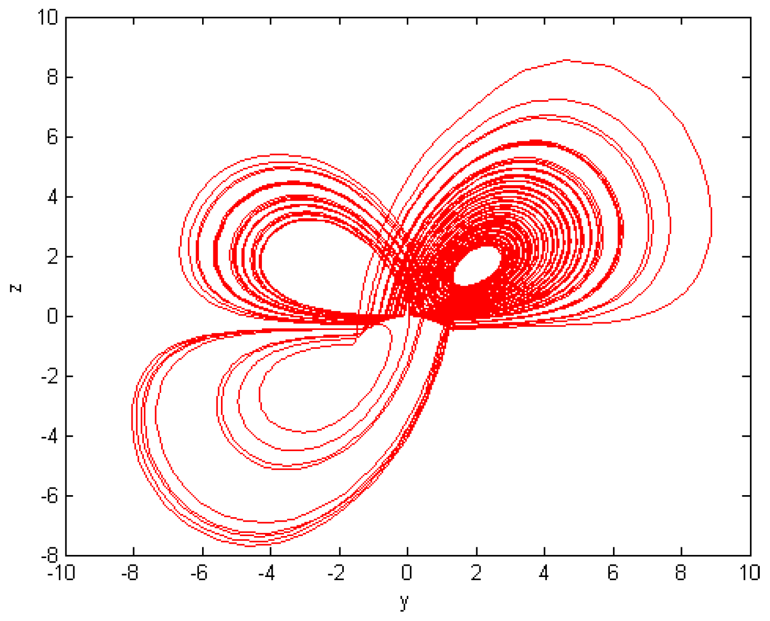
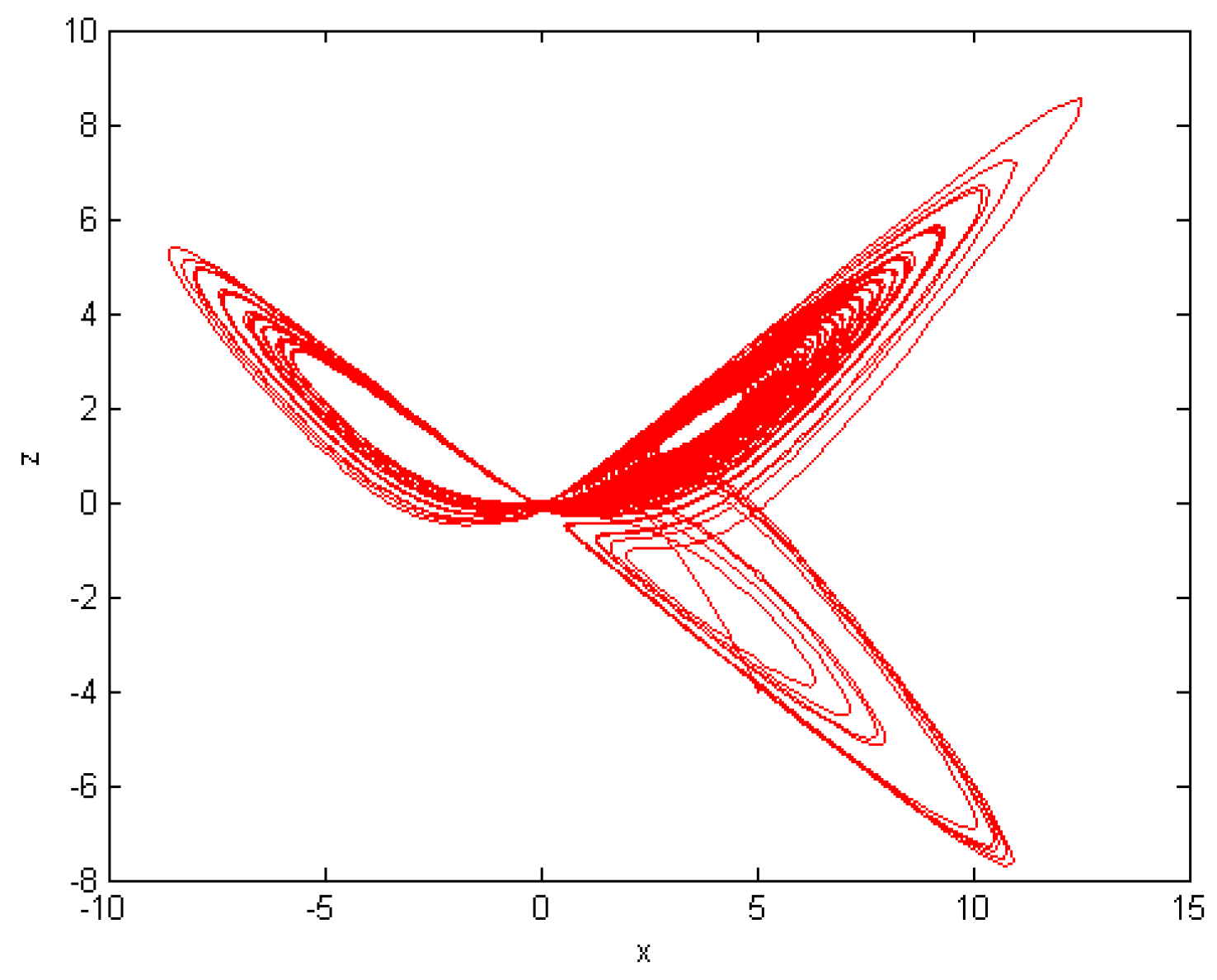
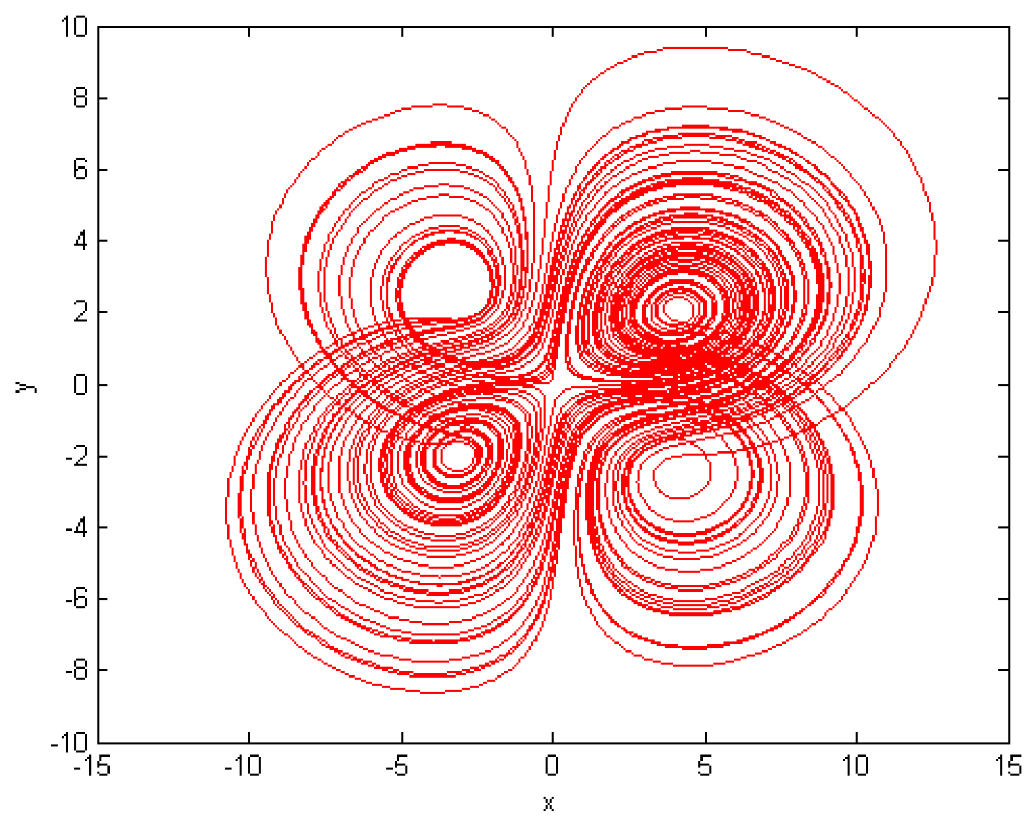
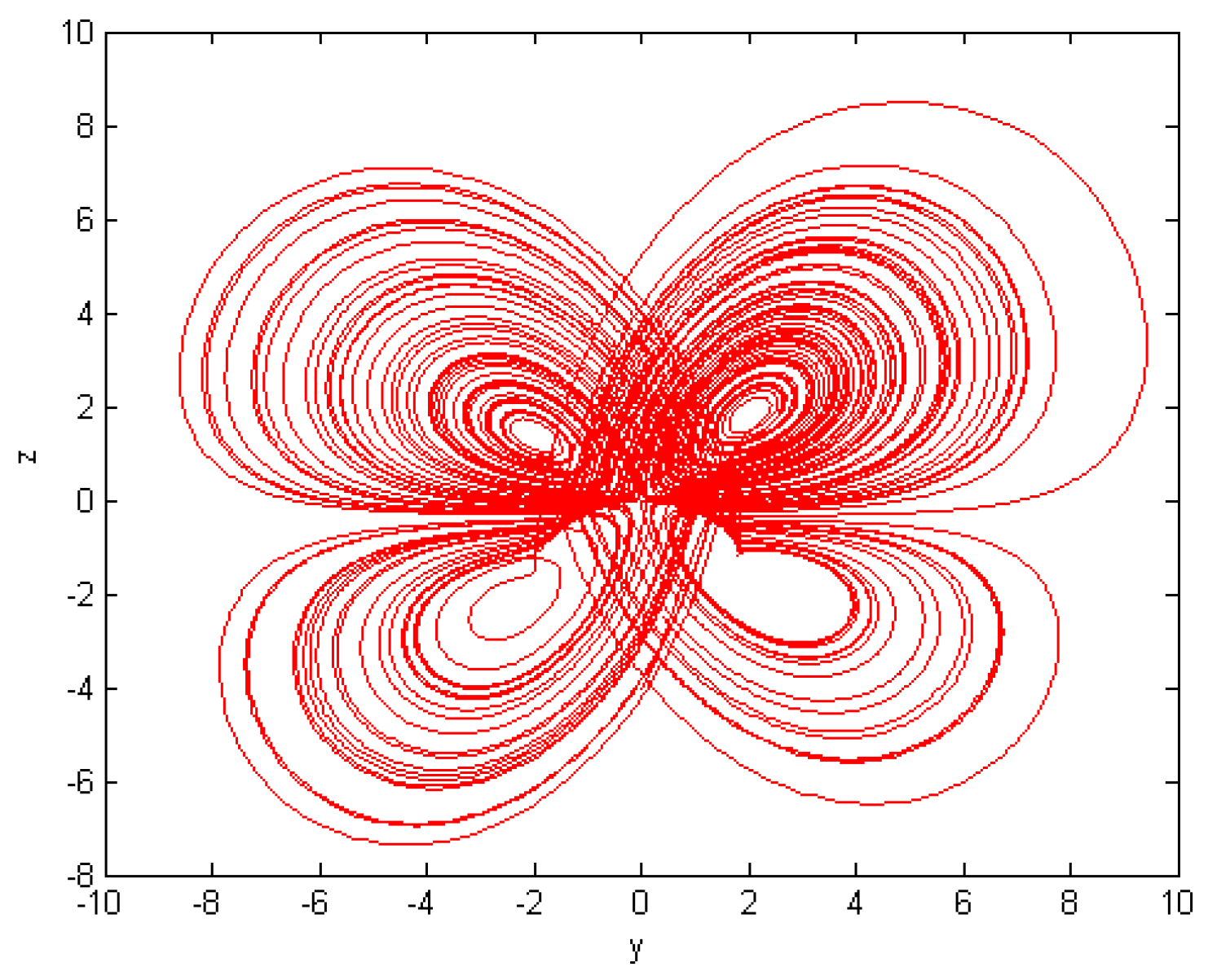
5. Numerical Results

In this section, the Atangana–Baleanu fractional derivative is approximated with the method of a Two-Step Lagrange polynomial from considering six cases on the Dadras–Momeni system under the fraction order chaotic dynamics. If we keep the initial states as they are and just vary one parameter, then a multi-scroll attractor will generate, which indicates that a system with high sensitive parameters changes the nature of chaotic systems. The Atangana–Baleanu fractional derivative has become one of most important tools to describe more generalization and memory-like real behaviors than classical differentiation. Its significance lies in its ability to model complex systems with greater precision, especially in circumstances where traditional calculus falls short, such as in anomalous diffusion, viscoelasticity, and thermal dynamics. In this paper, we use the derivative in one specific system in Dadras–Momeni systems to explore various complex chaotic behaviors resulting from its synchronization, such as multi-scroll attractors which are very important for secure communication and encryption applications. Our numerical approximation is ultimately implemented using the Two-Step Lagrange method, providing a very optimized solution and thereby facilitating easy multi-scroll chaotic attractors obtained by varying only one parameter, once again showing how flexible this system could be when subjected to fractional dynamics. The present work not only extends the theoretical knowledge concerning fractional chaotic systems, but it also highlights significance of Atangana–Baleanu derivatives in a practical aspect as well.

Case 1: For $\alpha =3,\beta =2.7,\delta =1.98,\eta =2$, and $\mu =9$ with initial conditions $x\left(0\right)=5,$ $y\left(0\right)=0$, and $z\left(0\right)=-4$, observe the formation of one scroll in Figure 1, Figure 2, Figure 3 and Figure 4:

Case 2: Keeping all parameters and initial conditions the same, except for $\delta =2.111225$, we observe the emergence of two scrolls in Figure 5, Figure 6, Figure 7 and Figure 8:

Case 3: With all parameters and initial conditions unchanged, except for $\delta =2.18892$, three scrolls start to appear, as shown in Figure 9, Figure 10, Figure 11 and Figure 12:

Case 4: All parameters and initial conditions are kept constant, except for $\delta =2.8$, leading to the formation of four scrolls, as illustrated in Figure 13, Figure 14, Figure 15 and Figure 16;

Case 5: Assuming all parameters and initial conditions remain the same, except for $\delta =3.9$, we observe an increased visibility of four scrolls, as depicted in Figure 17, Figure 18, Figure 19 and Figure 20:

Case 6: With all parameters and initial conditions held constant, except for $\delta =4.7$, four scrolls are observed, as illustrated in Figure 21, Figure 22, Figure 23 and Figure 24:

Comparison: The plotting of the fractional-order Dadras–Momeni system 7 using the Atangana–Baleanu fractional derivative, approximated with the Two-Step Lagrange polynomial, provides a comprehensive view of chaotic dynamics across varying parameter values for the fractional order $\hslash =0.98$ and different values of $\delta$. This research examines six situations where each distinct $\delta$ value generates unique scroll patterns in the $x-y,y-z,x-z$ phase planes, and in the 3D space $x-y-z$. In the first scenario, with $\delta =1.98$, we find a single scroll pattern in all phase planes, indicating substantially chaotic behavior, where interactions between variables produce complicated loops. This configuration oscillates around numerous equilibria, illustrating the system’s inclination to stabilize but occasionally wander, emphasizing its mild chaotic nature. In the second case, with $\delta =2.111225$, the system grows to two scrolls, demonstrating increased complexity as more oscillatory behavior emerges in the $x-y,y-z$, and $x-z$ phase plots, with each scroll indicating different regions of chaotic equilibrium. The third case with $\delta =2.18892$ produces three scrolls, indicating a further shift towards more pronounced chaotic dynamics. The increasing scroll number indicates that the system’s variables interact more intricately, resulting in a dense pattern of loops that confound phase pictures and time series behavior. Four scrolls are formed in the fourth and fifth examples, where $\delta =2.8$ and $\delta =3.9$, correspondingly. The additional scrolls form denser and more interwoven loops in the $x-y,y-z$ and $x-z$ phase planes. The time series analysis for these examples reveals increased oscillatory behavior, with more frequent transitions between states, indicating a greater sensitivity to initial conditions and a more evident chaotic nature. In the sixth scenario, with $\delta =4.7$, the four scrolls are clearly formed and demonstrate even clearer chaotic dynamics with high density and complicated interactions within the scrolls. Comparing these scenarios reveals how fractional order and the parameter $\delta$ affect the system’s chaotic dynamics. As $\delta$ grows, the number of scrolls and their density increase, creating a highly sensitive and unpredictable system. The graphical difference is in the density and quantity of scrolls, with situations with more scrolls (such as the fourth and fifth) displaying more chaotic transitions and stability thresholds. This comparison highlights how differences in $\delta$ and fractional-order parameters affect the complexity and sensitivity of the Dadras–Momeni system, demonstrating its adaptability in modeling dynamic, chaotic phenomena.

Conclusion: In summary, our research has been driven by incredible advances in chaos theory, fraction calculation, and fixed point theory. Together, they provide a robust framework for analyzing complex dynamic systems. By taking advantage of Atanga–Balenu fractional derivatives, we will be able to delve deeper into the context of fractional calculations. This framework uses these powerful tools to establish the existence and uniqueness of the system to create a rigorous mathematical basis through the lens of ${\theta }_{\mathbb{R}}$-contraction. This approach preserves the existence and uniqueness of the fixed points. It allows us to integrate and extend existing results in the literature on all metric areas. We also examine the graphical behavior of the chaotic system and the Dadras–Momeni fractional order by approximating the partial derivatives of Atanga–Balenu using the two-step Lagrangian polynomial method. This estimation provides valuable insights into the system dynamics at different scales—revealing new dimensions of nature. With this combined approach, our work provides a comprehensive analysis of complex systems. This facilitates a deeper understanding of chaotic dynamics within the framework of fractal computation and chaos theory.

Open Question: Bifurcation analysis of the fractional-order Dadras–Momeni system remains an intriguing area for further exploration. Researchers interested in this topic can refer to methodologies and insights provided in [28]. How do changes in the fractional order and key system parameters influence the bifurcation behavior of the Dadras–Momeni system? This question offers opportunities to uncover new dynamics and expand the understanding of fractional-order chaotic systems.

References

1. Banach, S. Sur les opérations dans les ensembles abstraits et leur application aux équations intégrales. Fundam. Math. 1922, 3, 133–181. [Google Scholar] [CrossRef]
2. Bakhtin, I.A. The contraction mapping principle in quasi-metric spaces. Funct. Anal. Unianowsk Gos. Ped. Inst. 1989, 30, 26–37. [Google Scholar]
3. Czerwik, S. Contraction mappings in b-metric spaces. Acta Math. Inform. Univ. Ostrav. 1993, 1, 5–11. [Google Scholar]
4. Kamran, T.; Samreen, M.; UL Ain, Q. A Generalization of b-Metric Space and Some Fixed Point Theorems. Mathematics 2017, 5, 19. [Google Scholar] [CrossRef]
5. Mlaiki, N.; Aydi, H.; Souayah, N.; Abdeljawad, T. Controlled Metric Type Spaces and the Related Contraction Principle. Mathematics 2018, 6, 194. [Google Scholar] [CrossRef]
6. Abdeljawad, T.; Mlaiki, N.; Aydi, H.; Souayah, N. Double controlled metric type spaces and some fixed point results. Mathematics 2018, 6, 320. [Google Scholar] [CrossRef]
7. Younis, M.; Ahmad, H.; Chen, L.; Han, M. Computation and convergence of fixed points in graphical spaces with an application to elastic beam deformations. J. Geom. Phys. 2023, 192, 104955. [Google Scholar] [CrossRef]
8. Ahmad, H.; Din, F.U.; Younis, M. A fixed point analysis of fractional dynamics of heat transfer in chaotic fluid layers. J. Comput. Appl. Math. 2025, 453, 116144. [Google Scholar] [CrossRef]
9. Younıs, M.; Mutlu, A.; Ahmad, H. Ćirić Contraction with Graphical Structure of Bipolar Metric Spaces and Related Fixed Point Theorems. Hacet. J. Math. Stat. 2024, 1–19. [Google Scholar] [CrossRef]
10. Ahmad, H. Analysis of Fixed Points in Controlled Metric Type Spaces with Application. In Recent Developments in Fixed-Point Theory: Theoretical Foundations and Real-World Applications; Springer Nature: Singapore, 2024; pp. 225–240. [Google Scholar]
11. Poincaré, H. Sur le problème des trois corps et les équations de la dynamique. Acta Math. 1890, 13, 1–270. [Google Scholar]
12. Lorenz, E.N. Deterministic nonperiodic flow. J. Atmos. Sci. 1963, 20, 130–141. [Google Scholar] [CrossRef]
13. May, R.M. Simple mathematical models with very complicated dynamics. Nature 1976, 261, 459–467. [Google Scholar] [CrossRef]
14. Feigenbaum, M.J. Quantitative universality for a class of nonlinear transformations. J. Stat. Phys. 1978, 19, 25–52. [Google Scholar] [CrossRef]
15. Mandelbrot, B.B. The Fractal Geometry of Nature; WH Freeman and Company: New York, NY, USA, 1982. [Google Scholar]
16. Liouville, J. Mémoire sur quelques questions de géométrie et de mécanique, et sur un nouveau genre de calcul pour résoudre ces questions. J. De L’École Polytech. 1832, 13, 1–69. [Google Scholar]
17. Caputo, M. Linear models of dissipation whose Q is almost frequency independent. II. Geophys. J. Int. 1967, 13, 529–539. [Google Scholar] [CrossRef]
18. Caputo, M.; Fabrizio, M. A new definition of fractional derivative without singular kernel. Prog. Fract. Differ. Appl. 2015, 1, 1–3. [Google Scholar]
19. Atangana, A.; Baleanu, D. New fractional derivatives with non-local and non-singular kernel, Theory and application to heat transfer model. Therm. Sci. 2016, 20, 763–769. [Google Scholar] [CrossRef]
20. Jleli, M.; Samet, B. A new generalization of the Banach contraction principle. J. Inequal. Appl. 2014, 38, 1–8. [Google Scholar] [CrossRef]
21. Branciari, A. A fixed point theorem of Banach-Caccioppoli type on a class of generalized metric spaces. Publ. Math. (Debr.) 2000, 57, 31–37. [Google Scholar] [CrossRef]
22. Jleli, M.; Karapınar, E.; Samet, B. Further generalizations of the Banach contraction principle. J. Inequal. Appl. 2014, 439, 1–9. [Google Scholar] [CrossRef]
23. Ahmad, J.; Al-Mazrooeia, A.E.; Cho, Y.J.; Yang, Y. Fixed point results for generalized θR-contractions. J. Nonlinear Sci. Appl. 2017, 10, 2350–2358. [Google Scholar] [CrossRef]
24. Liu, X.; Chang, S.; Xiao, Y.; Zao, L.C. Existence of fixed points for θR-type contraction and θR-type Suzuki contraction in complete metric spaces. Fixed Point Theory Appl. 2016, 8, 1–12. [Google Scholar]
25. Hussain, N.; Parvaneh, V.; Samet, B.; Vetro, C. Some fixed point theorems for generalized contractive mappings in complete metric spaces. Fixed Point Theory Appl. 2015, 185, 1–17. [Google Scholar] [CrossRef]
26. CvetkoviĆ, M.; Karapinar, E.; PetruŞel, A. Fixed point theorems for basic θ-contraction and applications. Carpathian J. Math. 2024, 40, 3–789. [Google Scholar] [CrossRef]
27. Dadras, S.; Momeni, H.R. A novel three-dimensional autonomous chaotic system generating two, three and four-scroll attractors. Phys. Lett. A 2009, 373, 3637–3642. [Google Scholar] [CrossRef]
28. Liu, X.; Hong, L.; Dang, H.; Yang, L. Bifurcations and Synchronization of the Fractional-Order Bloch System. Discret. Dyn. Nat. Soc. 2017, 2017, 4694305. [Google Scholar] [CrossRef]
Figure 1. Phase portrait of x-y plane.
Fractalfract 08 00699 g001
Figure 2. Phase portrait of y-z plane.
Fractalfract 08 00699 g002
Figure 3. Phase portrait of x-z plane.
Fractalfract 08 00699 g003
Figure 4. Phase portrait of x-y-z plane.
Fractalfract 08 00699 g004
Figure 5. Phase portrait of x-y plane.
Fractalfract 08 00699 g005
Figure 6. Phase portrait of y-z plane.
Fractalfract 08 00699 g006
Figure 7. Phase portrait of x-z plane.
Fractalfract 08 00699 g007
Figure 8. Phase portrait of x-y-z plane.
Fractalfract 08 00699 g008
Figure 9. Phase portrait of x-y plane.
Fractalfract 08 00699 g009
Figure 10. Phase portrait of y-z plane.
Fractalfract 08 00699 g010
Figure 11. Phase portrait of x-z plane.
Fractalfract 08 00699 g011
Figure 12. Phase portrait of x-y-z plane.
Fractalfract 08 00699 g012
Figure 13. Phase portrait of x-y plane.
Fractalfract 08 00699 g013
Figure 14. Phase portrait of y-z plane.
Fractalfract 08 00699 g014
Figure 15. Phase portrait of x-z plane.
Fractalfract 08 00699 g015
Figure 16. Phase portrait of x-y-z plane.
Fractalfract 08 00699 g016
Figure 17. Phase portrait of x-y plane.
Fractalfract 08 00699 g017
Figure 18. Phase portrait of y-z plane.
Fractalfract 08 00699 g018
Figure 19. Phase portrait of x-z plane.
Fractalfract 08 00699 g019
Figure 20. Phase portrait of x-y-z plane.
Fractalfract 08 00699 g020
Figure 21. Phase portrait of x-y plane.
Fractalfract 08 00699 g021
Figure 22. Phase portrait of y-z plane.
Fractalfract 08 00699 g022
Figure 23. Phase portrait of x-z plane.
Fractalfract 08 00699 g023
Figure 24. Phase portrait of x-y-z plane.
Fractalfract 08 00699 g024
Disclaimer/Publisher’s Note: The statements, opinions and data contained in all publications are solely those of the individual author(s) and contributor(s) and not of MDPI and/or the editor(s). MDPI and/or the editor(s) disclaim responsibility for any injury to people or property resulting from any ideas, methods, instructions or products referred to in the content.