Control of the Bifurcation Behaviors of Delayed Fractional-Order Neural Networks with Cooperation–Competition Topology

Abstract

In the real world, the competition and cooperation relationship exists in numerous systems. For instance, the competition–cooperation structure of a biological neural network is determined by the excitatory and inhibitory effects of neurons. The dynamic behaviors of a neural network model with a competition–cooperation structure are studied in this article, focusing particularly on the bifurcation and control problems. By selecting time delay as the parameter, a new sufficient condition for Hopf bifurcation is given and the impact of the fractional order on bifurcation behavior is determined for the network. Furthermore, a time-delay feedback controller is introduced to manage Hopf bifurcation behaviors, and, meanwhile, the stability domain is expanded. Our findings indicate that both fractional order and time delay play a crucial role in controlling the stability and Hopf bifurcation of the given model. Lastly, the accuracy of our theoretical results is verified through several numerical simulations, and the impact of control parameters on the bifurcation behavior of the network model is discussed in detail.

1. Introduction

Neural networks, mathematical models inspired by biological neural networks, consist of numerous interconnected neurons forming a highly nonlinear dynamic system. They are extensively utilized in diverse fields, such as pattern recognition, data mining, image processing, and natural language processing, to address complex problems [1,2,3,4,5,6,7]. The functionality of these networks largely depends on their system dynamics properties. For instance, the associative memory and optimization computing power of famous networks directly rely on the global stability of network dynamics. Consequently, the dynamic behaviors of neural networks have attracted considerable interest from scholars across various fields and have yielded a wealth of research findings. He et al. [8] introduced a novel full-dimensional nonlinear state feedback control strategy to optimize neural dynamics, then established conditions for local stability and Hopf bifurcation in binary-tree-structure and multi-delay diffusion neural network models. Lu et al. [9] constructed a new delayed neural network with a radial ring structure and bidirectional coupling, and they studied its stability and Hopf bifurcation dynamic behavior. Nie et al. [10] addressed the problem of coexistence and the dynamical behaviors of multiple equilibria for competitive neural networks.

Despite the significant interest in neural network dynamics in recent years, most research has focused only on the cooperation aspect of neuron relationships, neglecting the competition aspect present in neurons with negative connection weights. Competition is a ubiquitous phenomenon in daily life, manifesting in social networks as hostile or friendly relationships between individuals. Cooperation–competition topology networks have a wide range of specific applications, such as financial market prediction, intelligent optimization, and social network analysis [11,12,13]. Similarly, in neural networks, neurons can regulate information transmission through both promotion and inhibition, making it unrealistic to consider only cooperative scenarios. Therefore, studying neural networks with a cooperation–competition relationship [14,15,16,17] provides a more accurate reflection of real-world conditions. Exploring how to use the cooperation–competition structure of neural networks to study system dynamics is a worthwhile endeavor.

Fractional calculus, as an extension of classical integer-order differential and integral calculus, has sparked great interest, due to its potential applications in various fields, such as bioengineering, robotics, control, and medical problems. The memory and inheritance characteristics of different materials and processes in fractional-order differential equations make them more accurate than integer-order models when modeling real-world phenomena. Therefore, fractional calculus has been integrated into neural networks. Over the past few years, stability analysis, bifurcation and chaos, synchronization, and other properties of fractional-order dynamic systems have received increasing attention, leading to many significant achievements. Xu et al. [18] studied the problem of exponential bipartite synchronization of fractional-order multilayer signed networks via hybrid impulsive control. Siami [19] provided the classical secant condition for the stability analysis of cyclic interconnected commensurate fractional-order systems. Li et al. [20] investigated the stability control of fractional-order memory resistive neural networks with reaction–diffusion terms. Yin et al. [21] analyzed the discrete fractional-order LIF model and found that by adjusting the fractional order, neurons and neural network primitives can independently respond to weak signals at a certain frequency, enabling network primitives to achieve ordered cluster discharge. Huang et al. [22] investigated the bifurcation problem in a class of two delayed fractional-order neural networks with three neurons.

Among these efforts, the aim of bifurcation control is to design a controller capable of modifying bifurcation characteristics to achieve desirable dynamic behaviors. And the design and application of fractional-order control systems have always been highly concerned [23,24]. References [25,26,27,28] studied the fractional-calculus observer of the Lipschitz system and used the obtained state estimation for the final feedback control, providing insights for the control method of fractional-order systems with time delay and laying the foundation for fractional calculus and its application in neural networks. There have also been several studies on the application of bifurcation control controllers in different fields [29,30,31,32,33]. Cheng et al. [34] proposed a hybrid control strategy and considered the problem of Hopf bifurcation control for a complex network model with time delays. Lin et al. [35] studied a four-dimensional fractional-order two-gene regulatory network with multiple delays, and they introduced a fractional-order PD controller to maintain the stability of the network. Lu et al. [36] developed a fractional-order proportional–derivative controller to manage the bifurcation of a delayed fractional-order predator–prey system, effectively postponing the occurrence of Hopf bifurcation through the appropriate setting of control parameters. Wang et al. [37] designed a new hybrid controller, applying negative feedback control and time-delay feedback control, to regulate a dual-delay internet congestion control system accessed by a single resource. Based on the above research, it has proven necessary to introduce topological structures into neural networks for research, especially in the field of competition and cooperation.

Motivated by this framework, we incorporated graph theory into a multi-delay network model featuring cooperation–competition interactions, as a signed graph has both positive and negative interactions. Then, a bifurcation analysis was conducted on a delayed fractional-order neural network with a generalized cooperation–competition topology. This work offers several key contributions:

(1) The Caputo fractional derivative was employed, to expand the delayed neural network model with a generalized cooperation–competition topology into a fractional order model.

(2) The introduction of directed graphs concretizes the competitive–cooperation relationships. Unlike previous studies, we used graph connectivity to describe the relationships between neurons where the connectivity matrix plays a crucial role.

(3) Based on the connection relationship of the directed graph, the ranges of $\alpha$ and $\beta$ were determined, to provide sufficient conditions for the stability and Hopf bifurcation of the cooperative competitive network, with time delay as the bifurcation parameter.

(4) To postpone the occurrence of Hopf bifurcation, a nonlinear delay feedback controller was designed for a delayed fractional-order neural network model with a generalized cooperation–competition topology.

The rest of the paper is organized as follows. Section 2 introduces Caputo fractional-order derivatives and some fundamental theoretical concepts. A delayed fractional-order neural network model with a generalized cooperation–competition topology is established in Section 3. In Section 4, the stability of uncontrolled systems and the existence conditions of Hopf bifurcation are investigated. The dynamic behavior of the system after implementing a time-delay feedback controller are also discussed. In Section 5, several numerical simulations are conducted to validate the previously obtained theoretical results. The effects of fractional-order and controller parameters on system dynamics are analyzed. Our conclusions are summarized in Section 6.

2. Preliminaries

Definition 1 

([38]). The Caputo fractional-order derivative operator is defined as follows:

$${}_0{}^{c}D_x^{\varphi }f\left(x\right)={\displaystyle \frac{1}{\Gamma (n-\varphi )}}{\int }_0^x{(x-s)}^{n-\varphi -1}{f}^{\left(n\right)}\left(s\right)ds$$

where $n-1<\varphi <n$, when $k\in Z^{+}$. In particular, when $0<\varphi <1$,

$${}_0{}^{c}D_x^{\varphi }f\left(x\right)={\displaystyle \frac{1}{\Gamma (1-\varphi )}}{\int }_0^x{(x-s)}^{-\varphi }{f}^{\prime }\left(s\right)ds$$

Definition 2 

([38]). We give the Laplace transform of the Caputo fractional derivative, which is defined as

$$L{\{}_0^c{D}_x^{\varphi }f\left(x\right);s\}=s^{\varphi }F\left(s\right)-\sum _{l=0}^{k-1}{s}^{\varphi -l-1}{f}^{\left(l\right)}\left(0\right)$$

where $k-1\le \varphi \le k$ when $k\in Z^{+}$. If $f^{\left(l\right)}\left(0\right)=0,l=1,2,\dots ,n$ then $L{\{}_0^c{D}_x^{\varphi }f\left(x\right);s\}=s^{\varphi }F\left(s\right)$.

Next, we provide some basic concepts of a signed graph: a signed graph can be conveniently described by graphs $G=(Q,V,E)$, where $Q=\{q_1,q_2,...q_n\}$ represents the node set, and where $V\in Q\times Q=\left\{(q_i,q_j)\right|q_i,q_j\in Q\}$ represents the edge set. The matrix $E=\left[E_{ij}\right]\in R^{N\times N}$ is the adjacency matrix of a signed graph G, defined as follows: if $(q_i,q_j)\in V$ then $E_{ij}\ne 0$; if $(q_i,q_j)\notin V$ then $E_{ij}=0$. Due to the cooperation–competition relationship between nodes, there is the following definition: if the relationship between node $q_i$ and $q_j$ is competitive (cooperative) then $E_{ij}<0(E_{ij}>0)$.

Lemma 1. 

We consider an autonomous system $D^{q}x\left(t\right)=Bx\left(t\right)$; if all the eigenvalues $s_i(i=1,2,\dots n$) of $B={\left(b_{ij}\right)}_{nn}$ satisfy $|arg\left(s_i\right)|>{\displaystyle \frac{q\pi }{2}}$ and the characteristic equation $det(sI-B)=0$ has no purely imaginary roots for any $\tau >0$ then the zero solution of system is Lyapunov globally asymptotically stable.

Definition 3. 

If a node set Q of a signed graph can be divided into two subgroups $Q_1$ and $Q_2$, and if, among them, $Q_1$ and $Q_2$ meet $Q_1\cup Q_2=Q$ and $Q_1\cap Q_2=\varnothing$, so that $E_{ij}\ge 0$ for $\forall q_i,q_j\in Q_k(k\in 1,2)$ and $E_{ij}\le 0$ for $\forall q_i\in Q_k,q_j\in Q_{\xi }(k\ne \xi |k,\xi \in 1,2)$ then the signed graph is called a structural equilibrium graph.

Definition 4. 

The signum function is defined as

$$sgn\left(\epsilon \right)=\left\{\begin{array}{cc}\hfill -1,& \epsilon <0\hfill \\ \hfill 0,& \epsilon =0\hfill \\ \hfill 1,& \epsilon >0.\hfill \end{array}\right.$$

3. Model Description

Considering a complex dynamic neural network composed of N neurons, the state equations of each node in a delayed fractional order neural network with cooperation–competition topology can be described by the following differential equation:

$$\begin{array}{cc}\hfill D^{q_m}{x}_m\left(t\right)& =-a{x}_m\left(t\right)+bf\left(x_m\left(t\right)\right)+cf\left(x_m(t-{\tau }_m)\right)\hfill \\ \hfill & +d\sum _{n\in N_m}\left|G_{mn}\right|(sgn\left(G_{mn}\right)x_n\left(t\right)-x_m\left(t\right)),\hfill \end{array}$$

(1)

where $x_m\left(t\right)(m=1,2,\dots N)$ stand for the state of the mth neuron, a is the self-feedback coefficient, b and c is a constant and represents the connection weight, $d>0$ stands for the coupling strength, $f\left(x\right(·\left)\right)$ is the activation function, $\tau$ is the time delay at time t, $N_m$ is the neighbor set of node $x_m\left(t\right)$, and $G={\left(G_{mn}\right)}_{N\times N}$ denotes the symmetric adjacency matrix of the signed graph, describing the cooperation–competition interaction between neurons.

Remark 1. 

When there is a cooperative relationship between neuron m and neuron n, then $G_{mn}>0$. When there is a competitive relationship between neuron m and neuron n, then $G_{mn}<0$. Therefore, the term $G_{mn}(x_n\left(t\right)-x_m\left(t\right))$ represents the information exchange between the cooperation neighbor m and neuron n. For the convenience of analysis, we take $G_{mn}=\pm 1$.

Remark 2. 

When studying competition–cooperation relationships, the introduction of directed graphs concretizes competition–cooperation patterns. Unlike previous studies, we used graph connectivity to describe the relationships between neurons, whereas previous research used connectivity coefficients to describe the relationships between neurons, which made the model complex and difficult to implement. The method proposed in this paper is simple and highly feasible, with adjacency matrix $G={\left(G_{mn}\right)}_{N\times N}$ being a key factor.

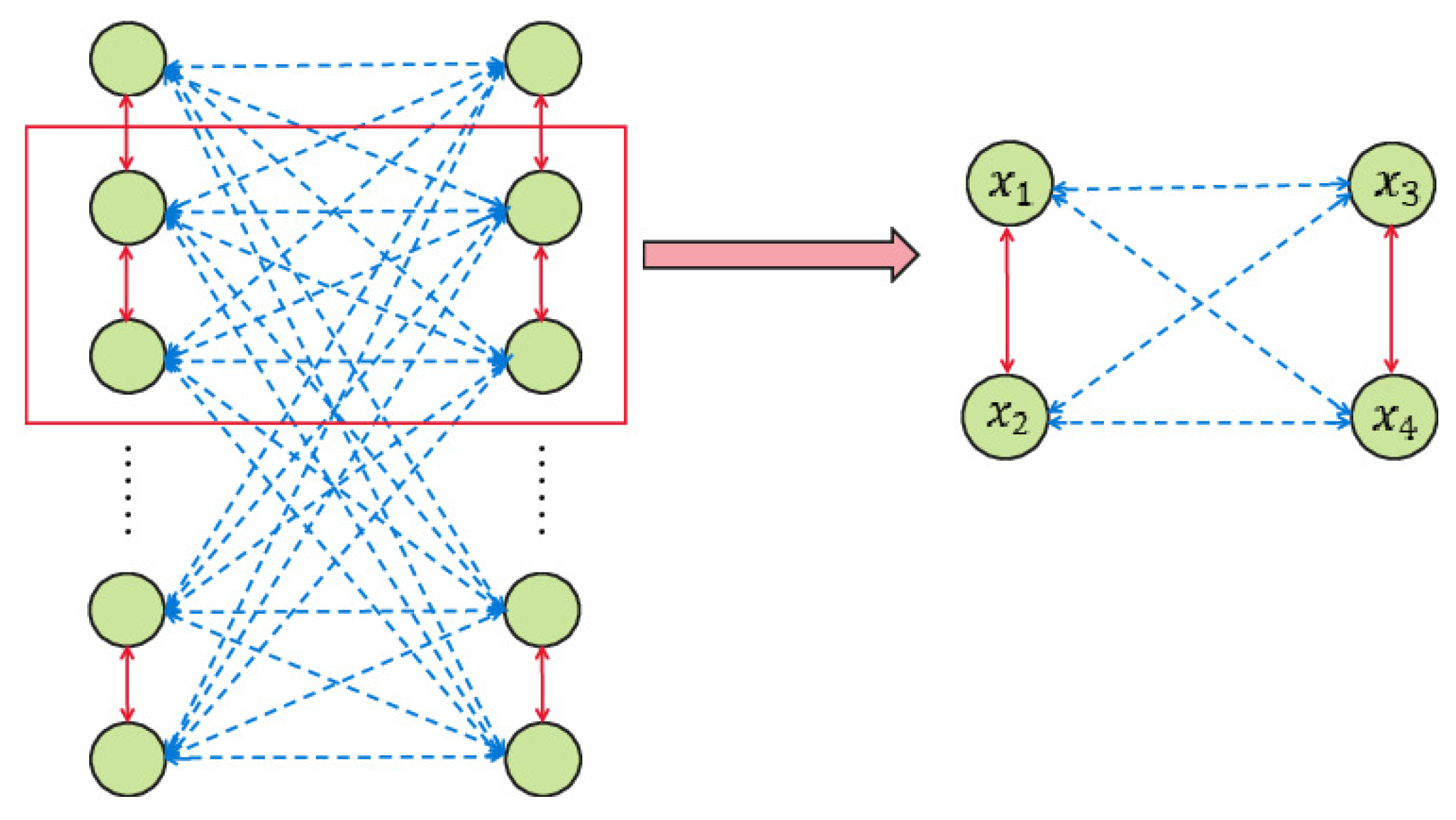
The structure of competition–cooperation is found in practice commonly. In a real neural network, it often contains a large number of neurons; usually, each neuron is independent but they interact with each other, which is a manifestation of the complexity of complex systems. Lower-dimensional neural networks are the foundation for understanding the dynamics of large-scale networks. This article mainly discusses a fractional-order neural network model with generalized cooperation–competition topology and four neurons. The topology diagram is shown in Figure 1. The solid line here represents the cooperative relationship between two neurons, while the dashed line represents the competitive relationship. So, the above system becomes

$$\left\{\begin{array}{cc}\hfill D^{q_1}{x}_1\left(t\right)& =-a{x}_1\left(t\right)+bf\left(x_1\left(t\right)\right)+cf\left(x_1(t-{\tau }_1)\right)\hfill \\ \hfill & +d(x_2\left(t\right)-x_1\left(t\right))-d(x_4\left(t\right)-x_1\left(t\right))\hfill \\ \hfill & -d(x_3\left(t\right)-x_1\left(t\right))\hfill \\ \hfill D^{q_2}{x}_2\left(t\right)& =-a{x}_2\left(t\right)+bf\left(x_2\left(t\right)\right)+cf\left(x_2(t-{\tau }_2)\right)\hfill \\ \hfill & +d(x_1\left(t\right)-x_2\left(t\right))-d(x_4\left(t\right)-x_2\left(t\right))\hfill \\ \hfill & -d(x_3\left(t\right)-x_2\left(t\right))\hfill \\ \hfill D^{q_3}{x}_3\left(t\right)& =-a{x}_3\left(t\right)+bf\left(x_3\left(t\right)\right)+cf\left(x_3(t-{\tau }_3)\right)\hfill \\ \hfill & +d(x_4\left(t\right)-x_3\left(t\right))-d(x_1\left(t\right)-x_3\left(t\right))\hfill \\ \hfill D^{q_4}{x}_4\left(t\right)& =-a{x}_4\left(t\right)+bf\left(x_4\left(t\right)\right)+cf\left(x_4(t-{\tau }_4)\right)\hfill \\ \hfill & -d(x_2\left(t\right)-x_3\left(t\right))\hfill \\ \hfill & +d(x_3\left(t\right)-x_4\left(t\right))-d(x_1\left(t\right)-x_4\left(t\right))\hfill \\ \hfill & -d(x_2\left(t\right)-x_4\left(t\right)).\hfill \end{array}\right.$$

(2)

For the convenience of analysis, we make the following assumptions:

(H1) 

$f\in C^R, f\left(0\right)=0, f^{\prime }\left(0\right)\ne 0,$

(H2) 

$\tau ={\tau }_1={\tau }_3={\tau }_2={\tau }_4$.

Figure 1. Topology diagram of neural networks with generalized cooperation–competition topology.

Figure 1. Topology diagram of neural networks with generalized cooperation–competition topology.

Remark 3. 

As is well known, the local stability and Hopf bifurcation threshold of a system depend on the linear part of the system. It is necessary for us to linearize network (2) and explore its stability conditions and bifurcation criteria hypothesis (H1). There is usually a time delay in the information transmission between neurons, which is reflected in network (2). Assumption (H2) actually indicates that the time delay between neurons is equal.

Remark 4. 

The adjacency matrix G is crucial in a cooperative–competitive topology relationship. If the competitive and cooperative topological relationship between neurons satisfies an asymmetric adjacency matrix then the model that satisfies the condition will be a simplified version of the model studied in this paper.

Obviously, it is easy to see that system (2) has a unique equilibrium point, which is defined as $E(0,0,0,0)$, so a Taylor expansion is performed on the nonlinear function $f\left(x\right(·\left)\right)$ at E, and its linear term is taken.

For this article, we mainly considered the study of the stability and Hopf bifurcation of system (3), and we used a delay feedback controller to delay the start of Hopf bifurcation and expand the stability domain of the system (3):

$$\left\{\begin{array}{cc}\hfill D^{q_1}{x}_1\left(t\right)& =-a{x}_1\left(t\right)+b^{\prime }{x}_1\left(t\right)+c^{\prime }{x}_1(t-\tau )\hfill \\ \hfill & +d(x_2\left(t\right)-x_1\left(t\right))-d(x_4\left(t\right)-x_1\left(t\right))\hfill \\ \hfill & -d(x_3\left(t\right)-x_1\left(t\right)),\hfill \\ \hfill D^{q_2}{x}_2\left(t\right)& =-a{x}_2\left(t\right)+b^{\prime }{x}_2\left(t\right)+c^{\prime }{x}_2(t-\tau )\hfill \\ \hfill & +d(x_1\left(t\right)-x_2\left(t\right))-d(x_4\left(t\right)-x_2\left(t\right))\hfill \\ \hfill & -d(x_3\left(t\right)-x_2\left(t\right)),\hfill \\ \hfill D^{q_3}{x}_3\left(t\right)& =-a{x}_3\left(t\right)+b^{\prime }{x}_3\left(t\right)+c^{\prime }{x}_3(t-\tau )\hfill \\ \hfill & +d(x_4\left(t\right)-x_3\left(t\right))-d(x_1\left(t\right)-x_3\left(t\right))\hfill \\ \hfill & -d(x_2\left(t\right)-x_3\left(t\right)),\hfill \\ \hfill D^{q_4}{x}_4\left(t\right)& =-a{x}_4\left(t\right)+b^{\prime }{x}_4\left(t\right)+c^{\prime }{x}_4(t-\tau )\hfill \\ \hfill & +d(x_3\left(t\right)-x_4\left(t\right))-d(x_1\left(t\right)-x_4\left(t\right))\hfill \\ \hfill & -d(x_2\left(t\right)-x_4\left(t\right)),\hfill \end{array}\right.$$

(3)

where $b^{\prime }={bf}^{\prime }\left(0\right)$, $c^{\prime }={cf}^{\prime }\left(0\right)$.

4. Main Results

For this section, we selected time delay as the bifurcation parameter, and we studied the stability and Hopf bifurcation of system (3) without control and with control, respectively. The following are the main results.

• A. Stability and Hopf bifurcation of the uncontrolled system.

In this segment, we mainly studied the dynamic behavior of (3) without control, and (3) is equivalent to (4):

$$\left\{\begin{array}{cc}\hfill D^{q_1}{x}_1\left(t\right)& =(-a+b^{\prime }-3d)x_1\left(t\right)+c^{\prime }{x}_1(t-\tau )+d{x}_2\left(t\right)\hfill \\ \hfill & -d{x}_3\left(t\right)-d{x}_4\left(t\right),\hfill \\ \hfill D^{q_2}{x}_2\left(t\right)& =d{x}_1\left(t\right)+(-a+b^{\prime }-3d)x_2\left(t\right)+c^{\prime }{x}_2(t-\tau )\hfill \\ \hfill & -d{x}_3\left(t\right)-d{x}_4\left(t\right),\hfill \\ \hfill D^{q_3}{x}_3\left(t\right)& =-d{x}_1\left(t\right)-d{x}_2\left(t\right)+(-a+b^{\prime }-3d)x_3\left(t\right)\hfill \\ \hfill & +c^{\prime }{x}_3(t-\tau )+d{x}_4\left(t\right),\hfill \\ \hfill D^{q_4}{x}_4\left(t\right)& =-d{x}_1\left(t\right)-d{x}_2\left(t\right)+d{x}_3\left(t\right)+(-a+b^{\prime }-3d)\hfill \\ \hfill & x_4\left(t\right)+c^{\prime }{x}_4(t-\tau ).\hfill \end{array}\right.$$

(4)

The characteristic matrix $\Delta \left(s\right)$ of system (4),

$$\begin{array}{c}\hfill \Delta \left(s\right)=\left[\begin{array}{cccc}{\Xi }_1& -d& d& d\\ -d& {\Xi }_2& d& d\\ d& d& {\Xi }_3& -d\\ d& d& -d& {\Xi }_4\end{array}\right]\end{array}$$

(5)

where $A=-a+b^{\prime }-3d$ and ${\Xi }_j=s^{q_j}-A-c^{\prime }{e}^{-s\tau }(j=1,2,3,4)$.

The characteristic equation corresponding to the above characteristic matrix is

$$\begin{array}{cc}\hfill & R_1\left(s\right)+R_2\left(s\right)e^{-s\tau }+R_3\left(s\right)e^{-2s\tau }+R_4\left(s\right)e^{-3s\tau }\hfill \\ \hfill & +R_5\left(s\right)e^{-4s\tau }=0,\hfill \end{array}$$

(6)

Multiplying $e^{2s\tau }$ on both sides of Equation (6), we can obtain

$$\begin{array}{c}\hfill R_1\left(s\right)e^{2s\tau }+R_2\left(s\right)e^{s\tau }+R_3\left(s\right)+R_4\left(s\right)e^{-s\tau }+R_5\left(s\right)e^{-2s\tau }=0,\end{array}$$

(7)

where $R_1\left(s\right)$, $R_2\left(s\right)$, $R_3\left(s\right)$, $R_4\left(s\right)$, $R_5\left(s\right)$ is a function about s; the detailed information is presented in Appendix A, abbreviated as $R_1$, $R_2$, $R_3$, $R_4$, $R_5$.

We define $R_{iR}$ and $R_{iI}$ as the real and imaginary part of $R_i(i=1,2,3,4,5)$, respectively. And we let $s=i\omega =\omega (cos{\displaystyle \frac{\pi }{2}}+isin{\displaystyle \frac{\pi }{2}})(\omega >0)$ be the root of Equation (7), and (7) can be transformed into (8):

$$\begin{array}{cc}\hfill & (R_{1R}+i{R}_{1I})(cos2\omega \tau +isin2\omega \tau )+(R_{2R}+i{R}_{2I})\hfill \\ \hfill & (cos\omega \tau +isin\omega \tau )+(R_{3R}\left(\omega \right)+i{R}_{3I})+(R_{4R}+i{R}_{4I})\hfill \\ \hfill & (cos\omega \tau -isin\omega \tau )+(R_{5R}+i{R}_{5I})(cos2\omega \tau -isin2\omega \tau )=0.\hfill \end{array}$$

(8)

Separating the real and imaginary parts, we obtain

$$\left\{\begin{array}{c}(R_{1R}+R_{5R})cos2\omega \tau +(R_{5I}-R_{1I})sin2\omega \tau +(R_{2R}+R_{4R})\hfill \\ cos\omega \tau +(R_{4I}-R_{2I})sin\omega \tau +R_{3R}=0,\hfill \\ (R_{1I}+R_{5I})cos2\omega \tau -(R_{5R}-R_{1R})sin2\omega \tau +(R_{2I}+R_{4I})\hfill \\ cos\omega \tau -(R_{4R}-R_{2R})sin\omega \tau +R_{3I}=0.\hfill \end{array}\right.$$

(9)

By introducing the trigonometric function formula $sin\omega \tau =\pm \sqrt{1-co{s}^2\omega \tau }$, $cos2\omega \tau =2co{s}^2\omega \tau -1$, $sin2\omega \tau =2sin\omega \tau cos\omega \tau =2cos\omega \tau \sqrt{1-co{s}^2\omega \tau }$, the first equation of Equation (9) can be transformed into

$$\begin{array}{cc}\hfill & (R_{1R}+R_{5R})(2co{s}^2\omega \tau -1)+(R_{2R}+R_{4R})cos\omega \tau +R_{3R}=\hfill \\ \hfill & -2(R_{5I}-R_{1I})cos\omega \tau \sqrt{1-co{s}^2\omega \tau }-(R_{4I}-R_{2I})\sqrt{1-co{s}^2\omega \tau }.\hfill \end{array}$$

(10)

Squaring both sides of Equation (10) makes it easy to obtain

$$\begin{array}{c}\hfill {\alpha }_{4}co{s}^4\omega \tau +{\alpha }_{3}co{s}^3\omega \tau +{\alpha }_{2}co{s}^2\omega \tau +{\alpha }_{1}cos\omega \tau +{\alpha }_0=0.\end{array}$$

(11)

Let $z=cos\omega \tau$; then, Equation (11) becomes

$$\begin{array}{c}\hfill {\alpha }_4{z}^4+{\alpha }_3{z}^3+{\alpha }_2{z}^2+{\alpha }_{1}z+{\alpha }_0=0.\end{array}$$

(12)

In the following, we need to find a condition that ensures that Equation (12) has at least one root. We define $g\left(z\right)={\alpha }_4{z}^4+{\alpha }_3{z}^3+{\alpha }_2{z}^2+{\alpha }_{1}z+{\alpha }_0$. From the above analysis, we can obtain the following lemma:

Lemma 2. 

If ${\alpha }_0<0$, i.e., ${(R_{1R}+R_{5R})}^2+R_{3R}^2-2R_{3R}(R_{1R}+R_{5R})-{(R_{4I}-R_{2I})}^2<0$ then Equation (11) has at least one positive root.

Proof. 

Through Equation (12), it can be seen that Equation (12) is a one-dimensional quartic equation about z. If ${\alpha }_0<0$ then $g\left(0\right)={\alpha }_0<0$. Also, ${\alpha }_4=4{(R_{1R}+R_{5R})}^2+4{(R_{5I}-R_{1I})}^2$ is a constant that is always greater than or equal to 0, and $\underset{z\to +\infty }{lim}g\left(z\right)=+\infty$. Therefore, at least one real value $z_0$ satisfies $g\left(z_0\right)=0$. Thus, it can be concluded that Equation (11) has at least one root $cos\omega \tau$. This complete the proof. □

We assume

$$\begin{array}{c}\hfill cos\omega \tau =h_1\left(\omega \right),\end{array}$$

(13)

where $h_1\left(\omega \right)$ is a continuous function about $\omega$.

Similarly, by applying the trigonometric function formula $cos2\omega \tau =1-2si{n}^2\omega \tau$, $sin2\omega \tau =2sin\omega \tau \sqrt{1-si{n}^2\omega \tau }$, the first equation of Equation (9) can be transformed into

$$\begin{array}{cc}\hfill & (R_{1R}+R_{5R})(1-2si{n}^2\omega \tau )+(R_{4I}-R_{2I})sin\omega \tau +R_{3R}=\hfill \\ \hfill & -2(R_{5I}-R_{1I})sin\omega \tau \sqrt{1-{sin}^2\omega \tau }-(R_{2R}+R_{4R})\sqrt{1-{sin}^2\omega \tau }.\hfill \end{array}$$

(14)

Squaring both sides of Equation (14) makes it easy to obtain

$$\begin{array}{c}\hfill {\beta }_4{sin}^4\omega \tau +{\beta }_3{sin}^3\omega \tau +{\beta }_2{sin}^2\omega \tau +{\beta }_{1}sin\omega \tau +{\beta }_0=0.\end{array}$$

(15)

Let $\varrho =sin\omega \tau$; then, Equation (15) becomes

$$\begin{array}{c}\hfill {\beta }_4{\varrho }^4+{\beta }_3{\varrho }^3+{\beta }_2{\varrho }^2+{\beta }_1\varrho +{\beta }_0=0.\end{array}$$

(16)

In the following, we need to find a condition that ensures that Equation (16) has at least one root. We denote $m\left(\varrho \right)={\beta }_4{\varrho }^4+{\beta }_3{\varrho }^3+{\beta }_2{\varrho }^2+{\beta }_1\varrho +{\beta }_0$. From the above analysis, we can obtain the following lemma:

Lemma 3. 

If ${\beta }_0<0$, i.e., ${(R_{1R}+R_{5R})}^2+R_{3R}^2+2R_{3R}(R_{1R}+R_{5R})-{(R_{2R}+R_{4R})}^2<0$ then Equation (15) has at least one root.

Proof. 

Through Equation (16), it can be seen that Equation (16) is a one-dimensional quartic equation about $\varrho$. If ${\beta }_0<0$ then $m\left(0\right)={\beta }_0<0<0$. Also, ${\beta }_4=4{(R_{1R}+R_{5R})}^2+4{(R_{5I}-R_{1I})}^2$ is a constant that is always greater than or equal to 0 and $\underset{\varrho \to +\infty }{lim}m\left(\varrho \right)=+\infty$. Therefore, at least one real value ${\varrho }_0$ satisfies $m\left({\varrho }_0\right)=0$. Thus, it can be concluded that Equation (15) has at least one root $sin\omega \tau$. This complete the proof. □

Remark 5. 

According to the theorem on the existence of roots in a quadratic equation, if ${\alpha }_0<0$ then $g\left(z\right)=0$ must have a root $z_0$ belonging to $(0,+\infty )$. Obviously, ${\alpha }_0<0$ is a sufficient condition for ensuring system stability. Similarly, ${\beta }_0<0$ is quite important.

We assume

$$\begin{array}{c}\hfill sin\omega \tau =h_2\left(\omega \right),\end{array}$$

(17)

where $h_2\left(\omega \right)$ is a continuous function about $\omega$.

From $si{n}^2\omega \tau +co{s}^2\omega \tau =1$, it can be seen that

$$\begin{array}{c}\hfill h_1^2\left(\omega \right)+h_2^2\left(\omega \right)=1.\end{array}$$

(18)

In view of $cos\omega \tau =h_1\left(\omega \right)$, we have

$$\begin{array}{c}\hfill {\tau }^{\kappa }={\displaystyle \frac{1}{\omega }}[arccos{h}_1\left(\omega \right)+2\kappa \pi ],\kappa =0,1,2,....\end{array}$$

(19)

Suppose Equation (18) has at least one positive real root.

Set

$$\begin{array}{c}\hfill {\tau }_0=min{\tau }^{\kappa },\kappa =0,1,2,\dots ,{\omega }_0{=\omega |}_{\tau ={\tau }_0}.\end{array}$$

(20)

In order to derive the conditions for the occurrence of the Hopf bifurcation, the following assumptions must be given:

(H3) 

$$\begin{array}{c}\hfill {\displaystyle \frac{D_{2R}{D}_{1R}+D_{2I}{D}_{1I}}{D_{1R}^2+D_{1I}^2}}\ne 0.\end{array}$$

(21)

Lemma 4. 

Let $s\left(\tau \right)=\zeta \left(\tau \right)+i\omega \left(\tau \right)$ be the root of (7) satisfying $\zeta \left({\tau }_0\right)=0$, $\omega \left({\tau }_0\right)={\omega }_0$. Then, the following transversality condition holds:

$$\begin{array}{c}\hfill Re[{\displaystyle \frac{ds}{d\tau }}]{|}_{\tau ={\tau }_0,\omega ={\omega }_0}\ne 0.\end{array}$$

Proof. 

Taking the derivative with respect to $\tau$ on both sides of Equation (7), we have

$$\begin{array}{cc}\hfill {\displaystyle \frac{ds}{d\tau }}& ={\displaystyle \frac{s(2(R_5{e}^{-2s\tau }-R_1{e}^{2s\tau })+(R_4{e}^{-s\tau }-R_2{e}^{s\tau })}{\begin{array}{c}{R}_3^{\prime }+R_1^{\prime }{e}^{2s\tau }+R_2^{\prime }{e}^{s\tau }+R_4^{\prime }{e}^{-s\tau }\\ -\tau (2(R_5{e}^{-2s\tau }-R_1{e}^{2s\tau })+(R_4{e}^{-s\tau }-R_2{e}^{s\tau }))\end{array}}},\hfill \end{array}$$

(22)

where $R_i^{\prime }(i=1,2,3,4,5)$ are the derivatives of $R_i$.

Then,

$$\begin{array}{cc}\hfill & {[{\displaystyle \frac{ds}{d\tau }}]}^{-1}={\displaystyle \frac{R_3^{\prime }+R_1^{\prime }{e}^{2s\tau }+R_2^{\prime }{e}^{s\tau }+R_4^{\prime }{e}^{-s\tau }}{s(2(R_5{e}^{-2s\tau }-R_1{e}^{2s\tau })+(R_4{e}^{-s\tau }-R_2{e}^{s\tau }))}}-{\displaystyle \frac{\tau }{s}}.\hfill \end{array}$$

(23)

Bringing $s=i{\omega }_0$ into (23), we have

$$\begin{array}{cc}\hfill & sign\{Re[{\displaystyle \frac{ds}{d\tau }}]{|}_{s=i{\omega }_0,\tau ={\tau }_0}\}=sign\{Re{[{\displaystyle \frac{ds}{d\tau }}]}^{-1}{|}_{s=i{\omega }_0,\tau ={\tau }_0}\}\hfill \end{array}$$

$$\begin{array}{c}\hfill Re{[{\displaystyle \frac{ds}{d\tau }}]}^{-1}{|}_{s=i{\omega }_0,\tau ={\tau }_0}\\ \hfill & =Re({\displaystyle \frac{D_2}{D_1}}){|}_{s=i{\omega }_0,\tau ={\tau }_0}\hfill \\ \hfill & ={\displaystyle \frac{D_{2R}{D}_{1R}+D_{2I}{D}_{1I}}{D_{1R}^2+D_{1I}^2}},\hfill \end{array}$$

(24)

where

$\left\{\begin{array}{c}{D}_1=s(2(R_5{e}^{-2s\tau }-R_1{e}^{2s\tau })+(R_4{e}^{-s\tau }-R_2{e}^{s\tau }))\hfill \\ D_2=R_3^{\prime }+R_1^{\prime }{e}^{2s\tau }+R_2^{\prime }{e}^{s\tau }+R_4^{\prime }{e}^{-s\tau }\hfill \end{array}\right.$ The detailed proof process will be presented in Appendix B.

Therefore, under the assumptions condition $\left(H3\right)$, we have

$$\begin{array}{c}\hfill Re[{\displaystyle \frac{ds}{d\tau }}]{|}_{s=i{\omega }_0,\tau ={\tau }_0}\ne 0.\end{array}$$

(25)

Thus, the transversality condition of system (2) near $\tau ={\tau }_0$ is satisfied. □

Next, we consider the dynamic behavior of the system when $\tau =0$. When there is no transmission delay in system (2), Equation (7) becomes

$$\begin{array}{c}\hfill s^4+{\theta }_1{s}^3+{\theta }_2{s}^2+{\theta }_{3}s+{\theta }_4=0,\end{array}$$

(26)

where

$$\left\{\begin{array}{cc}\hfill {\theta }_1& =-4(A+c^{\prime }),\hfill \\ \hfill {\theta }_2& =6(A^2-d^2+2A{c}^{\prime }+c^{\prime 2}),\hfill \\ \hfill {\theta }_3& =-4(A^3-3A{d}^2+2d^3+3A^2{c}^{\prime }-3c^{\prime }{d}^2+3A{c}^{\prime 2}+c^{\prime 3},\hfill \\ \hfill {\theta }_4& =A^4-6A^2{d}^2-3d^4+4A^3{c}^{\prime }-12A{c}^{\prime }{d}^2+6A^2{c}^{\prime 2}\hfill \\ \hfill & -6c^{\prime 2}{d}^2+4A{c}^{\prime 3}+c^{\prime 4}+8A{d}^3+8c^{\prime }{d}^3.\hfill \end{array}\right.$$

In order to obtain some of the main results of this article, we made the following assumptions:

(H4) 

${\theta }_4>0;{\theta }_1{\theta }_2>{\theta }_3;{\theta }_3({\theta }_1{\theta }_2-{\theta }_3)>{\theta }_1^2{\theta }_4.$

Lemma 5. 

Under assumption $\left(H4\right)$ and if $\tau =0$ then all the characteristic roots of characteristic Equation (26) have negative real parts. Therefore, system (2) is locally asymptotically stable without a time delay.

Proof. 

It follows the assumption $\left(H4\right)$ that all the roots $s_i$ of Equation (26) satisfy $|arg\left(s_i\right)|>{\displaystyle \frac{q_i\pi }{2}}(i=1,2,3,4)$. By Lemma 1, we can conclude, then, that all the characteristic roots of characteristic Equation (26) have no purely imaginary roots. Therefore, without the time delay, system (2) is locally asymptotically stable. □

Based on the above discussion, we can obtain the following main results:

Theorem 1. 

Assuming that system (2) satisfies hypothesis $\left(H1\right)$–$\left(H4\right)$ and satisfies conditions ${\alpha }_0<0$, ${\beta }_0<0$, the following statement holds:

(1) 

If $\left(H1\right)$ and $\left(H4\right)$ hold, system (2) is locally asymptotically stable when $\tau =0$.

(2) 

If $\left(H1\right)$, $\left(H2\right)$, $\left(H3\right)$, and ${\alpha }_0<0$, ${\beta }_0<0$ hold, system (2) is locally asymptotically stable when $\tau \in (0,{\tau }_0)$, and it is unstable for $\tau >{\tau }_0$. Then, system (2) undergoes Hopf bifurcation when $\tau ={\tau }_0$.

• B. Stability and Hopf bifurcation of the controlled system

In recent years, various controllers have been designed to address the Hopf bifurcation problem in controlling fractional-order systems. However, the exploration of the Hopf bifurcation control problem for fractional-order systems with cooperative–competitive topology is limited. To address this limitation, we introduced a time-delay feedback controller, as shown below:

$$\begin{array}{c}\hfill U\left(t\right)=K_1(X(t-\tau )-X\left(t\right)),\end{array}$$

(27)

where $K_1$ is the feedback gain coefficient.

Remark 6. 

In view of the general thought on polynomial function controllers, a nonlinear delayed feedback controller $U_1\left(t\right)={\displaystyle \sum _{i=1}^3}{K}_i{(X(t-\tau )-X\left(t\right))}^i$ was designed in reference [39]. We know that the linear term $K_1(X(t-\tau )-X\left(t\right))$ can change the beginning of the Hopf bifurcation in fractional order models, while the nonlinear terms $K_2{(X(t-\tau )-X\left(t\right))}^2$ and $K_3{(X(t-\tau )-X\left(t\right))}^3$ only affect the frequency and amplitude of bifurcation oscillation, and the feedback gain coefficient $K_2$ has little effect on the frequency of bifurcation oscillation, while $K_3$ has almost no effect. Therefore, we chose to introduce a time-delay feedback controller $U\left(t\right)=K_1(X(t-\tau )-X\left(t\right))$ for bifurcation control in this article.

We add the above controller to system (2); then, system (2) will be transformed into

$$\left\{\begin{array}{cc}\hfill D^{q_1}{x}_1\left(t\right)& =-a{x}_1\left(t\right)+bf\left(x_1\left(t\right)\right)+cf\left(x_1(t-{\tau }_1)\right)\hfill \\ \hfill & +d(x_2\left(t\right)-x_1\left(t\right))-d(x_4\left(t\right)-x_1\left(t\right))\hfill \\ \hfill & -d(x_3\left(t\right)-x_1\left(t\right))+K_1(x_1(t-\tau )-x_1\left(t\right)),\hfill \\ \hfill D^{q_2}{x}_2\left(t\right)& =-a{x}_2\left(t\right)+bf\left(x_2\left(t\right)\right)+cf\left(x_2(t-{\tau }_2)\right)\hfill \\ \hfill & +d(x_1\left(t\right)-x_2\left(t\right))-d(x_4\left(t\right)-x_2\left(t\right))\hfill \\ \hfill & -d(x_3\left(t\right)-x_2\left(t\right)),\hfill \\ \hfill D^{q_3}{x}_3\left(t\right)& =-a{x}_3\left(t\right)+bf\left(x_3\left(t\right)\right)+cf\left(x_3(t-{\tau }_3)\right)\hfill \\ \hfill & +d(x_4\left(t\right)-x_3\left(t\right))-d(x_1\left(t\right)-x_3\left(t\right))\hfill \\ \hfill & -d(x_2\left(t\right)-x_3\left(t\right)),\hfill \\ \hfill D^{q_4}{x}_4\left(t\right)& =-a{x}_4\left(t\right)+bf\left(x_4\left(t\right)\right)+cf\left(x_4(t-{\tau }_4)\right)\hfill \\ \hfill & +d(x_3\left(t\right)-x_4\left(t\right))-d(x_1\left(t\right)-x_4\left(t\right))\hfill \\ \hfill & -d(x_2\left(t\right)-x_4\left(t\right))+K_1(x_4(t-\tau )-x_4\left(t\right)).\hfill \end{array}\right.$$

(28)

Remark 7. 

Assuming node set $V=(x_1,x_2,x_3,x_4)$, it can be seen that node set V can be divided into two subsets $V_1$ and $V_2$ from definition 3. Therefore, we only need to control one node in each subset when adding control. For this article, we chose to add time-delay feedback controllers to the equations of node $x_1$ and node $x_4$ in system (2).

By the Taylor expansion of system (28), the linearization part of system (28) at the equilibrium point $E(0,0,0,0)$ can be obtained:

$$\left\{\begin{array}{cc}\hfill D^{q_1}{x}_1\left(t\right)& =(-a+b^{\prime }-3d-K_1)x_1\left(t\right)+(c^{\prime }+K_1)\hfill \\ \hfill & x_1(t-\tau )+d{x}_2\left(t\right)-d{x}_3\left(t\right)-d{x}_4\left(t\right),\hfill \\ \hfill D^{q_2}{x}_2\left(t\right)& =d{x}_1\left(t\right)+(-a+b^{\prime }-3d)x_2\left(t\right)+c^{\prime }{x}_2(t-\tau )\hfill \\ \hfill & -d{x}_3\left(t\right)-d{x}_4\left(t\right),\hfill \\ \hfill D^{q_3}{x}_3\left(t\right)& =-d{x}_1\left(t\right)-d{x}_2\left(t\right)+(-a+b^{\prime }-3d)x_3\left(t\right)\hfill \\ \hfill & +c^{\prime }{x}_3(t-\tau )+d{x}_4\left(t\right),\hfill \\ \hfill D^{q_4}{x}_4\left(t\right)& =-d{x}_1\left(t\right)-d{x}_2\left(t\right)+d{x}_3\left(t\right)+(-a+b^{\prime }-3d\hfill \\ \hfill & -K_1)x_4\left(t\right)+(c^{\prime }+K_1)x_4(t-\tau ).\hfill \end{array}\right.$$

(29)

The characteristic matrix ${\Delta }_1\left(s\right)$ of system (29),

$$\begin{array}{c}\hfill {\Delta }_1\left(s\right)=\left[\begin{array}{cccc}{\Lambda }_1& -d& d& d\\ -d& {\Xi }_2& d& d\\ d& d& {\Xi }_3& -d\\ d& d& -d& {\Lambda }_4\end{array}\right]\end{array}$$

(30)

where $A=-a+b^{\prime }-3d$, $B=-a+b^{\prime }-3d-K_1$, $G=c^{\prime }+K_1$, and ${\Lambda }_{\ell }=s^{q_{\ell }}-B-G{e}^{-s\tau },(\ell =1,4)$.

The characteristic equation corresponding to the above characteristic matrix is

$$\begin{array}{c}\hfill {\eta }_1\left(s\right)+{\eta }_2\left(s\right)e^{-s\tau }+{\eta }_3\left(s\right)e^{-2s\tau }+{\eta }_4\left(s\right)e^{-3s\tau }+{\eta }_5\left(s\right)e^{-4s\tau }=0,\end{array}$$

(31)

where ${\eta }_1\left(s\right)$, ${\eta }_2\left(s\right)$, ${\eta }_3\left(s\right)$, ${\eta }_4\left(s\right)$, ${\eta }_{(}s)$ is a function about s, abbreviated as ${\eta }_1$, ${\eta }_2$, ${\eta }_3$, ${\eta }_4$, ${\eta }_5$ in subsequent articles.

Multiplying $e^{2s\tau }$ on both sides of Equation (31), we can obtain

$$\begin{array}{c}\hfill {\eta }_1{e}^{2s\tau }+{\eta }_2{e}^{s\tau }+{\eta }_3+{\eta }_4{e}^{-s\tau }+{\eta }_5{e}^{-2s\tau }=0.\end{array}$$

(32)

We define ${\eta }_{iR}$ and ${\eta }_{iI}$ as the real and imaginary part of ${\eta }_i(i=1,2,3,4,5)$, respectively. Then, Equation (32) is equivalent to

$$\begin{array}{cc}\hfill & ({\eta }_{1R}+{\eta }_{1I})e^{2s\tau }+({\eta }_{2R}+{\eta }_{2I})e^{s\tau }+({\eta }_{3R}+{\eta }_{3I})\hfill \\ \hfill & +({\eta }_{4R}+{\eta }_{4I})e^{-s\tau }+({\eta }_{5R}+{\eta }_{5I})e^{-2s\tau }=0.\hfill \end{array}$$

(33)

We let $s=i\omega =\omega (cos{\displaystyle \frac{\pi }{2}}+isin{\displaystyle \frac{\pi }{2}})(\omega >0)$ be the root of Equation (31), and we substitute $s=i\omega =\omega (cos{\displaystyle \frac{\pi }{2}}+isin{\displaystyle \frac{\pi }{2}})$ into Equation (31) to obtain

$$\begin{array}{cc}\hfill & ({\eta }_{1R}+i{\eta }_{1I})(cos2\omega \tau +isin2\omega \tau )+({\eta }_{2R}+i{\eta }_{2I})(cos\omega \tau +\hfill \\ \hfill & isin\omega \tau )+({\eta }_{3R}+i{\eta }_{3I})+({\eta }_{4R}+i{\eta }_{4I})(cos\omega \tau -isin\omega \tau )+\hfill \\ \hfill & ({\eta }_{5R}+i{\eta }_{5I})(cos2\omega \tau -isin2\omega \tau )=0.\hfill \end{array}$$

(34)

Separating the real and imaginary parts, we obtain

$$\left\{\begin{array}{c}({\eta }_{1R}+{\eta }_{5R})cos2\omega \tau +({\eta }_{5I}-{\eta }_{1I})sin2\omega \tau +({\eta }_{2R}+{\eta }_{4R})\hfill \\ cos\omega \tau +({\eta }_{4I}-{\eta }_{2I})sin\omega \tau +{\eta }_{3R}=0,\hfill \\ ({\eta }_{1I}+{\eta }_{5I})cos2\omega \tau -({\eta }_{5R}-{\eta }_{1R})sin2\omega \tau +({\eta }_{2I}+{\eta }_{4I})\hfill \\ cos\omega \tau -({\eta }_{4R}-{\eta }_{2R})sin\omega \tau +{\eta }_{3I}=0.\hfill \end{array}\right.$$

(35)

By introducing the trigonometric function formula $sin\omega \tau =\pm \sqrt{1-co{s}^2\omega \tau }$, $cos2\omega \tau =2co{s}^2\omega \tau -1$, $sin2\omega \tau =2sin\omega \tau cos\omega \tau =2cos\omega \tau \sqrt{1-co{s}^2\omega \tau }$, the first equation of Equation (35) can be transformed into

$$\begin{array}{cc}\hfill & ({\eta }_{1R}+{\eta }_{5R})(2co{s}^2\omega \tau -1)+({\eta }_{2R}+{\eta }_{4R})cos\omega \tau +{\eta }_{3R}=\hfill \\ \hfill & -({\eta }_{5I}-{\eta }_{1I})2cos\omega \tau \sqrt{1-co{s}^2\omega \tau }-({\eta }_{4I}-{\eta }_{2I})\sqrt{1-co{s}^2\omega \tau }.\hfill \end{array}$$

(36)

Squaring both sides of Equation (36) makes it easy to obtain

$$\begin{array}{c}\hfill {\gamma }_{4}co{s}^4\omega \tau +{\gamma }_{3}co{s}^3\omega \tau +{\gamma }_{2}co{s}^2\omega \tau +{\gamma }_{1}cos\omega \tau +{\gamma }_0=0.\end{array}$$

(37)

Let $\chi =cos\omega \tau$; then, Equation (37) becomes

$$\begin{array}{c}\hfill {\gamma }_4{\chi }^4+{\gamma }_3{\chi }^3+{\gamma }_2{\chi }^2+{\gamma }_1\chi +{\gamma }_0=0.\end{array}$$

(38)

In the following, we need to find a condition that ensures that Equation (38) has at least one root. We denote $n\left(\chi \right)={\gamma }_4{\chi }^4+{\gamma }_3{\chi }^3+{\gamma }_2{\chi }^2+{\gamma }_1\chi +{\gamma }_0$, noting that $\underset{\chi \to +\infty }{lim}n\left(\chi \right)=+\infty$.

From the above analysis, we can obtain the following lemma:

Lemma 6. 

If ${\gamma }_0<0$, i.e., ${({\eta }_{1R}+{\eta }_{5R})}^2+{\eta }_{3R}^2-2{\eta }_{3R}({\eta }_{1R}+{\eta }_{5R})-{({\eta }_{4I}-{\eta }_{2I})}^2<0$ then Equation (38) has at least one root.

Proof. 

Through Equation (38), it can be seen that Equation (38) is a one-dimensional quartic equation about $\chi$. If ${\gamma }_0<0$ then $n\left(0\right)={\gamma }_0<0$. Due to ${\gamma }_4=4{({\eta }_{1R}+{\eta }_{5R})}^2+4{({\eta }_{5I}-{\eta }_{1I})}^2$ being a constant that is always greater than or equal 0 and $\underset{\chi \to +\infty }{lim}n\left(\chi \right)=+\infty$, at least one real value ${\chi }_0$ satisfies $n\left({\chi }_0\right)=0$. Thus, it can be concluded that Equation (37) has at least one root $cos\omega \tau$. This complete the proof. □

We assume

$$\begin{array}{c}\hfill cos\omega \tau =H_1\left(\omega \right),\end{array}$$

(39)

where $H_1\left(\omega \right)$ is a continuous function about $\omega$.

Similarly, by applying the trigonometric function formula $cos\omega \tau =\pm \sqrt{1-si{n}^2\omega \tau }$, $cos2\omega \tau =1-2si{n}^2\omega \tau$, $sin2\omega \tau =2sin\omega \tau cos\omega \tau =2sin\omega \tau \sqrt{1-si{n}^2\omega \tau }$, we can obtain

$$\begin{array}{cc}\hfill & ({\eta }_{1R}+{\eta }_{5R})(1-2si{n}^2\omega \tau )+({\eta }_{4I}-{\eta }_{2I})sin\omega \tau +{\eta }_{3R}=\hfill \\ \hfill & -2({\eta }_{5I}-{\eta }_{1I})sin\omega \tau \sqrt{1-{sin}^2\omega \tau }-({\eta }_{2R}+{\eta }_{4R})\sqrt{1-{sin}^2\omega \tau }.\hfill \end{array}$$

(40)

Squaring both sides of Equation (40) makes it easy to obtain

$$\begin{array}{c}\hfill {\xi }_4{sin}^4\omega \tau +{\xi }_3{sin}^3\omega \tau +{\xi }_2{sin}^2\omega \tau +{\xi }_{1}sin\omega \tau +{\xi }_0=0.\end{array}$$

(41)

Let $\upsilon =sin\omega \tau$; then, Equation (41) becomes

$$\begin{array}{c}\hfill {\xi }_4{\upsilon }^4+{\xi }_3{\upsilon }^3+{\xi }_2{\upsilon }^2+{\xi }_1\upsilon +{\xi }_0=0.\end{array}$$

(42)

In the following, we need to find a condition that ensures that Equation (42) has at least one root. We denote $\psi \left(\upsilon \right)={\xi }_4{\upsilon }^4+{\xi }_3{\upsilon }^3+{\xi }_2{\upsilon }^2+{\xi }_1\upsilon +{\xi }_0$, noting that $\underset{\upsilon \to +\infty }{lim}\psi \left(\upsilon \right)=+\infty$.

From the above analysis, we can obtain the following lemma:

Lemma 7. 

If ${\xi }_0<0$, i.e., $({({\eta }_{1R}+{\eta }_{5R})}^2+{\eta }_{3R}^2+2{\eta }_{3R}({\eta }_{1R}+{\eta }_{5R})-{({\eta }_{2R}+{\eta }_{4R})}^2$ then the Equation (42) has at least one root.

Proof. 

Through Equation (42), it can be seen that Equation (42) is a one-dimensional quartic equation about $\upsilon$. If ${\xi }_0<0$ then $\psi \left(0\right)={\xi }_0<0$. Also, due to ${\xi }_4=4{({\eta }_{1R}\left(\omega \right)+{\eta }_{5R}\left(\omega \right))}^2+4{({\eta }_{5I}\left(\omega \right)-{\eta }_{1I}\left(\omega \right))}^2$ being a constant that is always greater than or equal 0 and $\underset{\upsilon \to +\infty }{lim}\psi \left(\upsilon \right)=+\infty$, at least one real value ${\upsilon }_0$ satisfies $\psi \left({\upsilon }_0\right)=0$. Thus, it can be concluded that Equation (41) has at least one root $sin\omega \tau$. This completes the proof. □

We assume

$$\begin{array}{c}\hfill sin\omega \tau =H_2\left(\omega \right),\end{array}$$

(43)

where $H_2\left(\omega \right)$ is a continuous function about $\omega$.

From $si{n}^2\omega \tau +co{s}^2\omega \tau =1$, it can be seen that

$$\begin{array}{c}\hfill H_1^2\left(\omega \right)+H_2^2\left(\omega \right)=1.\end{array}$$

(44)

In view of $cos\omega \tau =H_1\left(\omega \right)$, we have

$$\begin{array}{c}\hfill {\tau }^{\vartheta }={\displaystyle \frac{1}{\omega }}[arccos{H}_1\left(\omega \right)+2\vartheta \pi ],\vartheta =0,1,2,....\end{array}$$

(45)

We suppose that Equation (44) has at least one positive real root.

We set

$$\begin{array}{c}\hfill {\tau }_{*}=min\left({\tau }^{\vartheta }\right),\vartheta =0,1,2,\dots ,{\omega }_{*}{=\omega |}_{\tau ={\tau }_{*}}.\end{array}$$

(46)

In order to derive the conditions for the occurrence of Hopf bifurcation, the following assumptions must be given:

(H5) 

$$\begin{array}{c}\hfill {\displaystyle \frac{E_{2R}{E}_{1R}+E_{2I}{E}_{1I}}{E_{1R}^2+E_{1I}^2}}\ne 0.\end{array}$$

(47)

Lemma 8. 

Let $s\left(\tau \right)=\varsigma \left(\tau \right)+i\omega \left(\tau \right)$ be the root of (32) satisfying $\varsigma \left({\tau }_{*}\right)=0$, $\omega \left({\tau }_{*}\right)={\omega }_{*}$. Then, the following transversality condition holds:

$$\begin{array}{c}\hfill Re[{\displaystyle \frac{ds}{d\tau }}]{|}_{\tau ={\tau }_{*},\omega ={\omega }_{*}}\ne 0.\end{array}$$

Proof. 

Taking the derivative with respect to $\tau$ on both sides of Equation (32), we have

$$\begin{array}{c}\hfill {\displaystyle \frac{ds}{d\tau }}={\displaystyle \frac{s(2({\eta }_5{e}^{-2s\tau }-{\eta }_1{e}^{2s\tau })+({\eta }_4{e}^{-s\tau }-{\eta }_2{e}^{s\tau })}{\begin{array}{c}{\eta }_3^{\prime }+{\eta }_1^{\prime }{e}^{2s\tau }+{\eta }_2^{\prime }{e}^{s\tau }+{\eta }_4^{\prime }{e}^{-s\tau }\\ -\tau (2({\eta }_5{e}^{-2s\tau }-{\eta }_1{e}^{2s\tau })+({\eta }_4{e}^{-s\tau }-{\eta }_2{e}^{s\tau }))\end{array}}},\end{array}$$

(48)

where ${\eta }_i^{\prime }(i=1,2,3,4,5)$ are the derivatives of ${\eta }_i$.

Because of $sign\{Re[{\displaystyle \frac{ds}{d\tau }}]{|}_{s=i{\omega }_{*},\tau ={\tau }_{*}}\}=sign\{Re{[{\displaystyle \frac{ds}{d\tau }}]}^{-1}{|}_{s=i{\omega }_{*},\tau ={\tau }_{*}}\}$

Then

$$\begin{array}{c}\hfill {[{\displaystyle \frac{ds}{d\tau }}]}^{-1}={\displaystyle \frac{{\eta }_3^{\prime }+{\eta }_1^{\prime }{e}^{2s\tau }+{\eta }_2^{\prime }{e}^{s\tau }+{\eta }_4^{\prime }{e}^{-s\tau }}{s(2({\eta }_5{e}^{-2s\tau }-{\eta }_1{e}^{2s\tau })+({\eta }_4{e}^{-s\tau }-{\eta }_2{e}^{s\tau }))}}-{\displaystyle \frac{\tau }{s}}.\end{array}$$

(49)

Bringing $s=i\omega$ into (49), we have

$$\begin{array}{cc}\hfill & Re{[{\displaystyle \frac{ds}{d\tau }}]}^{-1}{|}_{s=i{\omega }_{*},\tau ={\tau }_{*}}\hfill \\ \hfill & =Re({\displaystyle \frac{E_2}{E_1}}){|}_{s=i{\omega }_{*},\tau ={\tau }_{*}}\hfill \\ \hfill & ={\displaystyle \frac{E_{2R}{E}_{1R}+E_{2I}{E}_{1I}}{E_{1R}^2+E_{1I}^2}},\hfill \end{array}$$

(50)

where

$$\left\{\begin{array}{c}{E}_1=s(2({\eta }_5{e}^{-2s\tau }-{\eta }_1{e}^{2s\tau })+({\eta }_4{e}^{-s\tau }-{\eta }_2{e}^{s\tau })),\hfill \\ E_2={\eta }_3^{\prime }+{\eta }_1^{\prime }{e}^{2s\tau }+{\eta }_2^{\prime }{e}^{s\tau }+{\eta }_4^{\prime }{e}^{-s\tau }.\hfill \end{array}\right.$$

The detailed proof process will be presented in Appendix C.

Therefore, under the assumptions of condition $\left(H5\right)$, we have

$$\begin{array}{c}\hfill Re[{\displaystyle \frac{ds}{d\tau }}]{|}_{s=i{\omega }_{*},\tau ={\tau }_{*}}\ne 0.\end{array}$$

(51)

Thus, the transversality condition of system (28) near $\tau ={\tau }_{*}$ is satisfied. □

Next, we consider the dynamic behavior of the system when $\tau =0$. When there is no transmission delay in system (28), Equation (32) becomes

$$\begin{array}{c}\hfill s^4+{\Pi }_1{s}^3+{\Pi }_2{s}^2+{\Pi }_{3}s+{\Pi }_4=0,\end{array}$$

(52)

where the detailed process of ${\Pi }_1$, ${\Pi }_2$, ${\Pi }_3$, ${\Pi }_4$ will be presented in Appendix D.

In order to obtain some of the main results of this article, we made the following assumptions:

(H6) 

${\Pi }_4>0$, $\begin{array}{cccc}\hfill \left|\begin{array}{cc}{\Pi }_1& {\Pi }_3\\ 1& {\Pi }_2\end{array}\right|& >0,\hfill & \hfill \left|\begin{array}{ccc}{\Pi }_1& {\Pi }_3& 0\\ 1& {\Pi }_2& {\Pi }_4\\ 0& {\Pi }_1& {\Pi }_3\end{array}\right|& >0\hfill \end{array}$

Lemma 9. 

Under assumption $\left(H6\right)$ and if $\tau =0$, then all the characteristic roots of characteristic Equation (52) have negative real parts. Therefore, without time delay, system (28) is locally asymptotically stable.

Proof. 

It follows the assumption $\left(H6\right)$ that all the roots $s_i$ of Equation (52) satisfy $|arg\left(s_i\right)|>{\displaystyle \frac{q_i\pi }{2}}(i=1,2,3,4)$. By Lemma 1, we can conclude, then, that all the characteristic roots of characteristic Equation (52) have no purely imaginary roots. Therefore, without time delay, system (28) is locally asymptotically stable. □

Based on the above discussion, we can obtain the following main results:

Theorem 2. 

Assuming that system (28) satisfies hypothesis $\left(H1\right)$, $\left(H2\right)$, $\left(H5\right)$, $\left(H6\right)$ and satisfies conditions ${\gamma }_0<0$, ${\xi }_0<0$, the following statement holds:

(1) 

If $\left(H1\right)$ and $\left(H6\right)$ hold, system (28) is locally asymptotically stable when $\tau =0$.

(2) 

If $\left(H1\right)$, $\left(H2\right)$, $\left(H5\right)$, and ${\gamma }_0<0$, ${\xi }_0<0$ hold, system (28) is locally asymptotically stable when $\tau \in (0,{\tau }_{*})$, and it is unstable for $\tau >{\tau }_{*}$. Then, system (28) undergoes Hopf bifurcation when $\tau ={\tau }_{*}$.

5. Numerical Simulation

In this section, we will provide two numerical simulation examples to verify the main results obtained in the previous section and the effectiveness of the added delay feedback controller. In this paper, the activation function was chosen as $f\left(x\right)=tanh\left(x\right)$ and its selection met the assumption $\left(H1\right)$. The parameter values of the system were set to fixed values, as shown in

Table 1. Parameter values of the system.

Parameter	$q_1$	$q_2$	$q_3$	$q_4$
Values	0.92	0.85	0.77	0.75
Parameter	a	b	c	d
Values	1	0.3	−1.5	0.5

:

Example 1. 

In this example, we mainly considered the following uncontrollable fractional-order systems with cooperation–competition relationships:

$$\left\{\begin{array}{cc}\hfill D^{0.92}{x}_1\left(t\right)& =-x_1\left(t\right)+0.3f\left(x_1\left(t\right)\right)-1.5f\left(x_1(t-{\tau }_1)\right)\hfill \\ \hfill & +0.5(x_2\left(t\right)-x_1\left(t\right))-0.5(x_4\left(t\right)-x_1\left(t\right))\hfill \\ \hfill & -0.5(x_3\left(t\right)-x_1\left(t\right)),\hfill \\ \hfill D^{0.85}{x}_2\left(t\right)& =-x_2\left(t\right)+0.3f\left(x_2\left(t\right)\right)-1.5f\left(x_2(t-{\tau }_2)\right)\hfill \\ \hfill & +0.5(x_1\left(t\right)-x_2\left(t\right))-0.5(x_4\left(t\right)-x_2\left(t\right))\hfill \\ \hfill & -0.5(x_3\left(t\right)-x_2\left(t\right)),\hfill \\ \hfill D^{0.77}{x}_3\left(t\right)& =-x_3\left(t\right)+0.3f\left(x_3\left(t\right)\right)-1.5f\left(x_3(t-{\tau }_3)\right)\hfill \\ \hfill & +0.5(x_4\left(t\right)-x_3\left(t\right))-0.5(x_1\left(t\right)-x_3\left(t\right))\hfill \\ \hfill & -0.5(x_2\left(t\right)-x_3\left(t\right)),\hfill \\ \hfill D^{0.75}{x}_4\left(t\right)& =-x_4\left(t\right)+0.3f\left(x_4\left(t\right)\right)-1.5f\left(x_4(t-{\tau }_4)\right)\hfill \\ \hfill & +0.5(x_3\left(t\right)-x_4\left(t\right))-0.5(x_1\left(t\right)-x_4\left(t\right))\hfill \\ \hfill & -0.5(x_2\left(t\right)-x_4\left(t\right)).\hfill \end{array}\right.$$

(53)

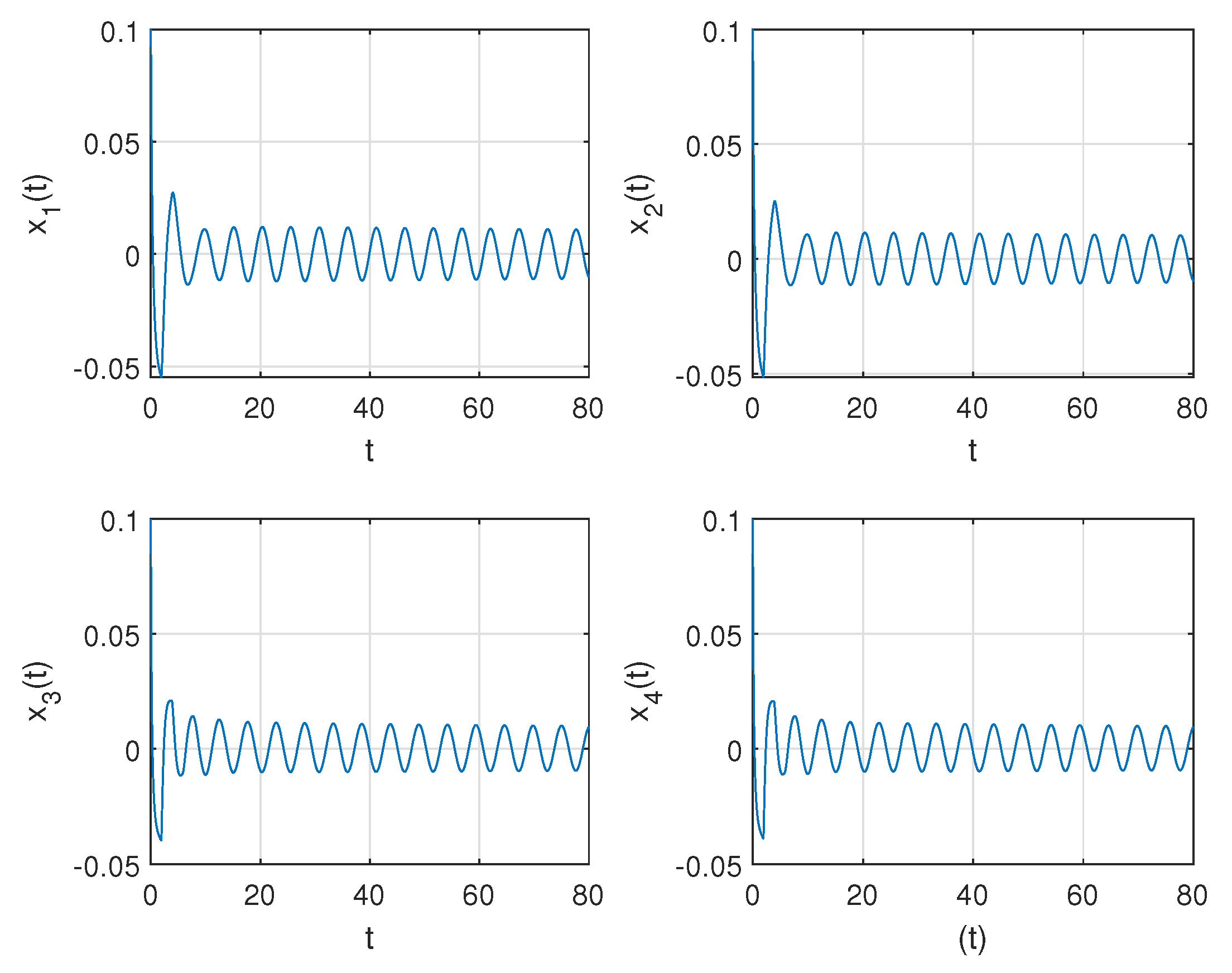
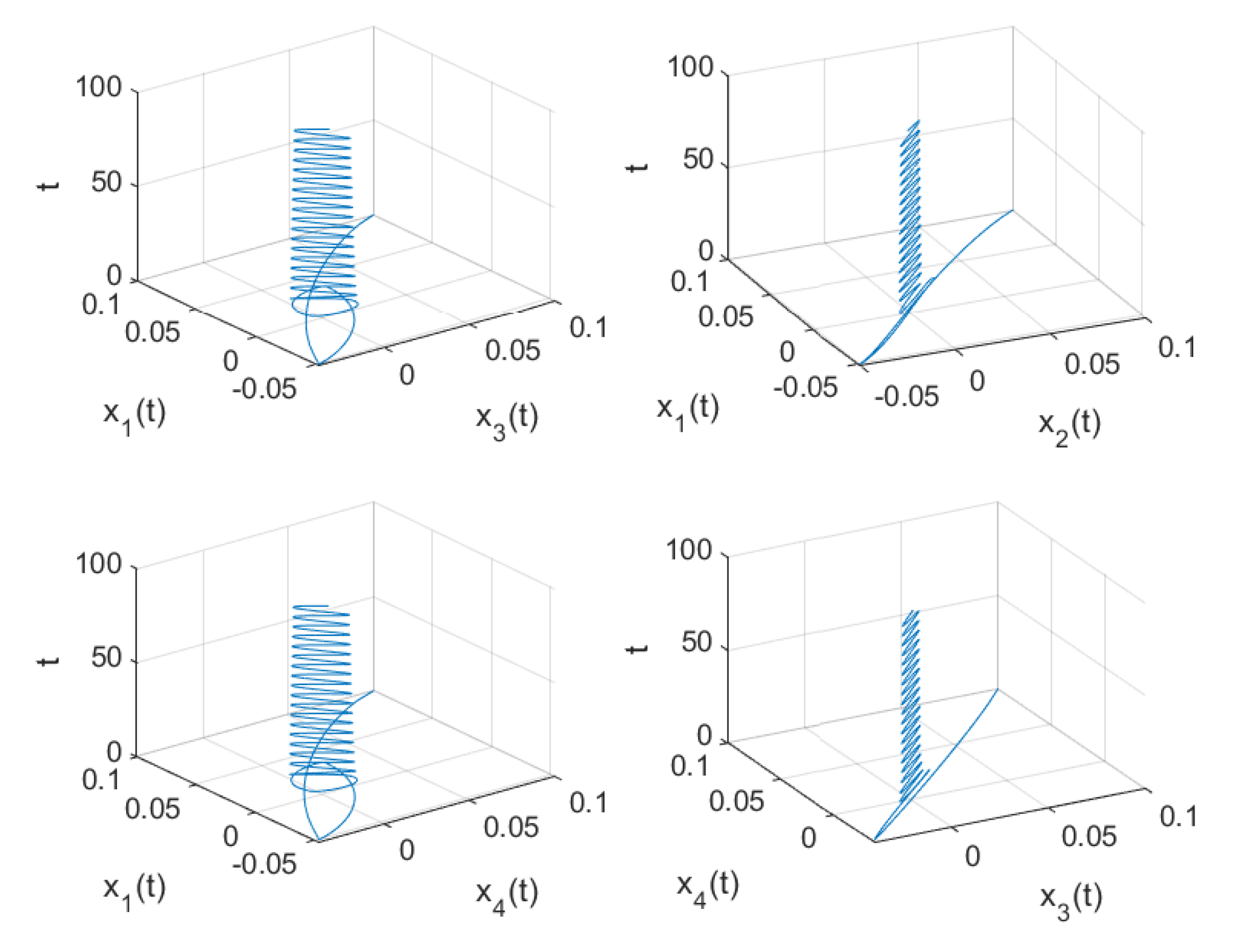
Obviously, we can see that the above system had a unique equilibrium point $E(0,0,0,0)$. We calculated ${\tau }_0=1.8885$ and ${\omega }_0=0.8069$. Figure 2 shows the waveform plots and phase diagrams of the neurons in system (53). From Figure 2, we find that the system approached a stable equilibrium point $E(0,0,0,0)$ when $\tau =1.6<{\tau }_0=1.8885$, and when $\tau =1.9>{\tau }_0=1.8885$ the system lost stability and generated bifurcation periodic solutions near the equilibrium point, as shown in Figure 3 and Figure 4. Based on the previous assumptions $\left(H1\right)$–$\left(H4\right)$, the conclusion of Theorem 1 can be confirmed.

Next, we use the control variable method to discuss the effect of orders on the Hopf bifurcation critical value of the uncontrollable system (54). When $q_i(i=1,2,3,4)$ changed, its corresponding bifurcation point ${\tau }_0$ and frequency critical value ${\omega }_0$ could be easily determined, as shown in

Table 2. The bifurcation value changing with order $q_1,q_2$.

Different Orders	Different ${\mathit{q}}_1$		Different ${\mathit{q}}_2$
	${\mathbf{\omega }}_{\mathbf{0}}$	${\mathbf{\tau }}_{\mathbf{0}}$	${\mathbf{\omega }}_{\mathbf{0}}$	${\mathbf{\tau }}_{\mathbf{0}}$
0.1	0.8012	1.9172	0.8195	1.8735
0.2	0.7779	1.9734	0.7963	1.9269
0.3	0.7615	2.0144	0.7798	1.9663
0.4	0.7519	2.0384	0.7700	1.9894
0.5	0.7491	2.0440	0.7669	1.9954
0.6	0.7527	2.0322	0.7703	1.9844
0.7	0.7627	2.0033	0.7801	1.9572
0.8	0.7789	1.9594	0.7963	1.9150
0.9	0.8015	1.9018	0.8191	1.8590
1	0.8312	1.8312	0.8493	1.7902

and

Table 3. The bifurcation value changing with order $q_3,q_4$.

Different Orders	Different ${\mathit{q}}_3$		Different ${\mathit{q}}_4$
	${\mathbf{\omega }}_{\mathbf{0}}$	${\mathbf{\tau }}_{\mathbf{0}}$	${\mathbf{\omega }}_{\mathbf{0}}$	${\mathbf{\tau }}_{\mathbf{0}}$
0.1	0.8348	1.8383	0.8377	1.8316
0.2	0.8121	1.8883	0.8152	1.8808
0.3	0.7959	1.9253	0.7991	1.9172
0.4	0.7862	1.9471	0.7895	1.9386
0.5	0.7831	1.9527	0.7864	1.9441
0.6	0.7864	1.9421	0.7898	1.9334
0.7	0.7962	1.9158	0.7996	1.9072
0.8	0.8124	1.8749	0.8158	1.8666
0.9	0.8354	1.8204	0.8389	1.8123
1	0.8660	1.7530	0.8695	1.7452

. At the same time, as shown in Figure 5, we plotted the curve of the bifurcation value changing with order. From the figure, it is evident that the bifurcation value gradually decreased and then increased as the order increased; the bifurcation value was smallest when $q_i=0.5$.

Example 2. 

In this example, we mainly considered the following controllable fractional-order system with cooperation–competition relationships:

$$\left\{\begin{array}{cc}\hfill D^{0.92}{x}_1\left(t\right)& =-x_1\left(t\right)+0.3f\left(x_1\left(t\right)\right)-1.5f\left(x_1(t-{\tau }_1)\right)\hfill \\ \hfill & +0.5(x_2\left(t\right)-x_1\left(t\right))-0.5(x_4\left(t\right)-x_1\left(t\right))\hfill \\ \hfill & -0.5(x_3\left(t\right)-x_1\left(t\right))+K_1(x_1(t-\tau )-x_1\left(t\right)),\hfill \\ \hfill D^{0.85}{x}_2\left(t\right)& =-x_2\left(t\right)+0.3f\left(x_2\left(t\right)\right)-1.5f\left(x_2(t-{\tau }_2)\right)\hfill \\ \hfill & +0.5(x_1\left(t\right)-x_2\left(t\right))-0.5(x_4\left(t\right)-x_2\left(t\right))\hfill \\ \hfill & -0.5(x_3\left(t\right)-x_2\left(t\right)),\hfill \\ \hfill D^{0.77}{x}_3\left(t\right)& =-x_3\left(t\right)+0.3f\left(x_3\left(t\right)\right)-1.5f\left(x_3(t-{\tau }_3)\right)\hfill \\ \hfill & +0.5(x_4\left(t\right)-x_3\left(t\right))-0.5(x_1\left(t\right)-x_3\left(t\right))\hfill \\ \hfill & -0.5(x_2\left(t\right)-x_3\left(t\right)),\hfill \\ \hfill D^{0.75}{x}_4\left(t\right)& =-x_4\left(t\right)+0.3f\left(x_4\left(t\right)\right)-1.5f\left(x_4(t-{\tau }_4)\right)\hfill \\ \hfill & +0.5(x_3\left(t\right)-x_4\left(t\right))-0.5(x_1\left(t\right)-x_4\left(t\right))\hfill \\ \hfill & -0.5(x_2\left(t\right)-x_4\left(t\right))+K_1(x_4(t-\tau )-x_4\left(t\right)).\hfill \end{array}\right.$$

(54)

It is obvious that system (54) had a unique equilibrium, $E_{*}(0,0,0,0)$. In order to better demonstrate the effectiveness of the bifurcation control of the delay feedback controller proposed in this article, we adopted all the parameters and orders set in Example 1. To compare with Figure 3 and Figure 4, we still took $\tau =1.9$ and the feedback gain coefficient $k_1=0.4$. We calculated that the bifurcation point ${\tau }_0=3.1056$ and the critical frequency ${\omega }_0=0.4773$. 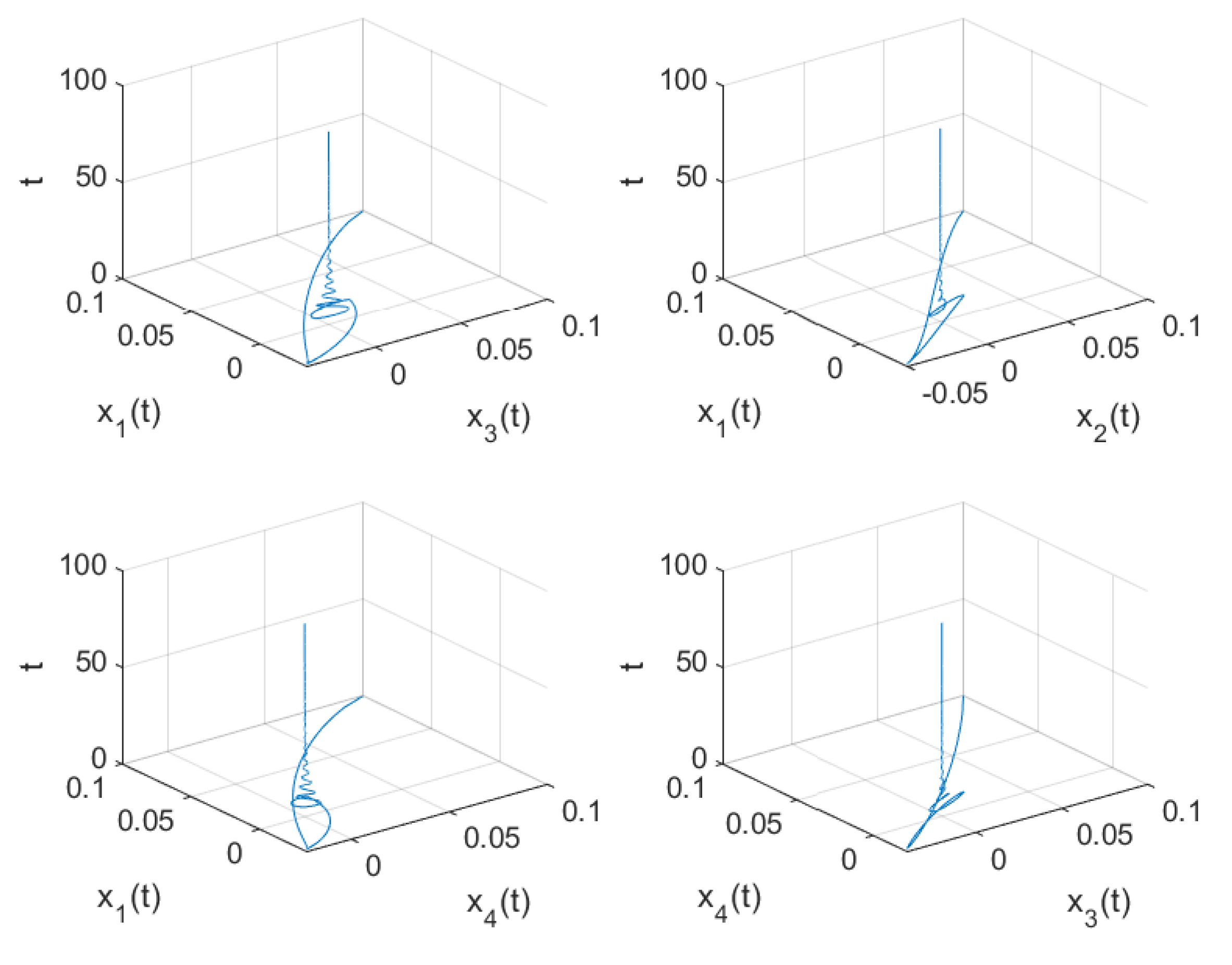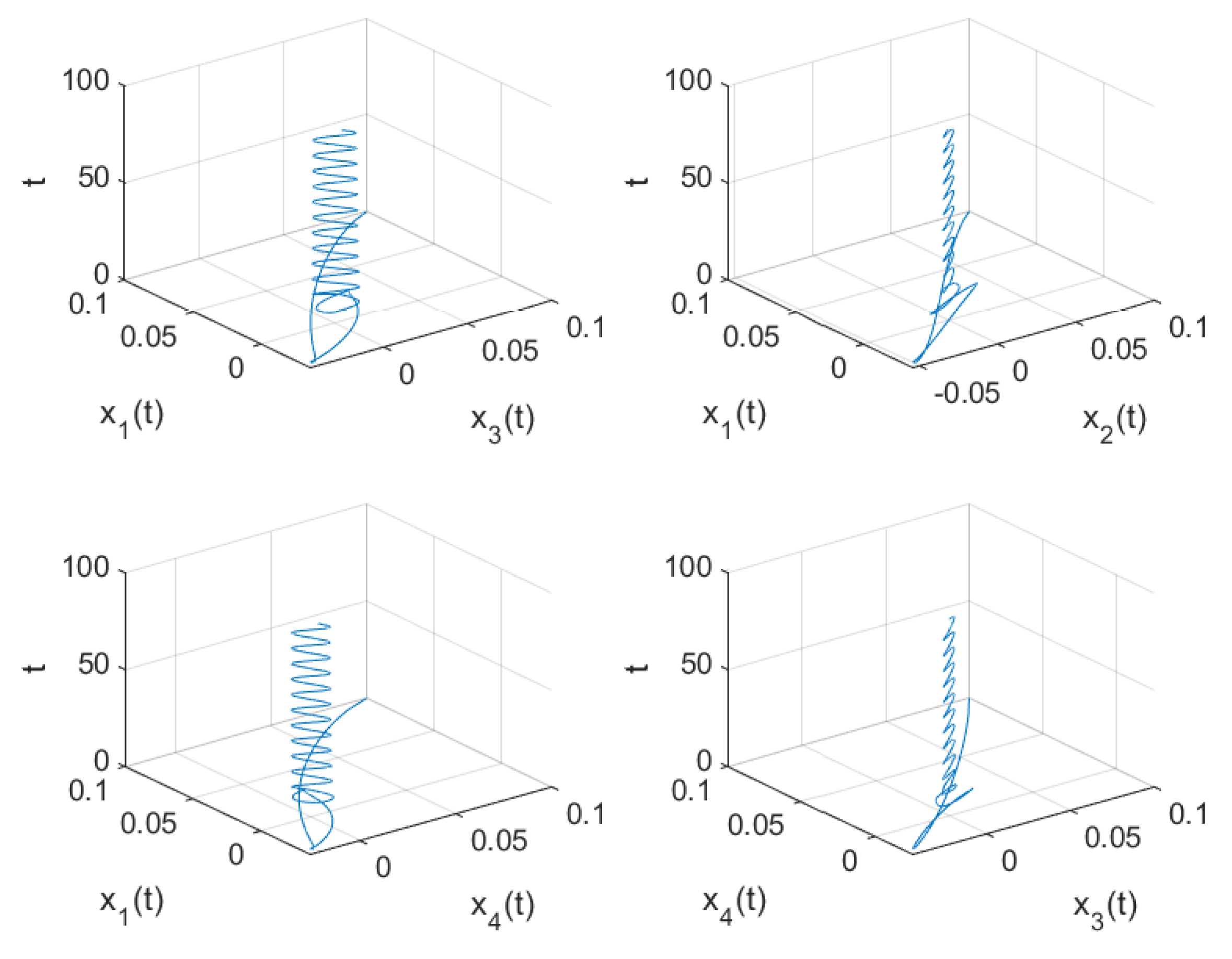Figure 5 and Figure 6 show the waveform plots and phase diagrams of the neurons in system (54). From Figure 5, we can see that the system approached a stable equilibrium point $E_{*}(0,0,0,0)$ when $\tau =1.9<{\tau }_{*}=3.1056$ and when the $\tau =3.2>{\tau }_{*}=3.1056$ the system lost stability and generated a bifurcation periodic solution near the equilibrium point, as shown in Figure 7 and Figure 8. Based on the previous assumptions $\left(H1\right)$–$\left(H2\right),\left(H5\right)$–$\left(H6\right)$, the conclusion of Theorem 2 can be confirmed.

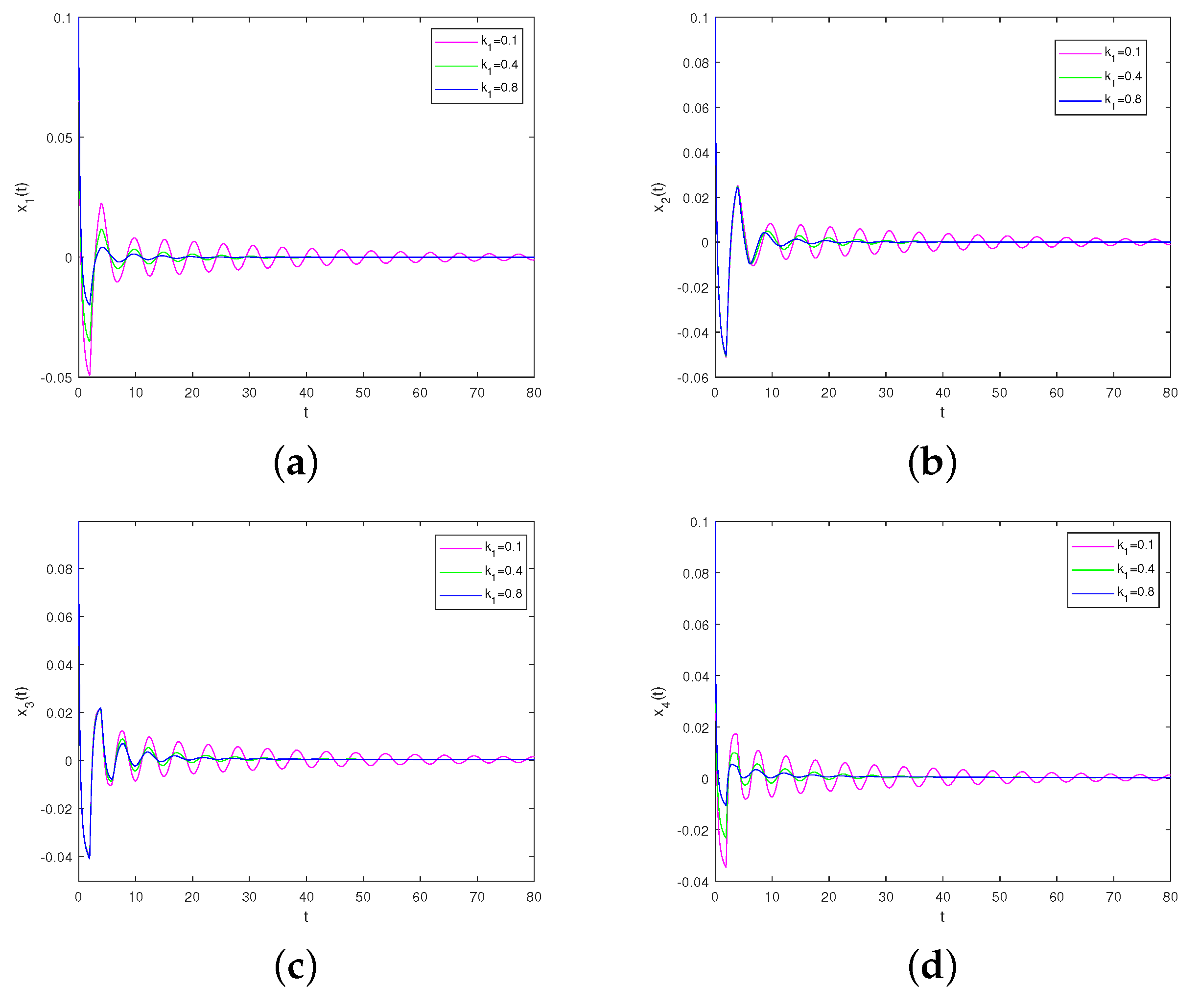
Remark 8. 

From Figure 2, it can be seen that the uncontrolled system (53) was unstable and that periodic solutions would appear when $\tau =1.9$. Figure 5 shows that at $\tau =1.9$, the controlled system (54) was locally asymptotically stable at the equilibrium point. Comparing Figure 2 with Figure 5, the results show the effectiveness of our designed delay feedback controller.

In addition, we investigated the effect of feedback gain parameter $k_1$ on the dynamic behavior of the system. Figure 9 and Figure 10 show that with the increase of $k_1$ in system (54) the bifurcation control of the controller became more pronounced.

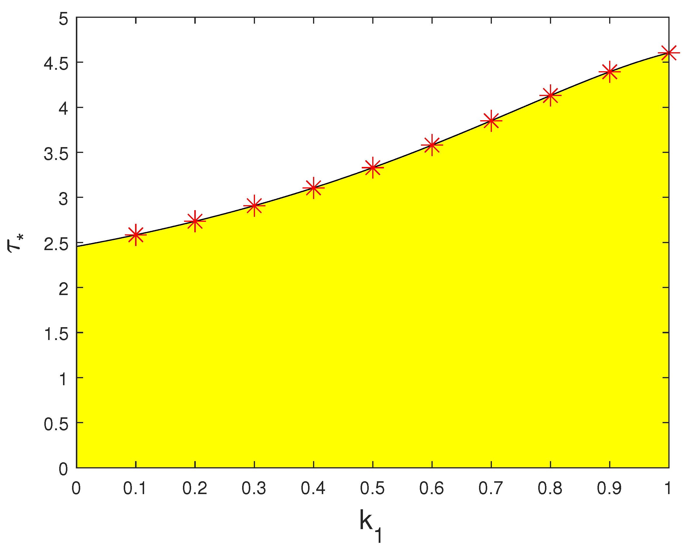
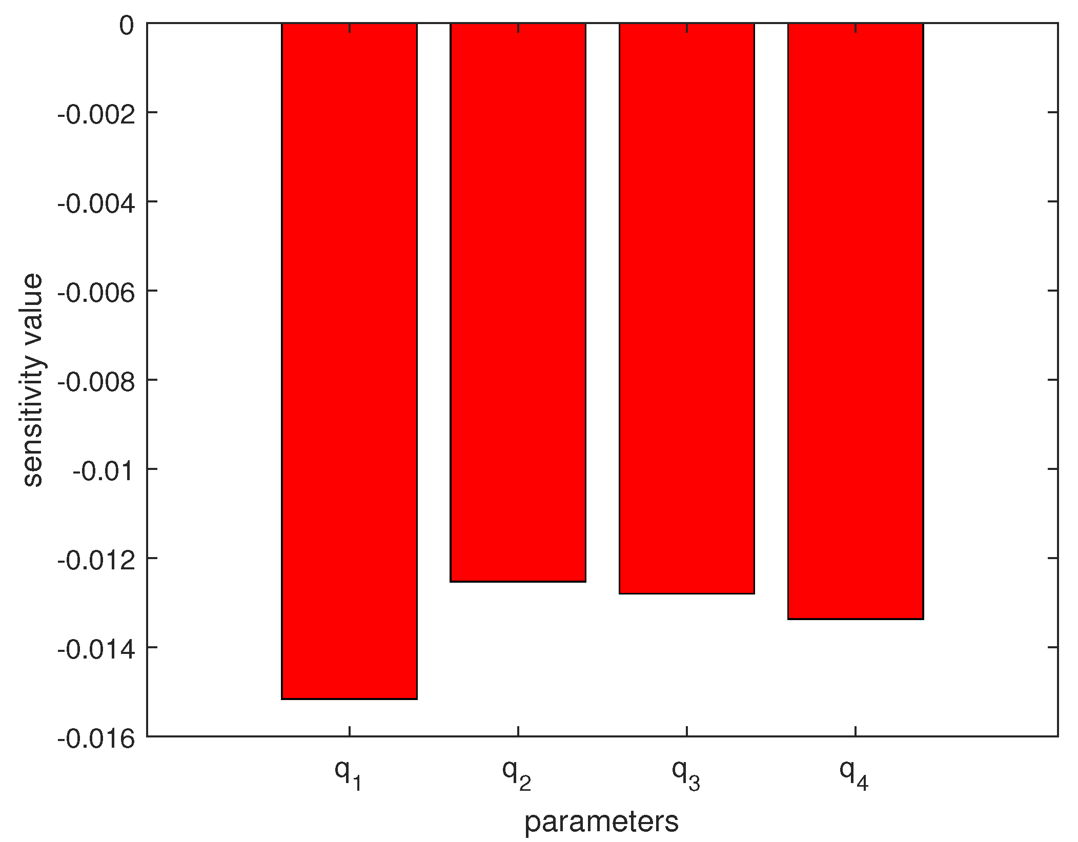
Remark 9. 

From Figure 10, it can be seen that as the feedback gain coefficient $k_1$ increases, the Hopf bifurcation value ${\tau }_{*}$ of the system increases. The yellow region is the stable region of system (54), which will undergo Hopf bifurcation on the boundary curve. When the values of $k_1$ and τ exceed the region, system (54) will bifurcate out of its periodic solution from the equilibrium point. This indicates that as the feedback gain coefficient $k_1$ increases, the start of the Hopf bifurcation can be delayed, which broadens the stability threshold of the control system, and the bifurcation control of the controller becomes more pronounced.

In order to further analyze the impact of changes in the fractional order of the system on bifurcation, we provide a sensitivity analysis of the system to order. As shown in Figure 11, $q_1$ has stronger sensitivity to the bifurcation critical value.

6. Conclusions

For this article, we investigated the bifurcation control problem of fractional-order neural networks with general cooperation–competition topology. Our research mainly focused on the following aspects. Firstly, self-feedback delay was selected as the bifurcation parameter to analyze the bifurcation dynamic behavior of the uncontrolled system, and a new sufficient condition was established to ensure the stability of the network model and the existence of Hopf bifurcation. Secondly, the influence of fractional order on the bifurcation critical value of uncontrolled systems was discussed. Then, a time-delay feedback controller was introduced to study the stability of its controlled system and the existence of Hopf bifurcation. Finally, the influence of feedback gain coefficient on the controlled system was discussed. The results indicate that when $q_i(i=1,2,3,4)\in (0,0.5)$, reducing the order will delay the start of Hopf bifurcation and broaden its stability threshold. When $q_i(i=1,2,3,4)\in (0.5,1)$, reducing the order will delay the start of Hopf bifurcation and broaden its stability threshold. In addition, for uncontrolled systems, increasing the feedback gain coefficient $k_1$ results in more pronounced bifurcation control of the controller.

In future research, we will introduce more types of controllers to broaden the stability thresholds of network models.