On the Visibility of Homogeneous Cantor Sets

Abstract

The problems associated with the visible set have been explored by various scholars. In this paper, we investigate the Hausdorff dimension and the topological properties of the visible set in relation to the products of homogeneous Cantor sets. To address these issues and establish our results, we employ beta expansion theory, numerical calculations and several technical results from fractal geometry. Our research reveals that the case of the homogeneous Cantor set differs from those of the middle Cantor sets. Furthermore, we identify a critical number that is linked to both the Hausdorff dimension and the topological properties of the visible set.

1. Introduction

Given $m\ge 1$ and $\beta \in \left(0,{\displaystyle \frac{1}{m+1}}\right)$, let ${\mathsf{\Gamma }}_{\beta ,m}\subset \mathbb{R}$ be the set generated by the iterated function system (see [1]) below:

$$\left\{f_i\left(x\right)=\beta x+{\displaystyle \frac{i(1-\beta )}{m}};i=0,1,\cdots ,m\right\}$$

i.e., ${\mathsf{\Gamma }}_{\beta ,m}$ is the unique nonempty compact set satisfying

$${\mathsf{\Gamma }}_{\beta ,m}=\bigcup _{i=0}^m{f}_i\left({\mathsf{\Gamma }}_{\beta ,m}\right).$$

(1)

The set ${\mathsf{\Gamma }}_{\beta ,m}$ is the homogeneous Cantor set; in particular, ${\mathsf{\Gamma }}_{\beta ,1}$ represents the middle-$(1-2\beta )$ Cantor set, while ${\mathsf{\Gamma }}_{1/3,1}$ corresponds to the classical middle third Cantor set. The middle-$(1-2\beta )$ Cantor sets have been extensively studied in the past, with research focusing on topics such as the structure and dimension of intersections of Cantor sets [2,3] and the arithmetic properties of Cantor sets [4,5,6]. Subsequent studies have extended the investigation to more general cases of homogeneous Cantor sets [7,8,9,10].

Given $0<\alpha \in \mathbb{R}$ and the subset $F\subset {\mathbb{R}}^2$, we say the line $y=\alpha x$ is visible through F if

$$\left\{\right(x,\alpha x):x\ne 0\}\cap F=\varnothing .$$

The issue of visibility arising from various works, e.g., Orponen [11], provided an upper bound on the Hausdorff dimension of the visible parts of a compact set. Järvenpää et al. [12] established an upper bound for the Assouad dimension of the visible parts of self-similar sets generated by iterated function systems with finite rotation groups and satisfying the weak separation condition. Additionally, Zhang et al. [13] offered a characterization of visibility concerning the products of the middle-$(1-2\beta )$ Cantor sets. For further information, we refer readers to [14,15] and the references therein.

In [13], the authors investigate the visible set on the middle Cantor set, analyzing its Hausdorff dimension and topological structure. In this case, the middle Cantor set is generated by an iterated function system (IFS) consisting of only two contraction functions. However, when the middle Cantor set is replaced by a homogeneous Cantor set, the IFS becomes significantly more complex. Therefore, in this paper, we explore the Hausdorff dimension and topological properties of the visible set with respect to the product of homogeneous Cantor set. More precisely, we are interested in the visible set shown below:

$$V:=\left\{\alpha >0:\{(x,\alpha x):x\ne 0\}\cap \left({\mathsf{\Gamma }}_{\beta ,m}\times {\mathsf{\Gamma }}_{\beta ,m}\right)=\varnothing \right\}.$$

Clearly, $\alpha \in V$ is equivalent to

$$\alpha \notin \mathsf{\Lambda }:=\left\{{\displaystyle \frac{x}{y}}:x,y\in {\mathsf{\Gamma }}_{\beta ,m},y\ne 0\right\}=[0,\infty )\setminus V.$$

Main Results

Since the case $m=1$ has been proven in [13], we focus on the case $m>1$ in this study. Let

$$f_m\left(\beta \right):={\beta }^2-(m^2+2)\beta +1.$$

(2)

Denote by ${\beta }_m$ the smallest positive root of $f_m\left(\beta \right)$. Now, we state our results:

Theorem 1. 

Given $m>1$ and $\beta \in \left(0,{\displaystyle \frac{1}{m+1}}\right)$

(i) 

If ${\displaystyle \frac{1}{2m+1}}\le \beta <{\displaystyle \frac{1}{m+1}}$, then $V=\varnothing$.

(ii) 

If $0<\beta <{\beta }_m$, where ${\beta }_m$ is the smallest positive root of (2), then V has an interior point.

(iii) 

If $0<\beta \le {\displaystyle \frac{1}{{(m+1)}^2}}$, Λ has Lebesgue measure zero and ${dim}_H\left(\mathsf{\Lambda }\right)={\displaystyle \frac{2log(m+1)}{-log\beta }}$.

The paper is arranged as follows. In Section 2, we give the proof of Theorem 1. Finally, we conclude our study in Section 3.

2. Proof of Theorem 1

It is well known that ${\mathsf{\Gamma }}_{\beta ,m}$ can be obtained from the interval $[0,1]$ by removing m fixed proportions of each subinterval in each step. We denote by $I_n$ the union of all the basic intervals of rank n and let $I^{\prime }={\cup }_{i=0}^m{f}_i\left(I\right)$, where I is a basic interval.

2.1. Proof of Theorem 1(i)

The work presented in [13] (see also [16]) provides a technical result applicable to the case when $m=1$ in the following lemma. Since the proof is independent of the parameter m, this lemma holds for $m\ge 1$.

Lemma 1. 

Let $F:U\to \mathbb{R}$ be a continuous function, where $U\subset {\mathbb{R}}^2$ is a nonempty open set. Suppose A and B are the left and right endpoints of some basic intervals in $I_{k_0}$ for some $k_0\ge 1$, respectively, such that $[A,B]\times [A,B]\subset U$. Then, ${\mathsf{\Gamma }}_{\beta ,m}\cap [A,B]={\bigcap }_{n=k_0}^{\infty }{I}_n$. Moreover, if for any $n\ge k_0$ and any two basic intervals $I,J\subset I_n$,

$$F(I,J)=F(I^{\prime },J^{\prime })$$

where $F(I,J):=\left\{F\right(x,y):x\in I,y\in J\}$, then

$$F\left({\mathsf{\Gamma }}_{\beta ,m}\cap [A,B],{\mathsf{\Gamma }}_{\beta ,m}\cap [A,B]\right)=F\left(I_{k_0},I_{k_0}\right).$$

Lemma 2. 

Given $m>1$, let $g(x,y)={\displaystyle \frac{x}{y}}$, $I=[a,a+t]$ and $J=[b,b+t]$ be two basic intervals. If ${\displaystyle \frac{1}{2m+1}}\le \beta <{\displaystyle \frac{1}{m+1}}$ and $b\ge a\ge {\displaystyle \frac{1-\beta }{m}}$, then $g(I^{\prime },J^{\prime })=g(I,J)$.

Proof. 

Note that $a+t\le b+t\le 1$ and $t\le \beta$, because $I,J$ are two basic intervals. It can be verified that $g(I,J)=[{\displaystyle \frac{a}{b+t}},{\displaystyle \frac{a+t}{b}}]$ and

$$\begin{array}{cc}\hfill & I^{\prime }=\bigcup _{i=0}^m\left[a+{\displaystyle \frac{i(1-\beta )t}{m}},a+{\displaystyle \frac{i(1-\beta )t+m\beta t}{m}}\right],\hfill \\ \hfill & J^{\prime }=\bigcup _{i=0}^m\left[b+{\displaystyle \frac{j(1-\beta )t}{m}},b+{\displaystyle \frac{j(1-\beta )t+m\beta t}{m}}\right].\hfill \end{array}$$

Through this calculation, we obtain $g(I^{\prime },J^{\prime })={\cup }_{i=0}^m{\cup }_{j=0}^m[{\ell }_{i,j},r_{i,j}]$, where

$$\begin{array}{c}\hfill \left[{\displaystyle \frac{i(1-\beta )t+ma}{j(1-\beta )t+m\beta t+mb}},{\displaystyle \frac{i(1-\beta )t+m\beta t+ma}{j(1-\beta )t+mb}}\right]:=[{\ell }_{i,j},r_{i,j}],\end{array}$$

and $g(I,J)=[{\ell }_{0,m},r_{m,0}]$. We observe that for each fixed $0\le i\le m$, the sequences ${\left({\ell }_{i,j}\right)}_{i=0}^m$ and ${\left(r_{i,j}\right)}_{i=0}^m$ are decreasing, while for each fixed $0\le j\le m$, the sequences ${\left({\ell }_{i,j}\right)}_{i=0}^m$ and ${\left(r_{i,j}\right)}_{i=0}^m$ are increasing. It suffices to prove that $g(I^{\prime },J^{\prime })=[{\ell }_{0,m},r_{m,0}]$. We split the proof into two cases.

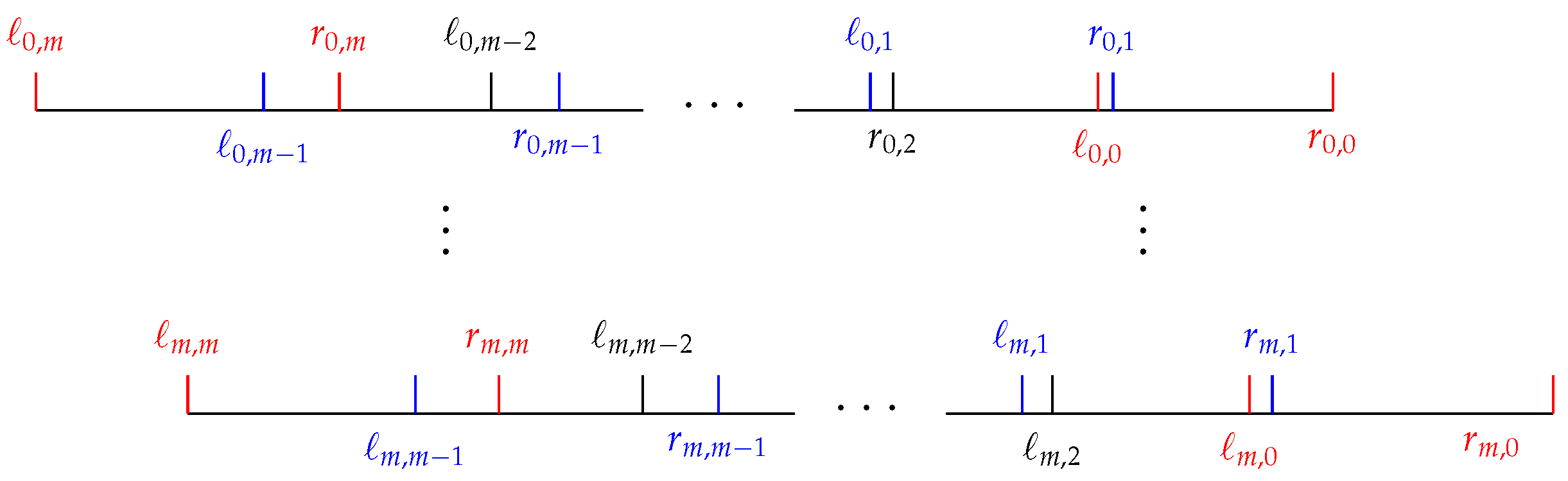
Case I. If $a\ne b$, then $b>a+t$. We will prove that the following inequalities hold:

$$r_{i,j}>{\ell }_{i,j-1},0\le i\le m\mathrm{and}1\le j\le m$$

and

$$r_{i,0}>{\ell }_{i+1,m},0\le i\le m-1.$$

For convenience, we depict the intervals $[{\ell }_{i,j},r_{i,j}]$ in Figure 1.

Firstly,

$$\begin{array}{c}\hfill r_{i,j}-{\ell }_{i,j-1}={\displaystyle \frac{i(1-\beta )t+m\beta t+ma}{j(1-\beta )t+mb}}-{\displaystyle \frac{i(1-\beta )t+ma}{(j-1)(1-\beta )t+m\beta t+mb}},\end{array}$$

where the denominator of $r_{i,j}-{\ell }_{i,j-1}$ is positive and the numerator is

$$\begin{array}{cc}\hfill & \left[i\right(1-\beta )t+m\beta t+ma]\left[\right(j-1\left)\right(1-\beta )t+m\beta t+mb]\hfill \\ \hfill -& \left[i\right(1-\beta )t+ma]\left[j\right(1-\beta )t+mb]\hfill \\ \hfill =& i{t}^2[\beta (m+1)-1]+\beta t^2(m-i)[\beta (m+1)-1]+mat[\beta (m+1)-1]\hfill \\ \hfill =& t^2[\beta (m+1)-1](i(1-\beta )+\beta m)+mat[\beta (m+1)-1]\hfill \\ \hfill +& \beta bt{m}^2+jm\beta t^2(1-\beta )\hfill \\ \hfill >& m{t}^2[\beta (m+1)-1]+mat[\beta (m+1)-1]+\beta bt{m}^2+jm\beta t^2(1-\beta )\hfill \\ \hfill >& mt\left[\right(\beta (2m+1)-1\left)\right(a+t)+j\beta t(1-\beta \left)\right]\ge 0.\hfill \end{array}$$

So, $r_{i,j}>{\ell }_{i,j-1}$. Then, we have

$${\cup }_{j=0}^m[{\ell }_{i,j},r_{i,j}]=[{\ell }_{i,m},r_{i,0}]\mathrm{for}\mathrm{any}0\le i\le m.$$

(3)

Next, we prove that for any $0\le i\le m-1$ we have $r_{i,0}>{\ell }_{i+1,m}$.

$$\begin{array}{c}\hfill r_{i,0}-{\ell }_{i+1,m}={\displaystyle \frac{it+\beta t(m-i)+ma}{mb}}-{\displaystyle \frac{t(i+1)(1-\beta )+ma}{mt+mb}},\end{array}$$

where the numerator of $r_{i,0}-{\ell }_{i+1,m}$ is

$$\begin{array}{cc}\hfill & \left[\right(it+\beta t(m-i)+ma\left)\right](mt+mb)-mb\left[t\right(i+1\left)\right(1-\beta )+ma]\hfill \\ \hfill =& im{t}^2+\beta m{t}^2(m-i)+at{m}^2+\beta bt{m}^2+\beta mbt-mbt\hfill \\ \hfill =& mt[it+\beta t(m-i)+am+\beta mb+\beta b-b]\hfill \\ \hfill \ge & mt[\beta mt+am+\beta b(m+1)-b]\hfill \\ \hfill >& mt[\beta mt+1-\beta +\beta (m+1)-1]>0.\hfill \end{array}$$

The penultimate inequality follows from $a\ge {\displaystyle \frac{1-\beta }{m}}$ and $b<1$. Together with (3), we hence deduce that $g(I^{\prime },J^{\prime })={\cup }_{i=0}^m{\cup }_{j=0}^m[{\ell }_{i,j},r_{i,j}]=[{\ell }_{0,m},r_{m,0}]$.

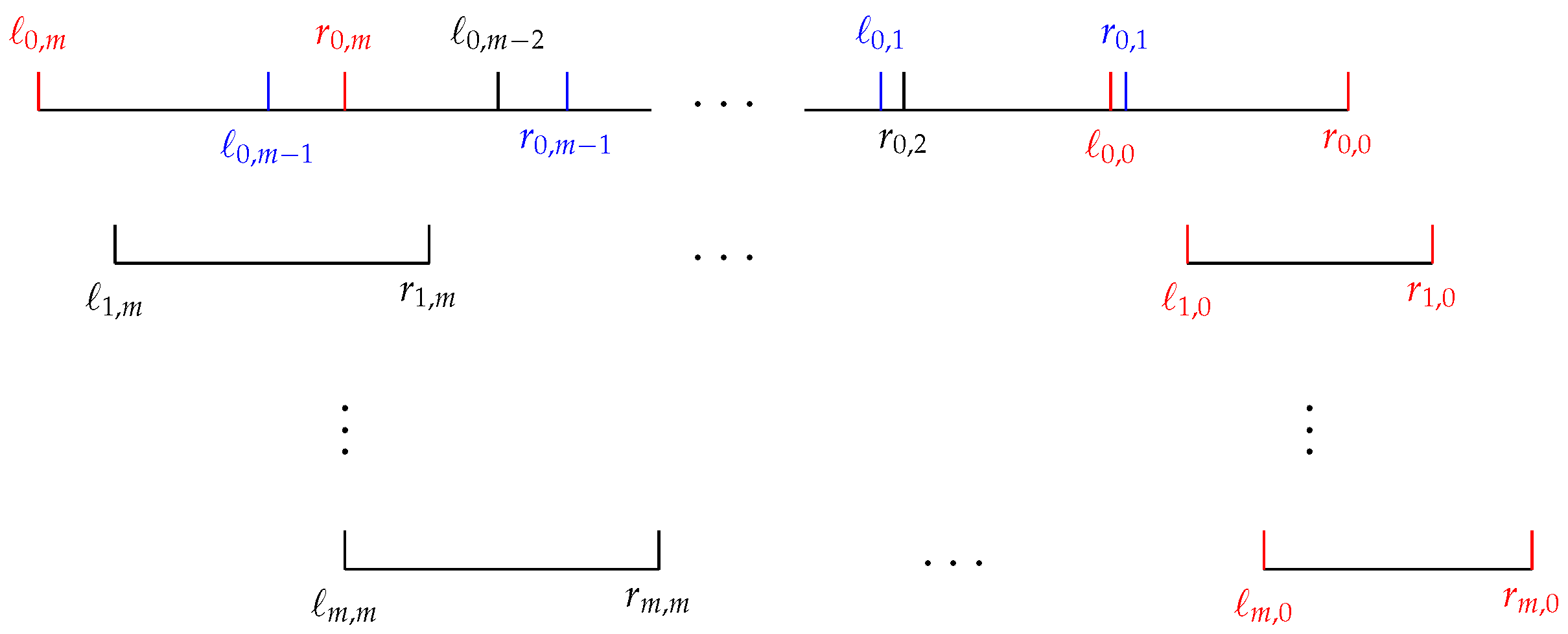
Case II. If $a=b$. This case is illustrated in Figure 2, and we prove that

$$r_{0,j}>{\ell }_{0,j-1},1\le j\le m\mathrm{and}{r}_{i,0}>{\ell }_{i+1,0},0\le i\le m-1.$$

Firstly, for any $1\le j\le m$

$$\begin{array}{c}\hfill r_{0,j}-{\ell }_{0,j-1}={\displaystyle \frac{m\beta t+ma}{j(1-\beta )t+mb}}-{\displaystyle \frac{ma}{(j-1)(1-\beta )t+m\beta t+mb}}.\end{array}$$

Using the calculation in Case I, the numerator of $r_{0,j}-{\ell }_{0,j-1}$ is

$$\begin{array}{cc}\hfill & mt\left[\right(\beta (m+1)-1\left)\right(a+\beta t)+\beta ma+j\beta t(1-\beta \left)\right]\hfill \\ \hfill \ge & mt\left[\right[\beta (2m+1)-1]a+\beta t(\beta m+\beta -1+1-\beta \left)\right]>0.\hfill \end{array}$$

So, we have $r_{0,j}>{\ell }_{0,j-1}$. Finally, for any $0\le i\le m-1$

$$\begin{array}{c}\hfill r_{i,0}-{\ell }_{i+1,0}={\displaystyle \frac{it+\beta t(m-i)+ma}{mb}}-{\displaystyle \frac{t(i+1)(1-\beta )+ma}{m\beta t+mb}},\end{array}$$

the numerator of $r_{i,0}-{\ell }_{i+1,0}$ is

$$\begin{array}{cc}\hfill & \left[\right(it+\beta t(m-i)+ma\left)\right](m\beta t+ma)-ma\left[t\right(i+1\left)\right(1-\beta )+ma]\hfill \\ \hfill =& im\beta t^2+m{\beta }^2{t}^2(m-i)+a\beta t{m}^2+\beta at{m}^2+\beta mat-mat\hfill \\ \hfill =& mt[i\beta t+t(m-i){\beta }^2+am\beta +am\beta +\beta a-a]\hfill \\ \hfill \ge & mt[mt{\beta }^2+\beta a(2m+1)-a]>0.\hfill \end{array}$$

The final inequality follows from $t\le \beta$, thus completing the proof. □

Lemma 3. 

Let $m>1$ and ${\displaystyle \frac{1}{2m+1}}\le \beta <{\displaystyle \frac{1}{m+1}}$. Then, $\mathsf{\Lambda }=[0,\infty )$.

Proof. 

We begin by observing that each $x\in {\mathsf{\Gamma }}_{\beta ,m}$ can be written as

$$x={\displaystyle \frac{1-\beta }{m\beta }}\sum _{n=1}^{\infty }{x}_n{\beta }^n,x_n\in \{0,1,\cdots ,m\}$$

and $y\in {\cup }_{i=1}^m{f}_i\left({\mathsf{\Gamma }}_{\beta ,m}\right)$ can be written as

$$y={\displaystyle \frac{1-\beta }{m\beta }}\sum _{n=1}^{\infty }{y}_n{\beta }^n,$$

where $y_1\in \{1,\cdots ,m\}$ and $y_n\in \{0,1,\cdots ,m\}$ for $n\ge 2$. So, for any $x\in {\mathsf{\Gamma }}_{\beta ,m}\setminus \left\{0\right\}$, we have

$$x={\beta }^{n}y,n\in \mathbb{N}.$$

On the other hand, if ${\displaystyle \frac{1}{2m+1}}\le \beta <{\displaystyle \frac{1}{m+1}}$, then by Lemmas 1 and 2 for $0<i,j\le m$, we have

$${\displaystyle \frac{f_i\left({\mathsf{\Gamma }}_{\beta ,m}\right)}{f_j\left({\mathsf{\Gamma }}_{\beta ,m}\right)}}=\left[{\displaystyle \frac{i(1-\beta )}{j(1-\beta )+m\beta }},{\displaystyle \frac{i(1-\beta )+m\beta }{j(1-\beta )}}\right]:=[p_{i,j},q_{i,j}].$$

Now, we show that $p_{i+1,1}<q_{i,1}$ and $p_{1,j}<q_{1,j+1}$. We apply the same method as in Case II of the proof for Lemma 2:

$$\begin{array}{c}\hfill q_{i,1}-p_{i+1,1}={\displaystyle \frac{i(1-\beta )+m\beta }{1-\beta }}-{\displaystyle \frac{(i+1)(1-\beta )}{1-\beta +m\beta }},\end{array}$$

the numerator of $q_{i,1}-p_{i+1,1}$ is

$$\begin{array}{cc}\hfill & [i(1-\beta )+m\beta ](1-\beta +m\beta )-(i+1){(1-\beta )}^2\hfill \\ \hfill =& im\beta (1-\beta )+m\beta (1-\beta )+m^2{\beta }^2-{(1-\beta )}^2\hfill \\ \hfill >& (1-\beta )\left[\right(2m+1)\beta -1]\ge 0.\hfill \end{array}$$

Secondly,

$$p_{1,j}-q_{1,j+1}={\displaystyle \frac{1-\beta }{j(1-\beta )+m\beta }}-{\displaystyle \frac{1-\beta +m\beta }{(j+1)(1-\beta )}},$$

the numerator of $p_{1,j}-q_{1,j+1}$ is

$$\begin{array}{cc}\hfill & (j+1){(1-\beta )}^2-(1-\beta +m\beta )[j(1-\beta )+m\beta ]\hfill \\ \hfill =& {(1-\beta )}^2-m\beta (1-\beta )-jm\beta (1-\beta )-m^2{\beta }^2\hfill \\ \hfill <& (1-\beta )[1-(2m+1\left)\beta \right]\le 0.\hfill \end{array}$$

Based on the above reasoning, we see that ${\cup }_{i,j=1}^m{\displaystyle \frac{f_i\left({\mathsf{\Gamma }}_{\beta ,m}\right)}{f_j\left({\mathsf{\Gamma }}_{\beta ,m}\right)}}=[p_{1,m},q_{m,1}]=[{\displaystyle \frac{1-\beta }{m}},{\displaystyle \frac{m}{1-\beta }}]$. Thus, for $x_1={\beta }^{n_1}{y}_1,x_2={\beta }^{n_2}{y}_2\in {\mathsf{\Gamma }}_{\beta ,m}\setminus \left\{0\right\}$ with $n_1,n_2\in \mathbb{N}$ and $y_1,y_2\in {\cup }_{i=1}^m{f}_i\left({\mathsf{\Gamma }}_{\beta ,m}\right)$, we have

$${\displaystyle \frac{x_1}{x_2}}={\beta }^{n_1-n_2}·{\displaystyle \frac{y_1}{y_2}}.$$

So, this in turn implies

$$\mathsf{\Lambda }=\left\{0\right\}\cup \bigcup _{n=-\infty }^{\infty }{\beta }^n\left[{\displaystyle \frac{1-\beta }{m}},{\displaystyle \frac{m}{1-\beta }}\right].$$

Let ${\beta }^n[{\displaystyle \frac{1-\beta }{m}},{\displaystyle \frac{m}{1-\beta }}]:=[A_n,B_n]$. The numerator of $A_n-B_{n+1}$ is

$${\beta }^n[{\beta }^2-(m^2+2)\beta +1]={\beta }^n{f}_m\left(\beta \right)$$

where $f_m\left(\beta \right)$ is defined in (2). It can be verified that $f_m\left(\beta \right)$ is strictly decreasing for $\beta <1$ and ${\beta }_m<{\displaystyle \frac{1}{2m+1}}$ when $m>1$. Hence, the intervals $[A_n,B_n]$ are pairwise disjoint when $0<\beta <{\beta }_m$. In other words, if $m>1$, we have ${\bigcup }_{n=-\infty }^{\infty }[A_n,B_n]=(0,\infty )$ for all ${\displaystyle \frac{1}{2m+1}}\le \beta <{\displaystyle \frac{1}{m+1}}$. Thus, the proof is complete. □

Proof of Theorem 1(i). Using Lemma 3, we see when ${\displaystyle \frac{1}{2m+1}}\le \beta <{\displaystyle \frac{1}{m+1}},V=[0,\infty )\setminus \mathsf{\Lambda }=\varnothing$.

2.2. Proof of Theorem 1(ii)

Lemma 4. 

Let $m>1$, and let ${\beta }_m$ be defined as in (2). If $0<\beta <{\beta }_m$, then V has an interior point.

Proof. 

We observe that the intervals $[A_n,B_n]$ are pairwise disjointed for $0<\beta <{\beta }_m$. Using the proof of Lemma 3, we have

$$\mathsf{\Lambda }\subseteq \left\{0\right\}\cup \bigcup _{n=-\infty }^{\infty }[A_n,B_n].$$

Therefore, $(0,\infty )\setminus {\bigcup }_{n=-\infty }^{\infty }[A_n,B_n]$ contains interior point and so

$$(0,\infty )\setminus \bigcup _{n=-\infty }^{\infty }[A_n,B_n]\subset V=[0,\infty )\setminus \mathsf{\Lambda }$$

has an interior point. □

Proof of Theorem 1(ii). We can draw a conclusion via Lemma 4.

2.3. Proof of Theorem 1(iii)

In what follows, we pay attention to the measure and dimension. First, we present two important results as follows:

Proposition 1 

([17]). Let S be a self-similar 1-set in ${\mathbb{R}}^2$ with the open set condition, which is not on a line. Then, the Lebesgue measure of $P_{(0,0)}(S\setminus \left\{(0,0)\right\})$ is zero, where

$$P_{(0,0)}(x,y)={\displaystyle \frac{(x,y)}{\sqrt{x^2+y^2}}}.$$

Proposition 2 

([18]). Let S be an arbitrary self-similar set in ${\mathbb{R}}^2$ not contained in any line. Suppose that $g:{\mathbb{R}}^2\to \mathbb{R}$ is a $C^2$ map such that for any $(x,y)\in S$

$$\begin{array}{c}\hfill \begin{array}{cc}\hfill & {\left(g_x\right)}^2+{\left(g_y\right)}^2\ne 0\hfill \\ \hfill & {(g_{xx}{g}_y-g_{xy}{g}_x)}^2+{(g_{xy}{g}_y-g_{yy}{g}_x)}^2\ne 0.\hfill \end{array}\end{array}$$

(4)

Then

$${dim}_{H}g\left(S\right)=min\left\{1,{dim}_H\left(S\right)\right\}.$$

In the following, let $m>1$, and we use ${\mathsf{\Gamma }}_{\beta }$ instead of ${\mathsf{\Gamma }}_{\beta ,m}$ for brevity.

Lemma 5. 

If $\beta ={\displaystyle \frac{1}{{(m+1)}^2}}$, then Λ has a Lebesgue measure of zero.

Proof. 

Let $\beta ={\displaystyle \frac{1}{{(m+1)}^2}}$, where the IFS satisfies open set condition and ${\mathsf{\Gamma }}_{\beta }\times {\mathsf{\Gamma }}_{\beta }$ is a self-similar 1-set(see [1]). Setting

$$S_1=\left\{{\displaystyle \frac{(x,y)}{\sqrt{x^2+y^2}}}:(x,y)\in {\mathsf{\Gamma }}_{\beta }\times {\mathsf{\Gamma }}_{\beta },x\ne 0\right\}$$

and

$$S_2=\left\{arctan{\displaystyle \frac{y}{x}}:(x,y)\in {\mathsf{\Gamma }}_{\beta }\times {\mathsf{\Gamma }}_{\beta },x\ne 0\right\}.$$

We can build a Lipschitz map between $S_1$ and $S_2$ as follows:

$$\mathrm{\Phi }\left({\displaystyle \frac{(x,y)}{\sqrt{x^2+y^2}}}\right)=arctan{\displaystyle \frac{y}{x}}.$$

It follows from Proposition 1 that $S_1$ has a Lebesgue measure of zero. Furthermore, since $\mathsf{\Phi }$ is Lipschitz, it follows that $S_2$ and, subsequently, $\mathsf{\Lambda }$ both have a Lebesgue measure of zero. □

Lemma 6. 

When $0<\beta \le {\displaystyle \frac{1}{{(m+1)}^2}}$, then ${dim}_H\left(\mathsf{\Lambda }\right)={\displaystyle \frac{2log(m+1)}{-log\beta }}$.

Proof. 

Since

$$\mathsf{\Lambda }\subseteq \left\{0\right\}\cup \bigcup _{n=-\infty }^{\infty }\bigcup _{i,j=1}^m{\beta }^n{\displaystyle \frac{f_i\left({\mathsf{\Gamma }}_{\beta ,m}\right)}{f_j\left({\mathsf{\Gamma }}_{\beta ,m}\right)}},$$

by the stability of the Hausdorff dimension, we have

$${dim}_H\mathsf{\Lambda }=max\left\{{dim}_H{\displaystyle \frac{f_i\left({\mathsf{\Gamma }}_{\beta }\right)}{f_j\left({\mathsf{\Gamma }}_{\beta }\right)}}:1\le i,j\le m\right\}.$$

On the other hand, $T(x,y)={\displaystyle \frac{x}{y}}$ satisfies (4) for any $(x,y)\in S_{i,j}=f_i\left({\mathsf{\Gamma }}_{\beta }\right)\times f_j\left({\mathsf{\Gamma }}_{\beta }\right)$, by Proposition 2

$$\begin{array}{cc}\hfill {dim}_{H}T\left(S_{i,j}\right)& ={dim}_H{\displaystyle \frac{f_i\left({\mathsf{\Gamma }}_{\beta }\right)}{f_j\left({\mathsf{\Gamma }}_{\beta }\right)}}\hfill \\ \hfill & =min\left\{{dim}_H\left(S_{i,j}\right),1\right\}\hfill \\ \hfill & =min\left\{2{dim}_H\left({\mathsf{\Gamma }}_{\beta }\right),1\right\}.\hfill \end{array}$$

The last equality follows from ${dim}_H\left(f_k\left({\mathsf{\Gamma }}_{\beta }\right)\right)={dim}_B\left(f_k\left({\mathsf{\Gamma }}_{\beta }\right)\right)={dim}_H\left({\mathsf{\Gamma }}_{\beta }\right)={\displaystyle \frac{2log(m+1)}{-log\beta }},1\le k\le m$. Therefore, when $0<\beta \le {\displaystyle \frac{1}{{(m+1)}^2}}$, we obtain

$${dim}_H{\displaystyle \frac{f_i\left({\mathsf{\Gamma }}_{\beta }\right)}{f_j\left({\mathsf{\Gamma }}_{\beta }\right)}}=2{dim}_H\left({\mathsf{\Gamma }}_{\beta }\right)={\displaystyle \frac{2log(m+1)}{-log\beta }}.$$

This completes the proof. □

Proof of Theorem 1(iii). Statement (iii) from Lemmas 5 and 6.

3. Conclusions

Our paper investigates the visible set with the setting of homogeneous Cantor sets, focusing on its topological properties and Hausdorff dimension. We employ beta expansion theory, numerical calculation and various technical results from fractal geometry to address the associated problems. Specifically, we identify a critical number ${\beta }_m$ and demonstrate that the Hausdorff dimension and topological characteristics of the visible set depend on the parameters m and ${\beta }_m$. Furthermore, the case $m=1$ differs from $m>1$; for $m>1$, there is a gap between $(0,{\beta }_m)$ and $[{\displaystyle \frac{1}{2m+1}},{\displaystyle \frac{1}{m+1}})$. In future work, we aim to further investigate the behavior of V when $\beta$ lies within this gap.

References

- Falconer, K. Fractal Geometry, 3rd ed.; John Wiley & Sons Ltd.: Chichester, UK, 1997. [Google Scholar]
- Baker, S.; Kong, D.R. Unique expansions and intersections of Cantor sets. Nonlinearity 2017, 30, 1497–1512. [Google Scholar] [CrossRef]
- Yavicoli, A. A Survey on Newhouse Thickness, Fractal Intersections and Patterns. Math. Comput. Appl. 2022, 27, 111. [Google Scholar] [CrossRef]
- Khalili Golmankhaneh, A. On the Fractal Langevin Equation. Fractal Fract. 2019, 3, 11. [Google Scholar] [CrossRef]
- Jiang, K.; Kong, D.; Li, W. Rational points in translations of the Cantor set. Indag. Math. 2024, 35, 516–522. [Google Scholar] [CrossRef]
- Khalili Golmankhaneh, A.; Fernandez, A. Random Variables and Stable Distributions on Fractal Cantor Sets. Fractal Fract. 2019, 3, 31. [Google Scholar] [CrossRef]
- Cai, Y.; Komornik, V. Difference of Cantor sets and frequencies in Thue-Morse type sequences. Publ. Math. Debr. 2021, 98, 129–155. [Google Scholar] [CrossRef]
- Jiang, K.; Kong, D.; Li, W.; Wang, Z. How likely can a point be in different Cantor sets. Nonlinearity 2022, 35, 1402–1430. [Google Scholar] [CrossRef]
- Pourbarat, M. Topological structure of the sum of two homogeneous Cantor sets. Ergod. Theory Dyn. Syst. 2023, 43, 1712–1736. [Google Scholar] [CrossRef]
- Pourbarat, M. On the sum of two homogeneous Cantor sets. submited. Available online: https://www.aimsciences.org/article/doi/10.3934/dcds.2024145 (accessed on 14 November 2024).
- Orponen, T. On the dimension of visible parts. J. Eur. Math. Soc. 2023, 25, 1969–1983. [Google Scholar] [CrossRef]
- Järvenpää, E.; Järvenpää, M.; Suomala, V.; Wu, M. On dimensions of visible parts of self-similar sets with finite rotation groups. Proc. Am. Math. Soc 2022, 150, 2983–2995. [Google Scholar] [CrossRef]
- Zhang, T.Y.; Jiang, K.; Li, W.X. Visibility of cartesian products of Cantor sets. Fractals 2020, 28, 2050119. [Google Scholar] [CrossRef]
- Falconer, K.; Fraser, J. The visible part of plane self-similar sets. Proc. Am. Math. Soc. 2013, 141, 269–278. [Google Scholar] [CrossRef]
- Rossi, E. Visible part of dominated self-affine sets in the plane. Ann. Fenn. Math. 2021, 46, 1089–1103. [Google Scholar] [CrossRef]
- Athreya, J.; Reznick, B.; Tyson, J. Cantor set arithmetic. Am. Math. Mon. 2019, 478, 357–367. [Google Scholar] [CrossRef]
- Simon, K.; Solomyak, B. Visibility for self-similar sets of dimension one in the plane. Real Anal. Exch. 2005, 32, 67–78. [Google Scholar] [CrossRef]
- Bárány, B. On some non-linear projections of selfsimilar sets in . Fund. Math. 2017, 237, 83–100. [Google Scholar] [CrossRef]