Modified and Improved TID Controller for Automatic Voltage Regulator Systems

Abstract

This paper proposes a fractional order integral-derivative plus second-order derivative with low-pass filters and a tilt controller called I^λDND²N²-T to improve the control performance of an automatic voltage regulator (AVR). In this study, equilibrium optimisation (EO), multiverse optimisation (MVO), and particle swarm optimisation (PSO) algorithms are used to optimise the parameters of the proposed controller and statistical tests are performed with the data obtained from the application of these three algorithms to the AVR problem. Afterwards, the performance of the I^λDND²N²-T controller is demonstrated by comparing the transient responses with the results obtained in recently published papers. In addition, extra disturbances such as frequency deviation, load variation, and short circuit faults in the generator are applied to the AVR system. The proposed controller has outperformed the compared controller against these disturbances. Finally, a robustness test is performed in terms of deterioration in the system parameters. The results show that the I^λDND²N²-T controller outperforms the compared controllers under all conditions and exhibits a robust effect on the perturbed system parameters.

1. Introduction

The primary expectation of consumers from power systems is to ensure electricity quality. Because voltage and frequency are the main factors indicating the electricity quality, they must always be within the desired range. Deviations in voltage not only damage equipment but also increase line losses as reactive power flows. In power systems, an automatic voltage regulator is a device that provides voltage control to maintain the terminal voltage of the synchronous generator at a precise level. However, the output voltage of the synchronous generator exhibits a fluctuating, unstable output with a high steady-state error due to reasons such as high alternator field winding inductance and load variation. Therefore, an effective control mechanism is required [1,2].

Advanced and complicated control methods such as artificial neural network (ANN) [3], adaptive neuro-fuzzy inference system (ANFIS) [4], fuzzy logic control (FLC) [5], and sliding mode control (SLC) [6] have been used to control AVR systems. However, these control methods have high computational load, expert knowledge, and computational complexity. PID-type controllers without these drawbacks are still the most studied controllers in academia and the most preferred controllers in industry. As in many engineering systems, PID controllers are the most commonly used controllers in AVR systems.

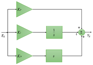
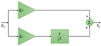
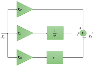
When the studies in the literature are examined, it is seen that in order to improve the control of AVR systems, either a new controller is proposed, a new optimisation algorithm is tried to optimally tune the parameters of the existing controllers, or a modified objective function is specified. 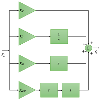First, it can be seen that proportional-integral-derivative (PID) [7,8,9], fractional order PID (FOPID) [9,10,11,12,13], and tilt-integral-derivative (TID) [14,15] controllers are widely used in the control of AVR systems. Fractional calculus-based FOPID and TID controllers can perform more successful control than PID controllers because they have more tuning parameters, and these tuning parameters have more flexible values. In addition to these, improved versions of PID and FOPID controllers, such as PID plus second-order derivative (PIDD²) [16,17,18], PID acceleration (PIDA) [7,19,20], sigmoid PID [21], sigmoid FOPID [22], FOPID with fractional filter (FOPIDFF) [23], FOPID plus fractional derivative (FOPIDD) [9,24], PID plus second-order derivative with filters (PIDND²N²) [25], cascaded real PID with second-order derivative and fractional order PI (RPIDD²-FOPI) [26], and tilt-fractional order integral-derivative with a second-order derivative and low-pass filters (TI^λDND²N²) [27] have been proposed to enhance the control efficiency of AVR systems.

Second, better tuning of the parameters of the controllers allows them to exhibit better control capability. Therefore, researchers prefer optimization algorithms via an objective function (OF) instead of traditional parameter tuning methods. These algorithms are either newly introduced algorithms or hybrid/enhanced versions of existing algorithms. In previous studies, it is seen that the whale optimization algorithm (WOA) [7], water cycle algorithm (WCA) [8], symbiotic organism search (SOS) [9], marine predator algorithm [11], seagull optimization algorithm [13], particle swarm optimization (PSO) [14,15,16], multiverse optimization algorithm (MVO) [17], bat algorithm (BA) [19], harmony search (HS) [20], dandelion optimizer (DO) [22], sin-cosine algorithm (SCA) [23], equilibrium optimizer (EO) [27], and gradient-based optimization (GBO) [28] are used in optimization processes under the control of the AVR system. In addition, improved/hybrid optimization algorithms such as the improved Jaya algorithm (IJA) [10], improved whale optimization algorithm (IWO) [18], and nonlinear sine cosine algorithm (NSCA) [21], are also used.

The better performance of the optimization algorithm is highly dependent on the OF used. When an OF suitable for the characteristic structure of the problem is used, the optimization process is more likely to be successful. The OFs frequently used in tuning the controller parameters of the AVR systems can be listed as Zwe-Lee Gaing (ZLG) [23,27], integral time absolute error (ITAE) [28,29], and integral time square error (ITSE) [30].

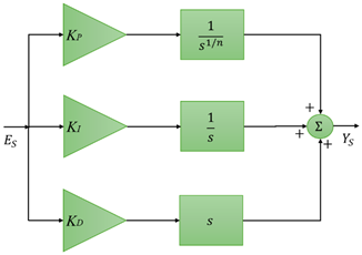
As can be seen from the abovementioned literature summary, efforts to enhance the control performance of AVR systems are mainly based on controller improvement. It is understood that the recently introduced controllers are mostly based on fractional order-based controllers. The extra tuning parameters provided by fractional calculus and its flexible control capability are the most important contributions to this trend. On the other hand, although many studies have been conducted on the development of FOPID controllers, studies on TID controllers are limited. It is known that feedback is of great importance in control systems. In addition, diversity in feedback has not been sufficiently studied in AVR systems. Therefore, it is worth investigating further consideration of feedback diversity and fractional calculus in the design of TID controllers. In this study, an I^λDND²N²-T controller is proposed to increase the control performance of AVR systems.

The major contributions of this study are summarized as follows:

✓

I^λDND²N²-T is proposed for the first time to maintain the terminal voltage of the AVR systems at the desired levels. The success of the controller in AVR systems reveals the potential for its use in solving many engineering problems.

✓

The performances of the EO, MVO, and PSO algorithms in solving the AVR problem are analysed, statistical tests are performed, and their successes are compared.

✓

The suitability of the EO algorithm, which gives better results than MVO and PSO, with the proposed controller and AVR systems is evaluated.

✓

The performance of the proposed I^λDND²N²-T controller is compared with PID-type controllers, such as PID, PIDD², PIDA, and FOPID, and hybrid controllers, including sliding mode control, fuzzy logic, and optimisation algorithms.

✓

The effectiveness of the proposed I^λDND²N²-T controller against disturbances such as generator frequency variation, load variation, and short circuit faults, which may occur in AVR systems, is validated experimentally.

✓

The robustness of the proposed controller on perturbed AVR system parameters is evaluated.

The remainder of this paper is organized as follows. Mathematical modelling of the AVR system is given in Section 2, a comprehensive definition of the proposed controller structure is provided in Section 3, used optimization algorithm and design of the objective function are presented in Section 4, results and discussion are reviewed in Section 5, and the conclusion is given in Section 6.

2. Mathematical Modelling of Automatic Voltage Regulator

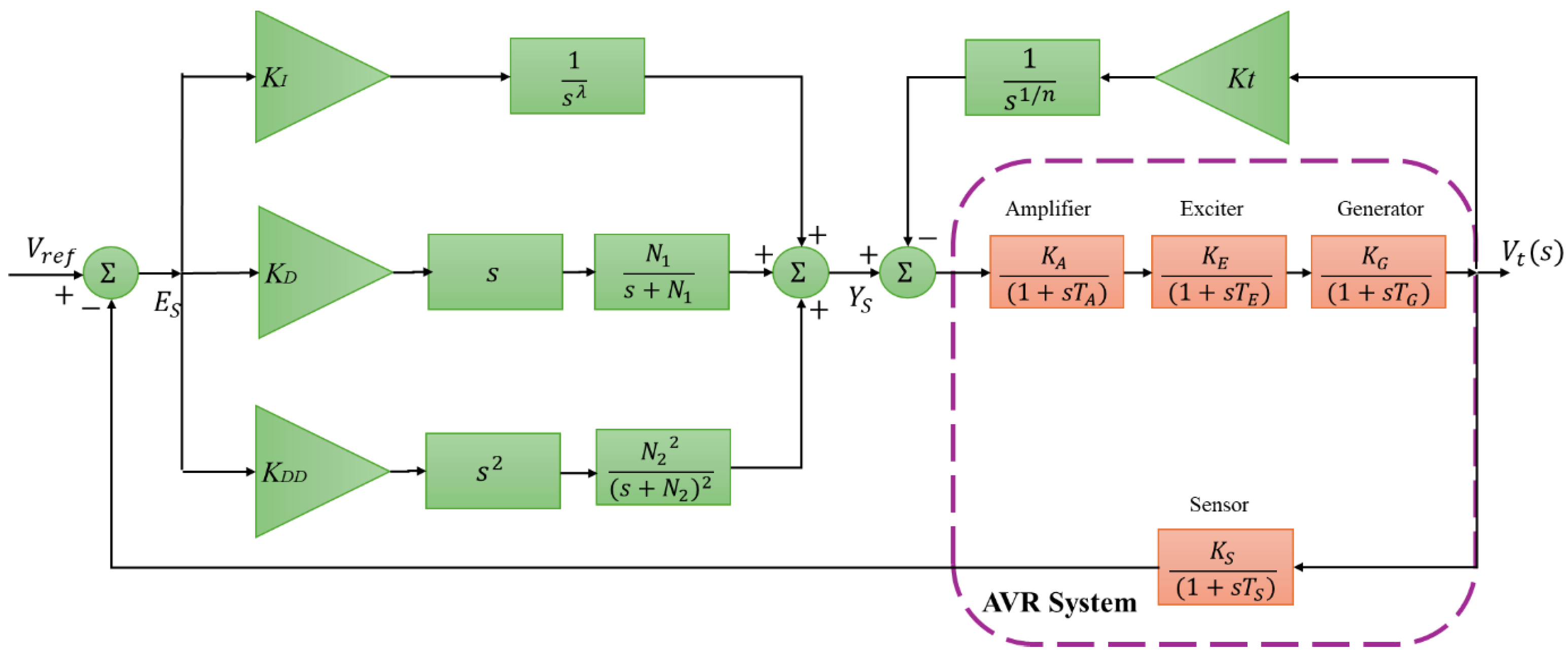
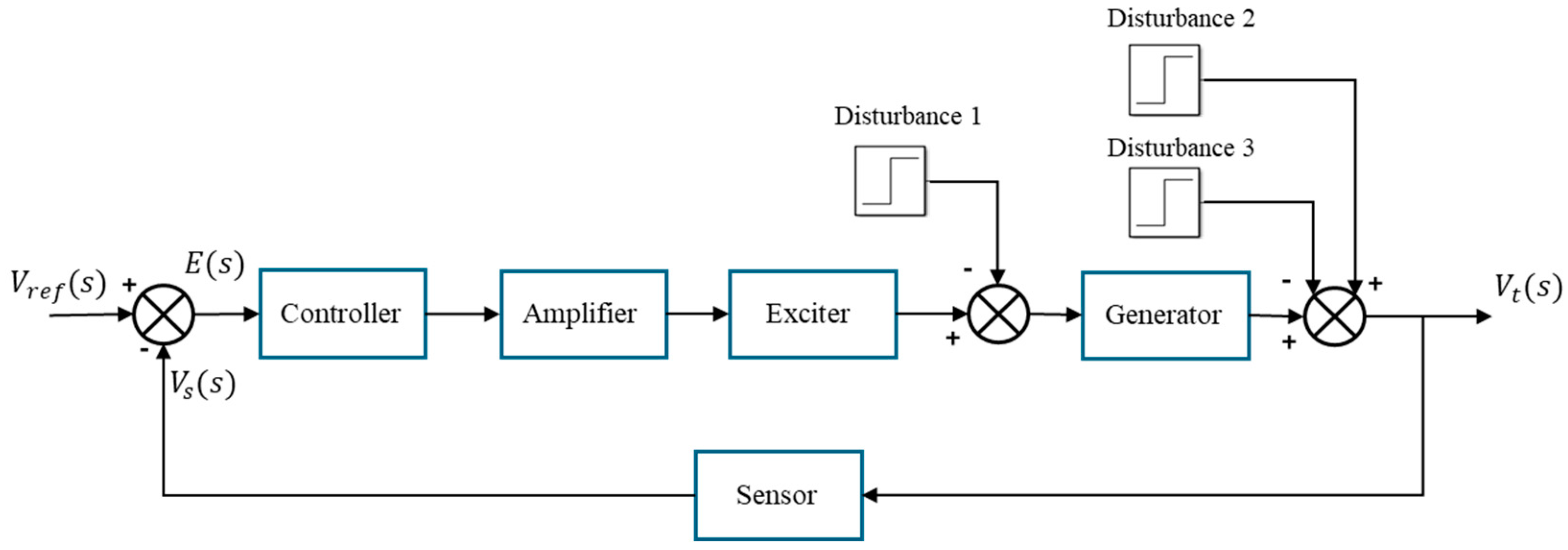
The AVR is responsible for keeping the terminal voltage constant and steady and plays an important role in the safety of power systems. The linearization of nonlinear systems is one of the widely preferred methods in engineering because of its ease of implementation and diversity of applications. In the studies, it is seen that control applications are performed on linearised AVR systems. The block diagram of the linearised AVR system consisting of amplifier, exciter, generator, and sensor is shown in Figure 1 [7,14,15,17,20]. In Figure 1, $V_{ref}$ is the reference voltage. E denotes the error signal, $V_s$ represents the output signal of sensor, and $V_t$ indicates the output voltage. The transfer functions of the system components and the ranges of the gain constants and time constants are summarized in

Table 1. Details of the components of the AVR system.

Components	Transfer Function	$\mathbf{Range} \mathbf{of} \mathbf{Gain} \mathbf{Value} \mathbf{\left(}\mathit{K}\mathbf{\right)}$	$\mathbf{Range} \mathbf{of} \mathbf{Time} \mathbf{Constant} \mathbf{\left(}{\mathit{T}}_{\mathit{S}}\mathbf{\right)}$
Amplifier	${\displaystyle \frac{K_A}{1+s{T}_A}}$	10–40	0.02–0.1
Exciter	${\displaystyle \frac{K_E}{1+s{T}_E}}$	1–10	0.4–1
Generator	${\displaystyle \frac{K_G}{1+s{T}_G}}$	0.7–1	1–2
Sensor	${\displaystyle \frac{K_S}{1+s{T}_S}}$	0.9–1.1	0.001–0.06

. In Table 1, $K_A$ and $T_A$ are the gain and time constants of the amplifier, $K_E$ and $T_E$ are the gain and time constants of the exciter, $K_G$ and $T_G$ are the gain and time constants of the generator, and $K_S$ and $T_S$ are the gain and time constants of the sensor.

The gain constants used for the amplifier, exciter, generator, and sensor are 10, 1, 1, and 1, respectively, and the time constants used for these components are 0.1, 0.4, 1, and 0.01. These values, selected from the gain and time constant ranges given in Table 1, are widely used in the literature [7,14,15,17,20]. Equation (1) gives the generalized closed-loop transfer function of the AVR system obtained using Figure 1.

$$G_{AVR}={\displaystyle \frac{G_A{G}_E{G}_G}{1+G_A{G}_E{G}_G{G}_S}}$$

(1)

Equation (2) gives the closed-loop transfer function of the AVR system derived from Table 1, Equation (1), and the values of the constants.

$${\mathrm{G}}_{\mathrm{A}\mathrm{V}\mathrm{R}}={\displaystyle \frac{0.1\mathrm{s}+10}{0.0004{\mathrm{s}}^4+0.0454{\mathrm{s}}^3+0.555{\mathrm{s}}^2+1.51\mathrm{s}+11}}$$

(2)

3. Design of Controller

3.1. Principle of Fractional Calculus

Although fractional calculus has a history of more than 300 years, fractional calculus-based controllers have been developed and implemented in recent years. Fractional order controllers (FOC) have better control capabilities than integer order controllers because they have more tuning parameters and behave more sensitively. The general description of FOC is given in Equation (3) [31].

$${}_a{}^{1}D_t^r=\left\{\begin{array}{c}{\displaystyle \frac{d^r}{{dt}^r}} R\left(r\right)>0,\\ 1 R\left(r\right)=0,\\ \underset{a}{\overset{t}{\int }}{\left(d\tau \right)}^{-r} R\left(r\right)<0\end{array}\right.$$

(3)

where $a$ and $t$ are the bounds of operation. $r\in R$ and $r$ is the fractional order of the integro-differential operator. The fractional derivative function can be stated with different mathematical expressions. The most preferred methods are Caputo, Grünwald–Letnikov (GL), and Riemann–Liouville (RL). rth order fractional derivative definition of Riemann–Liouville is given in Equation (4) [32,33].

$${}_a{}^{1}D_t^{r}f\left(t\right)={\displaystyle \frac{1}{\Gamma (n-r)}} {\displaystyle \frac{d^n}{{dt}^n}} {\int }_a^t{\displaystyle \frac{f\left(\tau \right)}{{(t-\tau )}^{r-n+1}}}d\tau , n-1<r<n$$

(4)

where $n$ is the integer section of $r$, $n\in N$. The Γ(.) depicts the Euler’s Gamma function.

An approximation is needed to implement the mathematical expressions given above in real-time applications of FOC, computer simulations, and discretization. Oustaloup’s recursive approximation (ORA) finds a solution for this. The ORA is used to implement the integro-differential operators in frequency domain and given in given Equation (5). The zeros, poles, and gain of the filter are described in Equations (6)–(8) [32].

$$s^r\approx K_f\prod _{k=-N}^N{\displaystyle \frac{s+w_k^{\prime }}{s+w_k}}$$

(5)

$$w_k=w_b{\left({\displaystyle \frac{w_h}{w_b}}\right)}^{{\displaystyle \frac{k+N+\frac{1}{2}(1+r)}{2N+1}}}$$

(6)

$$w_k^{\prime }=w_b{\left({\displaystyle \frac{w_h}{w_b}}\right)}^{{\displaystyle \frac{k+N+\frac{1}{2}(1-r)}{2N+1}}}$$

(7)

$$K_f=w_h^r$$

(8)

$r$ represents the differ-integration order, (2N + 1) is the analogue filter order, and $(w_b, w_h)$ is the range. The filter limits are chosen as [10⁻³ 10³] in this paper.

3.2. Integer Order Controller-Based AVR Systems

The most commonly utilized controllers in controlling AVR systems are integer-order PID-type controllers.

Table 2. The block diagrams and transfer function representations of integer order controllers.

Controller	Controller Block Diagram	Transfer Function Representation
PI		PI Controller
		$C_{PI}=K_P+{\displaystyle \frac{K_I}{s}}$
		AVR with PI Controller
		$G_{AVR PI}={\displaystyle \frac{C_{PI}{G}_A{G}_E{G}_G}{1+C_{PI}{G}_A{G}_E{G}_G{G}_S}}$
PID		PID Controller
		$C_{PID}=K_P+{\displaystyle \frac{K_I}{s}}+K_{D}s$
		AVR with PID Controller
		$G_{AVR PID}={\displaystyle \frac{C_{PID}{G}_A{G}_E{G}_G}{1+C_{PID}{G}_A{G}_E{G}_G{G}_S}}$
PIDD2		PIDD2 Controller
		$C_{PID{D}^2}=K_P+{\displaystyle \frac{K_I}{s}}+K_{D}s+{K_{DD}s}^2$
		AVR withPIDD2 Controller
		$G_{AVR PID{D}^2}={\displaystyle \frac{C_{PID{D}^2}{G}_A{G}_E{G}_G}{1+C_{PID{D}^2}{G}_A{G}_E{G}_G{G}_S}}$

presents the block diagrams and transfer function representations of the PI, PID, and PIDD² controllers frequently used in AVR.

$K_P$, $K_I$, $K_D,$ and $K_{DD}$ in the transfer function column of the Table 2 display the proportional, integral, derivative, and second-order derivative gains, respectively. Among these controllers, PI has two (K_P, K_I) PID has three (K_P, K_I, K_D) and PIDD² has four (K_P, K_I, K_D, K_DD) tuning parameters. The P, I, and D terms have different characteristics, and each of them has a different contribution to the control process. Therefore, as these parameters are added, the control functionality increases due to the increase in the number of tuning parameters and the contributions of the different characteristics.

In order to obtain a more stable output voltage in AVR systems, the PIDD² controller was derived by adding a second-order derivative part to the PID controller [16]. Thus, the acquired PIDD² controller can be successfully applied not only to AVR systems but also to other engineering problems.

3.3. Fractional Order Controller-Based AVR Systems

As explained in Section 3.1, the control capabilities of the systems are increased by improving integer-order PID-type controllers to fractional order-based controllers.

Table 3. The block diagrams and transfer function representations of fractional order controllers.

Controller	Controller Block Diagram	Transfer Function Representation
FOPI		FOPI Controller
		$C_{FOPI}=K_p+{\displaystyle \frac{K_i}{s^{\lambda }}}$
		AVR with FOPI Controller
		$G_{AVR FOPI}={\displaystyle \frac{C_{FOPI}{G}_A{G}_E{G}_G}{1+C_{FOPI}{G}_A{G}_E{G}_G{G}_S}}$
FOPID		FOPID Controller
		$C_{FOPID}=K_p+{\displaystyle \frac{K_i}{s^{\lambda }}}+K_d{s}^{\mu }$
		AVR with FOPID Controller
		$G_{AVR FOPID}={\displaystyle \frac{C_{FOPID}{G}_A{G}_E{G}_G}{1+C_{FOPID}{G}_A{G}_E{G}_G{G}_S}}$
TID		TID Controller
		$C_{TID}=K_t{\displaystyle \frac{1}{s^{\frac{1}{n}}}}+K_i{\displaystyle \frac{1}{S}}+K_{d}s$
		AVR with TID Controller
		$G_{AVR TID}={\displaystyle \frac{C_{TID}{G}_A{G}_E{G}_G}{1+C_{TID}{G}_A{G}_E{G}_G{G}_S}}$
FOTID		FOTID Controller
		$C_{FOTID}=K_t{\displaystyle \frac{1}{s^{\frac{1}{n}}}}+{\displaystyle \frac{K_i}{s^{\lambda }}}+K_d{s}^{\mu }$
		AVR with FOTID Controller
		$G_{AVR FOTID}={\displaystyle \frac{C_{FOTID}{G}_A{G}_E{G}_G}{1+C_{FOTID}{G}_A{G}_E{G}_G{G}_S}}$

presents the block diagrams and transfer function representations of Fractional Order PI (FOPI), Fractional Order PID (FOPID), Tilt-Integral-Derivative (TID), and Fractional order TID (FOTID) controllers.

The parameters $K_P$, $K_I$ and $K_D$ in Table 3 represent proportional, integral, and derivative gains, respectively. λ and µ are differential-integro parameters. Thus, extra tuning parameters are acquired compared to integer-order PI and PID controllers. While FOPI has 3 tuning parameters consisting of $K_P$, $K_I$, and λ, FOPID has 5 tuning parameters consisting of $K_P$, $K_I$, $K_D$, λ, and µ. In addition, because the PID controller is obtained when λ and µ are 1 in FOPID, it can be concluded that the FOPID controller also includes the PID controller.

The TID controller is obtained by multiplying the $K_P$ parameter of the integer-order-based PID controller by “ ${\displaystyle \frac{1}{s^{(1/n)}}}$”. The resulting part is called the “tilt” compensator and causes the TID controller to become a fractional order controller. Although the parameter n added to this controller varies according to the structure of the problem, it is usually taken between 1 and 10. It is taken as an optimisation parameter to determine the appropriate value for the target problem. This means that the TID controller has 4 tuning parameters consisting of $K_t$, $K_I$, $K_D,$ and n.

The FOTID controller is a hybrid version of the FOPID and TID controllers. All three gain parameters have become fractional order based due to the n, λ, and µ parameters. Thus, the FOTID controller has 6 tuning parameters consisting of $K_t$, $K_I$, $K_D$, n, λ, and µ.

3.4. Proposed Modified and Improved TID Controller

It is seen that well-controlled systems are desired by increasing the setting parameter and using the flexibility provided by fractional order. In this section, a new fractional order controller structure is proposed by modifying and improving the TID controller for the control of AVR systems. Figure 2 shows the block diagram of the proposed I^λDND²N²-T controller integrated with the AVR system. The I^λDND²N² controller is positioned before the system, and the input of the controller is the error (the difference between the reference and the sensor output) as in classical systems. The T controller leaves before the sensor and is connected to the previous controller with negative feedback. The desired and outstanding features with this controller are given below with their reasons.

• Since the proposed controller is a modified and improved version of the TID controller, it has the ease-of-use features of the TID controller and hence of the PID controller.
• Since the values of integro-differential parameters in fractional order controllers are in fractional degrees, they are capable of more sensitive tuning than integer order controllers.
• The PID controller has 3 tuning parameters, the TID controller has 4, the FOPID controller has 5, and the proposed controller has 8. Thus, controller intervention with different characteristics can be realized, and the system gains more precise control capability.
• The second-order derivative part in the proposed controller complies with the characteristic structure of AVR systems. Although this part improves the control of many engineering systems positively, improvements in the control of AVR come to the fore. The advantage of this part is used in the proposed controller.
• The filters used in both the first-order and second-order derivative term contribute to improved response, noise reduction, smoothing of the control action, and better stability.

Furthermore, the proposed controller includes integer order-based controllers. When n and λ values are 1, the “integral” ( ${\displaystyle \frac{K_i}{s^{\lambda }}}$) part and the “tilt” ( $K_t{\displaystyle \frac{1}{s^{\frac{1}{n}}}}$) part are converted to integer-order integral. As explained in Section 4, since the value of 1 is within the range of the lower and upper bound values of the coefficients of n and λ, this situation may occur after the optimization process.

4. Optimization Process and Objective Function

Equilibrium optimizer (EO) is a physics-based meta-heuristic algorithm and is proposed by Faramarzi [34]. EO attempts to achieve equilibrium states in the control volume. It imitates the dynamic and equilibrium cases associated with mass balance models where each concentration is randomly updated to reach the equilibrium case. The equation of mass balance is as follows:

$$V{\displaystyle \frac{dC}{dt}}=Q{C}_{eq}-QC+G$$

(9)

where V is the control volume (CV), C represents the CV concentration, and $V{\displaystyle \frac{dC}{dt}}$ is the variety rate of mass in CV. Q depicts the volumetric flow rate in coming and going out the CV. G is the rate of mass produced in the CV. $C_{eq}$ is the equilibrium state within the CV. Taking ${\displaystyle \frac{dC}{dt}}$ as a function of ${\displaystyle \frac{Q}{V}}$ and then applying some modifications, Equation (10) is obtained.

$$F=\exp \left[-\lambda \left(t-t_0\right)\right]$$

(10)

The λ given in Equation (10) is obtained during the adaptations and more details can be found in [34]. Where $t_0$ is the starting time based on the integration space.

• Initialization

Like other meta-heuristic optimization algorithms, EO requires an initial population to start the process. The initial concentrations are arranged according to the size and number of particles, and this is shown in Equation (11).

$$C_i^{initial}=C_{min}+{rand}_i\left(C_{max}+C_{min}\right) i=\mathrm{1,2},\dots n$$

(11)

$C_i^{initial}$ is the initial concentration. $C_{max}$ and $C_{min}$ are the maximum and minimum amounts. The vector ${rand}_i$ is a value that varies randomly between 0 and 1. $n$ depicts the population number.

• Equilibrium Pool and Candidates (Ceq)

In the EO algorithm, there are five candidate equilibrium particles, four of which are the best so far and one of which is the average of these four best particles. The vector formed by these five particles is shown in Equation (12).

$${\overrightarrow{C}}_{eq,pool}=\left\{ {\overrightarrow{C}}_{eq\left(1\right),}{ \overrightarrow{C}}_{eq\left(2\right), }{ \overrightarrow{C}}_{eq\left(3\right),} {\overrightarrow{C}}_{eq\left(4\right),} {\overrightarrow{C}}_{eq\left(ave\right) }\right\}$$

(12)

• Exponential Term

Equation (13), derived by modifications to Equation (10), is responsible for updating the concentration.

$$\overrightarrow{F}=a_{1}sign\left(\overrightarrow{k}-0.5\right)\left[e^{-\overrightarrow{\lambda }{\left(1-{\displaystyle \frac{Iter}{Ma{x}_{iter}}}\right)}^{\left(a_2{\displaystyle \frac{Iter}{Ma{x}_{iter}}}\right)}}-1\right]$$

(13)

$\overrightarrow{\mathsf{\lambda }}$ and $\overrightarrow{k}$ are vectors that vary randomly in the range 0–1. ${Max}_{iter}$ and $Iter$ indicate the maximum number of iterations and the current number of iteration, respectively. $a_1$ and $a_2$ are constant values related to the exploration and exploitation phases, respectively. In simulations, the effectiveness of the exploration and exploitation phases on the solution can be increased or decreased by increasing or decreasing the constant values $a_1$ and $a_2$. $sign(\overrightarrow{k}-0.5)$ determines the action of the exploitation and exploration.

• Generation Rate

The generation rate (G) improves the exploitation step to encounter better results. Expression of G is given in Equation (14).

$$\overrightarrow{G}=\left\{\begin{array}{c}0.5r_1\left({\overrightarrow{C}}_{eq}-\overrightarrow{\lambda }\overrightarrow{C}\right) \overrightarrow{F} ,k_2\ge GP\\ 0 , k_2<GP\end{array}\right.$$

(14)

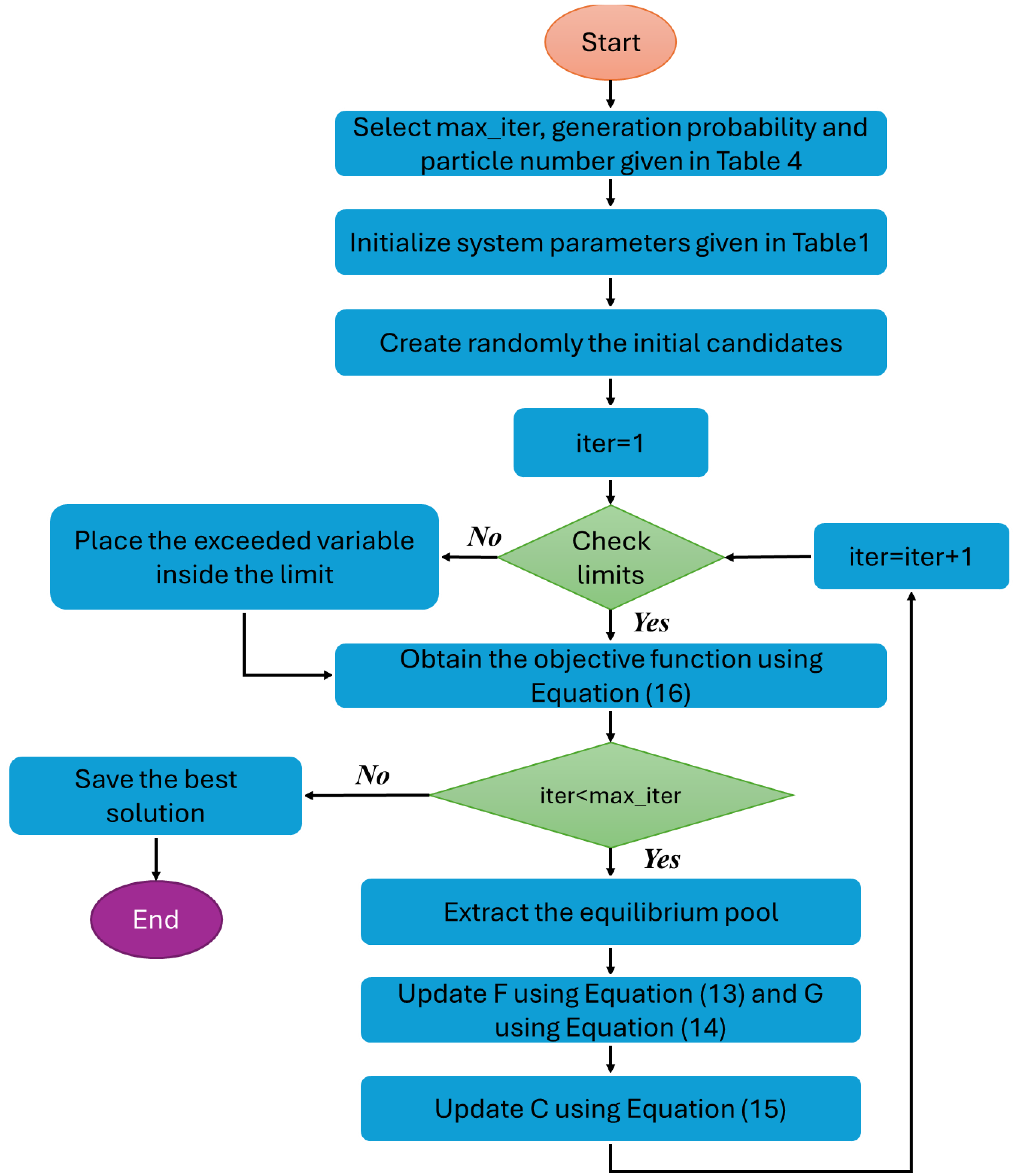
$k_1$ and $k_2$ are randomly varying numbers between 0 and 1. GP is the possibility of generation. This value was taken as 0.5 in this study in order to balance between the exploration and exploitation stages. Updating procedure of the EO is given in Equation (15).

$$C={\overrightarrow{C}}_{eq}+\left(\overrightarrow{C}-{\overrightarrow{C}}_{eq}\right)\overrightarrow{F}+{\displaystyle \frac{\overrightarrow{G}}{\overrightarrow{\lambda }V}}\left(1-\overrightarrow{F}\right)$$

(15)

The values taken for the experiments of the EO algorithm in this study are given in

Table 4. Experimental values of the EO algorithm.

Parameters	Values/Ranges
Iteration number	50
Population number	50
Variables number	8
$a_1$	2
$a_2$	1
GP	0.5
$k_1$$, k_2$	[0, 1]

. Figure 3 shows the flowchart of the EO algorithm.

An objective function is required for applying optimization methods to problems. Optimum controller parameters are obtained during the maximization or minimization of a selected objective function. In engineering problems, there are integral-based objective functions such as the integral absolute error (IAE), integral time absolute error (ITAE), integral square error (ISE), and integral time square error (ITSE), which are calculated directly from the error value (reference input-feedback), as well as objective functions obtained in accordance with the structure of the problem.

The objective function utilized in this study is widely used in AVR systems and provides successful results. The objective function is given in Equation (16) [35].

$$J=\left(1-e^{-\beta }\right).\left(M_p+E_{ss}\right)+e^{-\beta }.\left(t_s-t_r\right)$$

(16)

β is the weight coefficient, $M_p$ represents the overshoot, and $E_{ss}$ denotes steady-state error. $t_r$ and $t_s$ are rise time and settling time, respectively. β is generally taken between 0.5 and 1.5 in the literature. In the case of β > 0.7, steady-state error and overshoot drop and in the case of β < 0.7, the settling and rise time drop. It was taken as 0.5 in this study. Optimization parameters are $K_I$, $K_D$, $K_{DD}$, λ, $N_1$, $N_2$, $K_t,$ and n, for the I^λDND²N²-T controller. The lower and upper limits of these parameters are [0, 0, 0, 0.1, 10, 10, 0, 1], [5, 5, 5, 1.5, 500, 1000, 5, 10], respectively.

5. Results and Discussion

In this section, first, the parameters of the proposed controller are optimized using the EO, MVO, and PSO algorithms, and the most compatible optimization algorithm with the controller and AVR is determined. Then, the results of the proposed I^λDND²N²-T-EO are compared with the results presented in previous studies. In the following sections, the impact of possible disturbances on the AVR system outcome and the robustness test of the AVR system under perturbed system parameters are performed, respectively.

Matlab 2023a and Simulink were utilized in the realization of the experiments. The properties of the computer on which this study is conducted are intel i5-10400 CPU, 2.9 Ghz, 16 GB ram.

5.1. Achievement of the EO, MVO, and PSO Algorithms in AVR Systems with I^λDND²N²-T Controller

Firstly, the parameters of the proposed controller are optimized using the PSO, MVO, and EO algorithms. MVO stands out with its features, such as including parameters that increase the accuracy of local searches, emphasising local searches throughout the optimisation process, and increasing the convergence success by performing local searches proportionally to the number of iterations [36]. PSO is applied to many engineering problems with the advantages of having fewer tuning parameters and a high convergence speed [37,38]. In the EO algorithm, the random variation of the concentrations of the search agents allows the algorithm to avoid local optima throughout the optimisation process by improving the exploratory search in the initial iterations and the exploitative behaviour in the final iterations [34].

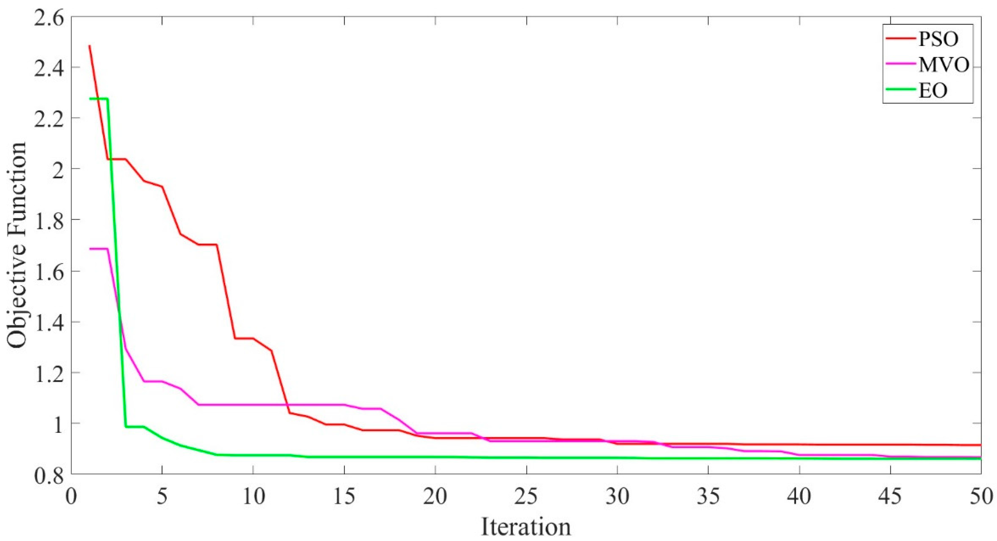
In this study, the experiments were repeated 30 times for each algorithm and the population and iteration numbers were taken as 50. Figure 4 shows the convergence curves of the utilized algorithms. Accordingly, while the MVO algorithm draws attention with its lower starting value, the EO algorithm falls to the lowest levels the fastest. The fact that the EO algorithm quickly converges to low objective function values shows that it will be successful at lower iteration numbers, but PSO and MVO cannot provide the same performance at low iteration numbers.

Table 5. Statistical tests of utilized optimization algorithms.

Algorithms	PSO	MVO	EO
Minimum	0.9154	0.8676	0.8621
Maximum	0.9985	0.9374	0.9092
Standart Deviation	0.0249	0.0240	0.0170
Mean	0.9534	0.9022	0.8764

presents the statistical tests of the PSO, MVO, and EO algorithms utilized in solving the AVR system problem. All optimization algorithms are run 30 times for each simulation study to contribute satisfying and powerful acceptance in the statistical analysis. Accordingly, it is seen that the EO algorithm exhibits better values in minimum, maximum, standard deviation, and mean values. Although MVO has a clear superiority over PSO in terms of minimum, maximum, and mean values, they are close to each other in terms of standard deviation. These results demonstrate that these two algorithms give similar results in terms of distances from the mean values.

Since the EO algorithm outperformed the PSO and MVO in this study, the controller parameters obtained with EO were used in the rest of this study.

5.2. Evaluation of I^λDND²N²-T Controller Performance

In this section, the achievement of the proposed I^λDND²N²-T EO controller is approved by comparing it with the PID-improved whale optimization algorithm (IWOA) [39], PID-multiverse optimizer (MVO) [17], PID-sin-cosine algorithm (SCA) [40], PID-artificial rabbits optimization algorithm (ARO) [41], PIDA-harmony search algorithm (HSA) [42], PIDA-teaching learned-based optimization (TLBO) [42], PIDA-WOA [7], PIDD²-PSO [16], PIDD²-EO [24], FOPID- marine predator optimization algorithm (MPA) [11], FOPID-heap-based optimization (HBO) [11], FOPID-hybridization of MPA and safe experimentation dynamics algorithm (MP-SEDA) [12], FOPID-seagull optimization algorithm (SOA) [13], FOPID-SCA [40], Fuzzy-PID [43], sliding mode control with grey wolf optimizer (SMC-GWO) [6], and sliding mode control with SCA (SMC-SCA) [6].

The methods chosen for comparison are derived from studies carried out in recent years.

Table 6. Parameters of related controllers.

Method	${\mathit{K}}_{\mathit{p}}/{\mathit{K}}_{\mathit{t}}$	${\mathit{K}}_{\mathit{i}}$	${\mathit{K}}_{\mathit{d}1}$	${\mathit{K}}_{\mathit{d}2}$	$\mathit{n}/{\mathit{K}}_{\mathit{a}}$	λ/α	μ/β	${\mathit{N}}_1$	${\mathit{N}}_2$
IλDND2N2-T EO	0.0012	4.9	1.6826	0.1424	7.3706	0.2958	-	33.3642	255.7196
FOPID MPA [11]	1.7061	0.8068	0.4000			1.1286	1.2164
FOPID HBO [11]	1.5215	0.7293	0.3601			1.1269	1.2073
FOPID MP SEDA [12]	2.9487	0.4533	0.4391			1.4016	1.4154
FOPID SOA [13]	0.9697	0.4918	0.2210			1.1522	1.1524
PID IWOA [39]	0.8167	0.6898	0.2799
PID MVO [17]	0.5971	0.4057	0.1980
PIDD2 EO [24]	3	2.0058	1.0936	0.0789
PIDD2 PSO [16]	2.7784	1.8521	0.9997	0.0739

presents the parameters of the related controllers.

Table 7. Transient response of the AVR system for various controllers.

	Controller–Algorithm	${\mathit{T}}_{\mathit{s}}$ (s)	${\mathit{T}}_{\mathit{r}}$ (s)	${\mathit{M}}_{\mathit{p}}$ (%)
Proposed	IλDND2N2-T	0.0564	0.0357	0.6724
PID	PID MVO [17]	0.5074	0.3264	0.0018
	PID IWOA [39]	0.6420	0.2120	9.56
	PID SCA [40]	0.3935	0.665	0.019
	PID WOA [7]	2.1359	0.2152	7.2570
	PID ARO [41]	0.9252	0.1747	1.1112
PIDA	PIDA WOA [7]	0.4996	0.3295	1.4087
	PIDA HSA [42]	1.0983	0.3073	0.4899
	PIDA TLBO [42]	1.1023	0.2758	0.6332
PIDD2	PIDD2 PSO [16]	0.1635	0.0929	0.0027
	PIDD2 EO [24]	0.1399	0.0829	0.0041
FOPID	FOPID MPA [11]	0.5886	0.1265	5.5051
	FOPID HBO [11]	0.6243	0.1429	3.4171
	FOPID MP SEDA [12]	0.3888	0.0793	3.5218
	FOPID SOA [13]	0.3975	0.2506	0
	FOPID SCA [40]	0.1660	0.2260	2.4223
Hybrid Controllers	Fuzzy PID [43]	0.6715	0.1225	20.6417
	Sliding mode control with GWO [6]	0.5431	0.3314	0.062
	Sliding mode control with SCA [6]	0.5444	0.3315	0

lists the time domain specifications, such as settling time, rise time, and overshoot of the terminal voltages of the AVR systems with different controllers. In Table 7, it can be seen that transient responses are high in AVR systems controlled by PID, whereas these values are lower in AVR systems controlled by FOPID. This is the main indicator of the increase in control performance from integer order to fractional order.

Also, it can be mentioned that the PIDA controllers perform slightly better than the PID controllers. This situation can be difficult to understand when the PID and PIDA controllers are directly compared in Table 7, but if the PID WOA and PIDA WOA controllers are compared, the superiority of PIDA over PID can be seen because the comparison conditions are equal. Considering the systems with PIDD² controller, it is seen that it exhibits better control ability than PID, FOPID, and PIDA due to the contribution of the second-order derivative term.

On the other hand, among the compared controllers, the proposed I^λDND²N²-T controller has the lowest settling time of 0.0564 s and the lowest rise time of 0.0357 s. In addition, it is one of the controllers with the lowest overshoot. The main reasons for this achievement are the extra second-order derivative term, the low-pass filters in both the first and second-order derivative parts, and the feedback tilt compensator.

Figure 5 shows the step response of the AVR system controlled by the proposed I^λDND²N²-T controller in this study and the proposed controllers in recently published papers. Since showing more studies in the same graph would make it difficult to understand the graph, only the studies whose controller parameters are given in Table 6 are shown in Figure 5. It is clear from Figure 5 that PID MVO decreases the overshoot of the terminal voltage and increases the settling time, whereas PID IWOA exhibits the opposite effect. It is also seen that FOPID controllers perform better than PID controllers, but they are not as successful as PIDD² controllers in terms of overshoot, settling time, and rise time values. On the other hand, it can be clearly observed that the proposed controller outperforms the compared controllers in terms of time domain specifications.

5.3. Controller Behaviour Against the Disturbance Effects

The controllers must maintain the stability of the system against disturbances in extraordinary situations. In simulation studies, disturbances are also taken as inputs in the systems. The difference between these disturbing inputs and the reference input of the system is that they are unpredictable regarding when and how large they are. Therefore, we investigated the impact of sufficiently large disturbances on the system and how the proposed controller copes with these disturbance effects.

Some effects that are likely to occur in AVR systems have been modelled as step functions and applied to the system. These effects are as follows:

• Disturbance 1: Disturbance 1 is considered as an input to model the deviation in the generator frequency and the effects of other generators in a multi-machine system. Disturbance 1 is applied at the 10th second with an amplitude of −1 pu and is performed before the generator as shown in Figure 6.
• Disturbance 2: Disturbance 2 is evaluated to model the load changes. Disturbance 2 is applied at the 20th second with an amplitude of +1 pu and is practiced after the generator as shown in Figure 6.
• Disturbance 3: Disturbance 3 is designed to model short circuit faults in the output voltage. Disturbance 3 is practiced at the 30th second with an amplitude of −1 pu and is applied after the generator as shown in Figure 6.

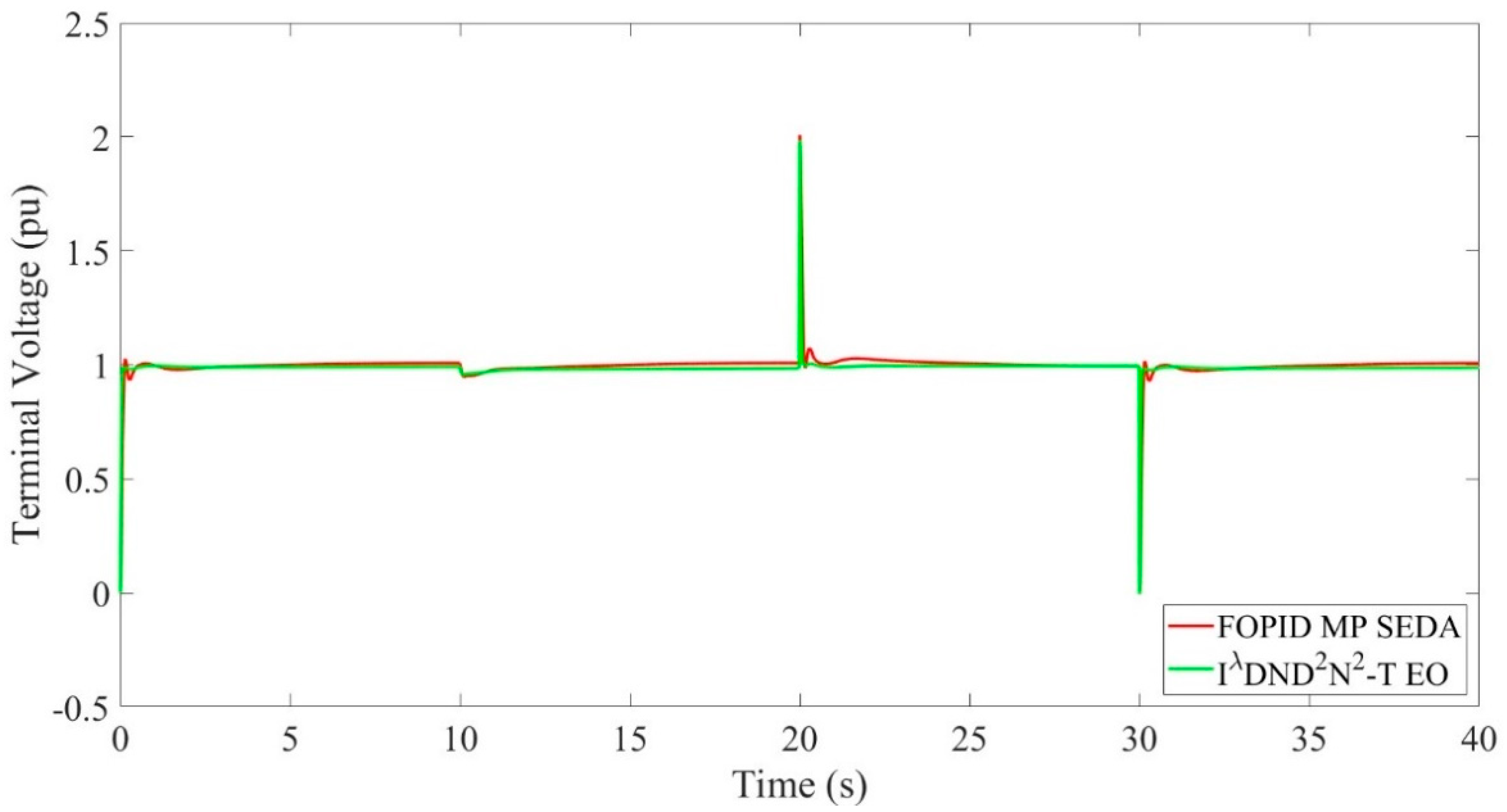
Figure 7 shows the step response of the AVR system’s terminal voltage against the modelled disturbances. In Figure 7, the AVR system is controlled by the proposed controller and FOPID MP SEDA, and the terminal voltage outputs are compared. According to the time domain characteristics in Table 7, the system controlled by FOPID MP SEDA was selected for comparison because it has the lowest rise time. It is clear from Figure 7 that after the Disturbance_1 is applied at t = 10 s, the proposed controller successfully restores the terminal voltage to the reference level. It reacts faster to disturbance than FOPID MP SEDA. The proposed controller has shown more favourable results than FOPID MP SEDA in terms of shortness of settling time and low fluctuation after the disturbance inputs applied at t = 20 s and t = 30 s. The proposed controller provides superior control against undesired and unexpected disturbance inputs.

5.4. Robustness Tests

Like all engineering systems, the AVR may not always work as desired, and due to external or internal effects, the time constants of its components may change. In order to examine the success of the proposed controller against such deteriorations in the system parameters, a robustness test is applied to the system. For this purpose, the time constants of the components are changed at the rates of $\pm$25% and $\pm$50%, and the time domain specifications obtained as a result of the changes are given in

Table 8. Transient response of the AVR system under perturbed system parameters.

Time Constants	Perturbation Variation (%)	Peak Value (pu)	${\mathit{T}}_{\mathit{s}}$ (s)	${\mathit{T}}_{\mathit{r}}$ (s)	${\mathit{T}}_{\mathit{p}}$ (s)
	Nominal Values	0.9999	0.0564	0.0357	0.9890
$T_A$	−50	1.1573	0.2930	0.0172	0.0390
	−25	1.0395	0.2049	0.0255	0.0510
	+25	1.0166	0.2017	0.0471	0.1560
	+50	1.0445	0.2660	0.0579	0.1630
$T_E$	−50	1.2835	0.3851	0.0160	0.0400
	−25	1.0866	0.1300	0.0243	0.0520
	+25	1.0002	0.1025	0.0520	0.1870
	+50	1.0093	0.2209	0.1870	0.2110
$T_G$	−50	1.3155	0.1834	0.0157	0.0410
	−25	1.0983	0.1209	0.0240	0.0530
	+25	1.0002	0.1173	0.0536	0.9390
	+50	1.0045	0.1431	0.0763	0.9170
$T_S$	−50	0.9960	0.1206	0.0478	1
	−25	0.9960	0.1123	0.0395	0.9940
	+25	1.0335	0.0911	0.0336	0.0700
	+50	1.0744	0.1067	0.0323	0.0710

and the step response is given in Figure 8.

According to Table 8, the highest value of the terminal voltage is 1.3155, where $T_G$ changes by −50%. The highest value of the settling time is 0.3851 s, where $T_E$ changes by −50% and the highest value of the rise time is 0.1870 s, where $T_E$ changes by +50%. As can be seen, the greatest effect on the rise and settling times is the change in $T_E$, while the change in the time constant $T_S$ in the sensor is not as effective as that of the other components.

The results indicate that even under the worst conditions, the AVR system with the proposed controller gives better results than an AVR system with PID and FOPID controllers operating under nominal conditions.

As can be seen in Figure 8, the distortions in $T_G$ lead to the highest peak value. After the deterioration caused by the changes in $T_G$, the highest deterioration is caused by the changes in $T_E$ and $T_A$, respectively. However, it should be clearly stated that there is not much difference between the nominal values of the AVR system components and the degraded system parameters.

6. Conclusions

In this paper, a fractional order integral-derivative plus second-order derivative with low-pass filters and tilt controller (I^λDND²N²-T) is proposed to keep the terminal voltage output at a constant value in AVR systems. In this study, EO, MVO, and PSO algorithms are used to optimise the controller parameters, among which the EO algorithm with the lowest objective function value and the best statistical test result is selected for this study. The superiority of the proposed controller in transient responses, such as settling time, rise time, and overshoot is demonstrated by comparing it with controllers proposed in previous studies. Afterwards, the achievement of the I^λDND²N²-T controller against disturbances such as generator frequency deviation, load variation, and short circuit current that may occur in AVR systems is expressed by simulations. Finally, the superior performance of the proposed controller against disturbances in the time constants of the amplifier, exciter, generator, and sensor in the AVR system is given in graphs and tables. As a result, the proposed controller can be successfully used to control AVR systems and can be used to control other engineering problems. In addition, the successful results of the proposed controller in this study may pave the way for testing it first on a prototype AVR system and then on a real-scale system. In future studies, the proposed controller will be applied to other problems in electrical and electronics engineering.