Seasonal Long Memory in Retail Sales in the G7 Countries

Abstract

This article examines the seasonal patterns of retail sales in the G7 nations, a key component of private consumption. Using seasonal fractional integration, we assess whether shocks present a lasting or temporary effect on retail sales trends, considering the high seasonal component. We observe mean reversion in France, Germany, Italy, Japan, and the UK, and permanent effects in the cases of Canada and USA. However, these outcomes vary based on the error term model applied. These results offer valuable information for policymakers seeking to boost consumption depending on the seasonal long memory property of the G7 countries.

1. Introduction

Private consumption accounts for 50 to 70% of GDP in advanced countries. Analyzing its trends and turning points helps consumers, investors, and policymakers understand a key part of business cycles and make more efficient decisions [1].

Private consumption may be tracked by using various economic indicators. One of them is household expenditure, monitored quarterly through National Accounts. Others are related to representative demand indicators such as retail sales, car registration, or electricity consumption, which are published monthly [2].

In this research paper, we focus on retail sales for two main reasons: first they represent a substantial portion of private consumption, spanning many sectors and including all types of companies [3]. Secondly, their time series presents strong seasonality, allowing researchers and analysts to identify patterns through seasonal fractional integration.

The historical series of many macroeconomic indicators, such as consumption, monetary aggregates, inflation, and income, are characterized by a strong persistent behavior in the form of a long memory, not only in the long-term but also at seasonal frequencies. However, the seasonal component is often overshadowed by the long-term trends in the data. Some authors, nevertheless, have investigated seasonal fractional integration techniques and their applications in relation to various financial and economic variables. Thus, for example, Gil-Alana [4] examined the GDP patterns in Denmark, Germany, and Italy using seasonal long memory techniques, enabling the simultaneous testing of multiple integration orders for each frequency. Gil-Alana [5] applied seasonal fractional integration techniques to investigate the US monthly money supply’s seasonal structure. He demonstrated that when seasonal monthly differences are employed instead of quarterly or first differences, the orders of integration are larger. He claims that when monthly seasonal roots are considered, the correlation between observations appears to be higher. In the same line of research, Gil-Alana et al. [6] employed seasonal fractional models to a Spanish tourism time series and identified seasonal long memory factors.

Cross-sectional aggregation, a common feature of many historical macroeconomic series, may produce seasonal frequencies with fractional orders of integration [7]. Candelon and Gil-Alana [8] proposed a method for evaluating unit roots and fractional integration at seasonal and long-term frequencies. They looked at four Latin American nations’ industrial production indices (Argentina, Brazil, Colombia, and Mexico). Their findings show long memory behavior in the seasonal structure of Brazil and Argentina, where shocks affect the seasonal form over time.

Arteche [9] also discussed methods for analyzing seasonal long memory and applied them to the Consumer Price Index from Spain. The main result indicates that data present a long memory for particular seasonal frequencies, but not all of them. Arteche [10] also conducted the same analysis after introducing the concept of volatility in the inflation series.

Gil-Alana et al. [11] examined persistence and seasonality in several retail sectors using seasonal and non-seasonal fractional integration models. Analyzing data from Australia and the US, the results indicate that the impacts of seasonality and persistence are not consistent across the various retail sectors. It is also evident that retail sales forecasts are better explained in terms of a long memory model that incorporates both persistence and seasonal components.

In another field, Yaya et al. [12] explored the seasonality and long-term dependence of observations and observed temporal trends in a climatological series using seasonal long memory techniques. They analyzed monthly precipitation data from 37 weather stations in six areas of Nigeria from 1981 to 2013. More recently, by taking into consideration the impacts of structural breaks and seasonality, Adekoya [13] used fractional integration methods to analyze the long memory behavior of American energy consumption. He found that energy consumption has a long memory, with persistence levels often varying between 0 and 1. The energy consumption series shows a noticeably strong seasonal pattern and autoregressive components, according to the estimated findings of the models with a seasonal impact and structural breakdowns.

An emerging research area involves the application of big data and machine learning to analyze private consumption patterns and retail sales. For example, recent studies have used data from payment systems (e.g., credit card transactions) to improve retail sales and consumption forecasts. These methods, employed by central banks and other policy institutions, offer valuable insights into real-time economic activity, as seen in research from the European Central Bank [14]. In the same line, Chapman and Desai [15] found that payment data with factor models can help improve accuracy by up to 25% in predicting GDP, retail, and wholesale sales in Canada, and nonlinear machine learning models can further improve the accuracy by up to 20%. These results are consistent with those of Bholat et al. [16] in the UK.

The literature reveals a gap in retail sales analysis. Most studies focus on individual countries and do not adequately account for seasonality. Furthermore, they do not apply seasonal fractional integration techniques for G7 countries, nor do they consider the impact of shocks on seasonal persistence.

In this regard, studying the seasonality of retail sales in G7 countries is particularly relevant, as the seasonal component is one of the most significant factors in consumption time series. Since G7 countries account for around 75% of the GDP of advanced economies, understanding retail sales patterns within a year is necessary for shaping effective fiscal and monetary policies. It is not only important to analyze the seasonality of retail sales, but also to assess the impact of shocks on the persistence of seasonality to accurately design demand-side policies.

The contributions of this research paper are twofold. First, our methodology (seasonal fractional integration) is accurate, enabling the study of macroeconomic indicators with a strong seasonal component such as a retail sales show (Ince and Taşdemir [17] clearly identify this pattern). In a situation with significant seasonality, this method will enable us to determine if shocks in the data are supposed to be temporary or long-lasting [11]. The paper emphasizes the extent to which demand policies should be restructured in response to permanent shocks affecting business cycles.

This is how the remainder of the article is configured. Section 2 describes the data that are exploited, Section 3 reviews the methodology applied, Section 4 reports the empirical outcomes, and Section 5 concludes and considers some of the policy consequences.

2. Data on Retail Sales in G7 Countries

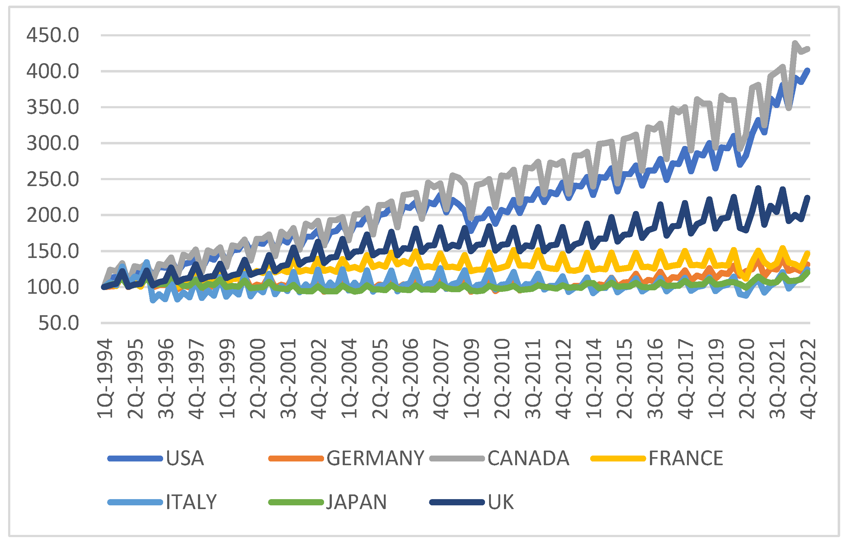
We used quarterly data on Total Retail Sales to measure private consumption across G7 countries from 1994 Q1 to 2022 Q4, allowing for analysis across various business cycles, including three big recession periods: Dotcom, Great Recession, and COVID. The data were collected from Thomson Reuters Eikon-Datastream, with original data sources from Canada (Statistics Canada), Japan (Ministry of Economy, Trade and Industry), the USA (U.S. Census Bureau), Germany (Federal Statistical Office), France (Banque de France), Italy (National Institute of Statistics), and the UK (Office for National Statistics). The time series were seasonally unadjusted and rebased to Q1-94 = 100 for homogeneous comparisons.

Using unadjusted quarterly data is essential when studying seasonal behavior year by year, as it enables the identification of peaks, such as those during Christmas, and troughs, like those in January.

Table 1. Descriptive analysis of retail sales.

	N	Minimum	Maximum	Mean	Stand. Dev.
USA	116	100.0	401.0	213.8	67.9
Germany	116	93.5	139.6	107.5	10.0
Canada	116	100.0	439.0	236.9	83.3
France	116	100.0	154.2	127.0	13.3
Italy	116	81.5	134.8	103.3	11.2
Japan	116	93.8	120.2	101.8	5.3
UK	116	100.0	237.5	157.5	33.0
N valid	116

displays the main descriptive statistics. The lowest level of retail sales was observed in Italy, while the highest value was found for Canada. Additionally, Canada, the US, and the UK have the highest means. Germany, Italy, and Japan have the lowest means. The three most volatile economies are those of Canada, the US, and the UK, where a bull trend can be appreciated. However, France, Italy, Germany and Japan reveal some evidence of stagnation (see Figure 1).

3. Seasonality

When analyzing seasonality in time series data, various approaches can be employed. One of them denotes deterministic seasonality and is based on the seasonal dummy variables. This approach is generally employed when the seasonal component is fixed across time. Stochastic approaches can be divided into stationary and non-stationary, and the classical distinction is between the seasonal Autoregressive Moving Average (ARMA) process for stationarity and the seasonal unit roots for non-stationarity. For the latter, several testing procedures are available for identifying unit roots, with the best-known being the Hylleberg, Engle, Granger, and Yoo [18] tests and their counterpart for monthly data, Beaulieu and Miron [19]. These two approaches can be combined into a more flexible model where the order of seasonal differentiation is a fractional value. This method is known as seasonal fractional integration and permits fractional degrees of differentiation with respect to the seasonal frequencies. Thus, it is more general and flexible than the classical models based on stationarity or unit roots and those that simply consider integer degrees of differentiation.

If a process can be represented in the following form, it is said to be seasonally fractionally integrated of order d and is designated as SFI(d) [4]:

(1 − L^s)^d x(t) = u(t), t = 1, 2

(1)

The amount of time periods per year is referred to as s.

The lag operator is L, i.e., Lx(t) = x(t − k), and u(t) is an I (0) process, which is a covariance stationary process whose spectral density function is positive and bounded at all frequencies. If d shows a positive sign in (1), x(t) follows a long memory process since the spectral density of the method displays singularities in the spectrum. For example, if s = 4, and d > 0, the spectrum of x(t) has poles at frequencies 0, π/2 and π/4 (3π/4) in the interval [0, π).

Seasonal long memory processes were first described by Jonas [20] and Abrahams and Dempster [21], while Carlin and Dempster [22] and Carlin et al. [23] extended this approach in a Bayesian framework. Using a parametric approach, Porter-Hudak [24] explored a model of seasonal fractional integration that is similar to the one given in Equation (1) regarding monetary supply from the USA and other purposes. The use of this modelization can be found in the work of Gil-Alana and Robinson [25], Ooms [26], and Silvapulle [27], while more recent contributions include those of Del Barrio Castro and Rachinger [28], Ben Nasr and Trabelsi [29], Koycegiz [30], and Yoshioka [31] among others.

Estimation was conducted using a general approach developed by Robinson [32] which is flexible enough to test any real value of arbitrary order anywhere on the unit circle in the complex plane. Thus, it allowed us to test for fractional seasonal differentiation. The specific test used for this particular case is detailed in the work of Gil-Alana and Robinson [25]. This method, based on the Lagrange Multiplier (LM) principle, relies on the likelihood function in the frequency domain. It has a standard limiting distribution, which holds independently of the inclusion of deterministic terms in the model like linear trends or seasonal dummies. Additionally, it is the most efficient method in the Pitman sense for detecting local departures [32]. Alternative approaches, such as the SARFIMA model in the work of Wilkins [33] or the semiparametric methods in the work of Arteche [34] or Reisen et al. [35] essentially lead to the same results as those reported in the following section.

4. Empirical Findings

The following model was examined:

Y(t) = γ₁S1(t) + γ₂S2(t) + γ₃S3(t) + γ₄S4(t) + γt + x(t), t = 1, 2, …

(2)

where x(t) follows an SFI(d) model as in Equation (1) and S1, S2, S3, and S4 refer to the seasonal dummy variables.

In

Table 2. SFI parameter estimations.

Series	White Noise	Seasonal AR(1)	Bloomfield
Canada	0.64 (0.36, 1.14)	1.36 (−0.91, 2.04)	0.09 (−1.64, 1.12)
France	0.55 (0.33, 1.11)	0.15 (−0.93, 1.67)	0.03 (−1.61, 1.08)
Germany	0.70 (0.35, 1.11)	0.15 (−0.89, 1.55)	0.08 (−1.63, 1.09)
Italy	0.60 (0.33, 1.14)	0.43 (−0.36, 1.97)	0.07 (−1.71, 1.11)
Japan	0.71 (0.34, 1.13)	0.19 (−0.24, 1.83)	0.05 (−1.64, 1.10)
UK	0.56 (0.34, 1.11)	0.33 (−1.76, 1.31)	−0.07 (−1.80, 1.08)
USA	0.76 (0.37, 1.16)	1.68 (1.24, 2.22)	0.10 (−1.76, 1.13)

, we display the results of d in Equations (1) and (2) considering three different specifications for the error term, i.e., u(t) in Equation (1). First, in column 2, u(t) is considered as a white noise method; in the following column, we suppose that it is a seasonal autoregressive, following an AR (1) process of form:

u(t) = ρ u(t−1) + ε(t), t = 1, 2, …

(3)

where ε(t) is a white noise process with constant variance and a mean equal to zero.

As observed in Table 2, when u(t) is white noise, the estimates are all smaller than 1, although the intervals are so wide that the unit root, i.e., d = 1, may not be rejected. If seasonal autoregressions are permitted, the values are very heterogenous; evidence of a d above 1 is obtained for Canada and the US while, for the rest of the countries, the values are below 1. In fact, every single nation, excluding the US, cannot reject the null of d = 0. Finally, we assume that the error term adheres to Bloomfield’s [36] exponential spectral model, which approximates the ARMA structures in the frequency domain. As we can observe, the I (0) hypothesis cannot be ruled out in any particular instance because all values of d are extremely close to zero. Depending on how the error term is modelled, the findings are notably varied. The seasonal dummy coefficients were discovered to be statistically irrelevant in all instances across all nations, despite not being stated; therefore, the hypothesis of deterministic seasonality for the series under examination was rejected.

From an economic standpoint, we can observe insights specific to each country. (1) In Canada, the relatively moderate randomness in retail sales indicates that Canadian policymakers could focus on smoothing out volatility through monetary policy adjustments. The presence of significant seasonality suggests that the government may want to encourage seasonal tax incentives or promote consumption during off-peak times. (2) France’s relatively weak seasonal trends and moderate white noise indicate more stable retail sales with fewer seasonal spikes. As a result, economic policies might focus more on long-term stability rather than short-term seasonal measures. (3) Germany, given its limited seasonality, could focus on broad economic reforms to promote continuous consumption, such as tax cuts or spending programs aimed at boosting retail demand in sectors that show weak seasonality. (4) Italy’s slightly higher seasonal component indicates that retail sales fluctuate with the seasons. Policymakers could take advantage of these periods by crafting seasonal incentives such as tourism or holiday-based promotions that can further boost sales during peak periods. (5) Japan’s data suggest minimal seasonal variation, which implies that retail sales are relatively stable year-round (like Germany). Policymakers might focus on ensuring long-term economic growth rather than addressing seasonal fluctuations. (6) The UK’s moderate randomness and low seasonal impact suggest that retail sales are more influenced by broader economic conditions rather than seasonal patterns. That means policymakers should focus on addressing economic uncertainties that may contribute to randomness in consumer behavior. Finally, (7) the U.S. has the most pronounced seasonal effect in retail sales, especially during periods like holidays and major shopping events (e.g., Black Friday). This strong seasonal pattern requires careful planning of monetary policy adjustments and stimulus efforts during key seasonal periods. Some policy actions could be oriented towards tax deductions or rebates timed around major retail seasons to maximize consumer spending. Additionally, the Federal Reserve could use these data to adjust interest rates and manage inflation more effectively during high-demand seasons.

5. Conclusions

This research investigated retail sails seasonality in G7 countries, an essential element of private consumption. We may highlight certain results and policy implications after using a seasonal fractional integration model to examine whether shocks in the series are predicted to be temporary or permanent in a context of high seasonality.

First, estimates for differencing parameter d for the retail sales in the G7 economies were all smaller than 1 if the disturbances were uncorrelated. However, since the intervals were very large, the unit root hypothesis (i.e., d = 1) may not be ruled out.

Second, the values of this parameter were very heterogeneous if seasonal autoregressions were allowed. As a result, evidence of d over 1 was obtained for Canada and the US, while these values were significantly lower for the other nations. This implies that in France, Germany, Italy, Japan, and the UK, shocks might be transitory but in Canada and the US we did not observe mean reversion, implying that the shocks were expected to have permanent effects. Therefore, policy actions should consider persistence in the analyzed countries. Policymakers can stimulate private consumption throughout the whole year in France, Germany, Japan, and the UK. Italy could take advantage of seasonal periods related to tourism. However, Americans should mainly focus on their weaker quarters.

Third, the error term was modeled with Bloomfield’s [36] exponential spectral model, which approximates ARMA structures in the frequency domain. Since all values of d were very near to 0, the I (0) or short memory hypothesis cannot be disproved in any particular instance. Thus, depending on how the error term is modelled, the findings are quite varied.

In conclusion, all this evidence provides insights and has implications for three main stakeholders. For Central Banks and policymakers, as retail sales are a key component of private consumption, the accurate forecasting of retail sales trends provides valuable insights into consumer behavior and economic health. Policymakers can better gauge economic momentum and implement timely interventions to stabilize or stimulate the economy as needed. Countries like France, Germany, Japan, and the UK might focus on long-term economic growth rather than seasonal fluctuations, and Italy (to lesser extent), Canada, and the US should design vigilant monetary and fiscal policy adjustments and stimulus during key seasonal periods. Retailers and businesses can leverage these advanced forecasting techniques to optimize inventory management, staffing, and marketing strategies based on more reliable sales predictions and trends. Finally, for researchers, the study demonstrates the potential of integration methods to assess the impact of shocks on sales, encouraging further exploration and methodological advancements in this area.