Understanding the Role of Intraspecific Disease Transmission and Quarantine on the Dynamics of Eco-Epidemiological Fractional Order Model

Abstract

An eco-epidemiological model involving competition regarding the predator and quarantine on infected prey is studied. The prey is divided into three compartments, namely susceptible, infected, and quarantine prey, while the predator only attacks the infected prey due to its weak condition caused by disease. To include the memory effect, the Caputo fractional derivative is employed. The model is validated by showing the existence, uniqueness, non-negativity, and boundedness of the solution. Three equilibrium points are obtained, namely predator-disease-free, predator-free-endemic, and predator-endemic points, which, respectively, represent the extinction of both predator and disease, the extinction of predator only, and the existence of all compartments. The local and global stability properties are investigated using the Matignon condition and the Lyapunov direct method. The numerical simulations using a predictor–corrector scheme are provided not only to confirm the analytical findings but also to explore more the dynamical behaviors, such as the impact of intraspecific competition, memory effect, and the occurrence of bifurcations.

1. Introduction

Different diseases may develop and spread among species when they interact in nature. The existence of these diseases plays an important role in controlling the dynamics of ecological systems. Through mathematical modeling, Anderson and May in 1986 [1] investigated disease factors in the predator–prey, host–parasite, and competitive systems and obtained the conclusion that the parasite’s basic reproduction number is a key factor in determining the structure and stability of the systems. Until now, the study of the intermingling of ecology and epidemiology, which is known as eco-epidemiology, has become an interesting research area in mathematical biology (see, for example, [2,3,4,5]).

In recent past years, the study of the dynamics of the predator–prey system under parasite infection has been completed by simplifying it into two cases, i.e., intraspecific and interspecific transmissions. Intraspecific transmission refers to the condition when the disease cannot cross over the species barrier. The disease only spreads either in the prey [6,7,8,9,10,11] or in the predator population [12,13,14,15,16]. Intraspecific transmission emerges from the interaction between two or more individuals of the same species that may occur in their socio-sexual system through grooming, mating, or fighting behaviors to obtain access to limited resources. These behaviors influence the transmission of parasites from individual to group and population levels [17]. In other cases, there is a condition when one species is susceptible to disease, and other species can also be infected. In this case, both prey and predator populations become multiple hosts for disease transmission [18,19,20]. After all, the main objective of this existing research is to examine how disease transmission affects conspecifics or other species when two or more species are associated. In addition, some of the research also studies the effect of the other factors of ecology in eco-epidemiology systems, such as prey refuge [21,22], harvesting [23,24], treatment of infected species [25,26], and the Allee effect [27,28,29]. Moreover, disease transmission can be reduced by separating infected individuals from their healthy groups through quarantine procedures. Quarantine refers to the temporary separation of animals before they are brought into a group or territory to stop the spread of contagious diseases among healthy populations. Some epidemic models, such as in [30,31,32], show how quarantine might reduce the incidence rate of the disease in the environment. Therefore, it is important to research how quarantine affects predator–prey interactions with the presence of disease in the prey. As far as we know, there is no focus investigation on the eco-epidemic model that we have previously described.

In modeling real-life problems, fractional differential equations have received much attention from various areas of research in applied sciences and engineering; see, for instance, [33,34,35,36,37]. The fractional derivatives could improve the accuracy of the model through their properties to tackle the process of forgetting the history [38,39]. A fractional order system leads to a good memory system that can capture all of the past events with the freedom of reducing the order of derivatives toward zero. In contrast to the integer order system, the process of forgetting an event takes place throughout a species’ life cycle due to the scenario of a particular time state. Some studies in [40,41,42] have identified the advantages of fractional order derivatives in modeling biological phenomena.

Motivated by the above in view, the main aim of the paper is to provide qualitative information on a fractional order eco-epidemiological model where there are quarantine places for the infected prey as a prophylactic strategy for the spread of the disease among the prey population hunted by predators, which are not affected by the disease. Accordingly, the structure of the paper is provided as follows. In Section 2, the mathematical model is constructed by providing some relevant assumptions. In Section 3, the existence, uniqueness, non-negativity, and boundedness of the solution, as well as the local and global stability of equilibrium points, are studied. However, Section 4 presents the numerical results to explore the most influential parameter through global sensitivity analysis and to investigate the impact of disease transmission, quarantine rate, and order of derivative in the dynamical behavior of the model. Finally, Section 5 contains all the mathematical findings of this study.

2. Model Formulation

In this section, we develop a predator–prey model based on the SIQ-Epidemic model (Susceptible-Infected-Quarantine) on prey that is hunted by a population of predator for food. The following assumption is provided to construct the model.

• The population of prey is divided into three compartments, namely susceptible prey, infected prey, and quarantine prey, which, respectively, are denoted by S, I, and Q.
• The birth rate of susceptible prey is assumed contantly symbolized by $\Lambda$.
• The susceptible prey is infected by disease with the disease transmission provided by a bilinear term βSI.
• As a human effort in protecting the ecological system, the infected prey is captured and quarantined with the quarantine rate proportional to the density of infected prey denoted by the linear term ηI. If the quarantined prey recovers, they will be returned to their natural habitat so that there is a risk of being reinfected. We denote the recovery rate by ζQ.
• The natural death rate of prey is provided by μ, and, hence, we have a natural death rate for each compartment symbolized by μS, μI, and μQ.
• The death rates caused by disease for infected and quarantined prey are, respectively, denoted by κI and φQ.
• The predator denoted by P only hunts the weak prey, in this case, the infected prey, and, hence, the susceptible prey is not being chased by the predator. The quarantine prey is also free from predation because it is in a place with human protection. We denote the predation rate of infected prey by ξIP.
• The birth rate of the predator is converted from the predation process provided by $\sigma$IP and the death rate of the predator provided by δP.
• Since the predator can only attack the infected prey, there is limited food availability for the predator. As an impact, there exists intraspecific competition regarding the predator with the death rate $\omega$P².

According to those assumptions, we construct the food chain and compartmental diagram as in Figure 1.

Based on the provided assumptions and the diagram in Figure 1, we develop a deterministic model using first-order derivative as follows.

$$\begin{array}{cc}\hfill {\displaystyle \frac{dS}{dt}}=& \Lambda -\mu S-\beta SI+\zeta Q,\hfill \\ \hfill {\displaystyle \frac{dI}{dt}}=& \beta SI-(\eta +\kappa +\mu )I-\xi IP,\hfill \\ \hfill {\displaystyle \frac{dQ}{dt}}=& \eta I-(\phi +\zeta +\mu )Q,\hfill \\ \hfill {\displaystyle \frac{dP}{dt}}=& \sigma IP-\delta P-\omega P^2.\hfill \end{array}$$

(1)

Biologically relevant examples for this model are found in [43], where pinniped tuberculosis affecting Malayan tapir (Tapirus indicus) with the predator is provided by jaguars and pumas; also, chronic wasting disease and bovine tuberculosis in wild and captive ungulates [44] with their obvious predators come from the carnivores. Health screening procedures while in quarantine for those animals are then provided in [45]. Now, consider the following definition.

Definition 1.

The Caputo fractional order derivative with the order-α is defined by [46]

$${}^C{\mathcal{D}}_t^{\alpha }w\left(t\right)=\frac{1}{\Gamma (1-\alpha )}{\int }_0^t{(t-s)}^{-\alpha }{w}^{\prime }\left(\tau \right)d\tau ,$$

(2)

where $\alpha \in (0,1]$, $t\ge 0,$$f\in C^n([0,+\infty ),\mathbb{R})$, and Γ is the Gamma function.

To include the memory effect, we then replace the operator of model (1) with the Caputo fractional order derivative provided by Definition 1. As a result, we have the fractional order model as follows.

$$\begin{array}{cc}\hfill {}^C{\mathcal{D}}_t^{\alpha }S=& \Lambda -\mu S-\beta SI+\zeta Q=F_1,\hfill \\ \hfill {}^C{\mathcal{D}}_t^{\alpha }I=& \beta SI-(\eta +\kappa +\mu )I-\xi IP=F_2,\hfill \\ \hfill {}^C{\mathcal{D}}_t^{\alpha }Q=& \eta I-(\phi +\zeta +\mu )Q=F_3,\hfill \\ \hfill {}^C{\mathcal{D}}_t^{\alpha }P=& \sigma IP-\delta P-\omega P^2=F_4.\hfill \end{array}$$

(3)

In the next section, we study the dynamical behaviors of model (3) by providing its analytical and numerical results as well as their biological interpretations.

3. Analytical Results

To facilitate the analytical process, we define the following feasible biological region.

$${\mathbb{R}}_{+}^4:=\{(S,I,Q,P)\in {\mathbb{R}}^4|S\ge 0,I\ge 0,Q\ge 0,P\ge 0\}.$$

Since the model describes the population dynamics, we have to ensure that the model (3) always has a solution for each provided non-negative initial condition. Moreover, the solution has to be unique since it is biologically impossible that two different conditions will arise in the future with the current single state. Thus, we provide the existence and uniqueness of the solution in Section 3.1. We also have to ensure that the solution is always non-negative and bounded in ${\mathbb{R}}_{+}^4$, which confirms the biological validity of the model. We provide these conditions in Section 3.2. Furthermore, the dynamics of model (3), including the feasible equilibrium points and their local and global stability, will be investigated.

3.1. Existence and Uniqueness of Solutions

We define the region

$$\mathcal{M}:=\left\{(S,I,Q,P)\in {\mathbb{R}}^4|max\left(\left|S\right|,\left|I\right|,\left|Q\right|,\left|P\right|\right)\le M\right\}.$$

Now, denote $X=\left(S,I,Q,P\right)$ and $\overline{X}=\left(\overline{S},\overline{I},\overline{Q},\overline{P}\right)$. Thus, for the mapping $F\left(X\right)=\left(F_1\left(X\right),F_2\left(X\right),F_3\left(X\right),F_4\left(X\right)\right)$ and for $X,\overline{X}\in \mathcal{M}$, we have

$$\begin{array}{cc}\hfill \left|F_1\left(X\right)-F_1\left(\overline{X}\right)\right|=& \left|\left(\Lambda -\mu S-\beta SI+\zeta Q\right)-\left(\Lambda -\mu \overline{S}-\beta \overline{S}\overline{I}+\zeta \overline{Q}\right)\right|\hfill \\ \hfill =& |-\mu \left(S-\overline{S}\right)-\beta I\left(S-\overline{S}\right)-\beta \overline{S}\left(I-\overline{I}\right)+\zeta \left(Q-\overline{Q}\right)|\hfill \\ \hfill \le & \mu |S-\overline{S}|+\beta M|S-\overline{S}|+\beta M|I-\overline{I}|+\zeta \left|Q-\overline{Q}\right|\hfill \\ \hfill =& \left(\mu +\beta M\right)|S-\overline{S}|+\beta M|I-\overline{I}|+\zeta |Q-\overline{Q}|,\hfill \\ \hfill \left|F_2\left(X\right)-F_2\left(\overline{X}\right)\right|=& |\left(\beta SI-(\eta +\kappa +\mu )I-\xi IP\right)-\left(\beta \overline{S}\overline{I}-(\eta +\kappa +\mu )\overline{I}-\xi \overline{I}\overline{P}\right)|\hfill \\ \hfill =& |\beta I\left(S-\overline{S}\right)+\beta \overline{S}\left(I-\overline{I}\right)-(\eta +\kappa +\mu )\left(I-\overline{I}\right)-\xi P\left(I-\overline{I}\right)-\xi \overline{I}\left(P-\overline{P}\right)|\hfill \\ \hfill \le & \beta M|S-\overline{S}|+\beta M|I-\overline{I}|+(\eta +\kappa +\mu )|I-\overline{I}|+\xi M|I-\overline{I}|+\xi M\left|P-\overline{P}\right|\hfill \\ \hfill =& \beta M|S-\overline{S}|+\left(\eta +\kappa +\mu +\left(\beta +\xi \right)M\right)|I-\overline{I}|+\xi M|P-\overline{P}|,\hfill \\ \hfill \left|F_3\left(X\right)-F_3\left(\overline{X}\right)\right|=& |\left(\eta I-(\phi +\zeta +\mu )Q\right)-\left(\eta \overline{I}-(\phi +\zeta +\mu )\overline{Q}\right)|\hfill \\ \hfill =& |\eta \left(I-\overline{I}\right)-(\phi +\zeta +\mu )\left(Q-\overline{Q}\right)|\hfill \\ \hfill \le & \eta |I-\overline{I}|+(\phi +\zeta +\mu )\left|Q-\overline{Q}\right|,\hfill \\ \hfill \left|F_4\left(X\right)-F_4\left(\overline{X}\right)\right|=& |\left(\sigma IP-\delta P-\omega P^2\right)-\left(\sigma \overline{I}\overline{P}-\delta \overline{P}-\omega {\overline{P}}^2\right)|\hfill \\ \hfill =& |\sigma P\left(I-\overline{I}\right)+\sigma \overline{I}\left(P-\overline{P}\right)-\delta \left(P-\overline{P}\right)-\omega \left(P+\overline{P}\right)\left(P-\overline{P}\right)|\hfill \\ \hfill \le & \sigma M|I-\overline{I}|+\sigma M|P-\overline{P}|+\delta |P-\overline{P}|+2\omega M\left|P-\overline{P}\right|\hfill \\ \hfill =& \sigma M|I-\overline{I}|+\left(\delta +\left(\sigma +2\omega \right)M\right)\left|P-\overline{P}\right|,\hfill \end{array}$$

and hence

$$\begin{array}{cc}\hfill ∥F\left(X\right)-F\left(\overline{X}\right)∥=& \left|F_1\left(X\right)-F_1\left(\overline{X}\right)\right|+\left|F_2\left(X\right)-F_2\left(\overline{X}\right)\right|+\left|F_3\left(X\right)-F_3\left(\overline{X}\right)\right|\hfill \\ \hfill & +\left|F_4\left(X\right)-F_4\left(\overline{X}\right)\right|\hfill \\ \hfill \le & \left(\mu +\beta M\right)\left|S-\overline{S}\right|+\beta M\left|I-\overline{I}\right|+\zeta \left|Q-\overline{Q}\right|\hfill \\ \hfill & +\beta M\left|S-\overline{S}\right|+\left(\eta +\kappa +\mu +\left(\beta +\xi \right)M\right)\left|I-\overline{I}\right|+\xi M\left|P-\overline{P}\right|\hfill \\ \hfill & +\eta \left|I-\overline{I}\right|+\left(\phi +\zeta +\mu \right)\left|Q-\overline{Q}\right|\hfill \\ \hfill & +\sigma M\left|I-\overline{I}\right|+\left(\delta +\left(\sigma +2\omega \right)M\right)\left|P-\overline{P}\right|\hfill \\ \hfill =& {\ell }_1\left|S-\overline{S}\right|+{\ell }_2\left|I-\overline{I}\right|+{\ell }_3\left|Q-\overline{Q}\right|+{\ell }_4\left|P-\overline{P}\right|\hfill \\ \hfill =& \ell ∥X-\overline{X}∥,\hfill \end{array}$$

where

$$\begin{array}{cccc}\hfill {\ell }_1=& \mu +2\beta M,\hfill & \hfill {\ell }_2=& 2\eta +\kappa +\mu +\left(2\beta +\xi +\sigma \right)M,\hfill \\ \hfill {\ell }_3=& \phi +2\zeta +\mu ,\hfill & \hfill {\ell }_4=& \delta +\left(\sigma +2\omega +\xi \right)M,\hfill \\ \hfill \ell =& max\left\{{\ell }_1,{\ell }_2,{\ell }_3,{\ell }_4\right\}.\hfill \end{array}$$

This confirms that F(X) satisfies the Lipschitz condition [47]. Obeying Theorem 3.4 in [48], if model (3) has initial value in ${\mathbb{R}}_{+}^4$, then the solution exists and is unique in the region $\mathcal{M}$. Therefore, the following theorem has been confirmed.

Theorem 1.

For any initial condition in${\mathbb{R}}_{+}^4$, the solution of model (3) always exists and is unique in the region $\mathcal{M}$.

3.2. Non-Negativity and Boundedness of Solutions

To show that $S\left(t\right)\ge 0$, $I\left(t\right)\ge 0$, $Q\left(t\right)\ge 0$, and $P\left(t\right)\ge 0$ as $t\to \infty$ for any initial condition in ${\mathbb{R}}_{+}^4$, we employ Theorem 6 provided by Cresson et al. [49]. Let $\alpha =1$ (first-order derivative given by model (1)). Thus, we can write the second and fourth equations in model (1) into the following equations.

$$\begin{array}{cc}\hfill {\displaystyle \frac{dI}{dt}}=& \left(\beta S-(\eta +\kappa +\mu )-\xi P\right)I,\hfill \\ \hfill {\displaystyle \frac{dP}{dt}}=& \left(\sigma I-\delta -\omega P\right)P.\hfill \end{array}$$

(4)

Hence, we obtain

$$\begin{array}{cc}\hfill I\left(t\right)=& I\left(0\right)e^{{\int }_0^t\left(\beta S\left(\tau \right)-(\eta +\kappa +\mu )-\xi P\left(\tau \right)\right)d\tau }\ge 0,\hfill \\ \hfill P\left(t\right)=& P\left(0\right)e^{{\int }_0^t\left(\sigma I\left(\tau \right)-\delta -\omega P\left(\tau \right)\right)d\tau }\ge 0.\hfill \end{array}$$

Since $I\left(t\right)\ge 0$, we can write the third equation in model (1) into the following equation.

$$\begin{array}{cc}\hfill {\displaystyle \frac{dQ}{dt}}=& \eta I-(\phi +\zeta +\mu )Q\hfill \\ \hfill \ge & -(\phi +\zeta +\mu )Q,\hfill \end{array}$$

Thus, we also have

$$Q\left(t\right)\ge Q\left(0\right)e^{-{\int }_0^t\left(\phi +\zeta +\mu \right)d\tau }\ge 0.$$

Next, from first equation in model (1) and the non-negativity of Q(t), we have

$$\begin{array}{cc}\hfill {\displaystyle \frac{dS}{dt}}=& \Lambda +\zeta Q-\left(\mu +\beta I\right)S\hfill \\ \hfill \ge & -\left(\mu +\beta I\right)S,\hfill \end{array}$$

which has solution

$$S\left(t\right)\ge S\left(0\right)e^{-{\int }_0^t\left(\mu +\beta I\right)d\tau }\ge 0.$$

Since S(t), I(t), Q(t), and P(t) are non-negative for $\alpha =1$ and the solution of model (3) satisfies the Lipschitz condition (see the proof of Theorem 1), Theorem 6 in [49] says that the model with Caputo fractional order provided by Equation (3) has non-negative solutions for all non-negative initial values. Therefore, we provide the following theorem as its results.

Theorem 2.

The solutions of model (3) with initial values in ${\mathbb{R}}_{+}^4$ are non-negative.

Now, we will show the boundedness of solutions of model (3). From Theorem 2, we construct a positive function as follows.

$$\mathcal{N}=S+I+Q+{\displaystyle \frac{\xi }{\sigma }}P.$$

(5)

The Caputo fractional order derivative of Equation (5) is

$${}^C{\mathcal{D}}_t^{\alpha }\mathcal{N}={}^C{\mathcal{D}}_t^{\alpha }S+{}^C{\mathcal{D}}_t^{\alpha }I+{}^C{\mathcal{D}}_t^{\alpha }Q+{\displaystyle \frac{\xi }{\sigma }}{}^C{\mathcal{D}}_t^{\alpha }P.$$

By continuing the calculation, we obtain the following inequality.

$$\begin{array}{cc}\hfill {}^C{\mathcal{D}}_t^{\alpha }\mathcal{N}=& {}^C{\mathcal{D}}_t^{\alpha }S+{}^C{\mathcal{D}}_t^{\alpha }I+{}^C{\mathcal{D}}_t^{\alpha }Q+{\displaystyle \frac{\xi }{\sigma }}{}^C{\mathcal{D}}_t^{\alpha }P\hfill \\ \hfill =& \left(\Lambda -\mu S-\beta SI+\zeta Q\right)+\left(\beta SI-(\eta +\kappa +\mu )I-\xi IP\right)\hfill \\ \hfill & +\left(\eta I-(\phi +\zeta +\mu )Q\right)+{\displaystyle \frac{\xi }{\sigma }}(\sigma IP-\delta P-\omega P^2)\hfill \\ \hfill =& \Lambda -\mu S-\mu I-\mu Q-{\displaystyle \frac{\mu \xi P}{\sigma }}-\kappa I-\phi Q-{\displaystyle \frac{\delta \xi P}{\sigma }}-{\displaystyle \frac{\xi \omega }{\sigma }}\left(P^2-{\displaystyle \frac{\mu }{\omega }}P\right)\hfill \\ \hfill =& \left(\Lambda +{\displaystyle \frac{{\mu }^2\xi }{4\sigma \omega }}\right)-\mu \mathcal{N}-\kappa I-\phi Q-{\displaystyle \frac{\delta \xi P}{\sigma }}-{\displaystyle \frac{\xi \omega }{\sigma }}{\left(P-{\displaystyle \frac{\mu }{2\omega }}\right)}^2\hfill \\ \hfill \le & \left(\Lambda +{\displaystyle \frac{{\mu }^2\xi }{4\sigma \omega }}\right)-\mu \mathcal{N}.\hfill \end{array}$$

Following Lemma 2.5 in [50], we obtain

$$\mathcal{N}\left(t\right)\le \left(\mathcal{N}\left(0\right)-\left({\displaystyle \frac{\Lambda }{\mu }}+{\displaystyle \frac{\mu \xi }{4\sigma \omega }}\right)\right)E_{\alpha }\left[-\mu t^{\alpha }\right]+\left({\displaystyle \frac{\Lambda }{\mu }}+{\displaystyle \frac{\mu \xi }{4\sigma \omega }}\right),$$

where E_α is the one-parameter Mittag–Leffler function. Following Lemma 5 in [51], we have $E_{\alpha }\left[-\mu t^{\alpha }\right]\to 0$ as $t\to \infty$. This means $\mathcal{N}\left(t\right)\to {\displaystyle \frac{\Lambda }{\mu }}+{\displaystyle \frac{\mu \xi }{4\sigma \omega }}$ as $t\to \infty$. Therefore, all solutions of model (3) enter to the region

$$\mathcal{K}:=\left\{(S,I,Q,P)\in {\mathbb{R}}^4|\mathcal{N}\le {\displaystyle \frac{\Lambda }{\mu }}+{\displaystyle \frac{\mu \xi }{4\sigma \omega }}+\epsilon ,\epsilon >0\right\}.$$

(6)

Finally, the following theorem holds.

Theorem 3.

The solutions of model (3) with initial values in ${\mathbb{R}}_{+}^4$ are uniformly bounded.

In the next subsections, we investigate the dynamical behaviors of model (3), such as the feasible equilibria, the basic reproduction number, local behaviors, and global dynamics. To identify the existence of equilibria, we solve $F_1=F_2=F_3=F_4=0$, which has four possible equations as follows.

$$\left\{\begin{array}{cc}\hfill \Lambda -\mu S-\beta SI+\zeta Q=& 0,\hfill \\ \hfill I=& 0,\hfill \\ \hfill \eta I-(\phi +\zeta +\mu )Q=& 0,\hfill \\ \hfill P=& 0.\hfill \end{array}\right.$$

(7)

$$\left\{\begin{array}{cc}\hfill \Lambda -\mu S-\beta SI+\zeta Q=& 0,\hfill \\ \hfill I=& 0,\hfill \\ \hfill \eta I-(\phi +\zeta +\mu )Q=& 0,\hfill \\ \hfill \sigma I-\delta -\omega P=& 0.\hfill \end{array}\right.$$

(8)

$$\left\{\begin{array}{cc}\hfill \Lambda -\mu S-\beta SI+\zeta Q=& 0,\hfill \\ \hfill \beta S-(\eta +\kappa +\mu )-\xi P=& 0,\hfill \\ \hfill \eta I-(\phi +\zeta +\mu )Q=& 0,\hfill \\ \hfill P=& 0.\hfill \end{array}\right.$$

(9)

$$\left\{\begin{array}{cc}\hfill \Lambda -\mu S-\beta SI+\zeta Q=& 0,\hfill \\ \hfill \beta S-(\eta +\kappa +\mu )-\xi P=& 0,\hfill \\ \hfill \eta I-(\phi +\zeta +\mu )Q=& 0,\hfill \\ \hfill \sigma I-\delta -\omega P=& 0.\hfill \end{array}\right.$$

(10)

The solution of Equations (7), (9), and (10) will be studied in Section 3.3, Section 3.4 and Section 3.5. Especially for Equation (8), when $I=0$, we have $P=-{\displaystyle \frac{\delta }{\omega }}<0$, and, hence, the solution not in ${\mathbb{R}}_{+}^4$, which states that the feasible equilibrium point does not exist for this condition. Moreover, to simplify the statement of the dynamical behavior, the locally and globally asymptotically stables are abbreviated by LAS and GAS. The LAS properties are obtained by applying linearization and obeying Matignon’s condition [52]. On the contrary, the GAS holds by constructing the Lyapunov function and investigating the sufficient condition; thus, the generalized LaSalle’s invariant principle provided by Huo et al. [53] is satisfied.

3.3. The Predator-Disease-Free Point and Basic Reproduction Number

The predator-disease-free point (PDFP) is obtained by solving Equation (7). We have PDFP as follows.

$${\mathcal{E}}_1=\left({\displaystyle \frac{\Lambda }{\mu }},0,0,0\right).$$

Furthermore, the basic reproduction number $\left({\mathcal{R}}_0\right)$ will be computed. The basic reproduction number $\left({\mathcal{R}}_0\right)$ is a parameter that is defined by the secondary infections caused by the primary infections in an uninfected population, which becomes the significant key in disease modeling since it can determine the spread of the disease in a population [54,55,56]. The next generation method is used to establish ${\mathcal{R}}_0$ [57]. Since the infectious compartments are I and Q, we can construct a Jacobian matrix of the new infection terms (F) and the remaining transfer terms (V) as follows.

$$F=\left[\begin{array}{cc}\beta S& 0\\ \eta & 0\end{array}\right]\mathrm{and}V=\left[\begin{array}{cc}(\eta +\kappa +\mu )+\xi P& 0\\ 0& \phi +\zeta +\mu \end{array}\right]$$

(11)

The basic reproduction number ${\mathcal{R}}_0$ is obtained by identifying the largest positive eigenvalue of FV⁻¹ [58,59]. We have

$$F{V}^{-1}=\left[\begin{array}{cc}{\displaystyle \frac{\beta S}{(\eta +\kappa +\mu )+\xi P}}& 0\\ {\displaystyle \frac{\eta }{(\eta +\kappa +\mu )+\xi P}}& 0\end{array}\right],$$

(12)

which provides eigenvalues ${\lambda }_1=0$ and ${\lambda }_2={\displaystyle \frac{\beta S}{(\eta +\kappa +\mu )+\xi P}}$, and, hence, by substituting ${\mathcal{E}}_1$, we have the following ${\mathcal{R}}_0$.

$${\mathcal{R}}_0={\displaystyle \frac{\beta \Lambda }{(\eta +\kappa +\mu )\mu }}.$$

(13)

Furthermore, the local and global dynamics around ${\mathcal{E}}_1$ are provided by the following theorem.

Theorem 4.

Let${\mathcal{R}}_0^a={\displaystyle \frac{\beta \Lambda }{\beta \Lambda +\mu \eta }}$. The PDFP ${\mathcal{E}}_1=\left({\displaystyle \frac{\Lambda }{\mu }},0,0,0\right)$ is a saddle point if ${\mathcal{R}}_0>1$, LAS if ${\mathcal{R}}_0<1$, and GAS if ${\mathcal{R}}_0<{\mathcal{R}}_0^a$.

Proof. 

We first identify the local dynamics of model (3) around ${\mathcal{E}}_1$. By linearization, the Jacobian matrix evaluated at ${\mathcal{E}}_1$ is

$${\mathcal{J}(S,I,Q,P)|}_{{\mathcal{E}}_1}=\left[\begin{array}{cccc}-\mu & -{\displaystyle \frac{\beta \Lambda }{\mu }}& \zeta & 0\\ 0& \left({\mathcal{R}}_0-1\right)(\eta +\kappa +\mu )& 0& 0\\ 0& \eta & -(\phi +\zeta +\mu )& 0\\ 0& 0& 0& -\delta \end{array}\right].$$

(14)

The eigenvalues of the Jacobian matrix (14) are ${\lambda }_1=-\mu$, ${\lambda }_2=\left({\mathcal{R}}_0-1\right)(\eta +\kappa +\mu )$, ${\lambda }_3=-(\phi +\zeta +\mu )$, and ${\lambda }_4=-\delta$. We confirm that $|arg\left({\lambda }_i\right)|=\pi >{\displaystyle \frac{\alpha \pi }{2}}$ for $i=$ 1, 3, 4. Therefore, the sign of ${\lambda }_2$ affects the local dynamics. When ${\mathcal{R}}_0<1$, we obtain $|arg\left({\lambda }_2\right)|=\pi >{\displaystyle \frac{\alpha \pi }{2}}$, and, hence, the Matignon condition [52] ensures that ${\mathcal{E}}_1$ is locally asymptotically stable. Moreover, when ${\mathcal{R}}_0>1$, it impacts $|arg\left({\lambda }_2\right)|=0<{\displaystyle \frac{\alpha \pi }{2}}$ and the PDFP becomes a saddle point.

Now, we study the sufficient condition so that GAS holds. To facilitate our work, the model (3) can be rewritten as

$$\begin{array}{cc}\hfill {}^C{\mathcal{D}}_t^{\alpha }S=& -\mu \left(S-{\displaystyle \frac{\Lambda }{\mu }}\right)-\beta SI+\zeta Q,\hfill \\ \hfill {}^C{\mathcal{D}}_t^{\alpha }I=& \beta SI-{\displaystyle \frac{\beta \Lambda I}{\mu {\mathcal{R}}_0}}-\xi IP,\hfill \\ \hfill {}^C{\mathcal{D}}_t^{\alpha }Q=& \eta I-(\phi +\zeta +\mu )Q,\hfill \\ \hfill {}^C{\mathcal{D}}_t^{\alpha }P=& \sigma IP-\delta P-\omega P^2.\hfill \end{array}$$

(15)

Next, we define a definite positive Volterra Linear Lyapunov function as follows.

$${\Phi }_1(S,I,Q,P)=\left(S-{\displaystyle \frac{\Lambda }{\mu }}-{\displaystyle \frac{\Lambda }{\mu }}ln{\displaystyle \frac{\mu S}{\Lambda }}\right)+I+Q+{\displaystyle \frac{\xi P}{\sigma }}.$$

(16)

Based on Lemma 3.1 in Vargas-De-León [60] along with system (15), the Caputo fractional order derivative of the Lyapunov function (16) is

$$\begin{array}{cc}\hfill {}^C{\mathcal{D}}_t^{\alpha }{\Phi }_1(S,I,Q,P)\le & \left({\displaystyle \frac{S-\Lambda /\mu }{S}}\right){}^C{\mathcal{D}}_t^{\alpha }S+{}^C{\mathcal{D}}_t^{\alpha }I+{}^C{\mathcal{D}}_t^{\alpha }Q+{\displaystyle \frac{\xi }{\sigma }}{}^C{\mathcal{D}}_t^{\alpha }P\hfill \\ \hfill =& \left({\displaystyle \frac{S-\Lambda /\mu }{S}}\right)\left(-\mu \left(S-{\displaystyle \frac{\Lambda }{\mu }}\right)-\beta SI+\zeta Q\right)+\left(\beta SI-{\displaystyle \frac{\beta \Lambda I}{\mu {\mathcal{R}}_0}}-\xi IP\right)\hfill \\ \hfill & +\left(\eta I-(\phi +\zeta +\mu )Q\right)+{\displaystyle \frac{\xi }{\sigma }}\left(\sigma IP-\delta P-\omega P^2\right)\hfill \\ \hfill =& -{\displaystyle \frac{\mu }{S}}{\left(S-{\displaystyle \frac{\Lambda }{\mu }}\right)}^2-\left({\displaystyle \frac{\beta \Lambda }{\beta \Lambda +\mu \eta }}-{\mathcal{R}}_0\right){\displaystyle \frac{\left(\beta \Lambda +\mu \eta \right)I}{\mu {\mathcal{R}}_0}}-(\phi +\mu )Q\hfill \\ \hfill & -{\displaystyle \frac{\delta \xi P}{\sigma }}-{\displaystyle \frac{\Lambda \zeta Q}{\mu S}}-{\displaystyle \frac{\xi \omega P^2}{\sigma }}\hfill \\ \hfill \le & -{\displaystyle \frac{\mu }{S}}{\left(S-{\displaystyle \frac{\Lambda }{\mu }}\right)}^2-\left({\displaystyle \frac{\beta \Lambda }{\beta \Lambda +\mu \eta }}-{\mathcal{R}}_0\right){\displaystyle \frac{\left(\beta \Lambda +\mu \eta \right)I}{\mu {\mathcal{R}}_0}}-(\phi +\mu )Q-{\displaystyle \frac{\delta \xi P}{\sigma }}\hfill \\ \hfill =& -{\displaystyle \frac{\mu }{S}}{\left(S-{\displaystyle \frac{\Lambda }{\mu }}\right)}^2-\left({\mathcal{R}}_0^a-{\mathcal{R}}_0\right){\displaystyle \frac{\left(\beta \Lambda +\mu \eta \right)I}{\mu {\mathcal{R}}_0}}-(\phi +\mu )Q-{\displaystyle \frac{\delta \xi P}{\sigma }}.\hfill \end{array}$$

As consequence, we have ${}^C{\mathcal{D}}_t^{\alpha }{\Phi }_1(S,I,Q,P)\le 0$ for all $(S,I,Q,P)\in {\mathbb{R}}_{+}^4$ when ${\mathcal{R}}_0<{\mathcal{R}}_0^a$. On the other hand, we confirm that ${}^C{\mathcal{D}}_t^{\alpha }{\Phi }_1(S,I,Q,P)=0$ only if $(S,I,Q,P)=\left({\displaystyle \frac{\Lambda }{\mu }},0,0,0\right)$. This emphasize that the singleton $\left\{{\mathcal{E}}_1\right\}$ is the only largest invariant set on which ${}^C{\mathcal{D}}_t^{\alpha }{\Phi }_1(S,I,Q,P)=0$. Thus, the generalized LaSalle’s invariant principle (Lemma 4.6 in [53]) guarantees that each solution in ${\mathbb{R}}_{+}^4$ tends to ${\mathcal{E}}_1$ for $t\to +\infty$. This ends the proof. □

Remark 1.

When conditions in Theorem 4 are satisfied, all populations will be extinct except the susceptible prey. More specifically, (i) if the LAS property is satisfied, this condition can happen when the initial condition is close enough to the value of the predator-disease-free point, and (ii) if the GAS property is satisfied, this condition can happen for all initial conditions.

3.4. The Predator-Free-Endemic Point

The predator-free-endemic point (PFEP) is acquired for the condition when the predator does not exist while each compartment of prey exists. The PFEP is obtained by solving Equation (9), which provides

$${\mathcal{E}}_2=\left(\widehat{S},\widehat{I},\widehat{Q},0\right),$$

where

$$\widehat{S}={\displaystyle \frac{\Lambda }{\mu {\mathcal{R}}_0}},\widehat{I}={\displaystyle \frac{\left(\phi +\zeta +\mu \right)\widehat{Q}}{\eta }},\mathrm{and}\widehat{Q}={\displaystyle \frac{\left({\mathcal{R}}_0-1\right)\eta \Lambda }{\left(\left(\phi +\mu \right)\eta +\left(\phi +\zeta +\mu \right)\left(\kappa +\mu \right)\right){\mathcal{R}}_0}}.$$

Remark 2.

We ensure that the PFEP exists only if ${\mathcal{R}}_0>1$. We also confirm from Theorem 4 that, when PFEP exists, the PDFP is a saddle point (unstable).

Theorem 5.

The PFEP ${\mathcal{E}}_2=\left(\widehat{S},\widehat{I},\widehat{Q},0\right)$ is LAS if ${\mathcal{R}}_0>1$, $\widehat{I}<{\displaystyle \frac{\delta }{\sigma }}$, and (i) ${\Delta }_a>0$ and $a_1{a}_2>a_3$, or (ii) ${\Delta }_a<0$ and $\alpha <2/3$ or $a_1{a}_2=a_3$, where

$$\begin{array}{cc}\hfill {\Delta }_a=& 18a_1{a}_2{a}_3+a_1^2{a}_2^2-4a_1^3{a}_3-4a_2^3-27a_3^2\hfill \\ \hfill a_1=& (\beta \widehat{I}+\mu )+(\phi +\zeta +\mu )\hfill \\ \hfill a_2=& {\displaystyle \frac{{\beta }^2\Lambda \widehat{I}}{\mu {\mathcal{R}}_0}}+\left(\beta \widehat{I}+\mu \right)\left(\phi +\zeta +\mu \right)\hfill \\ \hfill a_3=& \left(\left(\mu +\phi \right)\eta +\left(\kappa +\mu \right)\left(\phi +\zeta +\mu \right)\right)\beta \widehat{I}\hfill \end{array}$$

Proof. 

The Jacobian matrix for ${\mathcal{E}}_2$ is provided by

$${\mathcal{J}(S,I,Q,P)|}_{{\mathcal{E}}_2}=\left[\begin{array}{cccc}-\left(\beta \widehat{I}+\mu \right)& -{\displaystyle \frac{\beta \Lambda }{\mu {\mathcal{R}}_0}}& \zeta & 0\\ \beta \widehat{I}& 0& 0& -\xi \widehat{I}\\ 0& \eta & -(\phi +\zeta +\mu )& 0\\ 0& 0& 0& \sigma \widehat{I}-\delta \end{array}\right],$$

which provides an eigenvalue ${\lambda }_1=\sigma \widehat{I}-\delta$, and three other eigenvalues are solutions of the following polynomial characteristic.

$$P\left(\lambda \right)={\lambda }^3+a_1{\lambda }^2+a_2\lambda +a_3.$$

(17)

Since $\widehat{I}<{\displaystyle \frac{\delta }{\sigma }}$, we have $|arg\left({\lambda }_1\right)|=\pi >{\displaystyle \frac{\alpha \pi }{2}}$. For ${\lambda }_i,i=$ 2, 3, 4, by obeying the Routh–Hurwitz theorem for a model with Caputo fractional order derivative proposed by Ahmed et al. [61], we have ${\Delta }_a$, which is the discriminant of polynomial (17) and Proposition 1 on [61], which completes the rest of the proof. □

Next, the global stability of PFEP ${\mathcal{E}}_2=\left(\widehat{S},\widehat{I},\widehat{Q},0\right)$ will be determined. We first rewrite model (3) into the following system.

$$\begin{array}{cc}\hfill {}^C{\mathcal{D}}_t^{\alpha }S=& -\left(\mu +\beta I\right)\left(S-\widehat{S}\right)-\beta \widehat{S}\left(I-\widehat{I}\right)+\zeta \left(Q-\widehat{Q}\right),\hfill \\ \hfill {}^C{\mathcal{D}}_t^{\alpha }I=& \beta I\left(S-\widehat{S}\right)-\xi P\left(I-\widehat{I}\right)-\xi \widehat{I}P,\hfill \\ \hfill {}^C{\mathcal{D}}_t^{\alpha }Q=& \eta \left(I-\widehat{I}\right)-(\phi +\zeta +\mu )\left(Q-\widehat{Q}\right),\hfill \\ \hfill {}^C{\mathcal{D}}_t^{\alpha }P=& \sigma IP-\delta P-\omega P^2.\hfill \end{array}$$

(18)

Next, we construct a Quadratic Volterra Linear Lyapunov function as follows [60,62].

$${\Phi }_2(S,I,Q,P)={\displaystyle \frac{{\left(S-\widehat{S}\right)}^2}{2\widehat{S}}}+\left(I-\widehat{I}-\widehat{I}ln{\displaystyle \frac{I}{\widehat{I}}}\right)+{\displaystyle \frac{{\left(Q-\widehat{Q}\right)}^2}{2\widehat{Q}}}+{\displaystyle \frac{\xi P}{\sigma }}.$$

(19)

Applying Lemma 3.1 in [60], Lemma 2.3 in [62], and Equation (18), the Lyapunov function (16) has the Caputo fractional order derivative as follows.

$$\begin{array}{cc}\hfill {}^C{\mathcal{D}}_t^{\alpha }{\Phi }_2(S,I,Q,P)\le & \left({\displaystyle \frac{S-\widehat{S}}{\widehat{S}}}\right){}^C{\mathcal{D}}_t^{\alpha }S+\left({\displaystyle \frac{I-\widehat{I}}{I}}\right){}^C{\mathcal{D}}_t^{\alpha }I+\left({\displaystyle \frac{Q-\widehat{Q}}{\widehat{Q}}}\right){}^C{\mathcal{D}}_t^{\alpha }Q+{\displaystyle \frac{\xi }{\sigma }}{}^C{\mathcal{D}}_t^{\alpha }P\hfill \\ \hfill =& \left({\displaystyle \frac{S-\widehat{S}}{\widehat{S}}}\right)\left(-\left(\mu +\beta I\right)\left(S-\widehat{S}\right)-\beta \widehat{S}\left(I-\widehat{I}\right)+\zeta \left(Q-\widehat{Q}\right)\right)\hfill \\ \hfill & +\left({\displaystyle \frac{I-\widehat{I}}{I}}\right)\left(\beta I\left(S-\widehat{S}\right)-\xi P\left(I-\widehat{I}\right)-\xi \widehat{I}P\right)\hfill \\ \hfill & +\left({\displaystyle \frac{Q-\widehat{Q}}{\widehat{Q}}}\right)\left(\eta \left(I-\widehat{I}\right)-(\phi +\zeta +\mu )\left(Q-\widehat{Q}\right)\right)\hfill \\ \hfill & +{\displaystyle \frac{\xi }{\sigma }}\left(\sigma IP-\delta P-\omega P^2\right)\hfill \\ \hfill =& -{\displaystyle \frac{\left(\mu +\beta I\right)}{\widehat{S}}}{\left(S-\widehat{S}\right)}^2+{\displaystyle \frac{\zeta }{\widehat{S}}}\left(S-\widehat{S}\right)\left(Q-\widehat{Q}\right)\hfill \\ \hfill & -\left({\displaystyle \frac{\delta }{\sigma }}-\widehat{I}\right)\xi P-{\displaystyle \frac{\eta \widehat{I}Q}{\widehat{Q}}}+{\displaystyle \frac{\eta IQ}{\widehat{Q}}}-\eta I+\eta \widehat{I}\hfill \\ \hfill & -{\displaystyle \frac{(\phi +\zeta +\mu )}{\widehat{Q}}}{\left(Q-\widehat{Q}\right)}^2-{\displaystyle \frac{\xi \omega P^2}{\sigma }}\hfill \\ \hfill \le & -{\displaystyle \frac{\mu }{\widehat{S}}}{\left(S-\widehat{S}\right)}^2+{\displaystyle \frac{\zeta }{2\widehat{S}}}{\left(S-\widehat{S}\right)}^2+{\displaystyle \frac{\zeta }{2\widehat{S}}}{\left(Q-\widehat{Q}\right)}^2\hfill \\ \hfill & -\left({\displaystyle \frac{\delta }{\sigma }}-\widehat{I}\right)\xi P-\left(1-{\displaystyle \frac{I}{\widehat{I}}}\right)\left({\displaystyle \frac{Q}{\widehat{Q}}}-1\right)\eta \widehat{I}\hfill \\ \hfill & -{\displaystyle \frac{(\phi +\zeta +\mu )}{\widehat{Q}}}{\left(Q-\widehat{Q}\right)}^2\hfill \end{array}$$

Thus, in the region,

$${\widehat{\Psi }}_1:=\left\{(S,I,Q,P)|min\left\{{\displaystyle \frac{\widehat{I}}{I}},{\displaystyle \frac{Q}{\widehat{Q}}}\right\}>1,\mathrm{or}max\left\{{\displaystyle \frac{\widehat{I}}{I}},{\displaystyle \frac{Q}{\widehat{Q}}}\right\}<1\right\},$$

we have

$$\begin{array}{cc}\hfill {}^C{\mathcal{D}}_t^{\alpha }{\Phi }_2(S,I,Q,P)\le & -{\displaystyle \frac{\mu }{\widehat{S}}}{\left(S-\widehat{S}\right)}^2+{\displaystyle \frac{\zeta }{2\widehat{S}}}{\left(S-\widehat{S}\right)}^2+{\displaystyle \frac{\zeta }{2\widehat{S}}}{\left(Q-\widehat{Q}\right)}^2\hfill \\ \hfill & -\left({\displaystyle \frac{\delta }{\sigma }}-\widehat{I}\right)\xi P-{\displaystyle \frac{(\phi +\zeta +\mu )}{\widehat{Q}}}{\left(Q-\widehat{Q}\right)}^2\hfill \\ \hfill =& -\left(\mu -{\displaystyle \frac{\zeta }{2}}\right){\displaystyle \frac{{\left(S-\widehat{S}\right)}^2}{\widehat{S}}}-\left({\displaystyle \frac{(\phi +\zeta +\mu )}{\widehat{Q}}}-{\displaystyle \frac{\zeta }{2\widehat{S}}}\right){\left(Q-\widehat{Q}\right)}^2\hfill \\ \hfill & -\left({\displaystyle \frac{\delta }{\sigma }}-\widehat{I}\right)\xi P.\hfill \end{array}$$

Substituting the value of $\widehat{S}$, we acquire

$$\begin{array}{cc}\hfill {}^C{\mathcal{D}}_t^{\alpha }{\Phi }_2(S,I,Q,P)\le & -\left(\mu -{\displaystyle \frac{\zeta }{2}}\right){\displaystyle \frac{{\left(S-\widehat{S}\right)}^2}{\widehat{S}}}-\left({\displaystyle \frac{(\phi +\zeta +\mu )}{\widehat{Q}}}-{\displaystyle \frac{\mu \zeta {\mathcal{R}}_0}{2\Lambda }}\right){\left(Q-\widehat{Q}\right)}^2\hfill \\ \hfill & -\left({\displaystyle \frac{\delta }{\sigma }}-\widehat{I}\right)\xi P\hfill \end{array}$$

Therefore, ${}^C{\mathcal{D}}_t^{\alpha }{\Phi }_2(S,I,Q,P)\le 0$ if $\zeta <2\mu$, ${\mathcal{R}}_0<{\displaystyle \frac{2(\phi +\zeta +\mu )\Lambda }{\mu \zeta \widehat{Q}}}$, and $\widehat{I}<{\displaystyle \frac{\delta }{\sigma }}$. Obeying Lemma 4.6 in [53] along with the existence condition of PFEP, the following theorem is provided as a result.

Theorem 6.

The PFEP ${\mathcal{E}}_2=\left(\widehat{S},\widehat{I},\widehat{Q},0\right)$ is GAS in the region ${\widehat{\Psi }}_1$ if $1<{\mathcal{R}}_0<{\mathcal{R}}_0^b$, $\zeta <2\mu$, and $\widehat{I}<{\displaystyle \frac{\delta }{\sigma }}$, where ${\mathcal{R}}_0^b={\displaystyle \frac{2(\phi +\zeta +\mu )\Lambda }{\mu \zeta \widehat{Q}}}$.

Remark 3.

When conditions in Theorem 5 are satisfied, only the predator will be extinct. Furthermore, (i) if the LAS properties are satisfied, this condition can happen when the initial condition is close enough to the value of the predator-free-endemic point, and (ii) if the GAS properties are satisfied, this circumstance may happen for all initial conditions.

3.5. The Predator-Endemic Point

The predator-endemic point (PEP) is obtained by solving Equation (10). This equilibrium point is provided by

$${\mathcal{E}}_3=\left(\tilde{S},\tilde{I},\tilde{Q},\tilde{P}\right),$$

where $\tilde{S}={\displaystyle \frac{\Lambda }{\mu {\mathcal{R}}_0}}+{\displaystyle \frac{(\sigma \tilde{I}-\delta )\xi }{\beta \omega }}$, $\tilde{Q}={\displaystyle \frac{\eta \tilde{I}}{\phi +\zeta +\mu }}$, $\tilde{P}={\displaystyle \frac{\sigma \tilde{I}-\delta }{\omega }}$, and $\tilde{I}$ is the positive root of the quadratic equation

$$I^2+c_{1}I+c_2=0,$$

(20)

where

$$\begin{array}{cc}\hfill c_1=& {\displaystyle \frac{\mu }{\beta }}+{\displaystyle \frac{\beta \sigma \xi \omega \Lambda }{\mu {\mathcal{R}}_0}}-\left({\displaystyle \frac{\delta }{\sigma }}+{\displaystyle \frac{\eta \zeta \omega }{(\phi +\zeta +\mu )\sigma \xi }}\right),\hfill \\ \hfill c_2=& {\displaystyle \frac{\left(1-{\mathcal{R}}_0\right)\omega \Lambda }{\sigma \xi {\mathcal{R}}_0}}-{\displaystyle \frac{\delta \mu }{\beta \sigma }}.\hfill \end{array}$$

The PEP ${\mathcal{E}}_3\in {\mathbb{R}}_{+}^4$ if $\tilde{S}>0$, $\tilde{I}>0$, $\tilde{Q}>0$, and $\tilde{P}>0$. This condition is satisfied if $\tilde{I}>{\displaystyle \frac{\delta }{\sigma }}$ and the root of Equation (20) is positive. Therefore, obeying Descartes rule’s of sign, we have (i) a unique PEP if $c_2<0$, and (ii) a pair of PEP if $c_1<0$ and $c_2>0$. When ${\mathcal{R}}_0>{\displaystyle \frac{\beta \omega \Lambda }{\delta \mu \xi +\beta \omega \Lambda }}$, we obtain $c_2<0$, and, when ${\mathcal{R}}_0<{\displaystyle \frac{\beta \omega \Lambda }{\delta \mu \xi +\beta \omega \Lambda }}$, we have $c_2>0$. As a result, we have the following theorem.

Theorem 7.

$\tilde{I}>{\displaystyle \frac{\delta }{\sigma }}$. The PEP is

(i)

unique if ${\mathcal{R}}_0>{\displaystyle \frac{\beta \omega \Lambda }{\delta \mu \xi +\beta \omega \Lambda }}$.

(ii)

a pair if ${\mathcal{R}}_0<{\displaystyle \frac{\beta \omega \Lambda }{\delta \mu \xi +\beta \omega \Lambda }}$ and $c_1<0$.

Since the Jacobian matrix of model (3) evaluated at ${\mathcal{E}}_3$ has 4th—degrees of polynomial characteristics, the Routh–Hurwitz criterion on [61] is limited to explain the Matignon condition. Therefore, the dynamics around ${\mathcal{E}}_3$ will be determined by using the Lyapunov function. We start by rewriting model (3) to the following equations.

$$\begin{array}{cc}\hfill {}^C{\mathcal{D}}_t^{\alpha }S=& -\left(\mu +\beta \tilde{I}\right)\left(S-\tilde{S}\right)-\beta S\left(I-\tilde{I}\right)+\zeta \left(Q-\tilde{Q}\right),\hfill \\ \hfill {}^C{\mathcal{D}}_t^{\alpha }I=& \left(\beta \left(S-\tilde{S}\right)+\xi \left(\tilde{P}-P\right)\right)I,\hfill \\ \hfill {}^C{\mathcal{D}}_t^{\alpha }Q=& \eta \left(I-\tilde{I}\right)-(\phi +\zeta +\mu )\left(Q-\tilde{Q}\right),\hfill \\ \hfill {}^C{\mathcal{D}}_t^{\alpha }P=& \left(\sigma \left(I-\tilde{I}\right)-\omega \left(P-\tilde{P}\right)\right)P.\hfill \end{array}$$

(21)

We construct a Quadratic Volterra Lyapunov function [60,62] as follows.

$$\begin{array}{cc}\hfill {\Phi }_3(S,I,Q,P)=& \left(S-\tilde{S}-\tilde{S}ln{\displaystyle \frac{S}{\tilde{S}}}\right)+\left(I-\tilde{I}-\tilde{I}ln{\displaystyle \frac{I}{\tilde{I}}}\right)+{\displaystyle \frac{{\left(Q-\widehat{Q}\right)}^2}{2\widehat{Q}}}\hfill \\ \hfill & +{\displaystyle \frac{\xi }{\sigma }}\left(P-\tilde{P}-\tilde{P}ln{\displaystyle \frac{S}{\tilde{S}}}\right).\hfill \end{array}$$

(22)

Applying Lemma 3.1 in [60], Lemma 2.3 in [62], and Equation (21), we have the Caputo fractional order derivative of the Lyapunov function (22) as follows.

$$\begin{array}{cc}\hfill {}^C{\mathcal{D}}_t^{\alpha }{\Phi }_3(S,I,Q,P)\le & \left({\displaystyle \frac{S-\tilde{S}}{S}}\right){}^C{\mathcal{D}}_t^{\alpha }S+\left({\displaystyle \frac{I-\tilde{I}}{I}}\right){}^C{\mathcal{D}}_t^{\alpha }I\hfill \\ \hfill & +\left({\displaystyle \frac{Q-\tilde{Q}}{\tilde{Q}}}\right){}^C{\mathcal{D}}_t^{\alpha }Q+{\displaystyle \frac{\xi }{\sigma }}\left({\displaystyle \frac{P-\tilde{P}}{P}}\right){}^C{\mathcal{D}}_t^{\alpha }P\hfill \\ \hfill =& \left({\displaystyle \frac{S-\tilde{S}}{S}}\right)\left(-\left(\mu +\beta \tilde{I}\right)\left(S-\tilde{S}\right)-\beta S\left(I-\tilde{I}\right)+\zeta \left(Q-\tilde{Q}\right)\right)\hfill \\ \hfill & +\left({\displaystyle \frac{I-\tilde{I}}{I}}\right)\left(\beta \left(S-\tilde{S}\right)+\xi \left(\tilde{P}-P\right)\right)I\hfill \\ \hfill & +\left({\displaystyle \frac{Q-\tilde{Q}}{\tilde{Q}}}\right)\left(\eta \left(I-\tilde{I}\right)-(\phi +\zeta +\mu )\left(Q-\tilde{Q}\right)\right)\hfill \\ \hfill & +{\displaystyle \frac{\xi }{\sigma }}\left({\displaystyle \frac{P-\tilde{P}}{P}}\right)\left(\sigma \left(I-\tilde{I}\right)-\omega \left(P-\tilde{P}\right)\right)P\hfill \\ \hfill =& -{\displaystyle \frac{\left(\mu +\beta \tilde{I}\right)}{S}}{\left(S-\tilde{S}\right)}^2+{\displaystyle \frac{\zeta }{S}}\left(S-\tilde{S}\right)\left(Q-\tilde{Q}\right)+{\displaystyle \frac{\eta }{\tilde{Q}}}\left(I-\tilde{I}\right)\left(Q-\tilde{Q}\right)\hfill \\ \hfill & -{\displaystyle \frac{(\phi +\zeta +\mu )}{\tilde{Q}}}{\left(Q-\tilde{Q}\right)}^2-{\displaystyle \frac{\xi \omega }{\sigma }}{\left(P-\tilde{P}\right)}^2\hfill \\ \hfill \le & -{\displaystyle \frac{\left(\mu +\beta \tilde{I}\right)}{S}}{\left(S-\tilde{S}\right)}^2+{\displaystyle \frac{\zeta }{2S}}{\left(S-\tilde{S}\right)}^2+{\displaystyle \frac{\zeta }{2S}}{\left(Q-\tilde{Q}\right)}^2+{\displaystyle \frac{\eta }{2\tilde{Q}}}{\left(I-\tilde{I}\right)}^2\hfill \\ \hfill & +{\displaystyle \frac{\eta }{2\tilde{Q}}}{\left(Q-\tilde{Q}\right)}^2-{\displaystyle \frac{(\phi +\zeta +\mu )}{\tilde{Q}}}{\left(Q-\tilde{Q}\right)}^2-{\displaystyle \frac{\xi \omega }{\sigma }}{\left(P-\tilde{P}\right)}^2\hfill \\ \hfill =& -\left(2\left(\mu +\beta \tilde{I}\right)-\zeta \right){\displaystyle \frac{{\left(S-\tilde{S}\right)}^2}{2S}}+{\displaystyle \frac{\eta }{2\tilde{Q}}}{\left(I-\tilde{I}\right)}^2\hfill \\ \hfill & +\left({\displaystyle \frac{\zeta }{2S}}+{\displaystyle \frac{\eta }{2\tilde{Q}}}-{\displaystyle \frac{(\phi +\zeta +\mu )}{\tilde{Q}}}\right){\left(Q-\tilde{Q}\right)}^2-{\displaystyle \frac{\xi \omega }{\sigma }}{\left(P-\tilde{P}\right)}^2.\hfill \end{array}$$

Let

$${\widehat{\Psi }}_2:=\left\{(S,I,Q,P)|{\displaystyle \frac{I}{\tilde{I}}}\le 1,{\displaystyle \frac{\zeta \tilde{Q}}{S}}\le 2(\phi +\zeta +\mu )-\eta \right\}.$$

In region ${\widehat{\Psi }}_2$, we have

$$\begin{array}{cc}\hfill {}^C{\mathcal{D}}_t^{\alpha }{\Phi }_3(S,I,Q,P)\le & -\left(2\left(\mu +\beta \tilde{I}\right)-\zeta \right){\displaystyle \frac{{\left(S-\tilde{S}\right)}^2}{2S}}-{\displaystyle \frac{\xi \omega }{\sigma }}{\left(P-\tilde{P}\right)}^2.\hfill \end{array}$$

Hence, ${}^C{\mathcal{D}}_t^{\alpha }{\Phi }_3(S,I,Q,P)\le 0$ if $\zeta <2\left(\mu +\beta \tilde{I}\right)$. Following Lemma 4.6 in [53], ${\mathcal{E}}_3$ is globally asymptotically stable in region ${\widehat{\Psi }}_2$. Finally, we provide the following theorem.

Theorem 8.

The PEP ${\mathcal{E}}_3=\left(\tilde{S},\tilde{I},\tilde{Q},\tilde{P}\right)$ is GAS in the region ${\widehat{\Psi }}_2$ if $\zeta <2\left(\mu +\beta \tilde{I}\right)$.

Remark 4.

From Theorem 8, we hold that all populations maintain their existence when the intial value in ${\widehat{\Psi }}_2$ and the recovery rate $\left(\zeta \right)$ are less than a threshold level.

4. Numerical Results

In this section, two numerical ways are provided to study global sensitivity analysis and dynamical behaviors. Global sensitivity analysis is completed to study the most influential parameter and the dynamical behaviors are studied by showing the occurrence of bifurcations along with the time series of model (3). All numerical solutions are obtained using the predictor–corrector approach developed by Diethelm et al. [63]. For global sensitivity analysis, we employ the Partial Rank Correlation Coefficient (PRCC) [64]. For generating random data, which are used in PRCC, we use Saltelli sampling [65,66], which is included in an open-source SALib Python library developed by Herman and Usher [67].

4.1. Global Sensitivity Analysis

We first investigate the most influential parameters to the dynamics of model (3). Since we do not study specific ecological cases, we use probability intervals for the experimental data used in Saltelli sampling. All parameters are involved for PRCC, with the objective functions being the basic reproduction number $\left({\mathcal{R}}_0\right)$ and the density of all compartments for some time interval.

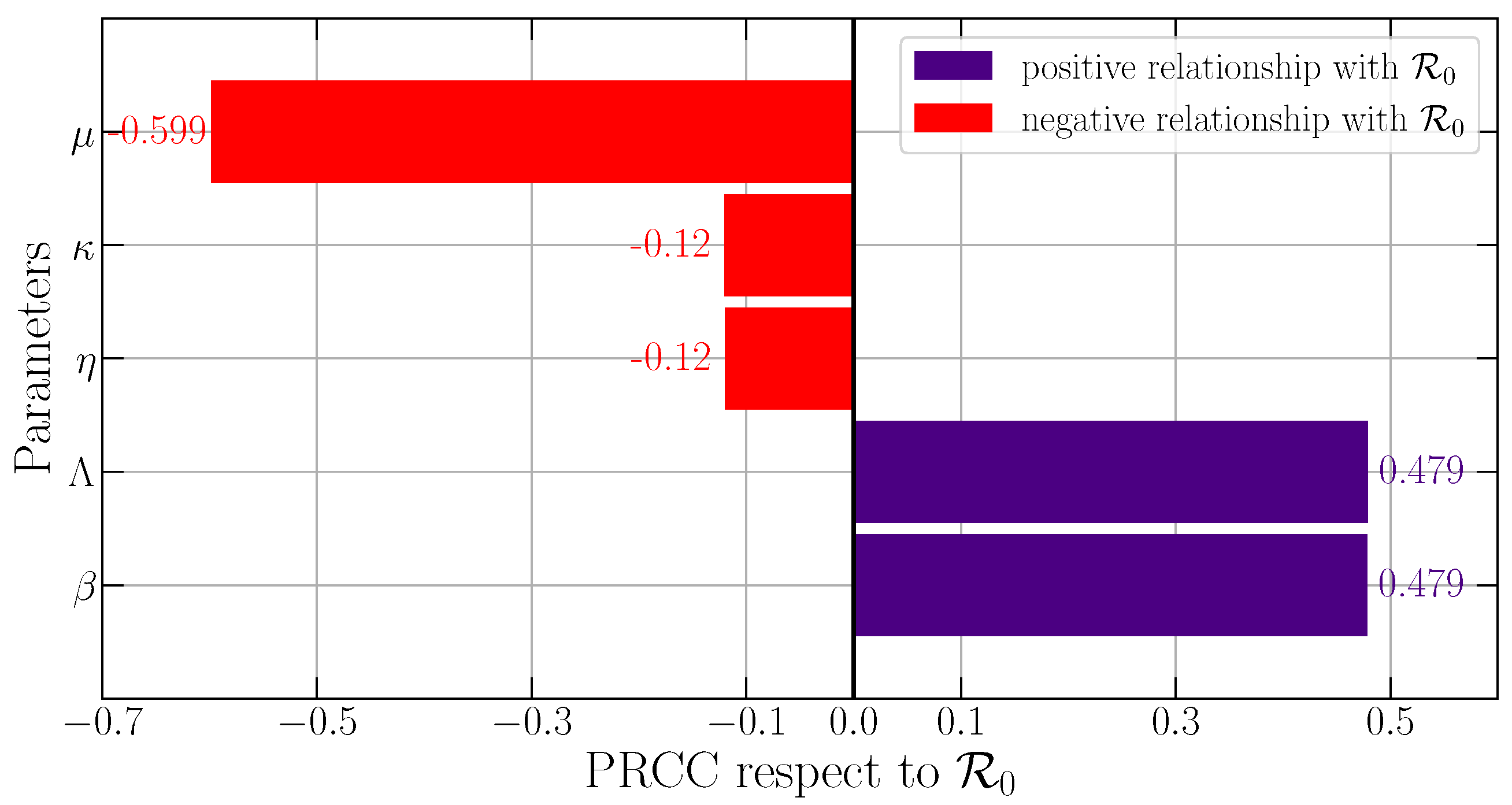
For PRCC with respect to ${\mathcal{R}}_0$, the result is provided by Figure 2. We can see that μ, κ, and η have negative relationships with ${\mathcal{R}}_0$ while Λ and β have positive relationships with ${\mathcal{R}}_0$. This means that the value of ${\mathcal{R}}_0$ decreases when μ, κ, and η increase, and the value of ${\mathcal{R}}_0$ increases when Λ and β increase. Furthermore, we find that the natural death rate (μ) becomes the first influential parameter with PRCC of $\mu =-0.599$. The second influential parameter is provided by the birth rate of susceptible prey (Λ) and the intraspecific disease transmission rate on prey (β) with PRCC of $\Lambda =\beta =0.479$. Since the birth and natural death rates are biologically fixed in nature, we conclude that β is the most influential parameter with respect to ${\mathcal{R}}_0$.

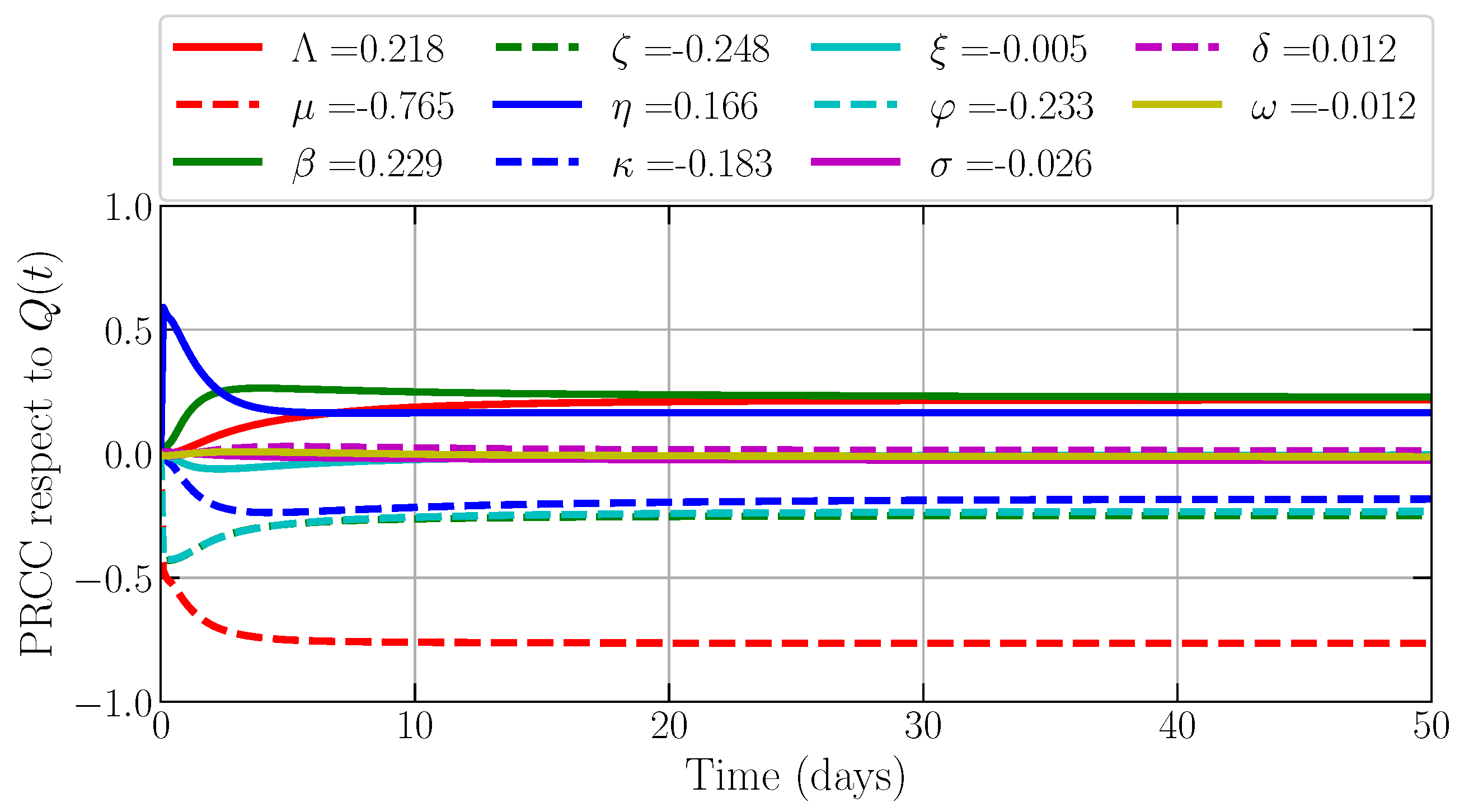
For investigating the most influential parameter regarding the density for each compartment, we also ignore the values of Λ, μ, δ, κ, and φ for the similar reason as above, where birth and death rate are fixed. We also simulate the PRCC for $0\le t\le 50$ and take the PRCC value at $t=50$ by considering the convergence of all PRCC values. Now, we study the most influential parameter regarding the density of susceptible prey S(t). Figure 3 shows that the transmission rate $\left(\beta \right)$ becomes the first influential parameter with PRCC values provided by $\beta =-0.115$, which means that, if β increases, then the density of S decreases. The second place is provided by the quarantine rate $\left(\eta \right)$ with the PRCC value provided by $\eta =0.064$. For infected prey (I(t)), we find that η and β still become the most influential parameters with PRCC values $\eta =-0.333$ and $\beta =0.309$; see Figure 4. Next, Figure 5 shows that the recovery rate $\left(\zeta \right)$ and the intraspecific disease transmission rate on prey $\left(\beta \right)$ become the most influential parameters to the density of quarantine prey (Q(t)), where the PRCC values are provided by $\zeta =-0.248$ and $\beta =0.229$. These also confirm that $\beta$ is directly and η is inversely proportional to the density of Q(t).

From all numerical simulations for global sensitivity analysis,

Table 1. Interpretation of global sensitivity analysis.

Objective Functions	Most Influential Parameter	Biological Interpretation
${\mathcal{R}}_0$	$\beta$	The disease transmission rate has the greatest influence on increasing or decreasing the basic reproduction number. The disease transmission rate is directly proportional to basic reproduction number.
$S\left(t\right)$	$\beta$	The disease transmission rate has the greatest influence on increasing or decreasing the density of the susceptible prey. The disease transmission rate is inversely proportional to the density of the susceptible prey.
$I\left(t\right)$	$\eta$	The quarantine rate has the greatest influence on increasing or decreasing the density of the infected prey. The quarantine rate is inversely proportional to the density of the infected prey.
$Q\left(t\right)$	$\zeta$	The recovery rate has the greatest influence on increasing or decreasing the density of the quarantine prey. The recovery rate is inversely proportional to the density of the quarantine prey.

is provided to describe the most influential parameters and their impact on the model. Since the birth rate and death rate are naturally possessed by every population, we assume these parameters are fixed in nature and focus on investigating the other parameters.

4.2. Dynamical Behaviors

In this subsection, we explore more the dynamical behaviors of model (3) by providing some numerical simulations based on a predictor–corrector approach developed by Diethelm et al. [63]. Three important biological parameters are investigated, namely the intraspecific disease transmission rate on prey $\left(\beta \right)$, quarantine rate on prey $\left(\eta \right)$, and the memory effect $\left(\alpha \right)$. Since we do not study a specific ecological case, all parameter values are experimentally determined. All simulations are provided based on the following parameter values.

$$\begin{array}{cccccccccccccccccc}\Lambda & =& 0.6,\hfill & \mu & =& 0.1,\hfill & \beta & =& 0.1,\hfill & \zeta & =& 0.3,\hfill & \eta & =& 0.2,\hfill & \kappa & =& 0.2,\hfill \\ \xi & =& 0.3,\hfill & \phi & =& 0.1,\hfill & \sigma & =& 0.2,\hfill & \delta & =& 0.1,\hfill & \omega & =& 0.1,\hfill & \alpha & =& 0.9.\hfill \end{array}$$

(23)

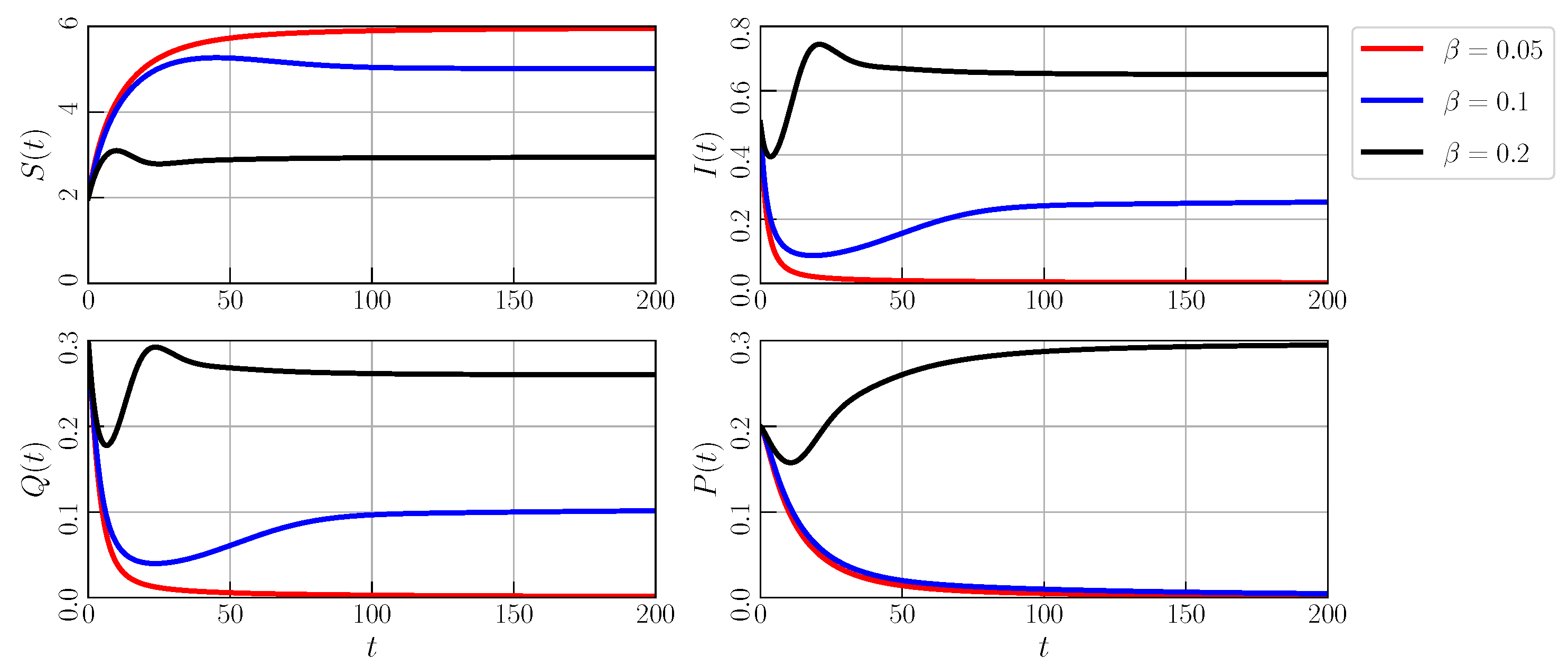
Now, to study the influence of the intraspecific disease transmission rate on prey, we vary $\beta$ in interval $[0,0.3]$. The stability and the occurrence of each equilibrium point are provided in Figure 6. For $0\le \beta <{\beta }_1^{*}\approx 0.083({\mathcal{R}}_0\approx 1)$, only an asymptotically stable PDFP ${\mathcal{E}}_1$ occurs. The stability of ${\mathcal{E}}_1$ is lost and an asymptotically stable PFEP ${\mathcal{E}}_2$ occurs when $\beta$ crosses ${\beta }_1^{*}$ via forward bifurcation. The PDFP is still unstable until $\beta =0.3$. When we do continue to the other branch, the stability of ${\mathcal{E}}_2$ holds for ${\beta }_1^{*}<\beta <{\beta }_2^{*}({\mathcal{R}}_0\approx 1.463)$. When $\beta$ crosses ${\beta }_2^{*}\approx 1.463$, the PFEP ${\mathcal{E}}_2$ also losses its stability via forward bifurcation marked by the appearance of an asymptotically stable PEP ${\mathcal{E}}_3$ simultaneously. This condition holds for ${\beta }_2^{*}<\beta \le 0.3$. To provide more description about these conditions, the time series is provided in Figure 7. We choose values of $\beta$ based on the three intervals above. For $\beta =0.05$, only susceptible prey (S) could maintain its existence while others are going to the extinction point. For $\beta =0.1$, the predator still goes to the extinction point, while the infected (I) and quarantine Q exist. This means that the disease will become endemic without the existence of a predator. When we set $\beta =0.2$, all compartments of prey and predator become existent. If we consider the dynamics according to basic reproduction number $\left({\mathcal{R}}_0\right)$, the prey not only becomes free from disease but also free from the predator when ${\mathcal{R}}_0<1$. When $1<{\mathcal{R}}_0⪅1.463$, the disease becomes endemic but the predator will be extinct. The density of all compartments exists and is balanced in nature when ${\mathcal{R}}_0>1.463$.

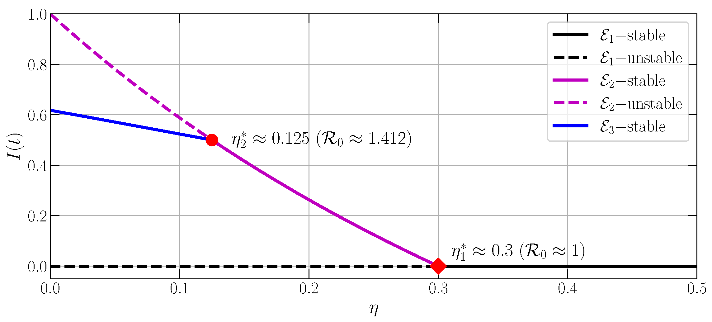
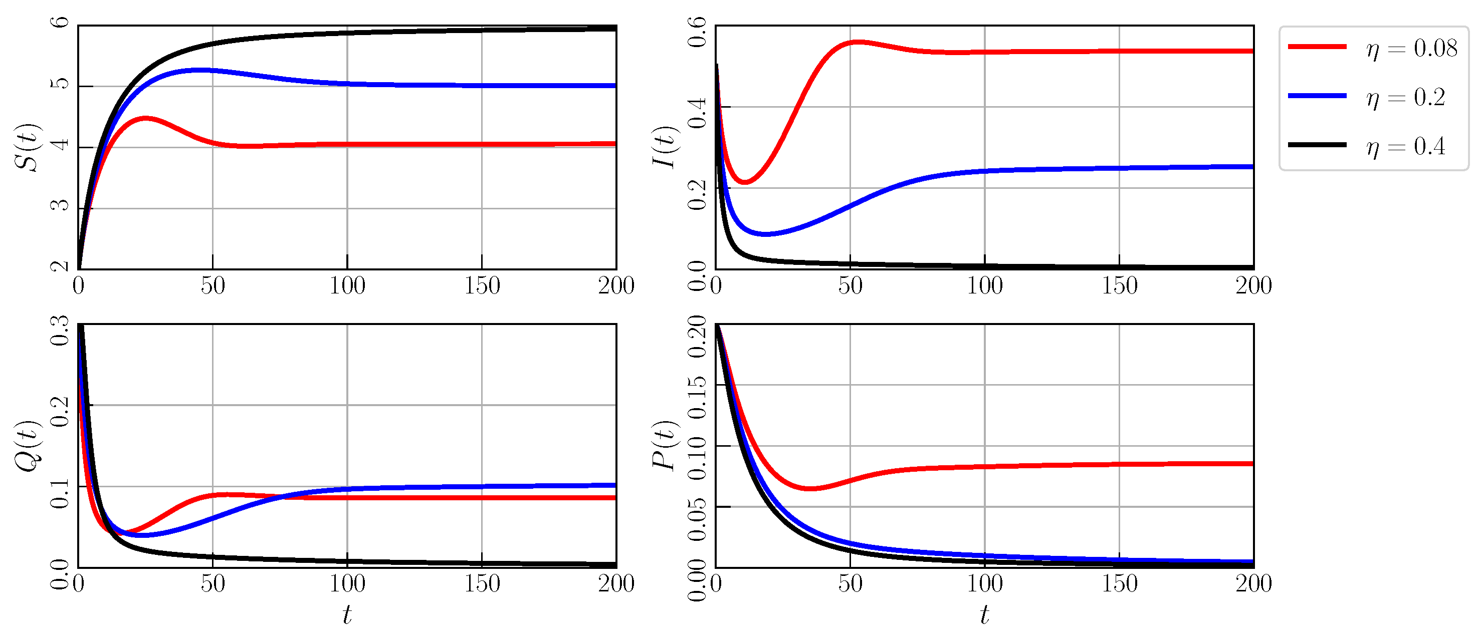
Furthermore, by still using parameter values as in Equation (23), we now study the influence of the quarantine rate on prey $\left(\eta \right)$ on the population dynamics. The parameter $\eta$ is varied in inteval $[0,0.5]$. As a result, we have Figure 8 as the bifurcation diagram. For $0\le \eta <{\eta }_2^{*}\approx 0.125({\mathcal{R}}_0\approx 1.412)$, all equilibrium points exist but only PEP ${\mathcal{E}}_3$ is asymptotically stable. The PEP ${\mathcal{E}}_3$ merges with unstable PFEP ${\mathcal{E}}_2$ when $\eta ={\eta }_2^{*}$. When $\eta$ passes through ${\eta }_2^{*}$, ${\mathcal{E}}_3$ vanishes and ${\mathcal{E}}_2$ becomes asymptotically stable via forward bifurcation. In a similar manner, PEFP ${\mathcal{E}}_2$ also merges with an unstable PDFP ${\mathcal{E}}_1$ when $\eta ={\eta }_1^{*}\approx 0.3({\mathcal{R}}_0\approx 1)$ and dissapears when $\eta >{\eta }_1^{*}$. The PDFP ${\mathcal{E}}_1$ becomes asymptotically stable via forward bifurcation when $\eta$ crosses ${\eta }_1^{*}$. Generally, if $0<\eta <{\eta }_2^{*}({\mathcal{R}}_0>1.412)$, then all compartments exist; if ${\eta }_2^{*}<\eta <{\eta }_1^{*}(1<{\mathcal{R}}_0<1.412)$, then disease becomes endemic and the predator extinct, and, if $\eta >{\eta }_1^{*}({\mathcal{R}}_0<1)$, then disease disappears from prey and the predator becomes extinct. In Figure 9, we provide the time series of model (3) using parameter values (23) and $\eta =0.08,0.2,0.4$, which represent the dynamics for each interval.

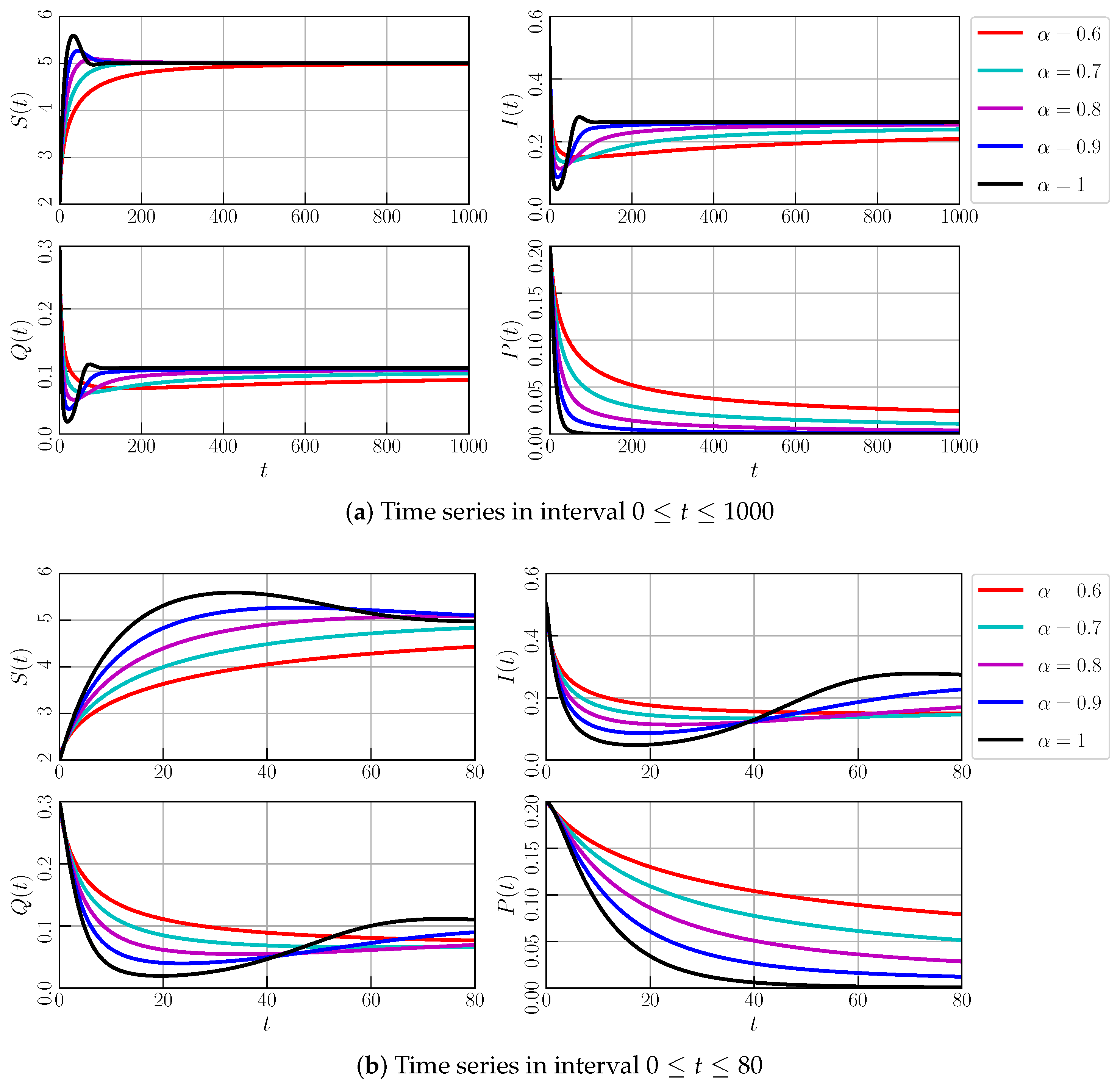
Finally, we investigate the impact of the memory effect on the dynamics of model (3). By using the parameter values from Equation (23), we vary the order of the derivative $\left(\alpha \right)$ as the memory index. We set $\alpha =$ 0.6, 0.7, 0.8, 0.9, 1 and portray them in the time series provided by Figure 10. We confirm that, when $\alpha$ is varied, all solutions seem to converge to the same equilibrium point. The difference lies in the convergence rate, where, for smaller $\alpha$, the convergence rate is also lower. This means that the memory affects the convergence rate of all compartments. These conditions are provided by Figure 10a. Furthermore, in Figure 10b, we find that $\alpha =1$ has the highest peak for S(t), I(t), and Q(t) and lowest density for P(t). This means that the memory has an impact to the maximum density of all compartments.

5. Conclusions

The dynamics of a fractional order eco-epidemiological model with quarantine have been investigated. The validity of the model has been proven by showing that the solution always exists and is unique as well as always non-negative and bounded when the initial condition is non-negative. Three feasible equilibrium points have been founded, namely the predator-disease-free, the predator-free-endemic, and the predator-endemic points. The basic reproduction number has been obtained after investigating the condition when the prey population is free from disease and predator hunting. The local and global dynamics of each equilibrium point have been identified using Matignon’s condition, Lyapunov direct method, and LaSallee invariant principle. Some numerical simulations have been demonstrated. A PRCC has been utilized to identify the most influential parameter to the value of the basic reproduction number and the density of each compartment. A pair of forward bifurcations occur when some parameters are varied, including their time series. All analytical and numerical simulations show that intraspecific disease transmission and the quarantine rate provide the most contribution to the density of the infected prey population. This means that we have to increase the intraspecific disease transmission and increase the quarantine rate to suppress the disease as well as maintain the ecological balance.

References

1. Anderson, R.M.; May, R.M.; Joysey, K.; Mollison, D.; Conway, G.R.; Cartwell, R.; Thompson, H.V.; Dixon, B. The Invasion, Persistence and Spread of Infectious Diseases within Animal and Plant Communities. Philos. Trans. R. Soc. B Biol. Sci. 1986, 314, 533–570. [Google Scholar] [CrossRef]
2. Chattopadhyay, J.; Arino, O. A predator-prey model with disease in the prey. Nonlinear Anal. Theory Methods Appl. 1999, 36, 747–766. [Google Scholar] [CrossRef]
3. Venturino, E. Epidemics in predator–prey models: Disease in the predators. J. Math. Appl. Med. Biol. 2002, 19, 185–205. [Google Scholar] [CrossRef]
4. Siekmann, I. On competition in ecology, epidemiology and eco-epidemiology. Ecol. Complex. 2013, 14, 166–179. [Google Scholar] [CrossRef]
5. Rahmi, E.; Darti, I.; Suryanto, A.; Trisilowati, T. A Fractional-Order Eco-Epidemiological Leslie–Gower Model with Double Allee Effect and Disease in Predator. Int. J. Differ. Equ. 2023, 2023, 5030729. [Google Scholar] [CrossRef]
6. Naji, R.K.; Mustafa, A.N. The Dynamics of an Eco-Epidemiological Model with Nonlinear Incidence Rate. J. Appl. Math. 2012, 2012, 852631. [Google Scholar] [CrossRef]
7. Rahman, M.S.; Chakravarty, S. A predator-prey model with disease in prey. Nonlinear Anal. Model. Control 2013, 18, 191–209. [Google Scholar] [CrossRef] [Green Version]
8. Kant, S.; Kumar, V. Dynamics of a prey-predator system with infection in prey. Electron. J. Differ. Equ. 2017, 2017, 1–27. [Google Scholar]
9. Greenhalgh, D.; Khan, Q.J.A.; Al-kharousi, F.A. Eco-epidemiological model with fatal disease in the prey. Nonlinear Anal. Real World Appl. 2020, 53, 103072. [Google Scholar] [CrossRef]
10. Moustafa, M.; Mohd, M.H.; Ismail, A.I.; Abdullah, F.A. Dynamical analysis of a fractional-order eco-epidemiological model with disease in prey population. Adv. Differ. Equ. 2020, 2020. [Google Scholar] [CrossRef] [Green Version]
11. Lopez, L.K.; Cortez, M.H.; Deblieux, T.S.; Hall, S.R.; Menel, I.A.; Brien, B.O.; Carla, E.C.; Duffy, M.A. A healthy but depleted herd: Predators decrease prey disease and density. Ecology 2023, 104, e4063. [Google Scholar] [CrossRef]
12. Mbava, W.; Mugisha, J.Y.T.; Gonsalves, J.W. Prey, Predator and Super-Predator Model with Disease in the Super-Predator. Appl. Math. Comput. 2017, 297, 92–114. [Google Scholar] [CrossRef]
13. Bate, A.M.; Hilker, F.M. Complex Dynamics in an Eco-epidemiological Model. Bull. Math. Biol. 2013, 75, 2059–2078. [Google Scholar] [CrossRef] [PubMed]
14. Kang, A.; Xue, Y.; Fu, J. Dynamic Behaviors of a Leslie-Gower Ecoepidemiological Model. Discret. Dyn. Nat. Soc. 2015, 2015, 169242. [Google Scholar] [CrossRef] [Green Version]
15. Shaikh, A.A.; Das, H.; Ali, N. Study of LG-Holling type III predator–prey model with disease in predator. J. Appl. Math. Comput. 2018, 58, 235–255. [Google Scholar] [CrossRef] [Green Version]
16. Mondal, A.; Pal, A.K.; Samanta, G.P. On the dynamics of evolutionary Leslie-Gower predator-prey eco-epidemiological model with disease in predator. Ecol. Genet. Genom. 2019, 10, 100034. [Google Scholar] [CrossRef]
17. Herrera, J.; Nunn, C.L. Behavioural ecology and infectious disease: Implications for conservation of biodiversity. Philos. Trans. R. Soc. B Biol. Sci. 2019, 374, 20180054. [Google Scholar] [CrossRef] [Green Version]
18. Perumal, R.; Munigounder, S.; Mohd, M.H.; Balachandran, K. Stability analysis of the fractional-order prey-predator model with infection. Int. J. Model. Simul. 2021, 41, 434–450. [Google Scholar] [CrossRef]
19. Bhattacharjee, D.; Kashyap, A.J.; Sarmah, H.K.; Paul, R. Dynamics in a ratio-dependent eco-epidemiological predator-prey model having cross species disease transmission. Commun. Math. Biol. Neurosci. 2021, 2021, 15. [Google Scholar] [CrossRef]
20. pada Das, K. A study of harvesting in a predator—Prey model with disease in both populations. Math. Methods Appl. Sci. 2016, 39, 2853–2870. [Google Scholar] [CrossRef]
21. Sharma, S.; Samanta, G.P. A Leslie-Gower predator-prey model with disease in prey incorporating a prey refuge. Chaos Solitons Fractals 2015, 70, 69–84. [Google Scholar] [CrossRef]
22. Wang, S.; Ma, Z.; Wang, W. Dynamical behavior of a generalized eco-epidemiological system with prey refuge. Adv. Differ. Equ. 2018, 2018, 244. [Google Scholar] [CrossRef]
23. Bhattacharyya, R.; Mukhopadhyay, B. On an Eco-Epidemiological Model with Prey Harvesting and Predator Switching: Local and Global Perspectives. Nonlinear Anal. Real World Appl. 2010, 11, 3824–3833. [Google Scholar] [CrossRef]
24. Meng, X.Y.; Qin, N.N.; Huo, H.F. Dynamics analysis of a predator–prey system with harvesting prey and disease in prey species. J. Biol. Dyn. 2018, 12, 342–374. [Google Scholar] [CrossRef]
25. Cojocaru, M.; Migot, T.; Jaber, A. Controlling infection in predator-prey systems with transmission dynamics. Infect. Dis. Model. 2020, 5, 1–11. [Google Scholar] [CrossRef]
26. Bezabih, A.F.; Edessa, G.K.; Rao, K.P. Ecoepidemiological Model and Analysis of Prey-Predator System. J. Appl. Math. 2021, 2021, 6679686. [Google Scholar] [CrossRef]
27. Kang, Y.; Kumar Sasmal, S.; Ranjan Bhowmick, A.; Chattopadhyay, J. Dynamics of a predator-prey system with prey subject to Allee effects and disease. Math. Biosci. Eng. 2014, 11, 877–918. [Google Scholar] [CrossRef]
28. Saifuddin, M.; Biswas, S.; Samanta, S.; Sarkar, S.; Chattopadhyay, J. Complex dynamics of an eco-epidemiological model with different competition coefficients and weak Allee in the predator. Chaos Solitons Fractals 2016, 91, 270–285. [Google Scholar] [CrossRef]
29. Wang, L.; Qiu, Z.; Feng, T.; Kang, Y. An eco-epidemiological model with social predation subject to a component Allee effect. Appl. Math. Model. 2022, 101, 111–131. [Google Scholar] [CrossRef]
30. Babaei, A.; Ahmadi, M.; Jafari, H.; Liya, A. A mathematical model to examine the effect of quarantine on the spread of coronavirus. Chaos Solitons Fractals 2021, 142, 33–37. [Google Scholar] [CrossRef]
31. Shah, N.H.; Sheoran, N.; Jayswal, E. Z-Control on COVID-19-Exposed Patients in Quarantine. Int. J. Differ. Equ. 2020, 2020. [Google Scholar] [CrossRef]
32. Aronna, M.S.; Guglielmi, R.; Moschen, L.M. A model for COVID-19 with isolation, quarantine and testing as control measures. Epidemics 2021, 34, 100437. [Google Scholar] [CrossRef]
33. Farman, M.; Akgül, A.; Fahad Aldosary, S.; Nisar, K.S.; Ahmad, A. Fractional order model for complex Layla and Majnun love story with chaotic behaviour. Alex. Eng. J. 2022, 61, 6725–6738. [Google Scholar] [CrossRef]
34. Coronel-Escamilla, A.; Gómez-Aguilar, J.; López-López, M.; Alvarado-Martínez, V.; Guerrero-Ramírez, G. Triple pendulum model involving fractional derivatives with different kernels. Chaos Solitons Fractals 2016, 91, 248–261. [Google Scholar] [CrossRef]
35. Almeida, R.; Brito da Cruz, A.M.; Martins, N.; Monteiro, M.T.T. An epidemiological MSEIR model described by the Caputo fractional derivative. Int. J. Dyn. Control. 2019, 7, 776–784. [Google Scholar] [CrossRef] [Green Version]
36. Chen, S.B.; Jahanshahi, H.; Alhadji Abba, O.; Solís-Pérez, J.E.; Bekiros, S.; Gómez-Aguilar, J.F.; Yousefpour, A.; Chu, Y.M. The effect of market confidence on a financial system from the perspective of fractional calculus: Numerical investigation and circuit realization. Chaos Solitons Fractals 2020, 140, 110223. [Google Scholar] [CrossRef]
37. Acay, B.; Inc, M. Fractional modeling of temperature dynamics of a building with singular kernels. Chaos Solitons Fractals 2021, 142, 110482. [Google Scholar] [CrossRef]
38. Srivastava, H.M.; Dubey, V.P.; Kumar, R.; Singh, J.; Kumar, D.; Baleanu, D. An efficient computational approach for a fractional-order biological population model with carrying capacity. Chaos Solitons Fractals 2020, 138, 109880. [Google Scholar] [CrossRef]
39. Barman, D.; Roy, J.; Alam, S. Modelling hiding behaviour in a predator-prey system by both integer order and fractional order derivatives. Ecol. Inform. 2022, 67, 101483. [Google Scholar] [CrossRef]
40. Abdullah, F.A.; Moustafa, M.; Ismail, A.I.; Mohd, M.H. Global stability of a fractional order eco-epidemiological system with infected prey. Int. J. Math. Model. Numer. Optim. 2021, 11, 53. [Google Scholar] [CrossRef]
41. Ogunrinde, R.B.; Nwajeri, U.K.; Fadugba, S.E.; Ogunrinde, R.R.; Oshinubi, K.I. Dynamic model of COVID-19 and citizens reaction using fractional derivative. Alex. Eng. J. 2021, 60, 2001–2012. [Google Scholar] [CrossRef]
42. Djilali, S.; Ghanbari, B. The influence of an infectious disease on a prey-predator model equipped with a fractional-order derivative. Adv. Differ. Equ. 2021, 2021, 20. [Google Scholar] [CrossRef]
43. Jurczynski, K.; Lyashchenko, K.P.; Gomis, D.; Journal, S.; Medicine, W.; June, N. Pinniped Tuberculosis In Malayan Tapirs (Tapirus indicus) and Its Transmission to Other Terrestrial Mammals. J. Zoo Wildl. Med. 2011, 42, 222–227. [Google Scholar] [CrossRef]
44. Martin, C.; Pastoret, P.P.; Brochier, B.; Humblet, M.F.; Saegerman, C. A survey of the transmission of infectious diseases/infections between wild and domestic ungulates in Europe. Vet. Res. 2011, 42, 70. [Google Scholar] [CrossRef] [PubMed] [Green Version]
45. Woodford, M.H. Quarantine and Health Screening Protocols for Wildlife Prior to Translocation and Release into the Wild; IUCN Species Survival Commission’s Veterinary Specialist Group, Gland, the Office International des Epizooties (OIE), Paris, Care for the Wild and the European Association of Zoo and Wildlife Veterinarians. 2000. Available online: https://digitalcommons.unl.edu/zoonoticspub/32/ (accessed on 20 February 2023).
46. Petras, I. Fractional-Order Nonlinear Systems: Modeling, Analysis and Simulation; Springer: Berlin, Heidelberg, 2011. [Google Scholar] [CrossRef] [Green Version]
47. Poria, S.; Dhiman, A. Existence and uniqueness of solution to ODEs: Lipschitz continuity. Resonance 2017, 22, 491–507. [Google Scholar] [CrossRef]
48. Podlubny, I. Fractional Differential Equations; Academic Press: London, UK, 1999. [Google Scholar]
49. Cresson, J.; Szafrańska, A. Discrete and continuous fractional persistence problems—The positivity property and applications. Commun. Nonlinear Sci. Numer. Simul. 2017, 44, 424–448. [Google Scholar] [CrossRef] [Green Version]
50. Anbalagan, P.; Hincal, E.; Ramachandran, R.; Baleanu, D.; Cao, J.; Niezabitowski, M. A Razumikhin approach to stability and synchronization criteria for fractional order time delayed gene regulatory networks. AIMS Math. 2021, 6, 4526–4555. [Google Scholar] [CrossRef]
51. Choi, S.K.; Kang, B.; Koo, N. Stability for Caputo Fractional Differential Systems. Abstr. Appl. Anal. 2014, 2014, 631419. [Google Scholar] [CrossRef] [Green Version]
52. Matignon, D. Stability results for fractional differential equations with applications to control processing. In Proceedings of the CESA’96 IMACS Multiconference: Computational Engineering in Systems Applications, Lille, France, 9–12 July 1996; Volume 2, pp. 963–968. [Google Scholar]
53. Huo, J.; Zhao, H.; Zhu, L. The effect of vaccines on backward bifurcation in a fractional order HIV model. Nonlinear Anal. Real World Appl. 2015, 26, 289–305. [Google Scholar] [CrossRef]
54. Okyere, S.; Ackora-Prah, J. Modeling and analysis of monkeypox disease using fractional derivatives. Results Eng. 2023, 17, 100786. [Google Scholar] [CrossRef]
55. Peter, O.J.; Panigoro, H.S.; Abidemi, A.; Ojo, M.M.; Oguntolu, F.A. Mathematical Model of COVID-19 Pandemic with Double Dose Vaccination. Acta Biotheor. 2023, 71, 9. [Google Scholar] [CrossRef] [PubMed]
56. Peter, O.J.; Panigoro, H.S.; Ibrahim, M.A.; Otunuga, O.M.; Ayoola, T.A.; Oladapo, A.O. Analysis and dynamics of measles with control strategies: A mathematical modeling approach. Int. J. Dyn. Control 2023. [Google Scholar] [CrossRef]
57. Diekmann, O.; Heesterbeek, J.; Metz, J. On the definition and the computation of the basic reproduction ratio R 0 in models for infectious diseases in heterogeneous populations. J. Math. Biol. 1990, 28, 365–382. [Google Scholar] [CrossRef] [Green Version]
58. Sinan, M.; Shah, K.; Kumam, P.; Mahariq, I.; Ansari, K.J.; Ahmad, Z.; Shah, Z. Fractional order mathematical modeling of typhoid fever disease. Results Phys. 2022, 32, 105044. [Google Scholar] [CrossRef]
59. Anggriani, N.; Beay, L.K. Modeling of COVID-19 spread with self-isolation at home and hospitalized classes. Results Phys. 2022, 36, 105378. [Google Scholar] [CrossRef]
60. Vargas-De-León, C. Volterra-type Lyapunov functions for fractional-order epidemic systems. Commun. Nonlinear Sci. Numer. Simul. 2015, 24, 75–85. [Google Scholar] [CrossRef]
61. Ahmed, E.; El-Sayed, A.; El-Saka, H.A. On some Routh–Hurwitz conditions for fractional order differential equations and their applications in Lorenz, Rössler, Chua and Chen systems. Phys. Lett. A 2006, 358, 1–4. [Google Scholar] [CrossRef]
62. Pratap, A.; Raja, R.; Agarwal, R.P.; Alzabut, J.; Niezabitowski, M.; Hincal, E. Further results on asymptotic and finite-time stability analysis of fractional-order time-delayed genetic regulatory networks. Neurocomputing 2022, 475, 26–37. [Google Scholar] [CrossRef]
63. Diethelm, K.; Ford, N.J.; Freed, A.D. A Predictor-Corrector Approach for the Numerical Solution of Fractional Differential Equations. Nonlinear Dyn. 2002, 29, 3–22. [Google Scholar] [CrossRef]
64. Marino, S.; Hogue, I.B.; Ray, C.J.; Kirschner, D.E. A methodology for performing global uncertainty and sensitivity analysis in systems biology. J. Theor. Biol. 2008, 254, 178–196. [Google Scholar] [CrossRef] [Green Version]
65. Saltelli, A. Making best use of model evaluations to compute sensitivity indices. Comput. Phys. Commun. 2002, 145, 280–297. [Google Scholar] [CrossRef]
66. Saltelli, A.; Annoni, P.; Azzini, I.; Campolongo, F.; Ratto, M.; Tarantola, S. Variance based sensitivity analysis of model output. Design and estimator for the total sensitivity index. Comput. Phys. Commun. 2010, 181, 259–270. [Google Scholar] [CrossRef]
67. Herman, J.; Usher, W. SALib: An open-source Python library for Sensitivity Analysis. J. Open Source Softw. 2017, 2, 97. [Google Scholar] [CrossRef]
Figure 1. The food chain and compartmental diagram of eco-epidemiological model.
Fractalfract 07 00610 g001
Figure 2. PRCC of parameters of model (3) with respect to the basic reproduction number R 0 .
Fractalfract 07 00610 g002
Figure 3. PRCC of parameters of model (3) with respect to the susceptible prey S(t).
Fractalfract 07 00610 g003
Figure 4. PRCC of parameters of model (3) with respect to the infected prey I(t).
Fractalfract 07 00610 g004
Figure 5. PRCC of parameters of model (3) with respect to the quarantine prey Q(t).
Fractalfract 07 00610 g005
Figure 6. Bifurcation diagram of model (3) driven by β with parameter values provided by Equation (23).
Fractalfract 07 00610 g006
Figure 7. Time series of model (3) for β = 0.05, 0.1, and 0.2 with parameter values provided by Equation (23).
Fractalfract 07 00610 g007
Figure 8. Bifurcation diagram of model (3) driven by η with parameter values provided by Equation (23).
Fractalfract 07 00610 g008
Figure 9. Time series of model (3) for η = 0.08, 0.2, and 0.4 with parameter values provided by Equation (23).
Fractalfract 07 00610 g009
Figure 10. Time series of model (3) with experimental parameter values as follows: Λ = 0.6 , μ = 0.1 , β = 0.1 , ζ = 0.3 , η = 0.2 , κ = 0.2 , ξ = 0.3 , φ = 0.1 , σ = 0.2 , δ = 0.1 , and ω = 0.1 .
Fractalfract 07 00610 g010