An Image-Denoising Framework Using ℓ_q Norm-Based Higher Order Variation and Fractional Variation with Overlapping Group Sparsity

Abstract

As one of the most significant issues in imaging science, image denoising plays a major role in plenty of image processing applications. Due to the ill-posed nature of image denoising, total variation regularization is widely used in image denoising problems for its capability to suppress noise and preserve image edges. Nevertheless, traditional total variation will inevitably yield undesirable staircase artifacts when applied to recorded images. Inspired by the success of ℓ_q norm minimization and overlapping group sparsity in image denoising, and the effective staircase artifacts removal by fractional total variation, the hybrid model which combines the fractional order total variation with overlapping group sparsity and higher order total variation with ℓ_q norm is developed in this paper to restore images corrupted by Gaussian noise. An efficient algorithm based on the parallel linear alternating direction method of multipliers is developed for solving the corresponding model and the numerical experiments demonstrate the effectiveness of the proposed approach against several state-of-the-art methods, in terms of peak signal-to-noise ratio and structure similarity index measure values.

1. Introduction

As a momentous channel for human beings to obtain external information, the image plays an increasingly important role in modern society. However, due to the imperfection of image acquisition, conversion and transmission systems, the image quality may be inevitably degraded to varying degrees. Noises in the image degradation process not only affect the visual effect of the image, but also mask important feature information in the image, which will bring difficulties to the subsequent processing of the image. Consequently, it is of great significance to research the image-denoising technology.

The image-degradation process can be modeled as the following linear system:

$$f=Hu+\eta$$

(1)

where f is the blurred and noisy image with the size of M × N, u denotes the original clean image to be estimated, H represents the blurring operator known as the point spread function and $\eta$ is an additive noise.

Mathematically, image denoising belongs to a class of inverse problems [1,2], most of which are ill-posed. The aim of image denoising is to approximately recover the true image u from the observed image f and it is generally accepted that the regularization method is effective for reducing ill-posedness and obtaining stable and accurate solutions. One of the commendable regularization methods is Thikhonov regularization, since it has the advantage of simple calculations; nevertheless, it tends to make images overly smoothed so that important image attributes, such as sharp edges, often fail to be adequately preserved. In order to overcome this shortcoming, Rudin, Osher and Fatemi proposed the canonical ROF model [3], based on nonlinear total variation (TV) regularization. The image denoising problem with regularization is usually modeled as the following form of functional minimization problem:

$$\underset{u}{\min }J(Hu,f)+\lambda \phi (u)$$

(2)

where $J(Hu,f)$ is the fidelity term that describes the similarity between the observed image and the latent image according to model (1), and its specific form depends on the type of noise in the observed image. $\phi (u)$ denotes the regularization term, which typically models desirable prior properties of the image, such as smoothness, sharp edges, contrast and so on, and plays a role in suppressing noise, smoothing results and stabilizing numerical values. $\lambda >0$ is the regularization parameter which controls the trade-off between the regularization term and the fidelity term.

Numerous effective optimization algorithms have been developed for solving problem (2), including the primal-dual algorithm [4,5,6], splitting Bregman algorithm [7,8,9], the alternating direction method of multipliers (ADMM) [10,11,12] and so on. To process massive and high-quality images better, a powerful, flexible, and parallel algorithm is the focus for solving image inverse problems. Developing parallel splitting methods and combining them with distributed computing to address image big data problems will be a hot topic of academic research for a long time in the future.

Although TV regularization has been proven to be extraordinarily useful in plenty of applications, traditional TV tends to yield staircase artifacts, causing piecewise constant approximation of the true image in bounded variation space. To avoid these drawbacks, varieties of improved regularization methods have been introduced, such as higher order TV [13,14,15,16], generalized TV [17,18,19], non-local TV [20,21,22], fractional order TV [23,24,25,26,27], non-convex TV [28,29,30] and so on. As a generalization of integer order calculus, the fractional order calculus has been successfully applied to image denoising in recent years, due to its nonlocal property, which can avoid over-smoothing at edges and preserve the detailed information of images. By utilizing the fractional order derivatives to represent image features, the following convex variational model was proposed by Mei et al. [27] for image denoising:

$$\underset{u}{min}{\displaystyle {\int }_{\Omega }|Du|+\frac{\alpha }{2}}{\displaystyle {\int }_{\Omega }|D^{\gamma }u-w{|}^2}dx+\frac{\beta }{2}{\displaystyle {\int }_{\Omega }|u-u_0{|}^2}dx$$

(3)

where $D^{\gamma }u$ denotes γ-order gradient of image u, w is the target fractional order gradient feature, and $u_0$ is a pre-defined image. Numerical experiments demonstrate that this method outperforms other traditional TV-based approaches in image denoising. Another state-of-the-art approach to deal with staircase artifacts is the hybrid model [31,32,33,34] of both classical TV regularization and other kind of regularization, which combines the advantages of single models and generally has better denoising effects than single models.

Sparse representation is currently a hot topic in the fields of signal processing, machine learning and optimization methods, and has received the widespread attention of researchers in computer vision, signal processing, computational mathematics and other fields. For instance, Peyré and Fadili [35] studied the property of overlapping group sparsity and verified the superior numerical property of overlapping group sparsity, compared to non-overlapping group sparsity, through a large number of compressed sensing experiments. The work of Slesnick et al. [36] focused on a TV denoising model for sparse regularization of one-dimensional signal overlapping groups. On this basis, Liu et al. [37] built a TV image denoising model based on overlapping group sparsity (OGS-TV). Moreover, a non-convex hybrid overlapping group sparsity model with hyper-Laplacian prior was presented in [38], which effectively eliminated multiplicative noise. Their numerical experiments demonstrated that the OGS method can alleviate the staircase artifacts effectively. In addition, the research of image restoration based on OGS regularization is still the focus of many scholars [39,40,41,42].

Inspired by the overlapping group sparsity and the effective staircase artifacts’ removal by fractional total variation, a novel hybrid model, which combines fractional total variation with overlapping sparsity and higher order total variation with ℓ_q norm, is proposed in this paper, for Gaussian noise removal, with the aim of eliminating staircase artifacts while balancing the smoothness and sharpness of the restored image. A parallel linear alternating direction method of multipliers is derived to handle the corresponding minimization problems, and the performance of our approach is compared to several state-of the-art denoising algorithms.

The main contributions of this paper can be summarized as follows:

• A hybrid model of both fractional total variation with overlapping group sparsity and higher order total variation with ℓ_q norm is presented, which is able to alleviate staircase artifacts sufficiently by exploiting the sparsity characteristics of images and the superiority of fractional calculus;
• The alternating direction method of multipliers is generalized, and a parallel linear ADMM framework is developed. By imposing different weights onto each operator and applying relaxed steps, fast convergence speed is achieved;
• The proposed method can be applied to image deblurring and other image processes, which is preferable in a broad spectrum of practical applications.

The remainder of this paper is structured as follows. Section 2 briefly provides several definitions and other related works. In Section 3, we derive an efficient algorithm for solving the considered minimization problem. Consequently, Section 4 shows the numerical experiment results of the proposed method and some other state-of-the-art approaches. Finally, conclusions are made in Section 5.

2. Preliminaries

2.1. Fractional Calculus

Fractional order calculus has been applied in image processing, although its definition is not unified up to date. The Riemann-Liouville (R-L) definition, Grünwald-Letnikov (G-L) definition and Caputo definition are the three main fractional calculus definitions.

Definition 1. 

Three definitions of fractional calculus.

(i) The α-order fractional calculus defined by R-L is of the form

$${}_{a}D_b^{\alpha }f(x)=\frac{d^n}{d{x}^n}\frac{1}{\mathsf{\Gamma }(n-\alpha )}{\displaystyle {\int }_a^b\frac{f(z)}{{(x-z)}^{\alpha -n+1}}}dz,0\le n-1<\alpha <n$$

(4)

where  $\mathsf{\Gamma }(x)$ is the Gamma function defined by $\mathsf{\Gamma }(x)={\displaystyle {\int }_0^{+\infty }{t}^{x-1}}{e}^{-t}dt$.

(ii) The α-order G-L fractional calculus of function $f(x)$ on the interval $[a,b]$ is defined as

$${}_{a}D_b^{\alpha }f(x)=\underset{h\to 0}{\lim }\frac{1}{h^{\alpha }}{\displaystyle \sum _{j=0}^{[(b-a)/h]}{(-1)}^j\frac{\mathsf{\Gamma }(\alpha +1)}{j!\mathsf{\Gamma }(\alpha -j+1)}}f(x-jh)$$

(5)

where$\mathsf{\Gamma }(x)$ is the Gamma function and [a] denotes the integer part of a.

(iii) Caputo definition of α-order fractional calculus is

$${}_{a}D_b^{\alpha }f(x)=\frac{d^n}{d{x}^n}\frac{1}{\mathsf{\Gamma }(n-\alpha )}{\displaystyle {\int }_a^b\frac{f^n(y)}{{(x-y)}^{\alpha -n+1}}}dy,0\le n-1<\alpha <n$$

(6)

Compared with the other two definitions, the G-L definition is more suitable for image processing since the fractional calculus takes more characteristics of proximity into consideration and is more similar to the optical imaging principle. As a result, the G-L definition is more capable of avoiding staircase artifacts and is adopted in this paper for problem solving. Let the size of the image u be M × N. Thus, the discrete form of the fractional order gradient can be calculated by:

$${({\nabla }^{\alpha }u)}_{i,j}=({({\nabla }_x^{\alpha }u)}_{i,j},{({\nabla }_y^{\alpha }u)}_{i,j}),\alpha \in {ℝ}^{+}$$

(7)

with

$$\left\{\begin{array}{c}{({\nabla }_x^{\alpha }u)}_{i,j}={\displaystyle \sum _{k=1}^{L-1}{(-1)}^k{C}_k^{\alpha }{u}_{i-k,j,}}\\ {({\nabla }_y^{\alpha }u)}_{i,j}={\displaystyle \sum _{k=1}^{L-1}{(-1)}^k{C}_k^{\alpha }{u}_{i,j-k,}}\end{array}\right.$$

(8)

for $1\le i\le M,1\le j\le N$, where $L\ge 3$ is positive integer and the generalized binominal coefficient $C_k^{\alpha }$ is given by

$$C_k^{\alpha }=\frac{\mathsf{\Gamma }(\alpha +1)}{\mathsf{\Gamma }(k+1)\mathsf{\Gamma }(\alpha -k+1)}$$

(9)

2.2. Proximity Operator

The proximity operator is a crucial concept in convex analysis and plays a significant role in solving a convex optimization model, which is closely related to the design of numerous algorithms. The proximity operator of TV was studied by Micchelli et al. [43], and a proximity algorithm for the typical TV-denoising model was developed. In this section, the definition and properties of the proximal operator associated with a closed proper convex function are briefly introduced.

Definition 2. 

Consider F to be a closed proper convex function on ${ℝ}^n$, then the proximity operator of F is defined by:

$$pro{x}_F(x)=\underset{v}{\arg \min }\{F(v)+\frac{1}{2}{‖x-v‖}_2^2\}$$

(10)

Theorem 1. 

If F is a closed and proper convex function, for any $x\in {ℝ}^n$, the value of $pro{x}_F(x)$ exists and is unique.

Example 1. 

If  $t>0$ and $x\in ℝ$ , then $pro{x}_{t|\cdot |}(x)=\max (|x|-t,0)\mathrm{sign}(x)$, where $pro{x}_{t|\cdot |}$ is a well-known soft thresholding operator with t as the threshold.

Example 2. 

If $t>0$ and $x\in ℝ$, for ℓ₁-norm ${‖x‖}_1={\displaystyle \sum _{i=1}^n\left|x_i\right|}$ and ℓ₂-norm ${‖x‖}_2=({\displaystyle \sum _{i=1}^n{x}_i^2}{)}^{{}^{\frac{1}{2}}}$, the following hold:

$$(i)pro{x}_{t{‖\cdot ‖}_1}(x)=(pro{x}_{t|\cdot |}(x_1),pro{x}_{t|\cdot |}(x_2),\dots pro{x}_{t|\cdot |}(x_n))$$

(11)

$$\mathit{(}ii\mathit{)}pro{x}_{t{‖\cdot ‖}_2}(x)=\max ({‖x‖}_2-t,0)\frac{x}{{‖x‖}_2}=pro{x}_{t|\cdot |}({‖x‖}_2)\frac{x}{{‖x‖}_2}$$

(12)

2.3. OGS-FTV

To avoid staircase artifacts produced by traditional TV regularization, an overlapping group sparsity (OGS) regularization is introduced in [37]. For the two-dimension case, the K-point group of the image $u\in {ℝ}^{n\times n}$ is given by:

$${\tilde{u}}_{i,j,K}=\left(\begin{array}{ccc}{u}_{i-n_1,j-n_1}& u_{i-n_1,j-n_1+1}\dots & u_{i-n_1,j+n_2}\\ ⋮& \ddots & ⋮\\ u_{i+n_2,j-n_1}& u_{i+n_2,j-n_1+1}\cdots & u_{i+n_2,j+n_2}\end{array}\right)\in {ℝ}^{K\times K}$$

(13)

with $n_1=\left[\frac{K-1}{2}\right],n_2=\left[\frac{K}{2}\right]$, where [x] is the greatest integer not greater than x. Let $u_{i,j,K}$ be a vector obtained by stacking the K columns of the matrix ${\tilde{u}}_{i,j,K}$ in sequence, i.e., $u_{i,j,K}={\tilde{u}}_{i,j,K}(:)$. Then, the OGS functional of u can be written as

$$\varphi (u)={\displaystyle \sum _{i=1}^n{\displaystyle \sum _{j=1}^n{‖u_{i,j,K}‖}_2}}$$

(14)

Consequently, the fractional OGS regularization functional is set to be of the form of

$$\varphi ({\nabla }_x^{\alpha }u)+\varphi ({\nabla }_y^{\alpha }u)$$

(15)

where $1<\alpha <2$ is a fraction and ${\nabla }_x^{\alpha }u,{\nabla }_y^{\alpha }u$ are the fractional order gradients of u. A fractional total variation model based on OGS can better exploit the structural sparse prior knowledge among image gradients and further reduce the staircase artifacts of commonly used TV models through the structural property of image gradients. Especially, when $K=1$, $\alpha =1$, the corresponding regularization term is commonly mentioned as a traditional anisotropic TV functional.

3. The Proposed Algorithm

3.1. Derivation of Parallel Linear ADMM

Consider the following objective function:

$$\underset{x}{\min }g(x)+{\displaystyle \sum _{j=1}^J{h}_j(T_{j}x)}$$

(16)

Denote the set of all proper and lower semicontinuous from the Hilbert space to $ℝ\cup \left\{+\infty \right\}$ as ${\mathsf{\Gamma }}_0\left\{x\right\}.$ In (16), $g\in {\mathsf{\Gamma }}_0\left\{X\right\},h_j\in {\mathsf{\Gamma }}_0\left\{V_j\right\}$, which are simple enough in the sense that the proximity operators of them possess closed-form representations or can be efficiently solved. Every $T_j(X\to V_j)$ is a bounded linear operator and its adjoint operator is $T_j^{*}.$ By introducing a set of auxiliary variables $z_1\in V_1,z_2\in V_2,\dots ,z_J\in V_J$ instead of $T_{1}x,T_{2}x,\dots ,T_{J}x$, then (16) is transformed into an optimization problem with constraints:

$$\begin{array}{l}\underset{x}{\min }g(x)+{\displaystyle \sum _{j=1}^J{h}_j(T_{j}x)}\\ s.t.{\mathrm{z}}_1=T_{1}x,\dots ,{\mathrm{z}}_J=T_{J}x\end{array}$$

(17)

The augmented Lagrangian function of (17) is given by

$$L_A(x,z_1,\dots ,z_J;w_1,\dots ,w_J)=g(x)+{\displaystyle \sum _{j=1}^J\left(h_j(z_j)+<w_j,T_{j}x-z_j>+\frac{{\beta }_j}{2}{‖T_{j}x-z_j‖}_2^2\right)}$$

(18)

where $w_1\in V_1,\dots ,w_J\in V_J$, and ${\beta }_1,{\beta }_2,\dots ,{\beta }_J$ are positive penalty parameters. To simplify the notations and derivations, denote

$$\left\{\begin{array}{l}z=(\sqrt{{\beta }_1}{z}_1,\sqrt{{\beta }_2}{z}_2,\dots ,\sqrt{{\beta }_J}{z}_J)\in V\\ w=(\frac{w_1}{\sqrt{{\beta }_1}},\frac{w_2}{\sqrt{{\beta }_2}},\dots ,\frac{w_J}{\sqrt{{\beta }_J}})\in V\\ Tx\triangleq (\sqrt{{\beta }_1}{T}_{1}x,\sqrt{{\beta }_2}{T}_{2}x,\dots ,\sqrt{{\beta }_J}{T}_{J}x)\in V\end{array}\right.$$

(19)

where $V\triangleq V_1\times V_2\times \dots \times V_J$ and denote the adjoint operator of T by $T^{*}$. Combining the above notations, (18) can be rewritten as

$$L_A(x,z;w)=g(x)+h(z)+<w,Tx-z>+\frac{1}{2}{‖Tx-z‖}_2^2$$

(20)

Apply the iteration framework of the alternating direction method of multipliers (ADMM) and proximity operator to (20)

$$\left\{\begin{array}{l}{z}_j^{(k+1)}=\underset{z}{\arg \min }h(z)+{\displaystyle \sum _{j=1}^J\frac{{\beta }_j}{2}}{‖T_j{x}^{(k)}+\frac{w_j^{(k)}}{{\beta }_j}-z_j‖}_2^2=pro{x}_{h_j/{\beta }_j}(T_j{x}^{(k)}+\frac{w_j^{(k)}}{{\beta }_j})\\ w_j^{(k+1)}=w_j^{(k)}+{\beta }_j(T_j{x}^{(k)}-z_j^{(k+1)}),j=1,2,\dots ,J\\ x^{(k+1)}=\underset{x}{\arg \min }g(x)+{\displaystyle \sum _{j=1}^J\frac{{\beta }_j}{2}}{‖T_{j}x+\frac{w_j^{(k+1)}}{{\beta }_j}-z_j^{(k+1)}‖}_2^2\end{array}\right.$$

(21)

Consider the Taylor series expansion near $x^{(k)}$ for the quadratic term of the third equation in (21) and take the first two terms of the Taylor series expansion. Then $x^{(k+1)}$ is given by

$$\begin{array}{ll}{x}^{(k+1)}& =\underset{x}{\arg \min }g(x)+<x-x^{(k)},{\displaystyle \sum _{j=1}^J{\beta }_j{T}_j^{*}(T_j{x}^{(k)}+\frac{w_j^{(k+1)}}{{\beta }_j}-z_j^{(k+1)})}>+\frac{1}{2t}{‖x-x^{(k)}‖}_2^2\\ & =\underset{x}{\arg \min }g(x)+\frac{1}{2t}{‖x-x^{(k)}+t{\displaystyle \sum _{j=1}^J{\beta }_j{T}_j^{*}(T_j{x}^{(k)}+\frac{w_j^{(k+1)}}{{\beta }_j}-z_j^{(k+1)})}‖}_2^2\\ & =pro{x}_{tg}(x^{(k)}-t{\displaystyle \sum _{j=1}^J{\beta }_j{T}_j^{*}(T_j{x}^{(k)}+\frac{w_j^{(k+1)}}{{\beta }_j}-z_j^{(k+1)})})\end{array}$$

(22)

where $0<t\le 1/{\displaystyle {\sum }_{j=1}^J{\beta }_j‖T_j^{*}{T}_j‖}$. Consequently, the iterative scheme can be reconstructed as:

$$\left\{\begin{array}{l}{z}_j^{(k+1)}=pro{x}_{h_j/{\beta }_j}(T_j{x}^{(k)}+\frac{w_j^{(k)}}{{\beta }_j})j=1,2,\dots ,J\\ w_j^{(k+1)}=w_j^{(k)}+{\beta }_j(T_j{x}^{(k)}-z_j^{(k+1)})j=1,2,\dots ,J\\ x^{(k+1)}=pro{x}_{tg}(x^{(k)}-t{\displaystyle \sum _{j=1}^J{\beta }_j{T}_j^{*}(T_j{x}^{(k)}+\frac{w_j^{(k+1)}}{{\beta }_j}-z_j^{(k+1)})})\end{array}\right.$$

(23)

Regard $w_j^{(k)}+{\lambda }_j{T}_j{x}^{(k)}$ as a whole and apply Moreau decomposition to $z_j^{(k+1)}$ and $w_j^{(k+1)}$, respectively. By adding relaxation steps, the above iterative scheme can be rewritten as

$$\{\begin{array}{}\mathrm{(24)}\hfill & {\tilde{w}}_j^{(k+1)}=pro{x}_{{\beta }_j{h}_j^{*}}({\beta }_j{T}_j{x}^{(k)}+w_j^{(k)}),j=1,2,\dots ,J\hfill \mathrm{(25)}\hfill & {\tilde{x}}^{(k+1)}=pro{x}_{tg}(x^{(k)}-t{\displaystyle \sum _{j=1}^J{T}_j^{*}(2{\tilde{w}}_j^{(k+1)}-w_j^{(k)})})\hfill \mathrm{(26)}\hfill & w_j^{(k+1)}=s_1{\tilde{w}}_j^{(k+1)}+(1-s_1)w_j^{(k)},j=1,2,\dots ,J\hfill \mathrm{(27)}\hfill & x^{(k+1)}=s_2{\tilde{x}}^{(k+1)}+(1-s_2)x^{(k)},j=1,2,\dots ,J\hfill \end{array}$$

The parallel linear ADMM (PLADMM) possesses a highly parallel structure. With (24)–(27) PLADMM is obtained and is summarized in Algorithm 1.

Algorithm 1 Parallel linear alternating direction method of multipliers

1. Initialization: $k=0,{\beta }_j>0,w_j^{(0)},x^{(0)},0<t\le 1/{\displaystyle {\sum }_{j=1}^J{\beta }_j‖T_j^{*}{T}_j‖};$ 2. Iteration: while the stopping criterion is not satisfied, do 3. update ${\tilde{w}}_j^{(k+1)}$ by (24); 4. update ${\tilde{x}}^{(k+1)}$ by (25); 5. update $w_j^{(k+1)}$ by (26); 6. update $x^{(k+1)}$ by (27); 7. $k=k+1$; 8. end while and return $x^{(k+1)}$.

3.2. Application to the Proposed Model

A hybrid higher order and fractional order total variation model based on overlapping group sparsity (FQTV-OGS) is proposed as follows:

$$\underset{u}{\min }\frac{1}{2}{‖f-Hu‖}_2^2+{\mu }_1\varphi ({\mathsf{\nabla }}_x^{\alpha }u)+{\mu }_2\varphi ({\mathsf{\nabla }}_y^{\alpha }u)+{\mu }_3{‖\rho {\mathsf{\nabla }}^{2}u‖}_q^q$$

(28)

where ${\mu }_1,{\mu }_2,{\mu }_3>0$ are the regularization parameters, $1<\alpha <2$ is a fraction and the discrete form of ${\mathsf{\nabla }}_x^{\alpha }u$ and ${\mathsf{\nabla }}_y^{\alpha }u$ are defined according to (8). ℓ_q norm is given by ${‖\mathrm{A}‖}_q={({\displaystyle {\sum }_{i,j=1}^n|a_{i,j}{|}^q})}^{1/q}$, and the edge detector function $\rho (x,y)$ is defined as

$$\rho (x,y)=\frac{1}{1+\eta {\left|\mathsf{\nabla }(G_{\delta }\ast f)\right|}^2}$$

(29)

which is small at the edges; hence, it is expert in preserving the main edges in image processing. Parameter η is non-negative and $G_{\delta }$ is a Gaussian kernel with the parameter $\delta$, which is defined by

$$G_{\delta }(x,y)=\frac{1}{2\pi \delta }{e}^{-\frac{x^2+y^2}{2{\delta }^2}}$$

(30)

By introducing auxiliary variables $v_1,v_2,v_3$ into the above model, (28) can be transformed into the following equivalent constrained minimization problem:

$$\begin{array}{l}\underset{u}{\min }\frac{1}{2}{‖f-Hu‖}_2^2+{\mu }_1\varphi (v_1)+{\mu }_2\varphi (v_2)+{\mu }_3{‖v_3‖}_q^q\\ \mathrm{s}.\mathrm{t}.v_1={\mathsf{\nabla }}_x^{\alpha }u,v_2={\mathsf{\nabla }}_y^{\alpha }u,v_3=\rho {\mathsf{\nabla }}^{2}u\end{array}$$

(31)

Then, the augmented Lagrangian function of (31) is given as follows:

$$\begin{array}{ll}L(u,v_1,v_2,v_3;{\lambda }_1,{\lambda }_2,{\lambda }_3)& =\frac{1}{2}{‖f-Hu‖}_2^2+{\mu }_1\varphi (v_1)+{\mu }_2\varphi (v_2)+{\mu }_3{‖v_3‖}_q^q\\ & -{\lambda }_1^T(v_1-{\mathsf{\nabla }}_x^{\alpha }u)-{\lambda }_2^T(v_2-{\mathsf{\nabla }}_y^{\alpha }u)-{\lambda }_3^T(v_3-\rho {\mathsf{\nabla }}^{2}u)\\ & +\frac{{\beta }_1}{2}{‖v_1-{\mathsf{\nabla }}_x^{\alpha }u‖}_2^2+\frac{{\beta }_2}{2}{‖v_2-{\mathsf{\nabla }}_y^{\alpha }u‖}_2^2+\frac{{\beta }_3}{2}{‖v_3-\rho {\mathsf{\nabla }}^{2}u‖}_2^2\end{array}$$

(32)

where ${\lambda }_1,{\lambda }_2,{\lambda }_3$ are Lagrangian multipliers and ${\beta }_1,{\beta }_2,{\beta }_3>0$ are the penalty parameters. Obviously, problem (31) satisfied the framework of PLADMM and can be decomposed into several minimization subproblems; apply Algorithm 1 to the constrained minimization problem (31), and the solutions of it possess a highly parallel structure:

$$\{\begin{array}{}\mathrm{(33)}& {\tilde{v}}_j^{(k+1)}=pro{x}_{{\beta }_j{h}_j^{*}}({\beta }_j{T}_j{u}^{\left(k\right)}+v_j^{\left(k\right)}),j=1,2,3\mathrm{(34)}& {\tilde{u}}^{(k+1)}=pro{x}_{t\Psi }(u^{\left(k\right)}-t{\displaystyle \sum _{j=1}^3{T}_j^{*}(2{\tilde{v}}_j^{(k+1)}-v_j^{\left(k\right)})})\mathrm{(35)}& v_j^{(k+1)}=s_1{\tilde{v}}_j^{(k+1)}+(1-s_1)v_j^{\left(k\right)},j=1,2,3\mathrm{(36)}& u^{(k+1)}=s_2{\tilde{u}}^{(k+1)}+(1-s_2)u^{\left(k\right)},j=1,2,3\end{array}$$

where $(T_1,T_2,T_3)=({\mathsf{\nabla }}_x^{\alpha },{\mathsf{\nabla }}_y^{\alpha },\rho {\mathsf{\nabla }}^2)$, $h_1={\mu }_1\varphi ,h_2={\mu }_2\varphi ,h_3={\mu }_3{‖\cdot ‖}_q^q$ and $\Psi (u)=\frac{1}{2}{‖f-Hu‖}_2^2$.

Based on the discussions above, the parallel linear alternating direction method of multipliers for our FQTV-OGS model (31) is described in Algorithm 2.

Algorithm 2 PLADMM for denoising model (31)

1. Initialization: $k=0,{\beta }_j>0,v_j^{(0)},u^{(0)},0<t\le 1/{\displaystyle {\sum }_{j=1}^J{\beta }_j‖T_j^{*}{T}_j‖};$ 2. Iteration: while the stopping criterion is not satisfied, do 3. update ${\tilde{v}}_j^{(k+1)}$ by (33); 4. update ${\tilde{u}}^{(k+1)}$ by (34); 5. update $v_j^{(k+1)}$ by (35); 6. update $u^{(k+1)}$ by (36); 7. $k=k+1$; 8. end while and return $u^{(k+1)}$.

4. Numerical Experiments and Analysis

In order to verify the effectiveness of the algorithm, all simulation experiments were carried out on Windows 10 64-bit and Matlab 9.5.0 running on a desktop computer. The images used in the experiment are shown in Figure 1.

The quality of the denoised images was measured quantitatively by the peak signal-to-noise ratio (PSNR) in decibels and the structure similarity index measure (SSIM). Generally, the larger PSNR value and the closer the SSIM value to 1, the better quality of denoised image. Given an original M × N gray-level image u, and $\widehat{u}$ denotes the denoised image from observation, $\max u$ represents the maximum pixel value of the image u. PSNR is defined by

$$\mathrm{PSNR}=10{\log }_{10}\frac{MN{(\max u)}^2}{{‖u-\widehat{u}‖}_2^2}$$

(37)

The SSIM index is given by

$$\mathrm{SSIM}=\frac{(2\overline{u}\overline{\widehat{u}}+C_1)(2{\sigma }_{u,\widehat{u}}+C_2)}{({\overline{u}}^2+{\overline{\widehat{u}}}^2+C_1)({\sigma }_u^2+{\sigma }_{\widehat{u}}^2+C_2)}$$

(38)

where $\overline{u}$ stands for average operator of u, ${\sigma }_u^2$ denotes the variance of u, ${\sigma }_{\widehat{u}}^2$ is the variance of $\widehat{u}$ and ${\sigma }_{u,\widehat{u}}$ is the covariance of u and $\widehat{u}$. $C_1={(k_{1}l)}^2$ and $C_2={(k_{2}l)}^2$ are constants used to maintain stability, l is the dynamic range of pixel values with $k_1=0.01$, $k_2=0.03$. The stopping criterion is set to be:

$$\frac{‖u^{(k+1)}-u^{(k)}‖}{‖u^{(k+1)}‖}\le {10}^{-5}$$

(39)

4.1. Parameter Selection

To obtain acceptable image denoising quality, the group size K, the value of q in ℓ_q norm and the fractional order α must be measured quantitatively.

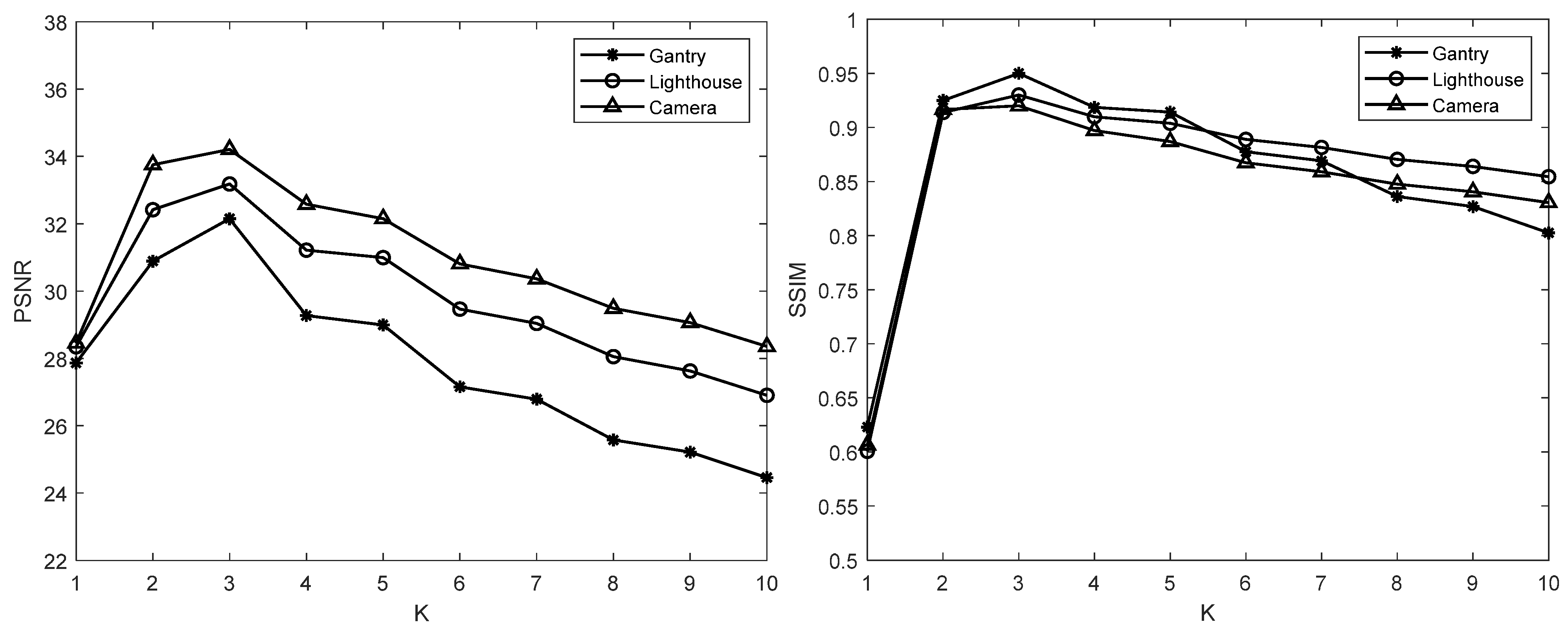
Since a slight increase in the group size will cause a large fluctuation in image denoising quality, tuning the value of the group size is very sensitive. Furthermore, an increase in the group size will increase the CPU time. To find the optimal group size K, a denoising experiment was carried out by varying the value of K, while all other parameters remained unchanged. Three images “Gantry”, “Lighthouse” and “Camera” with sizes of 260 × 260, 450 × 450 and 512 × 512 were used to obtain the best option of K. As observed from Figure 2, the best PSNR and SSIM values were obtained when $K=3$; hence, in the experiments, the group size was set to be 3.

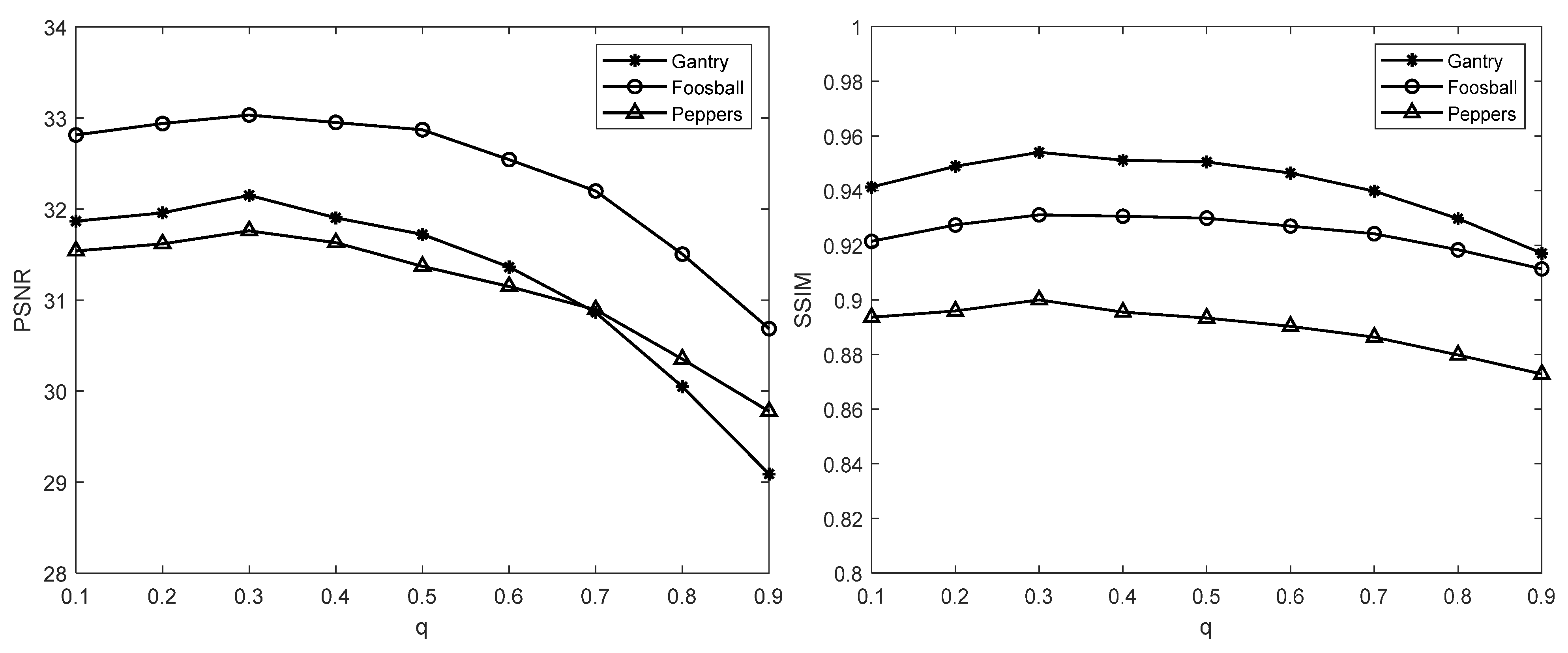
For restoring sharp and clear edges, the value of $q(0<q<1)$ in ℓ_q norm is important. By varying the value of q from 0.1 to 0.9 while holding all other parameters constant, then the denoising results for σ = 15 with different values of q for images “Peppers”, “Gantry” and “Foosball” are shown in Figure 3. As seen in the figure, the value of $q=0.3$ gives the best PSNR and SSIM in most cases. By this observation, $q=0.3$ is set in all subsequent experiments.

To test the influence of the fractional order on the value of PSNR, the proposed algorithm was applied to denoise images “Camera”, “Hallway”, “Parrot” and “Planes” with noise level σ = 15. The PSNR values of the denoised images processed by different values of the fractional order α in our model are listed in

Table 1. PSNR values with σ = 15 under different fractional order α.

α	Camera	Hallway	Parrot	Planes
1.0	33.9562	36.7828	33.3577	35.5842
1.1	34.1734	36.9008	33.4138	35.6634
1.2	34.2049	36.9644	33.5486	35.7519
1.3	34.1718	36.9445	33.4561	35.6872
1.4	34.1873	36.9039	33.4772	35.6516
1.5	34.1551	36.9161	33.4026	35.6633
1.6	34.1290	36.8760	33.3926	35.6024
1.7	34.1272	36.8339	33.3683	35.5833
1.8	34.0845	36.8497	33.3449	35.5661
1.9	34.0715	36.8308	33.3274	35.5621

For easy observation, the biggest PSNR values are shown in boldface.

. It is obvious that the parameter α has an effect on the result of denoising, and the best result often does not happen at α = 1, which means the proposed fractional order TV model outperforms the typical first-order TV model. The best value of the PSNR score is achieved when α = 1.2 from Table 1; as a result, this value of α = 1.2 is used in all of our experimental work.

4.2. Experiments on Image Denoising

The following experiments were conducted to validate the effectiveness of FQTV-OGS for denoising additive Gaussian noise. The proposed algorithm was compared visually and analytically with several state-of-the-art methods, namely FTV [27], OGSTV [37] and LLT [16]. In this simulation, zero-mean additive white Gaussian noise with standard variance σ = 15 and σ = 30 was added to 10 images, respectively, and the proposed algorithm was applied to process these given noisy images. The values of PSNR and SSIM of the restored images and computational time (in seconds) by four different methods are listed in

Table 2. Denoising results by different methods.

σ	Images	Proposed	FTV	OGSTV	LLT
		PSNR/SSIM/Time(s)	PSNR/SSIM/Time(s)	PSNR/SSIM/Time(s)	PSNR/SSIM/Time(s)
15	Lily	32.80/0.90/1.53	32.51/0.90/2.05	32.38/0.89/0.43	32.29/0.88/1.29
	Butterfly	31.80/0.94/3.29	31.51/0.92/2.42	31.27/0.90/0.63	31.05/0.90/1.27
	Foosball	33.01/0.93/3.07	32.77/0.92/2.27	32.52/0.92/0.67	31.87/0.90/1.10
	Peppers	32.34/0.92/0.79	32.12/0.91/1.10	31.99/0.91/0.18	31.54/0.91/0.41
	planes	35.72/0.92/1.14	35.40/0.92/1.41	35.11/0.91/0.21	34.33/0.90/0.52
	Gantry	32.15/0.95/0.94	31.98/0.94/1.50	31.51/0.93/0.30	30.70/0.90/0.63
	Lighthouse	33.18/0.93/3.93	32.92/0.91/2.86	32.85/0.91/0.85	32.15/0.90/1.52
	Parrot	33.55/0.91/1.14	33.18/0.90/1.69	32.81/0.90/0.57	32.66/0.89/0.55
	Camera	34.21/0.92/5.12	34.08/0.91/3.46	33.79/0.91/1.13	33.40/0.91/2.68
	Hallway	36.96/0.92/11.02	36.67/0.91/9.16	36.18/0.90/2.08	35.30/0.90/7.32
	(Average)	33.57/0.92/3.20	33.31/0.91/2.79	33.04/0.91/0.71	32.53/0.90/1.73
30	Lily	29.49/0.83/1.87	29.02/0.83/1.89	28.75/0.82/0.51	28.18/0.81/1.65
	Butterfly	28.07/0.89/3.65	27.51/0.88/3.20	27.29/0.87/0.95	26.72/0.86/2.07
	Foosball	29.31/0.89/3.47	28.89/0.88/2.70	28.35/0.87/1.37	27.49/0.83/0.94
	Peppers	28.78/0.87/0.93	28.52/0.86/1.22	28.22/0.85/0.21	27.75/0.85/0.57
	planes	32.49/0.90/1.20	32.05/0.89/1.61	31.68/0.88/0.60	30.82/0.86/1.12
	Gantry	28.14/0.89/1.43	28.15/0.89/1.48	27.48/0.86/0.43	26.58/0.81/0.87
	Lighthouse	29.77/0.89/4.61	29.46/0.88/3.55	29.04/0.85/1.31	28.35/0.84/2.55
	Parrot	30.27/0.87/1.75	29.81/0.87/1.66	29.42/0.86/0.64	29.08/0.84/0.79
	Camera	30.88/0.87/5.76	30.89/0.87/4.09	30.35/0.86/1.75	29.86/0.85/3.20
	Hallway	34.11/0.90/11.88	33.79/0.89/11.55	33.47/0.88/4.49	32.02/0.86/8.50
	(Average)	30.13/0.88/3.66	29.81/0.87/3.30	29.41/0.86/1.23	28.69/0.84/2.23

For easy observation, the biggest PSNR and SSIM values are shown in boldface.

.

As can be observed from Table 2, it is obvious that our method performed better in terms of PSNR and SSIM compared to the other three methods, with only a few exceptions, but the average PSNR and SSIM values of the images denoised by FQTV-OGS were still the highest. For the case of σ = 15, our method performed the best in terms of PSNR and SSIM values for all denoised images, based on Table 2. For experiments with σ = 30, the SSIM score of all test images denoised by our method was the best, and the FQTV-OGS method had better numerical results than all other methods in terms of PSNR for all images, except “Camera” and “Gantry”; the PSNR values of these two images denoised by the FTV approach with the noise level of σ = 30 were slightly higher than the results of our approach.

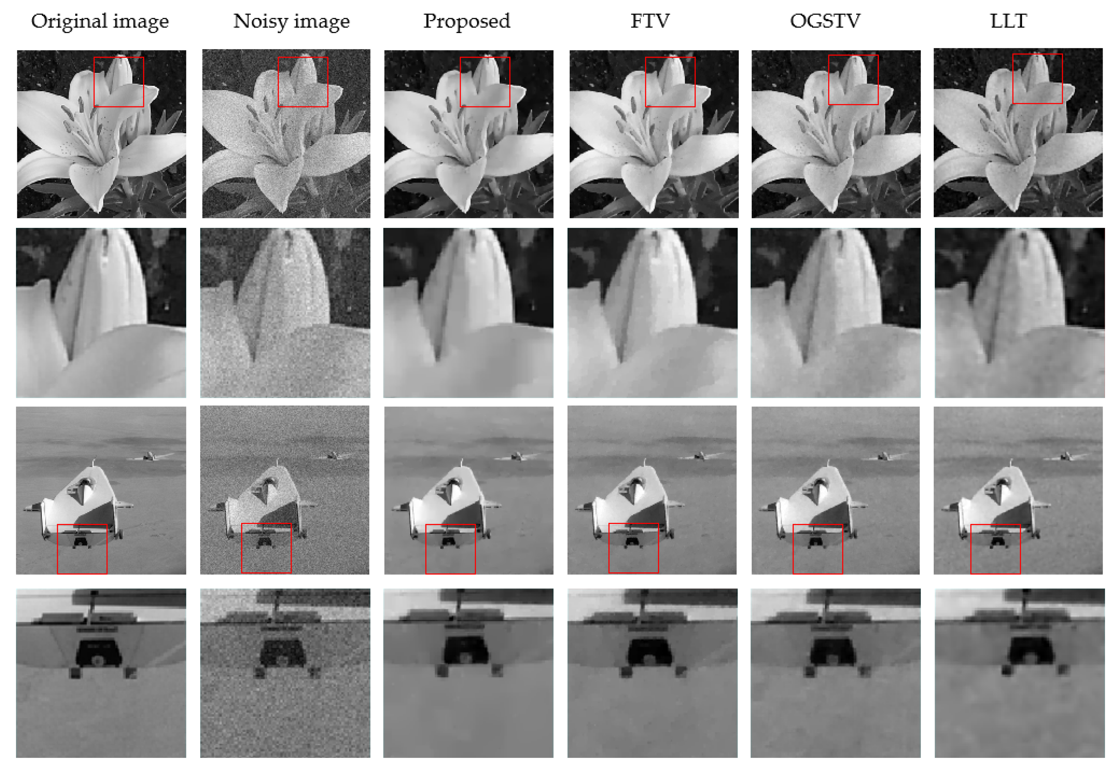
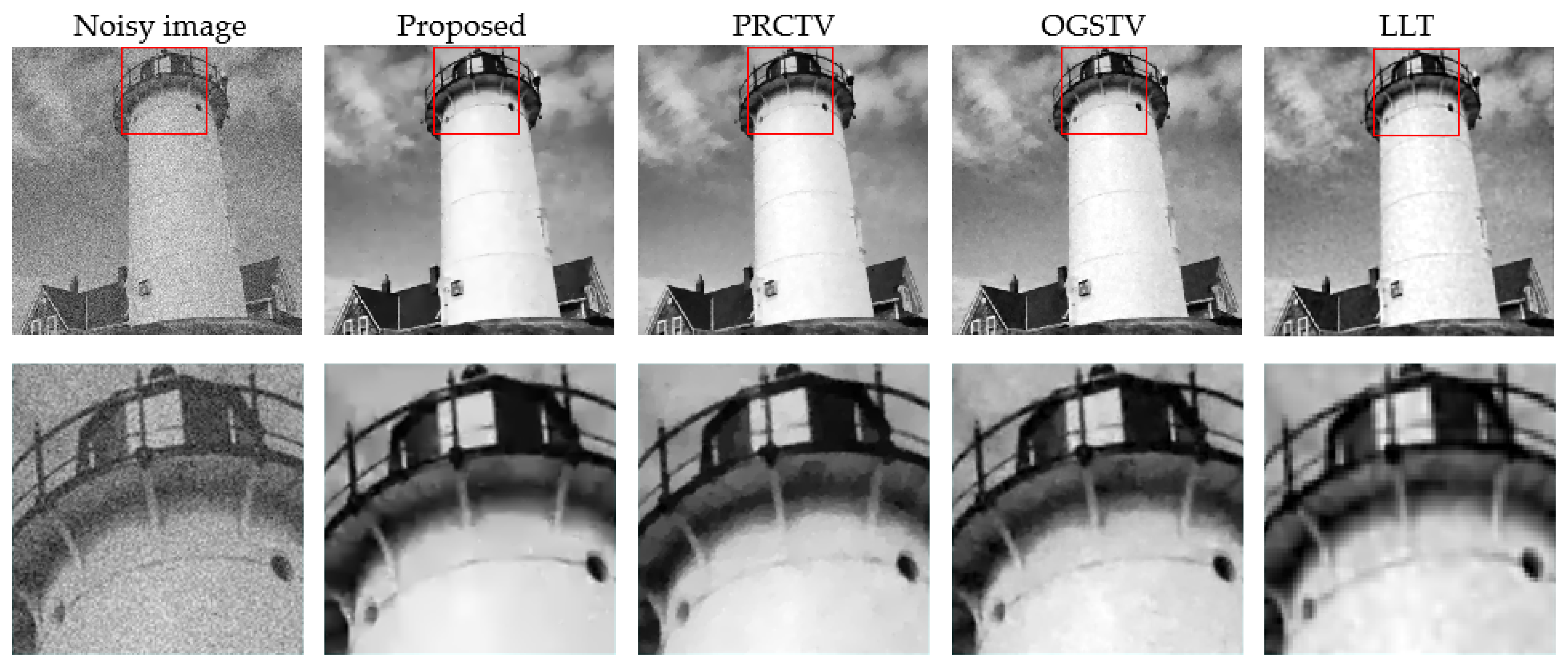
The denoising results of four different methods under noise level of σ = 15 and σ = 30 are illustrated in Figure 4 and Figure 5, respectively, where noisy images, the denoised images and the corresponding zoomed fragments are shown. From these figures, it is obvious that the denoised images obtained by the FTV method, OGSTV method and LLT always had different degrees of staircase artifacts and could not effectively preserve important texture features of images, while our method avoided this drawback effectively and performed the best visually.

4.3. Additional Comments on the Regularizers

In order to show the individual contribution of the regularizers on image denoising, the quality of the denoised images degraded by Gaussian noise with σ = 15 was considered. As already mentioned, the presented optimization framework makes use of two regularizers, “fractional order total variation with overlapping group sparsity” (FTV-OGS) and “ℓ_q norm based higher order total variation” (q-HTV).

Figure 6a,b show the noisy image “Camera” and the restored image using the FTV-OGS regularizer alone, respectively. As seen from Figure 6b, it is effective for noise removal, but the effect of restoring the edges of an image needs to be strengthened. By using the q-HTV regularizer only, the experimental results indicate that this regularizer owns a better ability to restore the edges of an image; however, the additive noise is not suppressed effectively which can be observed more clearly in the background of the image in Figure 6c. Combining both FTV-OGS regularizer and q-HTV regularizer in our optimization framework results in a better denoised image, retaining sharp edges and texture of the image, avoiding undesirable staircase artifacts, as shown in the Figure 6d.

4.4. Convergence

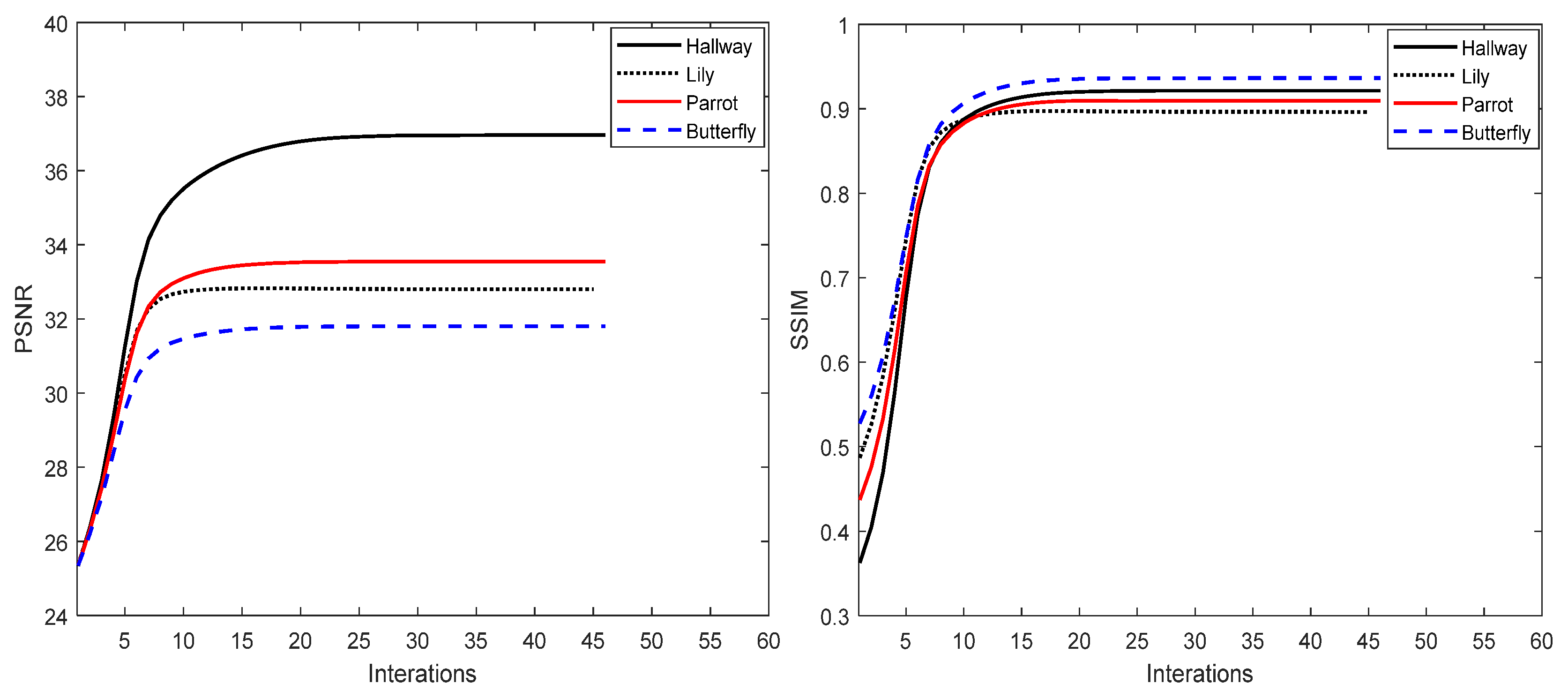
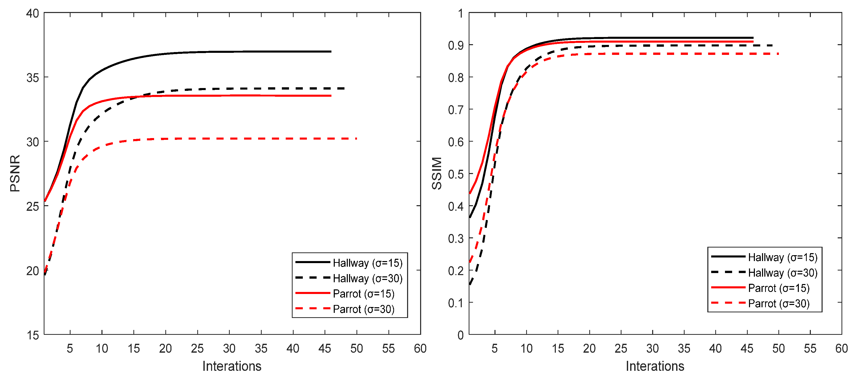
The convergence is an important factor for evaluating the performance of algorithm. Hence, the convergence of our algorithm was verified experimentally. For this purpose, the proposed algorithm is respectively used to process the images corrupted by the additive white Gaussian noise with noisy levels σ = 15 and σ = 30, and the PSNR value and the SSIM value are recorded at each iteration. From the Figure 7 and Figure 8, it is obvious that our proposed denoising algorithm is convergent.

5. Conclusions

On the basis of analyzing and summarizing previous research works, a new hybrid model for image denoising based on fractional order total variation with overlapping group sparsity and higher order total variation with ℓ_q norm, which was motivated by the fact that overlapping group sparsity could better exploit the sparsity characteristics of natural images to approximate the original images and that hybrid total variation model would mitigate the staircase artifacts more effectively.

By generalizing the alternating direction method of multipliers, a parallel linear ADMM framework was developed for tackling the proposed optimization model. The numerical experiments validated that our method outperformed other related three state-of-the-art methods in terms of PSNR and SSIM values for the outstanding performances of our approach in preserving details of images and avoiding the staircase artifacts. We plan to extend the proposed method to parameters adaptation and blind image restoration in future work.

References

1. Ribes, A.; Schmitt, F. Linear inverse problems in imaging. IEEE Signal Process. Mag. 2008, 25, 84–99. [Google Scholar] [CrossRef]
2. Gilton, D.; Ongie, G.; Willett, R. Neumann networks for linear inverse problems in imaging. IEEE Trans. Comput. Imaging 2019, 6, 328–343. [Google Scholar] [CrossRef]
3. Rudin, L.; Osher, S.; Fatemi, E. Nonlinear total variation based noise removal algorithms. Phys. D Nonlinear Phenom. 1992, 60, 259–268. [Google Scholar] [CrossRef]
4. Zhang, B.; Zhu, Z.; Xu, C. A primal-dual multiplier method for total variation image restoration. Appl. Numer. Math. 2019, 145, 145–158. [Google Scholar] [CrossRef]
5. Zhi, Z.; Shi, B.; Sun, Y. Primal-dual method to smoothing TV-based model for image denoising. J. Algorithms Comput. Technol. 2016, 10, 235–243. [Google Scholar] [CrossRef]
6. He, C.; Hu, C.; Li, X.; Zhang, W. A parallel primal-dual splitting method for image restoration. Inf. Sci. 2016, 358, 73–91. [Google Scholar] [CrossRef]
7. Cai, J.; Osher, S.; Shen, Z. Split Bregman methods and frame based image restoration. Multiscale Model. Simul. 2010, 8, 337–369. [Google Scholar] [CrossRef]
8. Kim, J.H.; Akram, F.; Choi, K.N. Image denoising feedback framework using split Bregman approach. Expert. Syst. Appl. 2017, 87, 252–266. [Google Scholar] [CrossRef]
9. Shi, B.; Pang, Z.F.; Yang, Y.F. A projection method based on the splitting Bregman iteration for the image denoising. J. Appl. Math. Comput. 2012, 39, 533. [Google Scholar] [CrossRef]
10. Chen, C.; Ng, M.K.; Zhao, X. Alternating direction method of multipliers for nonlinear image restoration problems. IEEE Trans. Image Process. 2014, 24, 33–43. [Google Scholar] [CrossRef]
11. Zhang, J.; Nagy, J.G. An effective alternating direction method of multipliers for color image restoration. Appl. Numer. Math. 2021, 164, 43–56. [Google Scholar] [CrossRef]
12. Sniba, F.; Karami, F.; Meskine, D. ADMM algorithm for some regularized Perona-Malik equation and applications to image denoising. Signal Image Video Process. 2023, 17, 609–617. [Google Scholar] [CrossRef]
13. Chan, T.; Marquina, A.; Mulet, P. High-order total variation-based image restoration. SIAM J. Sci. Comput. 2000, 22, 503–516. [Google Scholar] [CrossRef]
14. Lv, X.; Song, Y.; Wang, S.; Le, J. Image restoration with a high-order total variation minimization method. Appl. Math. Model. 2013, 37, 8210–8224. [Google Scholar] [CrossRef]
15. Thanh, D.N.; Prasath, V.S.; Hieu, L.M.; Dvoenko, S. An adaptive method for image restoration based on high-order total variation and inverse gradient. Signal Image Video Process. 2020, 14, 1189–1197. [Google Scholar] [CrossRef]
16. Lysaker, M.; Lundervold, A.; Tai, X. Noise removal using fourth-order partial differential equation with applications to medical magnetic resonance images in space and time. IEEE Trans. Image Process. 2003, 12, 1579–1590. [Google Scholar] [CrossRef]
17. Bredies, K.; Kunisch, K.; Pock, T. Total generalized variation. SIAM J. Imaging Sci. 2010, 3, 492–526. [Google Scholar] [CrossRef] [Green Version]
18. Gao, Y.; Liu, F.; Yang, X. Total generalized variation restoration with non-quadratic fidelity. Multidimens. Syst. Signal Process. 2018, 29, 1459–1484. [Google Scholar] [CrossRef]
19. Lv, Y. Total generalized variation denoising of speckled images using a primal-dual algorithm. J. Appl. Math. Comput. 2020, 62, 489–509. [Google Scholar] [CrossRef]
20. Liu, X.; Huang, L. A new nonlocal total variation regularization algorithm for image denoising. Math. Comput. Simul. 2014, 97, 224–233. [Google Scholar] [CrossRef]
21. Li, Z.; Malgouyres, F.; Zeng, T. Regularized non-local total variation and application in image restoration. J. Math. Imaging Vis. 2017, 59, 296–317. [Google Scholar] [CrossRef] [Green Version]
22. Jidesh, P.; Holla, S. Non-local total variation regularization models for image restoration. Comput. Electr. Eng. 2018, 67, 114–133. [Google Scholar] [CrossRef]
23. Dong, F.; Chen, Y. A fractional-order derivative based variational framework for image denoising. Inverse Probl. Imaging. 2016, 10, 27–50. [Google Scholar] [CrossRef] [Green Version]
24. Li, X.; Meng, X.; Xiong, B. A fractional variational image denoising model with two-component regularization terms. Appl. Math. Comput. 2022, 427, 127178. [Google Scholar] [CrossRef]
25. Chen, D.; Chen, Y.; Xue, D. Fractional-order total variation image denoising based on proximity algorithm. Appl. Math. Comput. 2015, 257, 537–545. [Google Scholar] [CrossRef]
26. Tian, D.; Xue, D.; Wang, D. A fractional-order adaptive regularization primal-dual algorithm for image denoising. Inf. Sci. 2015, 296, 147–159. [Google Scholar] [CrossRef]
27. Mei, J.J.; Dong, Y.; Huang, T.Z. Simultaneous image fusion and denoising by using fractional-order gradient information. J. Comput. Appl. Math. 2019, 351, 212–227. [Google Scholar] [CrossRef]
28. Liu, J.; Ma, R.; Zeng, X.; Liu, W.; Wang, M.; Chen, H. An efficient non-convex total variation approach for image deblurring and denoising. Appl. Math. Comput. 2021, 397, 125977. [Google Scholar] [CrossRef]
29. Zha, Z.; Zhang, X.; Wu, Y.; Wang, Q.; Liu, X.; Tang, L.; Yuan, X. Non-convex weighted p nuclear norm based ADMM framework for image restoration. Neurocomputing 2018, 311, 209–224. [Google Scholar] [CrossRef]
30. Guo, J.; Chen, Q. Image denoising based on nonconvex anisotropic total-variation regularization. Signal Process. 2021, 186, 108124. [Google Scholar] [CrossRef]
31. Yang, J.; Zhao, X.; Mei, J.; Wang, S.; Ma, T.; Huang, T. Total variation and high-order total variation adaptive model for restoring blurred images with Cauchy noise. Comput. Math. Appl. 2019, 77, 1255–1272. [Google Scholar] [CrossRef]
32. Kazemi Golbaghi, F.; Rezghi, M.; Eslahchi, M.R. A hybrid image denoising method based on integer and fractional-order total variation. Iran. J. Sci. Technol. Trans. A-Sci. 2020, 44, 1803–1814. [Google Scholar] [CrossRef]
33. Adam, T.; Paramesran, R. Image denoising using combined higher order non-convex total variation with overlapping group sparsity. Multidimens. Syst. Signal Process. 2019, 30, 503–527. [Google Scholar] [CrossRef]
34. Tang, L.; Ren, Y.; Fang, Z.; He, C. A generalized hybrid nonconvex variational regularization model for staircase reduction in image restoration. Neurocomputing 2019, 359, 15–31. [Google Scholar] [CrossRef]
35. Peyré, G.; Fadili, J. Group sparsity with overlapping partition functions. In Proceedings of the 2011 19th European Signal Processing Conference, Barcelona, Spain, 29 August–2 September 2011; IEEE: Manhattan, NY, USA, 2011; pp. 303–307. [Google Scholar]
36. Selesnick, I.W.; Chen, P. Total variation denoising with overlapping group sparsity. In Proceedings of the 2013 IEEE International Conference on Acoustics, Speech and Signal Processing, Vancouver, BC, Canada, 26–31 May 2013; pp. 5696–5700. [Google Scholar]
37. Liu, J.; Huang, T.; Selesnick, I.W.; Lv, X.; Chen, P. Image restoration using total variation with overlapping group sparsity. Inf. Sci. 2015, 295, 232–246. [Google Scholar] [CrossRef] [Green Version]
38. Zhu, J.; Wei, Y.; Wei, J.; Hao, B. A Non-Convex Hybrid Overlapping Group Sparsity Model with Hyper-Laplacian Prior for Multiplicative Noise. Fractal Fract. 2023, 7, 336. [Google Scholar] [CrossRef]
39. Kumar, A.; Ahmad, M.O.; Swamy, M.N.S. An efficient denoising framework using weighted overlapping group sparsity. Inf. Sci. 2018, 454, 292–311. [Google Scholar] [CrossRef]
40. Jon, K.; Sun, Y.; Li, Q.; Liu, J.; Wang, X.; Zhu, W. Image restoration using overlapping group sparsity on hyper-Laplacian prior of image gradient. Neurocomputing 2021, 420, 57–69. [Google Scholar] [CrossRef]
41. Ding, M.; Huang, T.; Wang, S.; Mei, J.; Zhao, X. Total variation with overlapping group sparsity for deblurring images under Cauchy noise. Appl. Math. Comput. 2019, 341, 128–147. [Google Scholar] [CrossRef]
42. Yin, M.; Adam, T.; Paramesran, R.; Hassan, M.F. An 0-overlapping group sparse total variation for impulse noise image restoration. Signal Process.-Image Commun. 2022, 102, 116620. [Google Scholar] [CrossRef]
43. Micchelli, C.A.; Shen, L.; Xu, Y. Proximity algorithms for image models: Denoising. Inverse Probl. 2011, 27, 045009. [Google Scholar] [CrossRef]
Figure 1. Images for the numerical experiments. (a) Peppers (256 × 256); (b) Gantry (260 × 260); (c) Parrot (300 × 300); (d) Planes (300 × 300); (e) Lily (350 × 350); (f) Foosball (400 × 400); (g) Butterfly (400 × 400); (h) Lighthouse (450 × 450); (i) Camera (512 × 512); (j) Hallway (800 × 800).
Fractalfract 07 00573 g001aFractalfract 07 00573 g001b
Figure 2. PSNR and SSIM values for images denoised by FQTV-OGS with different group sizes (Noise standard variance σ = 15).
Fractalfract 07 00573 g002
Figure 3. PSNR and SSIM values with different q.
Fractalfract 07 00573 g003
Figure 4. Denoised images of different approaches and the corresponding zoomed fragments under noise level of σ = 15.
Fractalfract 07 00573 g004
Figure 5. Comparison of different methods for the image ‘‘Lighthouse’’ with σ = 30.
Fractalfract 07 00573 g005
Figure 6. (a) Noisy image under noise level of σ = 15; The restored images obtained by (b) only FTV-OGS as the regularizer; (c) only q-HTV as the regularizer; (d) using both regularizers (proposed method).
Fractalfract 07 00573 g006
Figure 7. The convergence of the proposed method under noise level of σ = 15 with the iteration number for different images.
Fractalfract 07 00573 g007
Figure 8. The convergence of the proposed method with the iteration numbers under different noise levels for “Hallway” and “Parrot”.
Fractalfract 07 00573 g008