Dynamic Analysis and Control of a Financial System with Chaotic Behavior Including Fractional Order

Abstract

This paper presents the results of investigating the dynamics of an economic system with chaotic behavior and a suboptimal control proposal to suppress the chaotic behavior. Numerical results using phase portraits, bifurcation diagrams, Lyapunov exponents, and 0-1 testing confirmed chaotic and hyperchaotic behavior. The results also proved the effectiveness of the control, showing errors below 1%, even in cases where the control design is subject to parametric errors. Additionally, an investigation of the system in fractional order is included, demonstrating that the system has periodic, constant, or chaotic behavior for specific values of the order of the derivative.

1. Introduction

In recent years, modeling financial and economic systems with chaotic behavior as non-linear systems has aroused the interest of researchers in various fields of knowledge [1]. Financial systems are intricate non-linear systems that interact with the environment and contain many complex factors, making it practically impossible to make convincing economic predictions for financial systems with chaotic behavior, justifying the relevance of studying their dynamics and control projects [2,3,4,5,6,7].

Following this trend, the number of investigations seeking to explain the influence of structural variations, uncertainties in microeconomic and macroeconomic variations, irregular increases, and effects of parameters on the dynamics of financial and economic systems has grown, as well as the emergence of chaotic behavior [8,9]. The non-linearities and chaotic behavior of stock markets have been investigated by [10,11]. The authors concluded that the analyzed action systems have a chaotic behavior and that their non-linearities must be considered. In this sense, the dynamic analysis of an economic system with this type of behavior is presented in [5]. Phase diagrams, bifurcation diagrams, and time histories are presented to prove the chaotic behavior. In [6] is given the dynamic model of an economic and financial system oscillator based on the theory of automatic control systems. Computational results indicate that the proposed model makes generating chaotic economic variations and their synchronization in a set of coupled economic variations possible.

Studies demonstrate that the behavior of economic and financial systems in the present can be affected by the history of variables such as exchange rates, gross domestic product, interest rates, production, and stock prices. This memory effect can last for long periods, meaning that past behaviors can interfere with economic systems’ current and future behavior, thus correlating past economic disturbances with future economic variations [12]. According to [12], the fact that economic variables have long memories makes fractional calculus adequate to study the dynamic behavior of economic systems. Thus, the number of investigations of applying a fractional order in financial and economic systems dynamics has grown [1]. In [13], a dynamic analysis of a financial system in fractional order using phase diagrams and Lyapunov exponents was presented. In [1], a financial system in fractional order was considered. Computational results demonstrated that the system exhibits chaotic behavior for specific parameters in integer or fractional order analysis. The chaotic behavior was determined by analyzing bifurcation diagrams, Lyapunov exponents, and the Kaplan–Yorke dimension. In [14], an active control technique controlled chaotic behavior in a fractional-order economic system. Computational results demonstrated that the proposed control is efficient in suppressing chaos. The application of adaptive control to stop the chaotic behavior of a financial system was considered in [15]. In [7], the dynamic analysis of an economic system with chaotic behavior was performed through bifurcation diagrams and Lyapunov exponent calculation. To eliminate chaotic behavior, the introduction of an adaptive control system was considered. Numerical simulations demonstrated that the proposed control is efficient in suppressing chaos and can be applied for synchronization and anti-synchronization of the system.

Delayed feedback control systems have been considered to suppress chaotic behavior in fractional order systems [16,17,18,19] and for use in a financial system with chaotic behavior in [4]. Computational results showed that the fractional order influences the system’s stability and Hopf bifurcation. In [20], the dynamic analysis of an economic system with chaotic behavior is presented, using an adaptive control by sliding modes in the chaos control. The 0-1 test and the Lyapunov exponent prove the chaotic behavior. In [21], the 0-1 test and the Lyapunov exponent were used to identify chaotic behavior in an economic system represented by fractional order. In addition to the dynamic analysis, the authors propose a synchronization system. Impulsive control is considered in [22] in controlling the chaotic behavior of a financial system with delayed feedback with a Markovian jump, with partially unknown variations in quotations. The dynamic analysis of a financial system with four degrees of freedom in fractional order and with the inclusion of a financial incentive using the 0-1 test is considered in [23]. In [24], the 0-1 test was used to determine the chaotic behavior of the trust effect in a financial system in fractional order. A financial system in fractional order is investigated in [25]. Numerical results showed a hyperchaotic behavior of the system. Hyperchaos was also detected by [26] in a financial system in fractional order. The authors proposed a sliding mode control with a neural network estimator to control and synchronize the financial system in fractional order. Synchronization of a financial system in fractional order is also investigated in [27].

Motivated by the previous works, we present an extensive investigation of the financial system proposed by [5] and considered in [7], evaluating the system in integer and fractional order. The present work contributes to the body of knowledge by studying the influence of the six main parameters of the mathematical model through diagrams, bifurcation diagrams, and the Lyapunov exponent in case the system is in integer order. To determine the chaotic behavior in the system in fractional order, the 0-1 test, initially proposed by [28], was performed and successfully used to analyze the chaotic behavior of systems in fractional order in [29,30,31,32]. To suppress the chaotic behavior of the system, a feedforward control and a feedback control obtained with the SDRE control were used. SDRE control was first proposed by [33] and successfully used to suppress chaotic behavior in [34].

Thus, this work aims to present the dynamic analysis of six of the eight parameters of the system, having performed this dynamic analysis of the system in fractional order through the use of the 0-1 test. The work also proposed using the SDRE control (State-Dependent Riccati Equation) to suppress chaos in economic and financial systems, whose robustness was demonstrated for parametric and fractional order variations.

The sections are presented as follows: The mathematical model and the dynamic analysis of the system for variations of six parameters is presented in Section 2. This section shows the variation of the first two Lyapunov exponents, demonstrating the existence of chaos and hyperchaos. Time histories and phase diagrams are presented for the parameters that generate the largest Lyapunov exponents. The bifurcation diagram is also shown to determine the chaotic behavior and the maximum peaks of each considered state variable. The 0-1 method and the analysis of the system’s behavior for variations in fractional order are also presented. Section 3 describes the proposed control, considering integer order and fractional order. This section also demonstrates the robustness of the control for parametric variations and its effectiveness in controlling the system in fractional order. Finally, Section 4 presents the conclusions and final considerations.

2. Dynamic Analysis

In this section, the dynamic analysis of a financial system is presented, represented by a mathematical model with three degrees of freedom; it was also recently considered in [5,7].

2.1. Mathematical Model

Equation (1) represents the economic and financial model proposed by [5] and investigated in this paper.

$$\begin{array}{l}{\dot{x}}_1=f{x}_3+x_2{x}_1-a{x}_1\\ {\dot{x}}_2=-b{x}_2^2-h{x}_1^2+e\\ {\dot{x}}_3=-c{x}_3-g{x}_1-d{x}_2\end{array}$$

(1)

where the state ($x_1$) represents the interest rate, the state ($x_2$) represents the investment demand, and the state ($x_3$) the price index. The parameters a, b, c, d, e, f, and g are constants.

According to [5,7], it can be observed that the interest rate variation ($x_1$) is proportional to the price index ($x_3$), and that investment demand ($x_2$) influences the interest rate. If the investment demand exceeds the value of savings, the financial institution will increase the interest rate. If the investment demand is low, the value of savings may exceed the investment demand, leading to the need to reduce the interest rate to encourage loaning.

Regarding the parameters of Equation (1), (e) represents the natural growth rate of investment demand ($x_2$). If the interest rate increases, the investment will be negatively affected, showing that excessive need for investment ($x_2$) will lead to a decrease in the rate of change in investment demand, represented by the term $-b{x}_2^2$, i.e., the rate of change in investment demand is negatively correlated with the square of the investment demand.

According to [5,7], the interest rate is negatively correlated with the price index variation rate given by (g). The price index variation rate decreases with the investment demand increase. It implies that increased investment demand leads to increased production, resulting in a price decrease. On the other hand, the decline in investment demand ($x_2$) causes a reduction in the number of products on the market, leading to an increase in the product’s price.

The following sections present the dynamic analysis of the system (1), initially considering the parameters: a = 0.3, b = 0.02, c = 1, d = 0.05, e = 1, f = 1.2, g = 1, and h = 0.1, with initial conditions x₁(0) = 0.2, x₂(0) = 0.5, and x₃(0) = 0.6. The Matlab^R ODE45 integrator was used for numerical simulations, with integration step (0.01). The Jacobian algorithms [35] were considered for calculating the Lyapunov exponent, with a simulation time of t = 2000. Codes available at Supplementary Materials S1.

2.2. Dynamic Analysis for Parametric Variations

To analyze the dynamic behavior of the system (1), initially, the parameters that represent the value of savings (a), the cost per investment (b), and the elasticity of demand in commercial markets (c) were varied.

Figure 1 shows the maximum values of the first two Lyapunov exponents, considering parameter variations: $a=[0:1]$, $b=[0:0.1]$, and $c=[0.1:3]$.

Analyzing the results presented in Figure 1, we can observe that system (1) has chaotic behavior for values of (c) close to 1 (Figure 1c,e) and that (c) is the most influential parameter for the chaotic behavior of the system. For the parameters $a=0.3$, $b=0.01$, and $c=0.3$, we have ${\lambda }_1=0.21$ (the first most prominent Lyapunov exponent) and ${\lambda }_2=0.0002$ (the second most prominent Lyapunov exponent). And according to [31], two positive Lyapunov exponents indicate hyperchaotic behavior.

Then, we considered the dynamic analysis of the system (1) for variations in parameter (e), which represents the natural growth rate of investment demand ($x_2$), parameter (f), which corresponds to the coefficient of variation of the interest rate ($x_1$) depending on the price index ($x_3$), and parameter (g), which represents the price index reduction coefficient ($x_3$) related to the interest rate variation ($x_1$).

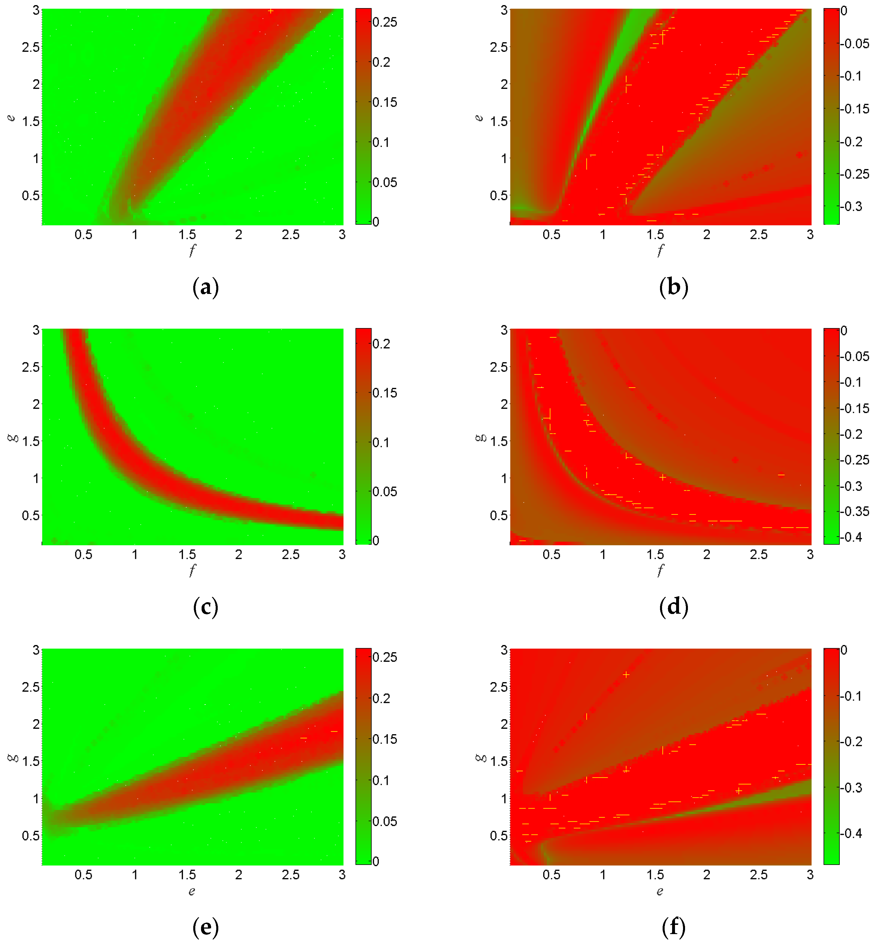
Figure 2 shows the maximum values of the first two Lyapunov exponents, considering $a=0.3$, $b=0.01$, and $c=0.3$, and variations in the parameters $f=[0.1:3]$, $e=[0.1:3]$, and $g=[0.1:3]$.

Considering the new results for the largest Lyapunov exponent presented in Figure 2, it can be observed in the color bars that the variation of parameters (e), (f), and (g) generated higher values of the first Lyapunov exponent. For a = 0.3, b = 0.01, c = 1, d = 0.05, e = 2.58, f = 2.1, g = 1, and h = 0.1, we have ${\lambda }_1=0.2635$ (first largest Lyapunov exponent) and ${\lambda }_2=0.0002$ (second largest Lyapunov exponent), values that indicate hyperchaotic behavior [36].

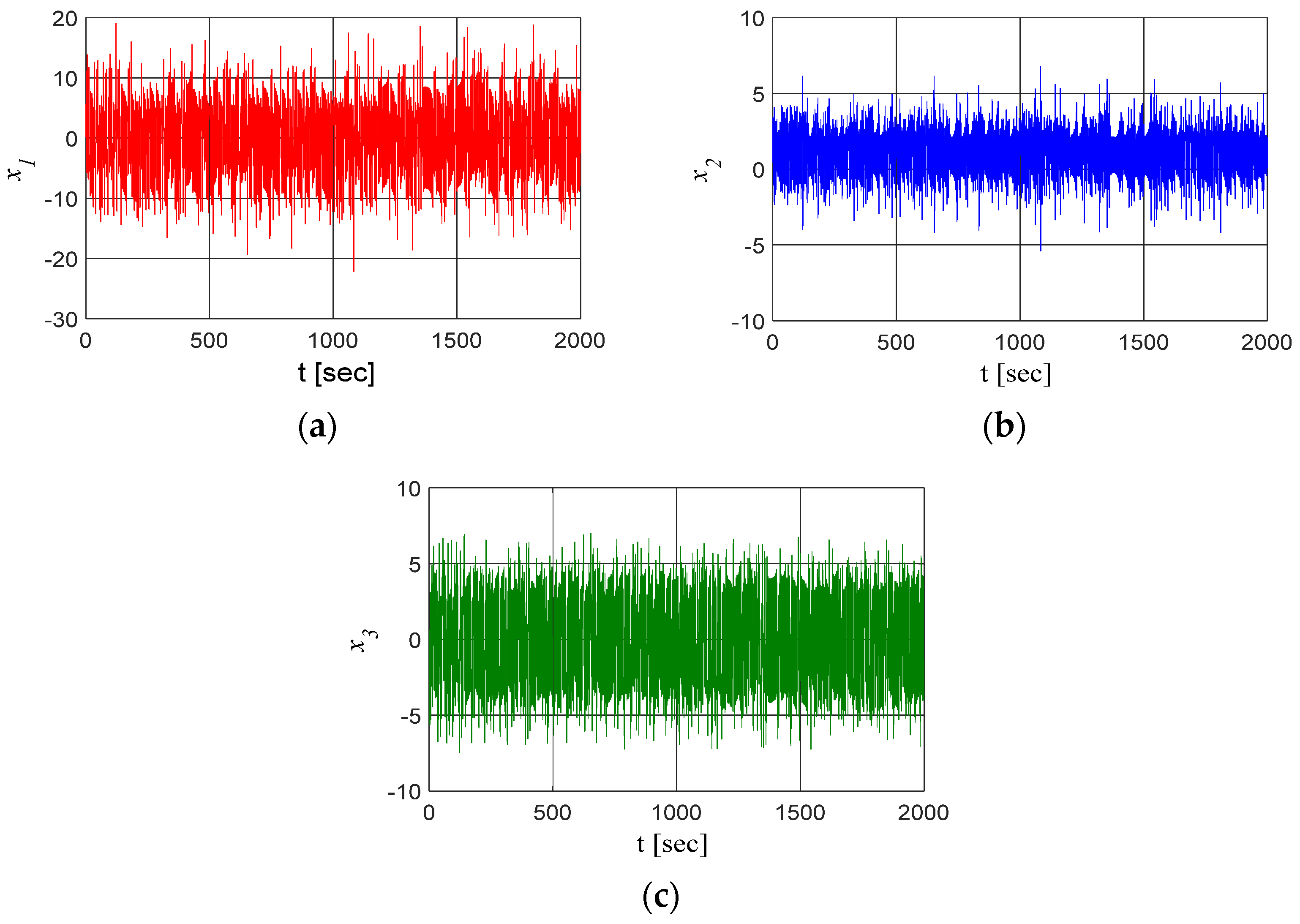
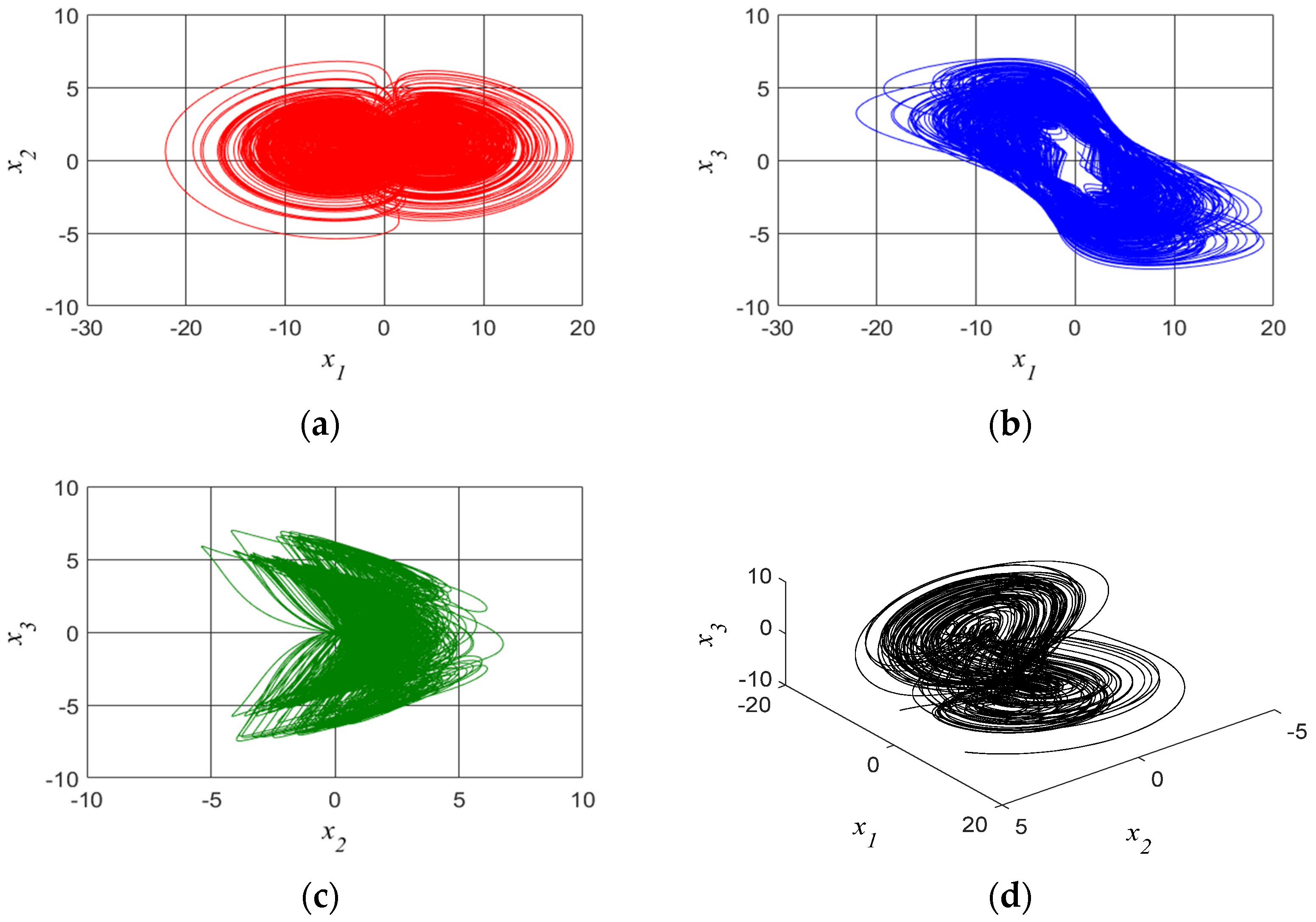
Figure 3 shows the time histories, and Figure 4 shows the phase diagrams for parameters a = 0.3, b = 0.01, c = 1, d = 0.05, e = 2.58, f = 2.1, g = 1, and h = 0.1. These values will be used in the rest of the paper.

As can be seen in Figure 3 and Figure 4, the system has a chaotic behavior and, according to the second largest Lyapunov exponent (${\lambda }_2=0.0002$), the system also has a hyperchaotic behavior, which are undesirable behaviors for an economic system since its unpredictability makes planning for future investments difficult.

In Figure 5, we present the bifurcation diagrams for the state peaks ($x_1$), considering the parameters (a, b, c, e, f, and g) investigated in this work. The state ($x_1$) was considered in the analysis, as it is the state that represents the interest rate and thus represents an essential role in the investment process [7,15,37].

As seen in Figure 5, parameters (a) and (b) did not significantly influence the chaotic behavior of the system. However, the influence of other parameters is evident; it is possible to eliminate the chaotic behavior by considering variations in the parameters (c, e, f, and g).

We can see in Figure 5e that parameter (e), which represents the natural growth rate of investment demand x₂, plays a vital role in controlling chaotic behavior, as well as in the maximum values of interest rates. It is possible to obtain a periodic behavior with rates below 5 units for $e=[0.1:1.654]\cup [1.74:1.852]$ or $f=[2.635:3]$, and periodic behavior with period 1 for the following cases: $c=[0.1:0.48]\cup [1.62:3]$, or $e=[0.1:1.654]$, or $f=[0.1:1.28]\cup [2.635:3]$, or $g=[0.1:0.66]\cup [1.38:3]$.

2.3. Dynamic Analysis for Fractional Order

This section presents the dynamic analysis of the economic system in fractional order. We considered the Riemann–Liouville operator [34,38,39]. The operator was considered because it is already well known and has been used efficiently in different types of systems, as it does not require the system to be continuous at the origin or to be differentiable [34].

The Riemann–Liouville operator is given by [38]:

$$D^{q}x(t)=\frac{1}{\mathsf{\Gamma }\left(\eta -q\right)}{\displaystyle \underset{t_0}{\overset{t}{\int }}\frac{x^{(\eta )}(z)}{{\left(t-z\right)}^{q-\eta +1}}}dz$$

(2)

In case that $q=1$, one has the usual derivative. In this paper, $0<q\le 1$ will be considered, as it is the interval normally used in economic and financial systems and is particularly relevant for the study of dynamics in fractional order.

Equation (3) represents the economic system (1) in fractional order:

$$\begin{array}{l}\frac{d^{q_1}{x}_1}{d{t}^{q_1}}=f{x}_3+x_2{x}_1-a{x}_1\\ \frac{d^{q_2}{x}_2}{d{t}^{q_2}}=-b{x}_2^2-h{x}_1^2+e\\ \frac{d^{q_3}{x}_3}{d{t}^{q_3}}=-c{x}_3-g{x}_1-d{x}_2\end{array}$$

(3)

We considered $q_1=q_2=q_3=q$ and $0<q\le 1$. For numerical simulations, we considered the algorithm proposed by [38].

Application of 0-1 Test

The 0-1 test is an efficient method for quantitatively determining the chaotic behavior of a database [40,41,42]. It was proposed by [28,40], and successfully used in systems from different areas of knowledge, including economic and financial systems represented in fractional order [20,21,23,24]. The method consists in determining a parameter, $K=[0:1]$. The data are considered chaotic for values of K close to 1, whereas for values of K close to zero, a periodic behavior is considered [29,30,31,32]. The 0-1 test is considered in this section; for analysis, the variable $x_1$ behavior was chosen, considering the systems (3).

The test considers two new coordinates, $\left(p,q\right)$, and a system variable, $z_i$. The coordinates $\left(p,q\right)$ were obtained by [41,42]:

$$p={\displaystyle \sum _{i=0}^{n}z(i)}\cos (i\overline{\sigma })$$

(4)

$$q={\displaystyle \sum _{i=0}^{n}z(i)}\sin (i\overline{\sigma })$$

(5)

The parameter $\overline{\sigma }\in (0,\pi )$ is a constant. The mean square displacement of the new variables $p$ and $q$ was given by [41,42]:

$$M(n,\sigma )=\underset{n\to \infty }{\lim }\frac{1}{N}{\displaystyle \sum _{i=1}^N\left[{\left(p(i+n,\overline{\sigma })-p(i,\overline{\sigma })\right)}^2+{\left(q(i+n,\overline{\sigma })-q(i,\overline{\sigma })\right)}^2\right]}$$

(6)

where $n=1,2,\dots ,N$ and, therefore, we obtained the parameter $K_c$ within the limit of a very long time [41,42]:

$$K_c=\frac{\mathrm{cov}\left(Y,M\left(\overline{\sigma }\right)\right)}{\sqrt{\mathrm{var}\left(Y\right)\mathrm{var}\left(M\left(\overline{\sigma }\right)\right)}}$$

(7)

where $M(\overline{\sigma })=\left[M(1,\overline{\sigma }),M(2,\overline{\sigma }),\dots ,M(n_{\max },\overline{\sigma })\right]$ and $Y=\left[1,2,\dots ,n_{\max }\right]$.

Given any two vectors $z$ and $y$, the covariance $\mathrm{cov}(z,y)$ and variance $\mathrm{var}(z)$ of $n_{\max }$ elements are usually defined as [25]:

$$\mathrm{cov}(z,y)=\frac{1}{n_{\max }}{\displaystyle \sum _{n=1}^{n_{\max }}\left(z(n)-\overline{z}\right)}\left(y(n)-\overline{y}\right)$$

(8)

$$\mathrm{var}(z)=\mathrm{cov}(z,y)$$

(9)

where $\overline{z}$ is the average of $z(n)$ and $\overline{y}$ is the average of $y(n)$.

In this paper, $n={10}^4$ and $i=\frac{n}{{10}^2},\dots ,\frac{n}{10}$.

Figure 6 presents the state $x_1$ for variations in the order of the fractional derivative; $q_1=q_2=q_3=q=\left[0.7:1\right]$ was considered in the simulations.

Applying the 0-1 test to the data in Figure 6, we obtain: $K=0$ for $q=0.7$, $K=0$ for $q=0.75$, $K=0.99$ for $q=0.80$, $K=0$ for $q=0.85$, $K=0$ for $q=0.9$, $K=0$ for $q=0.95$, and $K=0.99$ for $q=1$.

It is possible see in Figure 6 results indicating that the order of the fractional derivative influences the dynamics of the system, which can be oscillatory and periodic ($q=0.85$, $q=0.9$, and $q=0.95$), can stabilize at a fixed point ($q=0.7$ and $q=0.75$), or can be chaotic, as observed for the case of $q=0.80$. The results presented demonstrate the influence of memory on the dynamics of the economic model (Equation (1)), confirming that past behaviors and results can influence present results and that the use of fractional order can be used to represent economic variables with memory.

3. Proposed Control by SDRE Control and Feedforward Control

The SDRE control was utilized to avoid the system’s chaotic behavior. The objective was to establish a control so that the response of the controlled system (1) resulted in a desired state $x_i^{*}(t)$ that was asymptotically stable.

3.1. Integer Order System

Equation (10) represents the system (1), with the introduction of control signal $U$:

$$\begin{array}{l}{\dot{x}}_1=f{x}_3+x_2{x}_1-a{x}_1+U_1\\ {\dot{x}}_2=-b{x}_2^2-h{x}_1^2+e+U_2\\ {\dot{x}}_3=-c{x}_3-g{x}_1-d{x}_2+U_3\end{array}$$

(10)

where: $U=u+u^{*}$, $u$ is the state feedback control, and $u^{*}$ is the feedforward control.

The feedforward control is responsible for maintaining the system in a desired trajectory and is given by:

$$\begin{array}{l}{u}_1^{*}=-f{x}_3^{*}-x_2^{*}{x}_1^{*}+a{x}_1^{*}+{\dot{x}}_1^{*}\\ u_2^{*}=b{x}^{*}{}_2^2+h{x}^{*}{}_1^2-e+{\dot{x}}_2^{*}\\ u_3^{*}=c{x}_3^{*}+g{x}_1^{*}+d{x}_2^{*}+{\dot{x}}_3^{*}\end{array}$$

(11)

where: $x_1^{*}$, $x_2^{*}$, and $x_3^{*}$ are the desired states.

We substituted (11) in (10) and considered defining the errors:

$$\left[\begin{array}{c}{e}_1\\ e_2\\ e_3\end{array}\right]=\left[\begin{array}{c}{x}_1-x_1^{*}\\ x_2-x_2^{*}\\ x_3-x_3^{*}\end{array}\right]$$

(12)

The following system was obtained with regard to errors:

$$\begin{array}{l}{\dot{e}}_1=-a{e}_1+f{e}_3+e_1{e}_2+e_2{x}_1^{*}+e_1{x}_2^{*}+u_1\\ {\dot{e}}_2=-b{e}_2^2-2b{e}_2{x}_2^{*}-h{e}_1^2-2h{e}_1{x}_1^{*}+u_2\\ {\dot{e}}_3=-c{e}_3-g{e}_1-d{e}_2+u_3\end{array}$$

(13)

The system (13) can be represented in matrix form:

$$\left[\begin{array}{c}{\dot{e}}_1\\ {\dot{e}}_2\\ {\dot{e}}_3\end{array}\right]=\left[\begin{array}{ccc}-a+x_2^{*}& e_1+x_1^{*}& f\\ -h{e}_1-2h{x}_1^{*}& -b{e}_2-2b_2^{*}& 0\\ -g& -d& -c\end{array}\right]\hspace{0.17em}\left[\begin{array}{c}{e}_1\\ e_2\\ e_3\end{array}\right]+\left[\begin{array}{ccc}1& 0& 0\\ 0& 1& 0\\ 0& 0& 1\end{array}\right]\hspace{0.17em}\left[\begin{array}{c}{u}_{r_1}\\ u_{r_2}\\ u_{r_3}\end{array}\right]$$

(14)

Control $u$ is obtained from the following equation [34]:

$$u=-R^{-1}{B}^{T}P\hspace{0.17em}e=-Ke$$

(15)

where P is a symmetric matrix, and is obtained from the algebraic Riccati equation:

$$PA+A^{T}P-PB{R}^{-1}{B}^{T}P+Q=0$$

(16)

According to [33], the control $u$ is suboptimal, minimizing the function:

$$J={\displaystyle \underset{0}{\overset{\infty }{\int }}(}{e}^{T}Qe+u^{T}R\hspace{0.17em}u)dt$$

(17)

The matrices $A$ and $B$ of the system (15) are represented by:

$$A=\left[\begin{array}{ccc}-a+x_2^{*}& e_1+x_1^{*}& f\\ -h{e}_1-2h{x}_1^{*}& -b{e}_2-2b{x}_2^{*}& 0\\ -g& -d& -c\end{array}\right]\mathrm{and}B=\left[\begin{array}{ccc}1& 0& 0\\ 0& 1& 0\\ 0& 0& 1\end{array}\right]$$

(18)

We defined Q and R matrices:

$$Q={10}^3\left[\begin{array}{ccc}1& 0& 0\\ 0& 1& 0\\ 0& 0& 1\end{array}\right]$$

(19)

First of all, it is crucial to define the desired states: $x_1^{*}$, $x_2^{*}$, and $x_3^{*}$. Analyzing the results of Figure 6a,b, we can see that $x_1^{*}\approx 5$ when we consider the system memory. To keep the interest rate close to this value, we define $x_1^{*}=5$ as desired in this paper. Setting up $x_1^{*}=5$ as an equilibrium point, we obtain: $x_2^{*}=2.8284$ and $x_3^{*}=4.8586$.

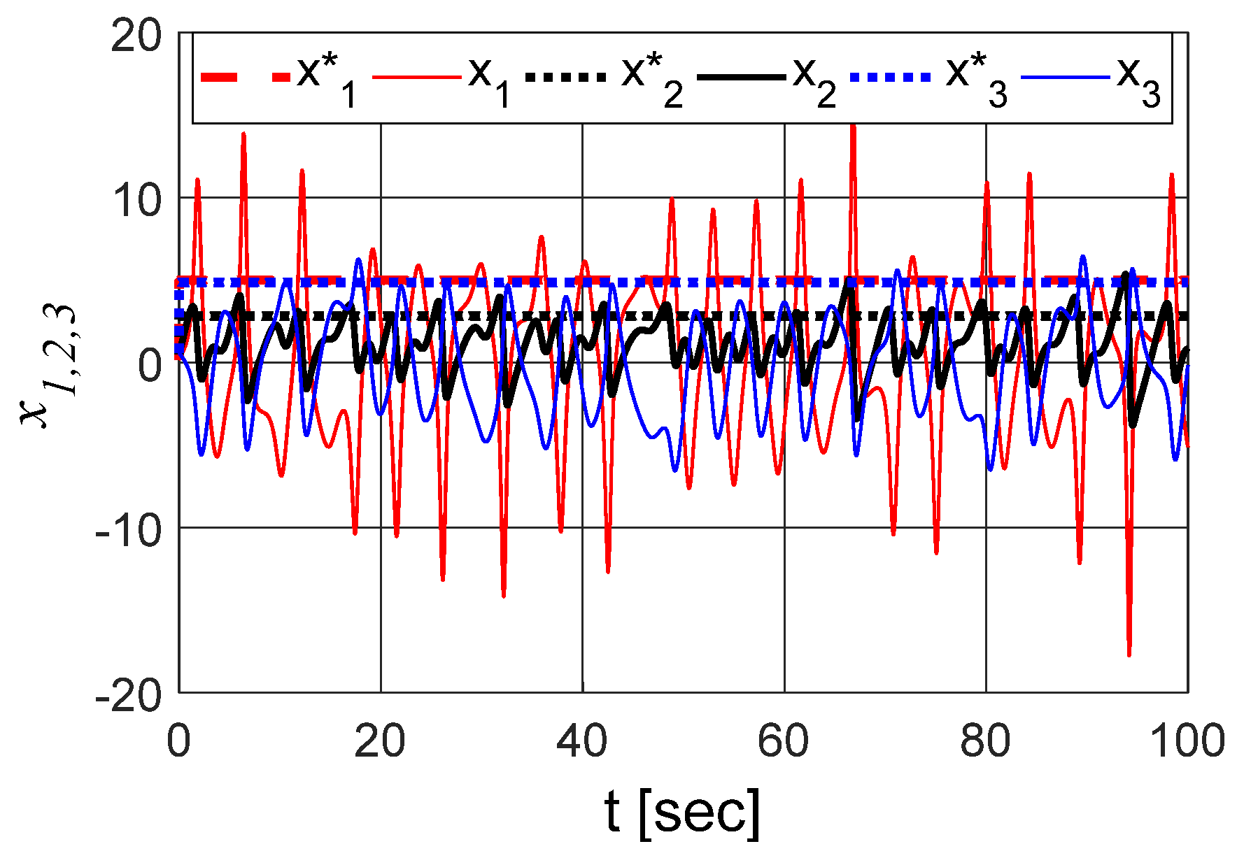
In Figure 7, we can observe the system without control and with control, where $x_1^{*}$, $x_2^{*}$, and $x_3^{*}$ are the controlled states $x_1$, $x_2$, and $x_3$, and are the states without control and with chaotic behavior.

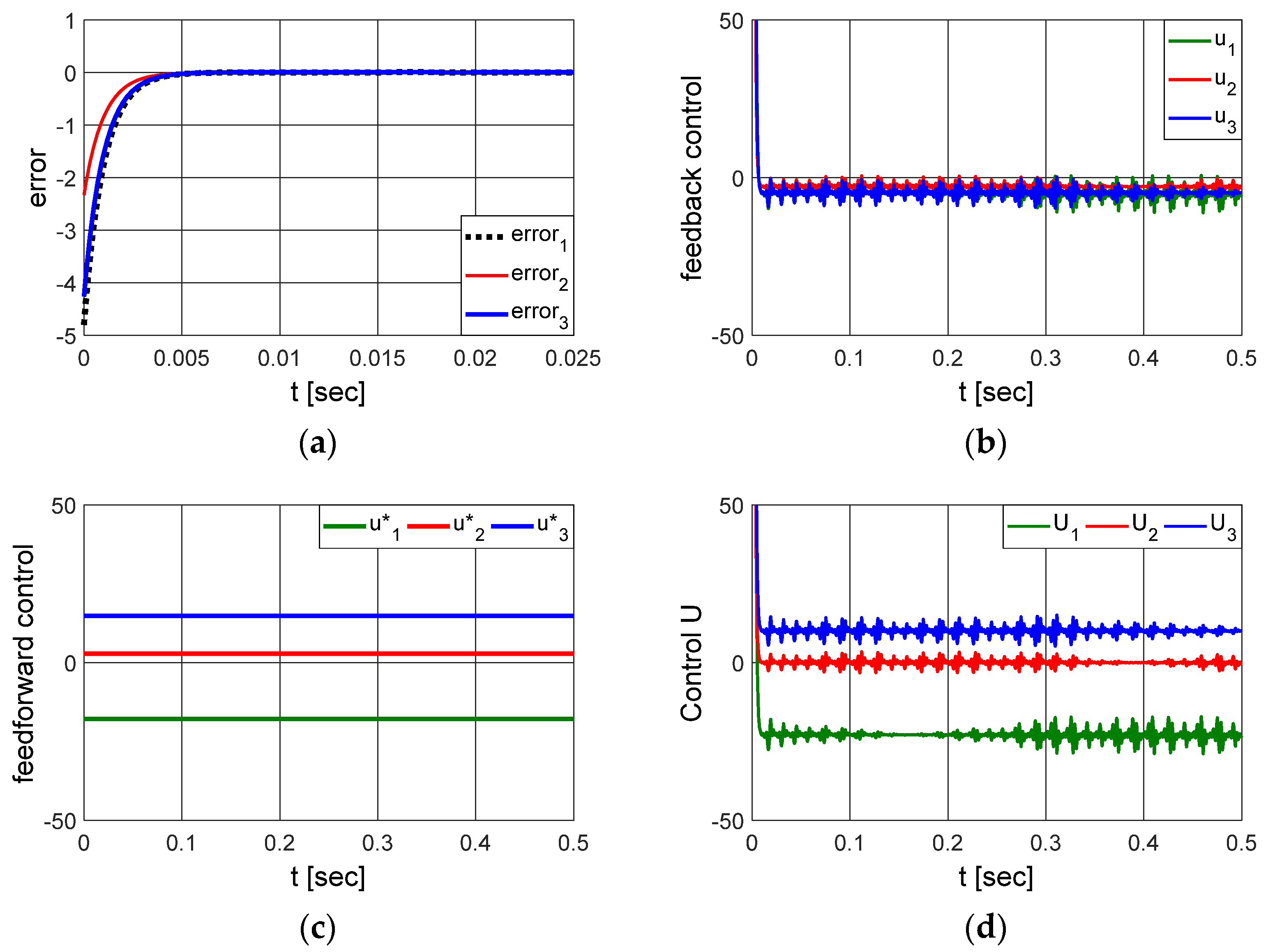
Figure 8 shows the control errors, the feedforward ($u^{*}$) and feedback ($u$) control signals, and the sum of the two control signals.

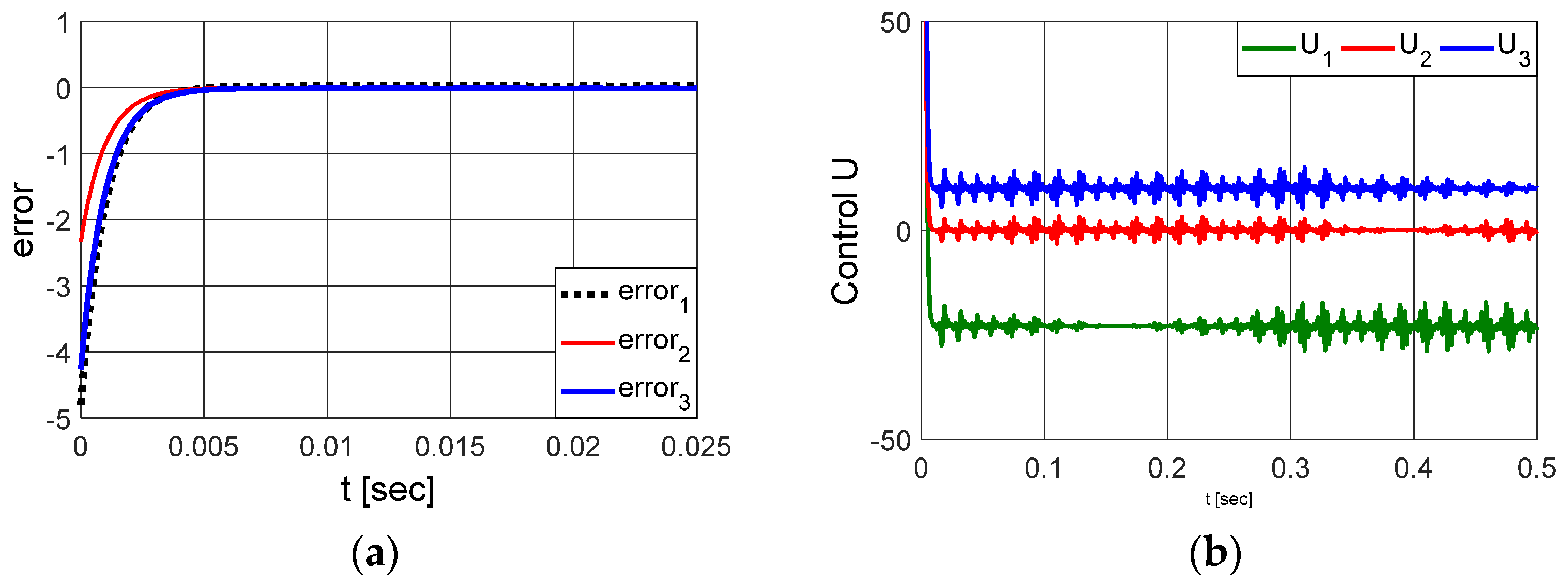
Figure 9 shows the error and the control signal for the case of using only the feedback control ($u$) obtained by the SDRE control.

Analyzing the results presented in Figure 8 and Figure 9, we verified that the combination of the feedback control ($u$) with the feedforward control ($u^{*}$) resulted in a reduced error in comparison to the system with only feedback control ($u$). The difference is practically imperceptible, since the error was below 0.1% in both cases. And, according to [43], errors of up to 2% can be considered acceptable, indicating that the proposed control exceeded the recommended rates. The error with the control $U=u+u^{*}$ was 21% smaller than the error obtained using the control $U=u$.

Parametric Sensitivity Analysis

To consider the effects of parameter uncertainties on the performance of the proposed control, we regarded that the parameters used in the control design as having a random error of 20%, a robustness analysis strategy similar to that used in [43].

The following parameters were used in the matrix $A$ (Equation (19)) and in the feedforward control ($u^{*}$, Equation (11)): $\mathrm{a}=0.24+0.12r(t)$, $b=0.008+0.004r(t)$, $c=0.8+0.4r(t)$, $d=0.04+0.02r(t)$, $e=2.064+1.032r(t)$, $f=1.68+0.84r(t)$, $g=0.8+0.4r(t)$, and $h=0.08+0.04r(t)$; $r(t)$ was a random function.

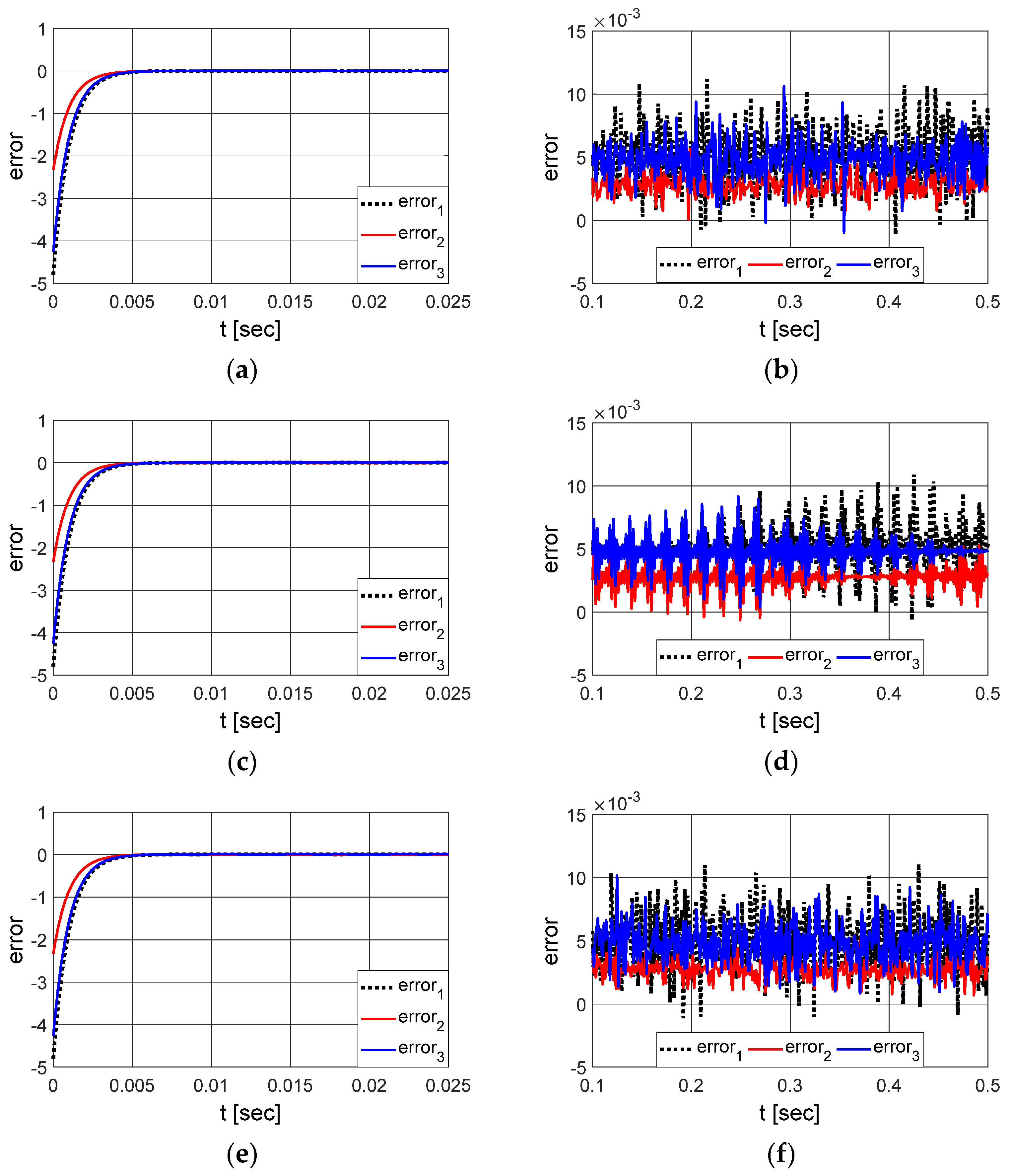
Figure 10 shows the robustness of the proposed control when the parameters utilized in the control had random uncertainties.

Analyzing the results presented in Figure 10, we can conclude that the proposed control is robust to parametric variations both for the feedback control ($u$) and for the feedback and feedforward combination ($U=u+u^{*}$), because the error was well below 2% for both cases, proving the robustness of the control for parameter errors.

3.2. Fractional Order System

We next considered the inclusion of the $U=u+u^{*}$ control in the system (3):

$$\begin{array}{l}\frac{d^{q_1}{x}_1}{d{t}^{q_1}}=f{x}_3+x_2{x}_1-a{x}_1+U_1\\ \frac{d^{q_2}{x}_2}{d{t}^{q_2}}=-b{x}_2^2-h{x}_1^2+e+U_2\\ \frac{d^{q_3}{x}_3}{d{t}^{q_3}}=-c{x}_3-g{x}_1-d{x}_2+U_3\end{array}$$

(20)

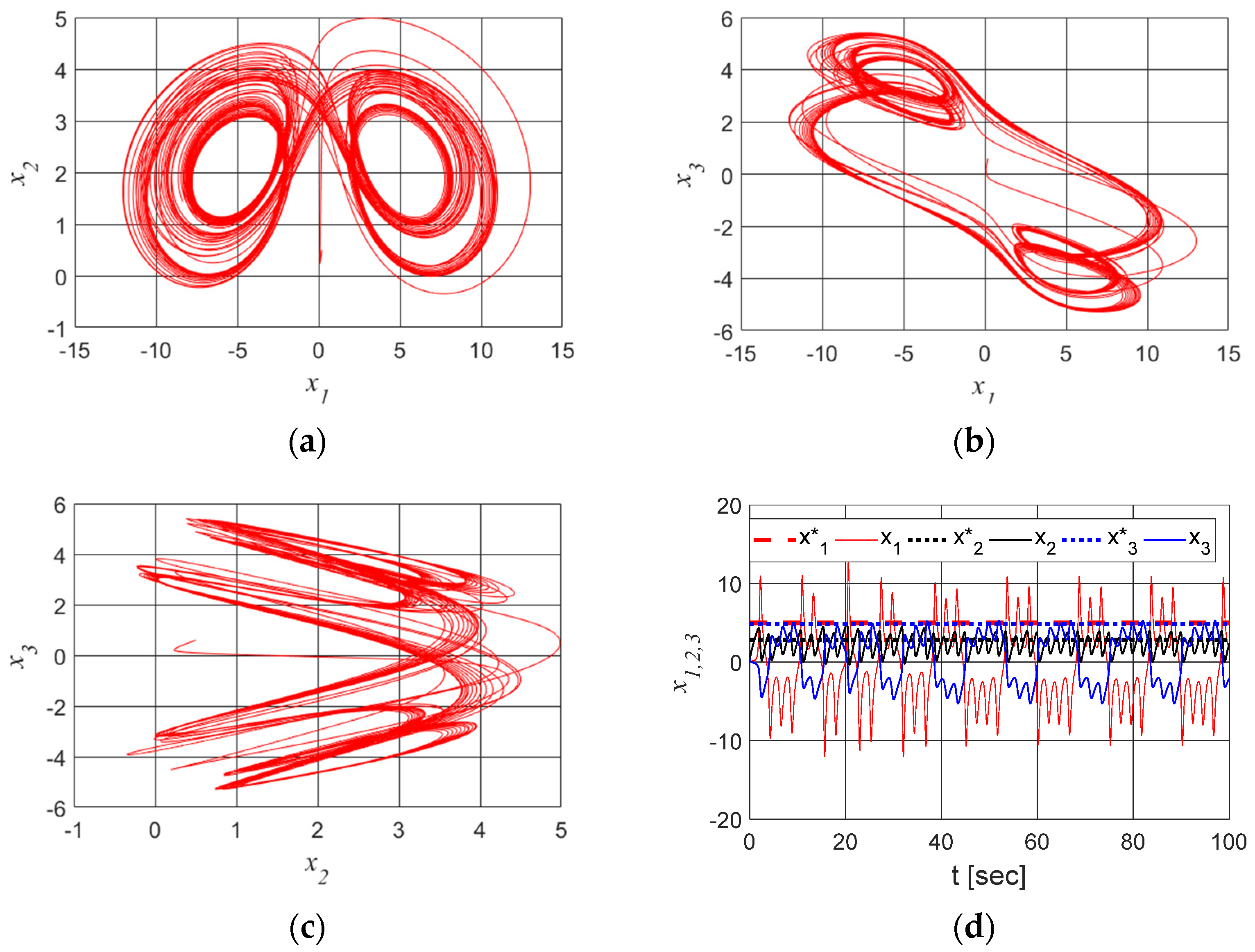
In Figure 11, we can observe the phase diagrams, the history in time for the system (21) with and without control, and the positioning errors for the proposed control, considering the case in which the system with the fractional order ($q_1=q_2=q_3=0.8$) has a chaotic behavior, as shown in Figure 6. $x_1^{*}$, $x_2^{*}$, and $x_3^{*}$ were the controlled states $x_1$, $x_2$ and $x_3$, and the states of the system without the control signal and with chaotic behavior, as seen in Figure 11a.

As shown in Figure 11, the proposed control is also efficient in controlling the financial system (1) in fractional order (3). The results showed that the steady-state error was well below 1%, demonstrating the robustness of the proposed control for variations in fractional order.

4. Conclusions

Integer and fractional order economic and financial systems with chaotic and hyperchaotic behavior were investigated, and a control design was proposed to suppress chaotic behavior. In this context, a numerical analysis was carried out to verify the influence of the system’s parameters on the economic and financial dynamics, proving that it is possible to obtain constant, periodic, chaotic, and hyperchaotic behaviors with proper adjustments of the parameters.

With the use of bifurcation diagrams and with the calculation of the Lyapunov exponent, the results presented make it possible to obtain a source of information for new research and economic and financial projects. These results indicate the trend of behavior as well as the maximums for each of the studied states.

In addition to studying the parameters’ influence on the system’s dynamics, a numerical analysis of the fractional order was included, using the 0-1 test to determine whether the system is chaotic. Numerical results demonstrated that the system becomes constant, periodic, or chaotic for specific values of the fractional order, and that economic and financial memory affect current and future results. Considering the negative factors that chaotic behavior can generate in economic and financial systems, the proposed control proved to be effective in suppressing chaotic behavior.

Parametric sensitivity analysis confirmed the proposed control’s robustness for integer and fractional orders. Numerical simulations also showed that it is possible to control the system only with the feedback control obtained by the suboptimal SDRE control. As a source of future work, a deeper analysis of the hyperchaotic behavior observed in this paper, both for integer and fractional orders, as well as other control techniques, can be highlighted. Other operators of the fractional order can also be considered, as well as using values of q > 1.

References

1. Tacha, O.I.; Munoz-Pacheco, J.M.; Zambrano-Serrano, E.; Stouboulos, I.N.; Pham, V.-T. Determining the chaotic behavior in a fractional-order finance system with negative parameters. Nonlinear Dyn. 2018, 94, 1303–1317. [Google Scholar] [CrossRef]
2. Stutzer, M.J. Chaotic Dynamics and bifurcation in a macro model. J. Econ. Dyn. Control 1980, 3, 353–376. [Google Scholar] [CrossRef] [Green Version]
3. Meyers, R.A. Complex Systems in Finance and Econometrics; Springer: New York, NY, USA, 2009. [Google Scholar]
4. Xu, C.; Aouiti, C.; Liao, M.; Li, P.; Liu, Z. Chaos control strategy for a fractional-order financial model. Adv. Differ. Equ. 2020, 2020, 573. [Google Scholar] [CrossRef]
5. Liao, Y.; Zhou, Y.; Xu, F.; Shu, X.-B. A Study on the Complexity of a New Chaotic Financial System. Complexity 2020, 2020, 8821156. [Google Scholar] [CrossRef]
6. Matrosov, V.V.; Shalfeev, V. Simulation of the Business-Cycle Synchronization Processes in an Ensemble of Coupled Economic Oscillators. Radiophys. Quantum. Electron. 2022, 64, 750–759. [Google Scholar] [CrossRef]
7. Dousseh, Y.P.; Monwanou, A.V.; Koukpémèdji, A.A.; Miwadinou, C.H.; Orou, J.B.C. Dynamics analysis, adaptive control, synchronization and anti-synchronization of a novel modified chaotic financial system. Int. J. Dynam. Control 2023, 11, 862–876. [Google Scholar] [CrossRef]
8. Fanti, L.; Manfredi, P. Chaotic business cycles and fiscal policy: An IS-LM model with distributed tax collection lags. Chaos Solitons Fractals 2007, 32, 736–744. [Google Scholar] [CrossRef]
9. Chian, A.L.; Rempel, E.L.; Rogers, C. Complex economic dynamics: Chaotic saddle, crisis and intermittency. Chaos Solitons Fractals 2006, 29, 1194–1218. [Google Scholar] [CrossRef]
10. Albulescu, C.T.; Tiwari, A.K.; Kyophilavong, P. Nonlinearities and Chaos: A New Analysis of CEE Stock Markets. Mathematics 2021, 9, 707. [Google Scholar] [CrossRef]
11. Inglada-Perez, L. A Comprehensive Framework for Uncovering Non-Linearity and Chaos in Financial Markets: Empirical Evidence for Four Major Stock Market Indices. Entropy 2020, 22, 1435. [Google Scholar] [CrossRef]
12. Cheng, H.; Huang, J.-B.; Guo, Y.-Q.; Zhu, X.-H. Long memory of price-volume correlation in metal futures market based on fractal features. Trans. Nonferrous Metals Soc. China 2013, 23, 3145–3152. [Google Scholar] [CrossRef]
13. David, S.A.; Machado, J.A.T.; Quintino, D.D.; Balthazar, J.M. Partial chaos suppression in a fractional order macroeconomic model. Math. Comput. Simul. 2016, 122, 55–68. [Google Scholar] [CrossRef] [Green Version]
14. Baskonus, H.M.; Mekkaoui, T.; Hammouch, Z.; Bulut, H. Active control of a chaotic fractional order economic system. Entropy 2015, 17, 5771–5783. [Google Scholar] [CrossRef] [Green Version]
15. Tacha, O.I.; Volos, C.K.; Kyprianidis, I.M.; Stouboulos, I.N.; Vaidyanathan, S.; Pham, V.T. Analysis, adaptive control and circuit simulation of a novel nonlinear finance system. Appl. Math. Comput. 2016, 276, 200–217. [Google Scholar] [CrossRef]
16. Xu, C.; Cui, X.; Li, P.; Yan, J.; Yao, L. Exploration on dynamics in a discrete predator–prey competitive model involving feedback controls. J. Biol. Dyn. 2023, 17, 2220349. [Google Scholar] [CrossRef]
17. Ou, W.; Xu, C.; Cui, Q.; Liu, Z.; Pang, Y.; Farman, M.; Ahmad, S.; Zeb, A. Mathematical study on bifurcation dynamics and control mechanism of tri-neuron bidirectional associative memory neural networks including delay. Math. Meth. Appl. Sci. 2023, 1, 1–25. [Google Scholar] [CrossRef]
18. Huang, C.; Liu, H.; Shi, X.; Chen, X.; Xiao, M.; Wang, Z.; Cao, J. Bifurcations in a fractional-order neural network with multiple leakage delays. Neural Netw. 2020, 131, 115–126. [Google Scholar] [CrossRef]
19. Huang, C.; Liu, H.; Chen, X.; Cao, J.; Alsaedi, A. Extended feedback and simulation strategies for a delayed fractional-order control system. Phys. A Stat. Mech. Its Appl. 2020, 545, 123127. [Google Scholar] [CrossRef]
20. Johansyah, M.D.; Sambas, A.; Mobayen, S.; Vaseghi, B.; Al-Azzawi, S.F.; Sukono; Sulaiman, I.M. Dynamical Analysis and Adaptive Finite-Time Sliding Mode Control Approach of the Financial Fractional-Order Chaotic System. Mathematics 2023, 11, 100. [Google Scholar] [CrossRef]
21. He, Y.; Peng, J.; Zheng, S. Fractional-Order Financial System and Fixed-Time Synchronization. Fractal Fract. 2022, 6, 507. [Google Scholar] [CrossRef]
22. Rao, R. Global Stability of a Markovian Jumping Chaotic Financial System with Partially Unknown Transition Rates under Impulsive Control Involved in the Positive Interest Rate. Mathematics 2019, 7, 579. [Google Scholar] [CrossRef] [Green Version]
23. Xin, B.; Li, Y. 0-1 Test for Chaos in a Fractional Order Financial System with Investment Incentive. Abstr. Appl. Anal. 2013, 2013, 876298. [Google Scholar] [CrossRef] [Green Version]
24. Chen, S.B.; Jahanshahi, H.; Abba, O.A.; Solís-Pérez, J.E.; Bekiros, S.; Gómez-Aguilar, J.F.; Yousefpour, A.; Chu, Y.M. The effect of market confidence on a financial system from the perspective of fractional calculus: Numerical investigation and circuit realization. Chaos Solitons Fractals 2020, 140, 110223. [Google Scholar] [CrossRef]
25. Yu, H.; Cai, G.; Li, Y. Dynamic analysis and control of a new hyperchaotic finance system. Chaos Solitons Fractals 2012, 45, 1048–1057. [Google Scholar] [CrossRef]
26. Yousefpour, A.; Jahanshahi, H.; Munoz-Pacheco, J.M.; Bekiros, S.; Wei, Z. A fractional-order hyper-chaotic economic system with transient chaos. Chaos Solitons Fractals 2020, 130, 109400. [Google Scholar] [CrossRef]
27. Cao, Y. Chaotic synchronization based on fractional order calculus financial system. Chaos Solitons Fractals 2020, 130, 109410. [Google Scholar] [CrossRef]
28. Gottwald, G.A.; Melbourne, I. A new test for chaos in deterministic systems. Proc. R. Soc. Lond. A Math. Phys. Eng. Sci. 2004, 460, 603–611. [Google Scholar] [CrossRef]
29. Tusset, A.M.; Ribeiro, M.A.; Lenz, W.B.; Rocha, R.T.; Balthazar, J.M. Time Delayed Feedback Control Applied in an Atomic Force Microscopy (AFM) Model in Fractional-Order. J. Vib. Eng. Technol. 2020, 8, 327–335. [Google Scholar] [CrossRef]
30. Tusset, A.M.; Balthazar, J.M.; Ribeiro, M.A.; Lenz, W.B.; Rocha, R.T. Chaos control of an atomic force microscopy model in fractional-order. Eur. Phys. J.-Spec. Top. 2021, 230, 3643–3654. [Google Scholar] [CrossRef]
31. Ribeiro, M.A.; Balthazar, J.M.; Lenz, W.B.; Rocha, R.T.; Tusset, A.M. Numerical Exploratory Analysis of Dynamics and Control of an Atomic Force Microscopy in Tapping Mode with Fractional Order. Shock. Vib. 2020, 2020, 4048307. [Google Scholar] [CrossRef]
32. Bassinello, D.G.; Tusset, A.M.; Rocha, R.T.; Balthazar, J.M. Dynamical Analysis and Control of a Chaotic Microelectromechanical Resonator Model. Shock. Vib. 2018, 2018, 4641629. [Google Scholar] [CrossRef] [Green Version]
33. Pearson, J.D. Approximation methods in optimal control. J. Electron. Control 1962, 13, 453–469. [Google Scholar] [CrossRef]
34. Tusset, A.M.; Balthazar, J.M.; Rocha, R.T.; Ribeiro, M.R.; Lenz, W.B. On suppression of chaotic motion of a nonlinear MEMS oscillator. Nonlinear Dyn. 2020, 99, 537–557. [Google Scholar] [CrossRef]
35. Wolf, A.; Swift, J.B.; Swinney, H.L.; Vastano, J.A. Determining Lyapunov exponents from a time series. Phys. D Nonlinear Phenom. 1985, 16, 285–317. [Google Scholar] [CrossRef] [Green Version]
36. Daũm, H.H.; Rocha, R.T.; Balthazar, J.M.; Tusset, A.M. Dynamic Analysis and Synchronization for a System with Hyperchaotic Behavior. Braz. J. Phys. 2021, 51, 1333–1345. [Google Scholar] [CrossRef]
37. Gao, Q.; Ma, J. Chaos and Hopf bifurcation of a finance system. Nonlinear Dyn. 2009, 58, 209–216. [Google Scholar] [CrossRef]
38. Petras, I. Fractional-Order Nonlinear Systems: Modeling, Analysis and Simulation; Springer Science & Business Media: Berlin/Heidelberg, Germany, 2011. [Google Scholar]
39. Günerhan, H.; Kaabar, M.K.A.; Çelik, E. Novel analytical and approximate-analytical methods for solving the nonlinear fractional smoking mathematical model. Sigma J. Eng. Nat. Sci. 2023, 41, 331–343. [Google Scholar] [CrossRef]
40. Gottwald, G.A.; Melbourne, I. Testing for chaos in deterministic systems with noise. Phys. D Nonlinear Phenom. 2005, 212, 100–110. [Google Scholar] [CrossRef] [Green Version]
41. Bernardini, D.; Litak, G. An overview of 0-1 test for chaos. J. Braz. Soc. Mech. Sci. Eng. 2016, 38, 1433–1450. [Google Scholar] [CrossRef]
42. Yuan, L.; Yang, Q.; Zeng, C. Chaos detection and parameter identification in fractional-order chaotic systems with delay. Nonlinear Dyn. 2013, 73, 439–448. [Google Scholar] [CrossRef]
43. Peruzzi, N.; Chavarette, F.; Balthazar, J.M.; Tusset, A.M.; Perticarrari, A.; Brasil, R. The dynamic behavior of a parametrically excited time-periodic MEMS taking into account parametric errors. J. Vib. Control 2016, 22, 4101–4110. [Google Scholar] [CrossRef]
Figure 1. First and second largest Lyapunov exponent. (a) First largest Lyapunov exponent for a = [ 0 : 1 ] versus b = [ 0 : 0.1 ] ; (b) second largest Lyapunov exponent for a = [ 0 : 1 ] versus b = [ 0 : 0.1 ] ; (c) first largest Lyapunov exponent for a = [ 0 : 1 ] versus c = [ 0.1 : 3 ] ; (d) second largest Lyapunov exponent for a = [ 0 : 1 ] versus c = [ 0.1 : 3 ] ; (e) first largest Lyapunov exponent for b = [ 0 : 0.1 ] versus c = [ 0.1 : 3 ] ; (f) second largest Lyapunov exponent for b = [ 0 : 0.1 ] versus c = [ 0.1 : 3 ] .
Fractalfract 07 00535 g001
Figure 2. First and second largest Lyapunov exponent. (a) First largest Lyapunov exponent for f = [ 0.1 : 3 ] versus e = [ 0.1 : 3 ] ; (b) second largest Lyapunov exponent for f = [ 0.1 : 3 ] versus e = [ 0.1 : 3 ] ; (c) first largest Lyapunov exponent for f = [ 0.1 : 3 ] versus g = [ 0.1 : 3 ] ; (d) second largest Lyapunov exponent for f = [ 0.1 : 3 ] versus g = [ 0.1 : 3 ] ; (e) first largest Lyapunov exponent for e = [ 0.1 : 3 ] versus g = [ 0.1 : 3 ] ; (f) second largest Lyapunov exponent for e = [ 0.1 : 3 ] versus g = [ 0.1 : 3 ] .
Fractalfract 07 00535 g002
Figure 3. (a) Time histories of the state x1; (b) time histories of the state x2; (c) time histories of the state x3.
Fractalfract 07 00535 g003
Figure 4. Phase diagrams. (a) x1 versus x2; (b) x1 versus x3; (c) x2 versus x3; (d) x1 versus x2 versus x3.
Fractalfract 07 00535 g004
Figure 5. Bifurcation diagrams. (a) a = [0:1] versus x1. (b) b = [0:1] versus x1. (c) c = [0.1:3] versus x1. (d) e = [0.1:3] versus x1. (e) f = [0.1:3] versus x1. (f) g = [0.1:3] versus x1.
Fractalfract 07 00535 g005
Figure 6. Time histories of state x 1 for q = [ 0.7 : 1 ] . (a) q = 0.7 . (b) q = 0.75 . (c) q = 0.80 . (d) q = 0.85 . (e) q = 0.9 . (f) q = 0.95 . (g) q = 1 .
Fractalfract 07 00535 g006aFractalfract 07 00535 g006b
Figure 7. Time histories of the states x1, x2, and x3 without control and x 1 * , x 2 * , and x 3 * with control.
Fractalfract 07 00535 g007
Figure 8. Time histories of the systems with control U = u + u * . (a) Errors e 1 = x 1 x 1 * , e 2 = x 2 x 2 * and e 3 = x 3 x 3 * . (b) Signal of feedback control by SDRE. (c) Signal of feedforward control. (d) Signal of feedback control + feedforward control ( U = u + u * ).
Fractalfract 07 00535 g008
Figure 9. Time histories of the systems with control U = u . (a) Errors e 1 = x 1 x 1 * , e 2 = x 2 x 2 * and e 3 = x 3 x 3 * . (b) Signal of the control ( u ) by SDRE.
Fractalfract 07 00535 g009
Figure 10. Errors e 1 = x 1 x 1 * , e 2 = x 2 x 2 * , and e 3 = x 3 x 3 * for uncertainty in parameters. (a,b) Uncertainty in parameters only of the feedforward control ( u * ). (c,d) Uncertainty in parameters only of the feedback control ( u ). (e,f) Uncertainty in the parameters of the feedforward control and feedback control ( U = u + u * ).
Fractalfract 07 00535 g010
Figure 11. (a) Phase diagrams x 1 versus x 2 . (b) Phase diagrams x 1 versus x 3 . (c) Phase diagrams x 2 versus x 3 . (d) Time histories of the states x 1 , x 2 , and x 3 without control and x 1 * , x 2 * , and x 3 * with control. (e,f) Errors e 1 = x 1 x ˜ 1 , e 2 = x 2 x ˜ 2 , and e 3 = x 3 x ˜ 3 .
Fractalfract 07 00535 g011aFractalfract 07 00535 g011b
Disclaimer/Publisher’s Note: The statements, opinions and data contained in all publications are solely those of the individual author(s) and contributor(s) and not of MDPI and/or the editor(s). MDPI and/or the editor(s) disclaim responsibility for any injury to people or property resulting from any ideas, methods, instructions or products referred to in the content.