The Evolution of COVID-19 Transmission with Superspreaders Class under Classical and Caputo Piecewise Operators: Real Data Perspective from India, France, and Italy

Abstract

In this study, we analyze the transmission of the COVID-19 model by using a piecewise operator in the classical Caputo sense. The existence along with the uniqueness of the solution of the COVID-19 model under a piecewise derivative is presented. The numerical scheme with Newton polynomials is used to obtain a numerical solution to the model under consideration. The graphical illustrations for the suggested model are demonstrated with various fractional orders. The crossover behavior of the considered system is observed in the graphical analysis. Furthermore, the comparison of simulations with real data for three different countries is presented, where best-fitted dynamics are observed.

1. Introduction

Since new coronavirus infections were predicted to increase by early March 2019, most likely via bats in China, no international preventive action was taken [1]. Following the discovery of a number of pneumonias of unknown origin, the National Health Commission of China provided additional details about the outbreak in early 2020 [2,3]. The outbreak is said to have begun at the Hunan fish market in Wuhan province, China. Despite the potential that COVID-19 clients in China consumed contaminated animals for food or visited the market, further examination indicated that the majority of people had not been to the fish store. As a result, it was determined that such a virus may spread from person to person through coughing, sneezing, and the emission of respiratory secretions or aerosols. Furthermore, virtually every country on every continent verified disease transmission caused by aerosols inhaled into the lungs and the upper respiratory system [4]. More than 10.27 million COVID-19-reported cases have been documented, and as of 30 June 2020, there have been more than 0.5 million fatalities worldwide [5]. America, Europe, Africa, and South-East Asia are the hardest afflicted by the coronavirus. Cough, temperature, exhaustion, and shortness of breath are the first signs of the COVID-19 virus. These symptoms develop between 2–10 days and can progress to cause pneumonia, renal failure, SARS, and even death [6]. Due to the lack of a vaccine and antiviral medications, the pandemic has continued to spread. As a result, the WHO declared it a worldwide concern. To minimize the propagation of infection, policymakers have developed non-medical interventions such as social isolation, self-quarantine, the isolation of diseased individuals, mask use, and safety equipment for medical staff. It was noted that an increasing number of nations began to impose travel restrictions abroad and close businesses, schools, and shopping centers. Globally, the 2019-nCoV pandemic has caused significant economic harm. Many medical professionals and academics worked tirelessly to fight the epidemic and carried out research in their fields of specialization. From various perspectives, including virology, bacterial infections, microbiology, veterinarian sciences, sociology, media studies, economics, etc., several authors examined 2019-nCoV.

Numerous mathematical models were proposed by researchers to evaluate the evolution behavior and propagation of the unique virus, which can aid in the prediction of future events and even the management of the COVID-19 outbreak [7,8]. Numerous mathematical models were constructed to investigate the transmission of COVID-19 dissemination patterns. These models give health authorities additional information about how to restrict the transmission of the illness [9]. Fanelli et al. [10] investigated a unique compartmental model that describes the COVID-19 spreading patterns in three nations with high infection rates. Ullah [11] investigated the propagation of COVID-19 with the influence of non-pharmaceutical therapies using data from Pakistan. A novel compartmentalized model for epidemiology was proposed by Alasmawi et al. [12] to account for the occurrence of certain people superspreading. They also propose a compartment for dying because of the viral disease.

The fractional order (FO) models help to comprehend the epidemic better and offer additional information. To mimic the spread of the coronavirus, fractional mathematical models, such as those in [13,14], are employed to represent the natural fact in a methodical manner. Various mathematical models utilizing differential operators that take into account nonlocality and the fading memory phenomena have been developed [15]. In comparison to the traditional integer order models [16], the non-integer order epidemiological systems are more accurate and useful for evaluating the behavior of an infectious illness [17,18]. Various disease models with fractional orders exhibit progressively greater matches to the real data. A different fractional operator is proposed in [19], and implementations of these fractional operators may be found in [20]. In addition, Ahmad et al. [21] examined the epidemiologic compartment model below in the Caputo fractional derivative, which would account for the superspreading behavior of some people. The model is given by [22]:

$$\begin{array}{ccc}\hfill \frac{d}{dt}\mathcal{S}\left(t\right)& =& -\mu \frac{I}{\mathrm{N}}\mathcal{S}-l\mu \frac{\mathcal{H}}{\mathrm{N}}\mathcal{S}-{\mu }^{{}^{\prime }}\frac{\mathcal{P}}{\mathrm{N}}\mathcal{S},\hfill \\ \hfill \frac{d}{dt}\mathcal{E}\left(t\right)& =& \mu \frac{I}{\mathrm{N}}\mathcal{S}+l\mu \frac{\mathcal{H}}{\mathrm{N}}\mathcal{S}+{\mu }^{{}^{\prime }}\frac{\mathcal{P}}{\mathrm{N}}\mathcal{S}-{\kappa }^{{}^{\prime }}\mathcal{E},\hfill \\ \hfill \frac{d}{dt}\mathcal{I}\left(t\right)& =& {\kappa }^{{}^{\prime }}{\sigma }_1\mathcal{E}-({\alpha }_a+{\alpha }_i)I-{\omega }_{i}I,\hfill \\ \hfill \frac{d}{dt}\mathcal{P}\left(t\right)& =& {\kappa }^{{}^{\prime }}{\sigma }_2\mathcal{E}-({\alpha }_a+{\alpha }_i)\mathcal{P}-{\omega }_{\mathcal{P}}\mathcal{P},\hfill \\ \hfill \frac{d}{dt}\mathcal{A}\left(t\right)& =& {\kappa }^{{}^{\prime }}(1-{\sigma }_1-{\rho }_2)\mathcal{E},\hfill \\ \hfill \frac{d}{dt}\mathcal{H}\left(t\right)& =& {\alpha }_a(I+\mathcal{P})-{\alpha }_r\mathcal{H}-{\omega }_h\mathcal{H},\hfill \\ \hfill \frac{d}{dt}\mathcal{R}\left(t\right)& =& {\alpha }_i(I+\mathcal{P})+{\alpha }_r\mathcal{H},\hfill \\ \hfill \frac{d}{dt}\mathcal{F}\left(t\right)& =& {\omega }_{i}I+{\omega }_{\mathcal{P}}\mathcal{P}+{\omega }_h\mathcal{H},\hfill \end{array}$$

(1)

subject to

$$\begin{array}{c}\hfill \left\{\begin{array}{c}\mathcal{S}\left(0\right)={\mathcal{S}}_0\ge 0,\mathcal{E}\left(0\right)={\mathcal{E}}_0\ge 0,\mathcal{I}\left(0\right)={\mathcal{I}}_0\ge 0,\mathcal{P}\left(0\right)={\mathcal{P}}_0\ge 0,\hfill \\ \mathcal{A}\left(0\right)={\mathcal{A}}_0\ge 0,\mathcal{H}\left(0\right)={\mathcal{H}}_0\ge 0,\mathcal{R}\left(0\right)={\mathcal{R}}_0\ge 0,\mathcal{F}\left(0\right)={\mathcal{F}}_0\ge 0.\hfill \end{array}\right.\end{array}$$

The whole population N is split into eight epidemiologic classes in this model: $\mathcal{S}$ denotes the susceptible populace, $\mathcal{E}$ represents exposed individuals, $\mathcal{I}$ is the symptomatic and infectious people, $\mathcal{P}$ provides the superspreader people, $\mathcal{A}$ denotes the infected but asymptomatic people, $\mathcal{H}$ gives the hospitalized populace, $\mathcal{R}$ provides the recovering populace, and $\mathcal{F}$ is the mortality class. When measuring the human–human infection coefficient, 0, 1 measure the aforementioned transmission coefficients of superspreader and hospitalized patients. For the speed with which a contagious individual exits the body after becoming symptomatic, superspreader, or asymptomatic, the exposed group is measured.

Recently, a new set of operators known as piecewise (PW) operators were introduced by Atangana et al. [23]. The Mittag–Leffler or exponential mappings cannot specify the timing of crossover. To address these issues, one of the novel methods of piecewise derivation has indeed been suggested in [23]. Researchers are currently studying crossover behaviors utilizing these operators in a different way; for instance, in [24,25], the authors studied different infectious disease models and qualitative features of DEs using these operators. Some more applications of piecewise operators are listed in [26,27,28,29]. Depending on these advantages, we will explore model (1) using the piecewise classical Caputo derivatives in the following manner:

$$\begin{array}{ccc}\hfill {}_0^{\mathrm{P}CC}{\mathrm{D}}_t^{\delta }\mathcal{S}\left(t\right)& =& -\mu \frac{I}{\mathrm{N}}\mathcal{S}-l\mu \frac{\mathcal{H}}{\mathrm{N}}\mathcal{S}-{\mu }^{{}^{\prime }}\frac{\mathcal{P}}{\mathrm{N}}\mathcal{S},\hfill \\ \hfill {}_0^{\mathrm{P}CC}{\mathrm{D}}_t^{\delta }\mathcal{E}\left(t\right)& =& \mu \frac{I}{\mathrm{N}}\mathcal{S}+l\mu \frac{\mathcal{H}}{\mathrm{N}}\mathcal{S}+{\mu }^{{}^{\prime }}\frac{\mathcal{P}}{\mathrm{N}}\mathcal{S}-{\kappa }^{{}^{\prime }}\mathcal{E},\hfill \\ \hfill {}_0^{\mathrm{P}CC}{\mathrm{D}}_t^{\delta }\mathcal{I}\left(t\right)& =& {\kappa }^{{}^{\prime }}{\sigma }_1\mathcal{E}-({\alpha }_a+{\alpha }_i)I-{\omega }_{i}I,\hfill \\ \hfill {}_0^{\mathrm{P}CC}{\mathrm{D}}_t^{\delta }\mathcal{P}\left(t\right)& =& {\kappa }^{{}^{\prime }}{\sigma }_2\mathcal{E}-({\alpha }_a+{\alpha }_i)\mathcal{P}-{\omega }_{\mathcal{P}}\mathcal{P},\hfill \\ \hfill {}_0^{\mathrm{P}CC}{\mathrm{D}}_t^{\delta }\mathcal{A}\left(t\right)& =& {\kappa }^{{}^{\prime }}(1-{\sigma }_1-{\rho }_2)\mathcal{E},\hfill \\ \hfill {}_0^{\mathrm{P}CC}{\mathrm{D}}_t^{\delta }\mathcal{H}\left(t\right)& =& {\alpha }_a(I+\mathcal{P})-{\alpha }_r\mathcal{H}-{\omega }_h\mathcal{H},\hfill \\ \hfill {}_0^{\mathrm{P}CC}{\mathrm{D}}_t^{\delta }\mathcal{R}\left(t\right)& =& {\alpha }_i(I+\mathcal{P})+{\alpha }_r\mathcal{H},\hfill \\ \hfill {}_0^{\mathrm{P}CC}{\mathrm{D}}_t^{\delta }\mathcal{F}\left(t\right)& =& {\omega }_{i}I+{\omega }_{\mathcal{P}}\mathcal{P}+{\omega }_h\mathcal{H}.\hfill \end{array}$$

(2)

In model (2), $\mathrm{P}CC$ stands for classical Caputo piecewise derivative. In a bit more detail, one can rewrite system (2) as:

$$\begin{array}{c}\hfill {}_0^{\mathrm{P}CC}{\mathrm{D}}_t^{\delta }\left(\mathcal{S}\left(t\right)\right)=\left\{\begin{array}{cc}& \frac{d}{dt}\left(\mathcal{S}\left(t\right)\right)={\mathfrak{F}}_1(\mathcal{S},t),0<t\le t_1,\hfill \\ & {}_0^C{\mathrm{D}}_t^{\delta }\left(\mathcal{S}\left(t\right)\right){=}^C{\mathfrak{F}}_1(\mathcal{S},t),t_1<t\le T,\hfill \end{array}\right.\\ \hfill {}_0^{\mathrm{P}CC}{\mathrm{D}}_t^{\delta }\left(\mathcal{E}\left(t\right)\right)=\left\{\begin{array}{cc}& \frac{d}{dt}\left(\mathcal{E}\left(t\right)\right)={\mathfrak{F}}_2(\mathcal{E},t),0<t\le t_1,\hfill \\ & {}_0^C{\mathrm{D}}_t^{\delta }\left(\mathcal{E}\left(t\right)\right){=}^C{\mathfrak{F}}_2(\mathcal{E},t),t_1<t\le T,\hfill \end{array}\right.\\ \hfill {}_0^{\mathrm{P}CC}{\mathrm{D}}_t^{\delta }\left(\mathcal{I}\left(t\right)\right)=\left\{\begin{array}{cc}& \frac{d}{dt}\left(\mathcal{I}\left(t\right)\right)={\mathfrak{F}}_3(\mathcal{I},t),0<t\le t_1,\hfill \\ & {}_0^C{\mathrm{D}}_t^{\delta }\left(\mathcal{I}\left(t\right)\right){=}^C{\mathfrak{F}}_3(\mathcal{I},t),t_1<t\le T,\hfill \end{array}\right.\\ \hfill {}_0^{\mathrm{P}CC}{\mathrm{D}}_t^{\delta }\left(\mathcal{P}\left(t\right)\right)=\left\{\begin{array}{cc}& \frac{d}{dt}\left(\mathcal{P}\left(t\right)\right)={\mathfrak{F}}_4(\mathcal{P},t),0<t\le t_1,\hfill \\ & {}_0^c{\mathrm{D}}_t^{\delta }\left(\mathcal{P}\left(t\right)\right){=}^C{\mathfrak{F}}_4(\mathcal{P},t),t_1<t\le T,\hfill \end{array}\right.\\ \hfill {}_0^{\mathrm{P}CC}{\mathrm{D}}_t^{\delta }\left(\mathcal{A}\left(t\right)\right)=\left\{\begin{array}{cc}& \frac{d}{dt}\left(\mathcal{A}\left(t\right)\right)={\mathfrak{F}}_5(\mathcal{A},t),0<t\le t_1,\hfill \\ & {}_0^C{\mathrm{D}}_t^{\delta }\left(\mathcal{A}\left(t\right)\right){=}^C{\mathfrak{F}}_5(\mathcal{A},t),t_1<t\le T,\hfill \end{array}\right.\\ \hfill {}_0^{\mathrm{P}CC}{\mathrm{D}}_t^{\delta }\left(\mathcal{H}\left(t\right)\right)=\left\{\begin{array}{cc}& \frac{d}{dt}\left(\mathcal{H}\left(t\right)\right)={\mathfrak{F}}_6(\mathcal{H},t),0<t\le t_1,\hfill \\ & {}_0^C{\mathrm{D}}_t^{\delta }\left(\mathcal{H}\left(t\right)\right){=}^C{\mathfrak{F}}_6(\mathcal{H},t),t_1<t\le T,\hfill \end{array}\right.\\ \hfill {}_0^{\mathrm{P}CC}{\mathrm{D}}_t^{\delta }\left(\mathcal{R}\left(t\right)\right)=\left\{\begin{array}{cc}& \frac{d}{dt}\left(\mathcal{R}\left(t\right)\right)={\mathfrak{F}}_7(\mathcal{R},t),0<t\le t_1,\hfill \\ & {}_0^C{\mathrm{D}}_t^{\delta }\left(\mathcal{R}\left(t\right)\right){=}^C{\mathfrak{F}}_7(\mathcal{R},t),t_1<t\le T,\hfill \end{array}\right.\\ \hfill {}_0^{\mathrm{P}CC}{\mathrm{D}}_t^{\delta }\left(\mathcal{F}\left(t\right)\right)=\left\{\begin{array}{cc}& \frac{d}{dt}\left(\mathcal{F}\left(t\right)\right)={\mathfrak{F}}_8(\mathcal{F},t),0<t\le t_1,\hfill \\ & {}_0^C{\mathrm{D}}_t^{\delta }\left(\mathcal{F}\left(t\right)\right){=}^C{\mathfrak{F}}_8(\mathcal{F},t),t_1<t\le T.\hfill \end{array}\right.\end{array}$$

(3)

2. Preliminaries

Here, some definitions of derivatives as well as integration will be portrayed in this section. Let FI and RL represent fractional integral and Reimann–Liouville, respectively.

Definition 1.

Consider $\mathit{V}\left(t\right)\in C[0,T]$ be a function, then the fractional order derivative in Caputo sense is given by:

$$\begin{array}{c}\hfill {}_0^{\mathrm{C}}{\mathrm{D}}_{\mathsf{t}}^{\delta }\mathit{V}\left(\mathsf{t}\right)=\frac{1}{\Gamma (1-\delta )}{\int }_0^{\mathsf{t}}{(\mathsf{t}-\mathrm{z})}^{-\delta }\frac{d}{dz}\mathit{V}\left(\mathrm{z}\right)d\mathrm{z}.\end{array}$$

Definition 2.

The RL FI is expressed as:

$$\begin{array}{c}\hfill {}_0^{\mathrm{RL}}{\mathrm{I}}_{\mathsf{t}}^{\delta }\mathit{V}\left(\mathsf{t}\right)=\frac{1}{\Gamma \left(\delta \right)}{\int }_0^{\mathsf{t}}{(\mathsf{t}-\mathrm{z})}^{\delta -1}\mathit{V}\left(\mathrm{z}\right)d\mathrm{z}.\end{array}$$

Definition 3

([23]). Consider that $\mathit{V}\left(\mathsf{t}\right)$ represents a PW continuous function, then integer order and FO PW derivative [23] may be expressed as:

$$\begin{array}{c}{}_0^{\mathrm{PCC}}{\mathrm{D}}_{\mathsf{t}}^{\delta }\mathit{V}\left(\mathsf{t}\right)=\left\{\begin{array}{cc}& \frac{d}{dt}\mathit{V}\left(t\right),0<t\le t_1,\hfill \\ & {}_0^{\mathrm{C}}{\mathrm{D}}_{\mathsf{t}}^{\delta }\mathit{V}\left(\mathsf{t}\right),{\mathsf{t}}_1<\mathsf{t}\le {\mathsf{t}}_2.\hfill \end{array}\right.\hfill \end{array}$$

Definition 4

([23]). Consider $\mathit{V}\left(\mathsf{t}\right)$ is a function, then the integer order and PW FI may be expressed as:

$$\begin{array}{c}\hfill {}_0^{\mathrm{P}F}{\mathrm{I}}_{\mathsf{t}}\mathit{V}\left(\mathsf{t}\right)=\left\{\begin{array}{cc}& {\int }_0^{\mathsf{t}}\mathit{V}\left(\mathrm{z}\right)d\mathrm{z},0<\mathsf{t}\le {\mathsf{t}}_1,\hfill \\ & \frac{1}{\Gamma \left(\delta \right)}{\int }_{{\mathsf{t}}_1}^{\mathsf{t}}{(\mathsf{t}-\mathrm{z})}^{\delta -1}U\left(\mathrm{z}\right)d\mathrm{z},{\mathsf{t}}_1<\mathsf{t}\le {\mathsf{t}}_2.\hfill \end{array}\right.\end{array}$$

Lemma 1

([23]). The equivalent form of a PW equation:

$$\begin{array}{c}\hfill {}_0^{\mathrm{PCC}}{\mathrm{D}}_{\mathsf{t}}^{\delta }\mathit{V}\left(\mathsf{t}\right)=G(\mathsf{t},\mathit{V}\left(\mathsf{t}\right)),0<\mathsf{t}\le 1,\end{array}$$

is given as:

$$\begin{array}{c}\hfill \mathit{V}\left(\mathsf{t}\right)=\left\{\begin{array}{cc}& {\mathit{V}}_0+{\int }_0^{\mathsf{t}}\mathit{V}\left(\mathrm{z}\right)d\mathrm{z},0<\mathsf{t}\le {\mathsf{t}}_1,\hfill \\ & \mathit{V}\left({\mathsf{t}}_1\right)+\frac{1}{\Gamma \left(\delta \right)}{\int }_{{\mathsf{t}}_1}^{\mathsf{t}}{(\mathsf{t}-\mathrm{z})}^{\delta -1}\mathit{V}\left(\mathrm{z}\right)d\mathrm{z},{\mathsf{t}}_1<\mathsf{t}\le {\mathsf{t}}_2.\hfill \end{array}\right.\end{array}$$

3. Existence and Uniqueness Results

The existence–uniqueness theory of the proposed PW COVID-19 model (2) in the piecewise notion is studied here. To do so, we can utilize the Lemma 1 and consider

$$\begin{array}{c}\hfill {}_0^{PCC}{D}_t^{\delta }\mathit{V}\left(t\right)=\mathfrak{F}(t,\mathit{V}),0<\delta \le 1.\end{array}$$

The equivalent form of the above equation is:

$$\begin{array}{c}\hfill \mathit{V}\left(t\right)=\left\{\begin{array}{c}{\mathit{V}}_0+{\int }_0^t\mathfrak{F}(\mathrm{z},\mathit{V}\left(\mathrm{z}\right))d\mathrm{z},0<t\le t_1,\hfill \\ \mathit{V}\left(t_1\right)+\frac{1}{\Gamma \left(\delta \right)}{\int }_{t_1}^{t_2}{(t-\mathrm{z})}^{\sigma -1}\mathfrak{F}(\mathrm{z},\mathit{V}\left(\mathrm{z}\right))d\mathrm{z}{t}_1<t\le t_2,\hfill \end{array}\right.\end{array}$$

(4)

where

$$\mathit{V}\left(t\right)=\left\{\begin{array}{cc}& \mathcal{S}\left(t\right)\hfill \\ & \mathcal{E}\left(t\right)\hfill \\ & \mathcal{I}\left(t\right)\hfill \\ & \mathcal{P}\left(t\right)\hfill \\ & \mathcal{A}\left(t\right)\hfill \\ & \mathcal{H}\left(t\right)\hfill \\ & \mathcal{R}\left(t\right)\hfill \\ & \mathcal{F}\left(t\right)\hfill \end{array}\right.,{\mathit{V}}_0=\left\{\begin{array}{cc}& \mathcal{S}\left(0\right)\hfill \\ & \mathcal{E}\left(0\right)\hfill \\ & \mathcal{I}\left(0\right)\hfill \\ & \mathcal{P}\left(0\right)\hfill \\ & \mathcal{A}\left(0\right)\hfill \\ & \mathcal{H}\left(0\right)\hfill \\ & \mathcal{R}\left(0\right)\hfill \\ & \mathcal{F}\left(0\right)\hfill \end{array}\right.,{\mathit{V}}_{t_1}=\left\{\begin{array}{cc}& {\mathcal{S}}_{\left(t_1\right)}\hfill \\ & {\mathcal{E}}_{t_1}\hfill \\ & {\mathcal{I}}_{\left(t_1\right)}\hfill \\ & {\mathcal{P}}_{t_1}\hfill \\ & {\mathcal{A}}_{t_1}\hfill \\ & {\mathcal{H}}_{t_1}\hfill \\ & {\mathcal{R}}_{t_1}\hfill \\ & {\mathcal{F}}_{\left(t_1\right)}\hfill \end{array}\right.,\mathfrak{F}(t,\mathit{V}\left(t\right))=\left\{\begin{array}{c}\hfill {\mathfrak{F}}_1=\left\{\begin{array}{cc}& \frac{d}{dt}{\mathfrak{F}}_1(\mathcal{S},t)\hfill \\ & {}^C{\mathfrak{F}}_1(\mathcal{S},t)\hfill \end{array}\right.\\ \hfill {\mathfrak{F}}_2=\left\{\begin{array}{cc}& \frac{d}{dt}{\mathfrak{F}}_2(\mathcal{E},t)\hfill \\ & {}^C{\mathfrak{F}}_2(\mathcal{E},t)\hfill \end{array}\right.\\ \hfill {\mathfrak{F}}_3=\left\{\begin{array}{cc}& \frac{d}{dt}{\mathfrak{F}}_3(\mathcal{I},t)\hfill \\ & {}^C{\mathfrak{F}}_3(\mathcal{I},t)\hfill \end{array}\right.\\ \hfill {\mathfrak{F}}_4=\left\{\begin{array}{cc}& \frac{d}{dt}{\mathfrak{F}}_4(\mathcal{P},t)\hfill \\ & {}^C{\mathfrak{F}}_4(\mathcal{P},t)\hfill \end{array}\right.\\ \hfill {\mathfrak{F}}_5=\left\{\begin{array}{cc}& \frac{d}{dt}{\mathfrak{F}}_5(\mathcal{A},t)\hfill \\ & {}^C{\mathfrak{F}}_5(\mathcal{A},t)\hfill \end{array}\right.\\ \hfill {\mathfrak{F}}_6=\left\{\begin{array}{cc}& \frac{d}{dt}{\mathfrak{F}}_6(\mathcal{H},t)\hfill \\ & {}^C{\mathfrak{F}}_6(\mathcal{H},t)\hfill \end{array}\right.\\ \hfill {\mathfrak{F}}_7=\left\{\begin{array}{cc}& \frac{d}{dt}{\mathfrak{F}}_7(\mathcal{R},t)\hfill \\ & {}^C{\mathfrak{F}}_7(\mathcal{R},t)\hfill \end{array}\right.\\ \hfill {\mathfrak{F}}_8=\left\{\begin{array}{cc}& \frac{d}{dt}{\mathfrak{F}}_8(\mathcal{F},t)\hfill \\ & {}^C{\mathfrak{F}}_8(\mathcal{F},t)\hfill \end{array}\right.\end{array}\right..$$

(5)

Taking $\infty >t_2\ge t>t_1>0$ and Banach space $E_1=C[0,T]$ with norm:

$$\parallel \mathit{V}\parallel =\underset{t\in [0,T]}{max}\left|\mathit{V}\left(t\right)\right|.$$

Here, we consider the Lipschitz and growth conditions in the form as follows:

(C1)

∃$L_{\mathit{V}}>0$, ∀$\mathit{V},\overline{\mathit{V}}\in E$, so that

$$|\mathfrak{F}(t,\mathit{V})-\mathfrak{F}(t,\overline{\mathit{V}})|\le L_{\mathfrak{F}}|\mathit{V}-\overline{\mathit{V}}|.$$

(C2)

∃$C_{\mathfrak{F}}>0$&$M_{\mathfrak{F}}>0,$ so that

$$\left|\mathfrak{F}(t,\mathit{V}\left(t\right))\right|\le C_{\mathfrak{F}}\left|\mathit{V}\right|+M_{\mathfrak{F}}.$$

Theorem 1.

If $\mathfrak{F}$ is a function which is PW continuous on $t\in [0,t_1]$ and $t_1<t\le t_2$ on $[0,T]$, and assuming $\left(C2\right)$, then Equation (4) has at least one solution.

Proof. 

Consider a closed subset as B of E in the two subintervals of $[0,T]$ by

$$B=\{\mathit{V}\in E:\parallel \mathit{V}\parallel \le R_{1,2},R>0\}.$$

Let us define $\mathbb{T}:B\to B$ by using (13) as

$$\begin{array}{c}\hfill \mathbb{T}\left(\mathit{V}\right)=\left\{\begin{array}{c}{\mathit{V}}_0+{\int }_0^t\mathfrak{F}(\mathrm{z},\mathit{V}\left(\mathrm{z}\right))d\mathrm{z},0<t\le t_1,\hfill \\ \mathit{V}\left(t_1\right)+\frac{1}{\Gamma \left(\delta \right)}{\int }_{t_1}^{t_2}{(t-\mathrm{z})}^{\sigma -1}\mathfrak{F}(\mathrm{z},\mathit{V}\left(\mathrm{z}\right))d\mathrm{z},t_1<t\le t_2.\hfill \end{array}\right.\end{array}$$

(6)

For any $\mathit{V}\in B$, one reach:

$$\begin{array}{ccc}\hfill \left|\mathbb{T}\right(\mathit{V}\left)\right(t\left)\right|& \le & \left\{\begin{array}{c}|{\mathit{V}}_0|+{\int }_0^{t_1}\left|\mathfrak{F}(\mathrm{z},\mathit{V}\left(\mathrm{z}\right))\right|d\mathrm{z},\hfill \\ |{\mathit{V}}_{(}{t}_1\left)\right|+\frac{1}{\Gamma \left(\delta \right)}{\int }_{t_1}^{t_2}{(t-\mathrm{z})}^{\delta -1}\left|\mathfrak{F}\left(\mathrm{z}\mathit{V}\left(\mathrm{z}\right)\right)\right|d\mathrm{z},\hfill \end{array}\right.\hfill \\ & \le & \left\{\begin{array}{c}|{\mathit{V}}_0|+{\int }_0^{t_1}[C_{\mathfrak{F}}\left|\mathit{V}\right|+M_{\mathfrak{F}}]d\mathrm{z},\hfill \\ |{\mathit{V}}_{(}{t}_1\left)\right|+\frac{1}{\Gamma \left(\delta \right)}{\int }_{t_1}^{t_2}{(t-\mathrm{z})}^{\delta -1}[C_{\mathfrak{F}}\left|\mathit{V}\right|+M_{\mathfrak{F}}]d\mathrm{z},\hfill \end{array}\right.\hfill \\ & \le & \left\{\begin{array}{c}|{\mathit{V}}_0|+{\mathrm{t}}_1[C_{\mathfrak{F}}\left|\mathit{V}\right|+M_{\mathfrak{F}}]=R_1,0<t\le t_1,\hfill \\ |{\mathit{V}}_{(}{t}_1\left)\right|+\frac{{({\mathrm{t}}_2-{\mathrm{t}}_1)}^{\delta }}{\Gamma (\delta +1)}[C_{\mathfrak{F}}\left|\mathrm{g}\right|+M_{\mathfrak{F}}]=R_2,t_1<t\le t_2,\hfill \end{array}\right.\hfill \\ & \le & \left\{\begin{array}{c}{R}_1,0<t\le t_1,\hfill \\ R_2,t_1<t\le t_2.\hfill \end{array}\right.\hfill \end{array}$$

As shown by the preceding equation, $\mathit{V}\in B$. As a result, $\mathbb{T}\left(B\right)$⊆B. As more than just a result, it establishes that $\mathbb{T}$ is closed as well as complete. We can write to further demonstrate the complete continuity of $\mathbb{T}$. Consider $t_m<t_n\in [0,t_1]$ as the beginning interval again for the integer order operator as:

$$\begin{array}{ccc}\hfill |\mathbb{T}\left(\mathit{V}\right)\left(t_n\right)-\mathbb{T}\left(\mathrm{g}\right)\left(t_m\right)|& =& |{\int }_0^{t_n}\mathfrak{F}(\mathrm{z},\mathit{V}\left(\mathrm{z}\right))d\mathrm{z}\hfill \\ & -& {\int }_0^{t_m}\mathfrak{F}(\mathrm{z},\mathrm{g}\left(\mathrm{z}\right))d\mathrm{z}|\hfill \\ & \le & {\int }_0^{t_n}\left|\mathfrak{F}(\mathrm{z},\mathit{V}\left(\mathrm{z}\right))\right|d\mathrm{z}\hfill \\ & -& {\int }_0^{t_m}\left|\mathfrak{F}(\mathrm{z},\mathrm{g}\left(\mathrm{z}\right))\right|d\mathrm{z}\hfill \\ & \le & [{\int }_0^{t_n}(C_{\mathfrak{F}}\left|\mathit{V}\right|+M_{\mathfrak{F}})\hfill \\ & -& {\int }_0^{t_m}(C_{\mathfrak{F}}\left|\mathrm{g}\right|+M_{\mathfrak{F}})]\hfill \\ & \le & (C_{\mathfrak{F}}\mathit{V}+M_{\mathfrak{F}})[t_n-t_m].\hfill \end{array}$$

(7)

Thanks to (7), one may obtain:

$$|\mathbb{T}\left(\mathit{V}\right)\left(t_n\right)-\mathbb{T}\mathrm{g}\left(t_m\right)|\to 0,\mathrm{as}{t}_m\mathrm{approaches}{t}_n.$$

Thus, it shows that the aforesaid operator $\mathbb{T}$ is equicontinuous on $[0,t_1]$. Consider $t_i,t_j\in [t_1,T]$ in the sense of Caputo as:

$$\begin{array}{ccc}\hfill |\mathbb{T}\left(\mathit{V}\right)\left(t_n\right)-\mathbb{T}\left(\mathit{V}\right)\left(t_m\right)|& =& |\frac{1}{\Gamma \left(\delta \right)}{\int }_0^{t_n}{(t_n-\mathrm{z})}^{\delta -1}\mathfrak{F}\left(\mathrm{z}\mathit{V}\left(\mathrm{z}\right)\right)d\mathrm{z}\hfill \\ & -& \frac{1}{\Gamma \left(\delta \right)}{\int }_0^{t_m}{(t_m-\mathrm{z})}^{\delta -1}\mathfrak{F}(\mathrm{z},\mathit{V}\left(\mathrm{z}\right))d\mathrm{z}|\hfill \\ & \le & \frac{1}{\Gamma \left(\delta \right)}{\int }_0^{t_m}[{(t_m-\mathrm{z})}^{\delta -1}-{(t_n-\mathrm{z})}^{\delta -1}]\left|\mathfrak{F}(\mathrm{z},\mathit{V}\left(\mathrm{z}\right))\right|d\mathrm{z}\hfill \\ & +& \frac{1}{\Gamma \left(\delta \right)}{\int }_{t_m}^{t_n}{(t_n-\mathrm{z})}^{\delta -1}\left|G(\mathrm{z},\mathit{V}\left(\mathrm{z}\right))\right|d\mathrm{z}\hfill \\ & \le & \frac{1}{\Gamma \left(\delta \right)}[{\int }_0^{t_m}[{(t_m-\mathrm{z})}^{\delta -1}-{(t_n-\mathrm{z})}^{\delta -1}]d\mathrm{z}\hfill \\ & +& {\int }_{t_m}^{t_n}{(t_n-\mathrm{z})}^{\delta -1}d\mathrm{z}](C_{\mathfrak{F}}\left|\mathit{V}\right|+M_{\mathfrak{F}})\hfill \\ & \le & \frac{(C_{\mathfrak{F}}\mathit{V}+M_{\mathfrak{F}})}{\Gamma (\delta +1)}[t_n^{\delta }-t_m^{\delta }+2{(t_n-t_m)}^{\delta }].\hfill \end{array}$$

(8)

If $t_n\to {\mathsf{t}}_m$, then

$$|\mathbb{T}\left(\mathit{V}\right)\left(t_n\right)-\mathbb{T}\left(\mathit{V}\right)\left(t_m\right)|\to 0.$$

These show the equicontinuity of $\mathbb{T}$ in $[t_1,t_2]$. As a result, $\mathbb{T}$ is an equicontinuous map. Then, we can say that $\mathbb{T}$ is completely continuous, uniformly continuous, and bounded as well, in the view of the Arzelà–Ascoli result. According to the Schauder result, the piecewise COVID-19 model (4) has at least a single solution on each subinterval.    □

Theorem 2.

Consider $\left(C1\right)$; the proposed PW COVID-19 model has at most a single solution if $\mathbb{T}$ satisfies the contraction criteria.

Proof. 

As $\mathbb{T}:B\to B$ PW continuous, consider $\mathit{V}$ and $\overline{\mathit{V}}\in B$ on $[0,t_1]$ in the classical sense as:

$$\begin{array}{ccc}\hfill \parallel \mathbb{T}\left(\mathit{V}\right)-\mathbb{T}\left(\overline{\mathit{V}}\right)\parallel & =& \underset{t\in [0,t_1]}{max}|{\int }_0^{t_1}\mathfrak{F}(\mathrm{z},\mathit{V}\left(\mathrm{z}\right))d\mathrm{z}-{\int }_0^{t_1}\mathfrak{F}(\mathrm{z},\overline{\mathit{V}}\left(\mathrm{z}\right))d\mathrm{z}|\hfill \\ & \le & t_1{L}_{\mathfrak{F}}\parallel \mathit{V}-\overline{\mathit{V}}\parallel .\hfill \end{array}$$

(9)

From (9), we attain

$$\begin{array}{c}\hfill \parallel \mathbb{T}\left(\mathit{V}\right)-\mathbb{T}\left(\overline{\mathit{V}}\right)\parallel \le t_1{L}_{\mathfrak{F}}\parallel \mathit{V}-\overline{\mathit{V}}\parallel .\end{array}$$

(10)

Hence, $\mathbb{T}$ is a contraction. Thus, the problem under study has a single solution only in the subinterval according to the Banach result. Further, for $t\in [t_1,t_2]$, we have

$$\begin{array}{ccc}\hfill \parallel \mathbb{T}\left(\mathit{V}\right)-\mathbb{T}\left(\overline{\mathit{V}}\right)\parallel & =& \underset{t\in [t_1,t_2]}{max}|\frac{1}{\Gamma \left(\delta \right)}{\int }_{t_1}^{t_2}{(t-\mathrm{z})}^{\delta -1}\mathfrak{F}(\mathrm{z},\mathit{V}\left(\mathrm{z}\right))d\mathrm{z}-\frac{1}{\Gamma \left(\delta \right)}{\int }_{t_1}^{t_2}{(t-\mathrm{z})}^{\delta -1}\mathfrak{F}(\mathrm{z},\overline{\mathit{V}}\left(\mathrm{z}\right))d\mathrm{z}|\hfill \\ & \le & \frac{{(t_2-t_1)}^{\delta }}{\Gamma (\delta +1)}{L}_{\mathfrak{F}}\parallel \mathit{V}-\overline{\mathit{V}}\parallel .\hfill \end{array}$$

(11)

From (11), it follows that

$$\begin{array}{c}\hfill \parallel \mathbb{T}\left(\mathit{V}\right)-\mathbb{T}\left(\overline{\mathit{V}}\right)\parallel \le \frac{{(t_2-t_1)}^{\delta }}{\Gamma (\delta +1)}{L}_{\mathfrak{F}}\parallel \mathit{V}-\overline{\mathit{V}}\parallel .\end{array}$$

(12)

Hence, $\mathbb{T}$ is a contraction. Thus, the problem under study has a single solution only in the subinterval according to the Banach result. As a result, the proposed PW system has a unique solution on every subinterval.    □

4. Numerical Results

Here, we derive a numerical scheme to analyze the PW model (2). Applying the piecewise integral to Equation (3), we have

$$\begin{array}{ccc}\hfill \mathcal{S}\left(t\right)& =& \left\{\begin{array}{c}{\mathcal{S}}_0+{\int }_0^{t_1}{\mathfrak{F}}_1(\mathrm{z},\mathcal{S})d\mathrm{z},0<t\le t_1,\hfill \\ \mathcal{S}\left(t_1\right)+\frac{1}{\Gamma \left(\delta \right)}{\int }_{t_1}^{t_2}{(t-\mathrm{z})}^{\delta -1}{\mathfrak{F}}_1(\mathrm{z},\mathcal{S})d\mathrm{z},t_1<t\le t_2,\hfill \end{array}\right.\hfill \\ \hfill \mathcal{E}\left(t\right)& =& \left\{\begin{array}{c}{\mathcal{E}}_0+{\int }_0^{t_1}{\mathfrak{F}}_2(\mathrm{z},\mathcal{E})d\mathrm{z},0<t\le t_1,\hfill \\ \mathcal{E}\left(t_1\right)+\frac{1}{\Gamma \left(\delta \right)}{\int }_{t_1}^{t_2}{(t-\mathrm{z})}^{\delta -1}{\mathfrak{F}}_2(\mathrm{z},\mathcal{E})d\mathrm{z},t_1<t\le t_2,\hfill \end{array}\right.\hfill \\ \hfill \mathcal{I}\left(t\right)& =& \left\{\begin{array}{c}{\mathcal{I}}_0+{\int }_0^{t_1}{\mathfrak{F}}_3(\mathrm{z},\mathcal{I})d\mathrm{z},0<t\le t_1,\hfill \\ \mathcal{I}\left(t_1\right)+\frac{1}{\Gamma \left(\delta \right)}{\int }_{t_1}^{t_2}{(t-\mathrm{z})}^{\delta -1}{\mathfrak{F}}_3(\mathrm{z},\mathcal{I})d\mathrm{z},t_1<t\le t_2,\hfill \end{array}\right.\hfill \\ \hfill \mathcal{P}\left(t\right)& =& \left\{\begin{array}{c}{\mathcal{P}}_0+{\int }_0^{t_1}{\mathfrak{F}}_4(\mathrm{z},\mathcal{P})d\mathrm{z},0<t\le t_1,\hfill \\ \mathcal{P}\left(t_1\right)+\frac{1}{\Gamma \left(\delta \right)}{\int }_{t_1}^{t_2}{(t-\mathrm{z})}^{\delta -1}{\mathfrak{F}}_4(\mathrm{z},\mathcal{P})d\mathrm{z},t_1<t\le t_2,\hfill \end{array}\right.\hfill \\ \hfill \mathcal{A}\left(t\right))& =& \left\{\begin{array}{c}{\mathcal{A}}_0+{\int }_0^{t_1}{\mathfrak{F}}_5(\mathrm{z},\mathcal{A})d\mathrm{z},0<t\le t_1,\hfill \\ \mathcal{A}\left(t_1\right)+\frac{1}{\Gamma \left(\delta \right)}{\int }_{t_1}^{t_2}{(t-\mathrm{z})}^{\delta -1}{\mathfrak{F}}_5(\mathrm{z},\mathcal{A})d\mathrm{z},t_1<t\le t_2,\hfill \end{array}\right.\hfill \\ \hfill \mathcal{H}\left(t\right)& =& \left\{\begin{array}{c}{\mathcal{H}}_0+{\int }_0^{t_1}{\mathfrak{F}}_6(\mathrm{z},\mathcal{H})d\mathrm{z},0<t\le t_1,\hfill \\ \mathcal{H}\left(t_1\right)+\frac{1}{\Gamma \left(\delta \right)}{\int }_{t_1}^{t_2}{(t-\mathrm{z})}^{\delta -1}{\mathfrak{F}}_6(\mathrm{z},\mathcal{H})d\mathrm{z},t_1<t\le t_2,\hfill \end{array}\right.\hfill \\ \hfill \mathcal{R}\left(t\right)& =& \left\{\begin{array}{c}{\mathcal{R}}_0+{\int }_0^{t_1}{\mathfrak{F}}_7(\mathrm{z},\mathcal{R})d\mathrm{z},0<t\le t_1,\hfill \\ \mathcal{R}\left(t_1\right)+\frac{1}{\Gamma \left(\delta \right)}{\int }_{t_1}^{t_2}{(t-\mathrm{z})}^{\delta -1}{\mathfrak{F}}_7(\mathrm{z},\mathcal{R})d\mathrm{z},t_1<t\le t_2,\hfill \end{array}\right.\hfill \\ \hfill \mathcal{F}\left(t\right)& =& \left\{\begin{array}{c}{\mathcal{F}}_0+{\int }_0^{t_1}{\mathfrak{F}}_8(\mathrm{z},\mathcal{F})d\mathrm{z},0<t\le t_1,\hfill \\ \mathcal{F}\left(t_1\right)+\frac{1}{\Gamma \left(\delta \right)}{\int }_{t_1}^{t_2}{(t-\mathrm{z})}^{\delta -1}{\mathfrak{F}}_8(\mathrm{z},\mathcal{F})d\mathrm{z},t_1<t\le t_2.\hfill \end{array}\right.\hfill \end{array}$$

(13)

At $t=t_{n+1}$, and for step size $\mathrm{h}$, we prove present the scheme for Equation (13). Now, Equation (13) can be expressed with Newton interpolation presented in [23] as:

$$\begin{array}{c}\hfill \mathcal{S}\left(t_{n+1}\right)=\left\{\begin{array}{c}\mathcal{S}\left(0\right)+\left\{\begin{array}{c}\sum _{\mathrm{K}=2}^i\left[\frac{5}{12}{\mathfrak{F}}_1({\mathbb{U}}_2,t_{\mathrm{K}-2})\mathrm{h}-\frac{4}{3}{\mathfrak{F}}_1({\mathbb{U}}_1,t_{\mathrm{K}-1})\mathrm{h}+{\mathfrak{F}}_1(\mathbb{U},t_{\mathrm{K}})\right],\hfill \end{array}\right.\hfill \\ \mathcal{S}\left(t_1\right)+\left\{\begin{array}{c}\frac{{\mathrm{h}}^{\delta -1}}{\Gamma (\delta +1)}\sum _{\mathrm{K}=i+3}^n\left[{\mathfrak{F}}_1({\mathbb{U}}_2,t_{\mathrm{K}-2})\right]\Pi \hfill \\ +\frac{{\mathrm{h}}^{\delta -1}}{\Gamma (\delta +2)}\sum _{\mathrm{K}=i+3}^n\left[{\mathfrak{F}}_1({\mathbb{U}}_1,t_{\mathrm{K}-1})-{\mathfrak{F}}_1({\mathbb{U}}_2,t_{\mathrm{K}-2})\right]\Theta \hfill \\ +\frac{\delta {\mathrm{h}}^{\delta -1}}{2\Gamma (\delta +3)}\sum _{\mathrm{K}=i+3}^n\left[{\mathfrak{F}}_1(\mathbb{U},t_{\mathrm{K}})-2G_2({\mathbb{U}}_1,t_{\mathrm{K}-1})+{\mathfrak{F}}_1({\mathbb{U}}_2,t_{\mathrm{K}-2})\right]\Delta ,\hfill \end{array}\right\}\hfill \end{array}\right.\end{array}$$

(14)

$$\begin{array}{c}\hfill \mathcal{E}\left(t_{n+1}\right)=\left\{\begin{array}{c}{\mathcal{E}}_0+\left\{\begin{array}{c}\sum _{\mathrm{K}=2}^i\left[\frac{5}{12}{\mathfrak{F}}_2({\mathbb{U}}_2,t_{\mathrm{K}-2})\mathrm{h}-\frac{4}{3}{\mathfrak{F}}_2({\mathbb{U}}_1,t_{\mathrm{K}-1})\mathrm{h}+{\mathfrak{F}}_2(\mathbb{U},t_{\mathrm{K}})\right],\hfill \end{array}\right.\hfill \\ \mathcal{E}\left(t_1\right)+\left\{\begin{array}{c}\frac{{\mathrm{h}}^{\delta -1}}{\Gamma (\delta +1)}\sum _{\mathrm{K}=i+3}^n\left[{\mathfrak{F}}_2({\mathbb{U}}_2,t_{\mathrm{K}-2})\right]\Pi \hfill \\ +\frac{{\mathrm{h}}^{\delta -1}}{\Gamma (\delta +2)}\sum _{\mathrm{K}=i+3}^n\left[{\mathfrak{F}}_2({\mathbb{U}}_1,t_{\mathrm{K}-1})-{\mathfrak{F}}_2({\mathbb{U}}_2,t_{\mathrm{K}-2})\right]\Theta \hfill \\ +\frac{\delta {\mathrm{h}}^{\delta -1}}{2\Gamma (\delta +3)}\sum _{\mathrm{K}=i+3}^n\left[{\mathfrak{F}}_2(\mathbb{U},t_{\mathrm{K}})-2{\mathfrak{F}}_2({\mathbb{U}}_1,t_{\mathrm{K}-1})+{\mathfrak{F}}_2({\mathbb{U}}_2,t_{\mathrm{K}-2})\right]\Delta ,\hfill \end{array}\right\}\hfill \end{array}\right.\end{array}$$

(15)

$$\begin{array}{c}\hfill \mathcal{I}\left(t_{n+1}\right)=\left\{\begin{array}{c}\mathcal{I}\left(0\right)+\left\{\begin{array}{c}\sum _{\mathrm{K}=2}^i\left[\frac{5}{12}{\mathfrak{F}}_3({\mathbb{U}}_2,t_{\mathrm{K}-2})\mathrm{h}-\frac{4}{3}{\mathfrak{F}}_3({\mathbb{U}}_1,t_{\mathrm{K}-1})\mathrm{h}+{\mathfrak{F}}_3(\mathbb{U},t_{\mathrm{K}})\right],\hfill \end{array}\right.\hfill \\ \mathcal{I}\left(t_1\right)+\left\{\begin{array}{c}\frac{{\mathrm{h}}^{\delta -1}}{\Gamma (\delta +1)}\sum _{\mathrm{K}=i+3}^n\left[{\mathfrak{F}}_3({\mathbb{U}}_2,t_{\mathrm{K}-2})\right]\Pi \hfill \\ +\frac{{\mathrm{h}}^{\delta -1}}{\Gamma (\delta +2)}\sum _{\mathrm{K}=i+3}^n\left[{\mathfrak{F}}_3({\mathbb{U}}_1,t_{\mathrm{K}-1})-{\mathfrak{F}}_3({\mathbb{U}}_2,t_{\mathrm{K}-2})\right]\Theta \hfill \\ +\frac{\delta {\mathrm{h}}^{\delta -1}}{2\Gamma (\delta +3)}\sum _{\mathrm{K}=i+3}^n\left[{\mathfrak{F}}_3(\mathbb{U},t_{\mathrm{K}})-2{\mathfrak{F}}_3({\mathbb{U}}_1,t_{\mathrm{K}-1})+{\mathfrak{F}}_3({\mathbb{U}}_2,t_{\mathrm{K}-2})\right]\Delta ,\hfill \end{array}\right\}\hfill \end{array}\right.\end{array}$$

(16)

$$\begin{array}{c}\hfill \mathcal{P}\left(t_{n+1}\right)=\left\{\begin{array}{c}{\mathcal{P}}_0+\left\{\begin{array}{c}\sum _{\mathrm{K}=2}^i\left[\frac{5}{12}{\mathfrak{F}}_4({\mathbb{U}}_2,t_{\mathrm{K}-2})\mathrm{h}-\frac{4}{3}{\mathfrak{F}}_4({\mathbb{U}}_1,t_{\mathrm{K}-1})\mathrm{h}+{\mathfrak{F}}_4(\mathbb{U},t_{\mathrm{K}})\right],\hfill \end{array}\right.\hfill \\ \mathcal{P}\left(t_1\right)+\left\{\begin{array}{c}\frac{{\mathrm{h}}^{\delta -1}}{\Gamma (\delta +1)}\sum _{\mathrm{K}=i+3}^n\left[{\mathfrak{F}}_4({\mathbb{U}}_2,t_{\mathrm{K}-2})\right]\Pi \hfill \\ +\frac{{\mathrm{h}}^{\delta -1}}{\Gamma (\delta +2)}\sum _{\mathrm{K}=i+3}^n\left[{\mathfrak{F}}_4({\mathbb{U}}_1,t_{\mathrm{K}-1})-{\mathfrak{F}}_4({\mathbb{U}}_2,t_{\mathrm{K}-2})\right]\Theta \hfill \\ +\frac{\delta {\mathrm{h}}^{\delta -1}}{2\Gamma (\delta +3)}\sum _{\mathrm{K}=i+3}^n\left[{\mathfrak{F}}_4(\mathbb{U},t_{\mathrm{K}})-2{\mathfrak{F}}_4({\mathbb{U}}_1,t_{\mathrm{K}-1})+{\mathfrak{F}}_4({\mathbb{U}}_2,t_{\mathrm{K}-2})\right]\Delta ,\hfill \end{array}\right\}\hfill \end{array}\right.\end{array}$$

(17)

$$\begin{array}{c}\hfill \mathcal{A}\left(t_{n+1}\right)=\left\{\begin{array}{c}{\mathcal{A}}_0+\left\{\begin{array}{c}\sum _{\mathrm{K}=2}^i\left[\frac{5}{12}{\mathfrak{F}}_5({\mathbb{U}}_2,t_{\mathrm{K}-2})\mathrm{h}-\frac{4}{3}{\mathfrak{F}}_5({\mathbb{U}}_1,t_{\mathrm{K}-1})\mathrm{h}+{\mathfrak{F}}_5(\mathbb{U},t_{\mathrm{K}})\right],\hfill \end{array}\right.\hfill \\ \mathcal{A}\left(t_1\right)+\left\{\begin{array}{c}\frac{{\mathrm{h}}^{\delta -1}}{\Gamma (\delta +1)}\sum _{\mathrm{K}=i+3}^n\left[{\mathfrak{F}}_5({\mathbb{U}}_2,t_{\mathrm{K}-2})\right]\Pi \hfill \\ +\frac{{\mathrm{h}}^{\delta -1}}{\Gamma (\delta +2)}\sum _{\mathrm{K}=i+3}^n\left[{\mathfrak{F}}_5({\mathbb{U}}_1,t_{\mathrm{K}-1})-{\mathfrak{F}}_5({\mathbb{U}}_2,t_{\mathrm{K}-2})\right]\Theta \hfill \\ +\frac{\delta {\mathrm{h}}^{\delta -1}}{2\Gamma (\delta +3)}\sum _{\mathrm{K}=i+3}^n\left[{\mathfrak{F}}_5(\mathbb{U},t_{\mathrm{K}})-2{\mathfrak{F}}_5({\mathbb{U}}_1,t_{\mathrm{K}-1})+{\mathfrak{F}}_5({\mathbb{U}}_2,t_{\mathrm{K}-2})\right]\Delta ,\hfill \end{array}\right\}\hfill \end{array}\right.\end{array}$$

(18)

$$\begin{array}{c}\hfill \mathcal{H}\left(t_{n+1}\right)=\left\{\begin{array}{c}\mathcal{H}\left(0\right)+\left\{\begin{array}{c}\sum _{\mathrm{K}=2}^i\left[\frac{5}{12}{\mathfrak{F}}_6({\mathbb{U}}_2,t_{\mathrm{K}-2})\mathrm{h}-\frac{4}{3}{\mathfrak{F}}_6({\mathbb{U}}_1,t_{\mathrm{K}-1})\mathrm{h}+{\mathfrak{F}}_6(\mathbb{U},t_{\mathrm{K}})\right],\hfill \end{array}\right.\hfill \\ \mathcal{H}\left(t_1\right)+\left\{\begin{array}{c}\frac{{\mathrm{h}}^{\delta -1}}{\Gamma (\delta +1)}\sum _{\mathrm{K}=i+3}^n\left[{\mathfrak{F}}_6({\mathbb{U}}_2,t_{\mathrm{K}-2})\right]\Pi \hfill \\ +\frac{{\mathrm{h}}^{\delta -1}}{\Gamma (\delta +2)}\sum _{\mathrm{K}=i+3}^n\left[{\mathfrak{F}}_6({\mathbb{U}}_1,t_{\mathrm{K}-1})-{\mathfrak{F}}_6({\mathbb{U}}_2,t_{\mathrm{K}-2})\right]\Theta \hfill \\ +\frac{\delta {\mathrm{h}}^{\delta -1}}{2\Gamma (\delta +3)}\sum _{\mathrm{K}=i+3}^n\left[{\mathfrak{F}}_6(\mathbb{U},t_{\mathrm{K}})-2{\mathfrak{F}}_6({\mathbb{U}}_1,t_{\mathrm{K}-1})+{\mathfrak{F}}_6({\mathbb{U}}_2,t_{\mathrm{K}-2})\right]\Delta ,\hfill \end{array}\right\}\hfill \end{array}\right.\end{array}$$

(19)

$$\begin{array}{c}\hfill \mathcal{R}\left(t_{n+1}\right)=\left\{\begin{array}{c}{\mathcal{R}}_0+\left\{\begin{array}{c}\sum _{\mathrm{K}=2}^i\left[\frac{5}{12}{\mathfrak{F}}_7({\mathbb{U}}_2,t_{\mathrm{K}-2})\mathrm{h}-\frac{4}{3}{\mathfrak{F}}_7({\mathbb{U}}_1,t_{\mathrm{K}-1})\mathrm{h}+{\mathfrak{F}}_7(\mathbb{U},t_{\mathrm{K}})\right],\hfill \end{array}\right.\hfill \\ \mathcal{R}\left(t_1\right)+\left\{\begin{array}{c}\frac{{\mathrm{h}}^{\delta -1}}{\Gamma (\delta +1)}\sum _{\mathrm{K}=i+3}^n\left[{\mathfrak{F}}_7({\mathbb{U}}_2,t_{\mathrm{K}-2})\right]\Pi \hfill \\ +\frac{{\mathrm{h}}^{\delta -1}}{\Gamma (\delta +2)}\sum _{\mathrm{K}=i+3}^n\left[{\mathfrak{F}}_7({\mathbb{U}}_1,t_{\mathrm{K}-1})-{\mathfrak{F}}_7({\mathbb{U}}_2,t_{\mathrm{K}-2})\right]\Theta \hfill \\ +\frac{\delta {\mathrm{h}}^{\delta -1}}{2\Gamma (\delta +3)}\sum _{\mathrm{K}=i+3}^n\left[{\mathfrak{F}}_7(\mathbb{U},t_{\mathrm{K}})-2{\mathfrak{F}}_7({\mathbb{U}}_1,t_{\mathrm{K}-1})+{\mathfrak{F}}_7({\mathbb{U}}_2,t_{\mathrm{K}-2})\right]\Delta ,\hfill \end{array}\right\}\hfill \end{array}\right.\end{array}$$

(20)

$$\begin{array}{c}\hfill \mathcal{F}\left(t_{n+1}\right)=\left\{\begin{array}{c}{\mathcal{F}}_0+\left\{\begin{array}{c}\sum _{\mathrm{K}=2}^i\left[\frac{5}{12}{\mathfrak{F}}_8({\mathbb{U}}_2,t_{\mathrm{K}-2})\mathrm{h}-\frac{4}{3}{\mathfrak{F}}_8({\mathbb{U}}_1,t_{\mathrm{K}-1})\mathrm{h}+{\mathfrak{F}}_8(\mathbb{U},t_{\mathrm{K}})\right],\hfill \end{array}\right.\hfill \\ \mathcal{F}\left(t_1\right)+\left\{\begin{array}{c}\frac{{\mathrm{h}}^{\delta -1}}{\Gamma (\delta +1)}\sum _{\mathrm{K}=i+3}^n\left[{\mathfrak{F}}_8({\mathbb{U}}_2,t_{\mathrm{K}-2})\right]\Pi \hfill \\ +\frac{{\mathrm{h}}^{\delta -1}}{\Gamma (\delta +2)}\sum _{\mathrm{K}=i+3}^n\left[{\mathfrak{F}}_8({\mathbb{U}}_1,t_{\mathrm{K}-1})-{\mathfrak{F}}_8({\mathbb{U}}_2,t_{\mathrm{K}-2})\right]\Theta \hfill \\ +\frac{\delta {\mathrm{h}}^{\delta -1}}{2\Gamma (\delta +3)}\sum _{\mathrm{K}=i+3}^n\left[{\mathfrak{F}}_8(\mathbb{U},t_{\mathrm{K}})-2{\mathfrak{F}}_8({\mathbb{U}}_1,t_{\mathrm{K}-1})+{\mathfrak{F}}_8({\mathbb{U}}_2,t_{\mathrm{K}-2})\right]\Delta ,\hfill \end{array}\right\}\hfill \end{array}\right.\end{array}$$

(21)

where

$$\begin{array}{ccc}\hfill \mathbb{U}& =& {\mathcal{S}}^{\mathrm{K}},{\mathcal{E}}^{\mathrm{K}},{\mathcal{I}}^{\mathrm{K}},{\mathcal{P}}^{\mathrm{K}},{\mathcal{A}}^{\mathrm{K}},{\mathcal{H}}^{\mathrm{K}},{\mathcal{R}}^{\mathrm{K}},{\mathcal{F}}^{\mathrm{K}},\hfill \\ \hfill {\mathbb{U}}_1& =& {\mathcal{S}}^{\mathrm{K}-1},{\mathcal{E}}^{\mathrm{K}-1},{\mathcal{I}}^{\mathrm{K}-1},{\mathcal{P}}^{\mathrm{K}-1},{\mathcal{A}}^{\mathrm{K}-1},{\mathcal{H}}^{\mathrm{K}-1},{\mathcal{R}}^{\mathrm{K}-1},{\mathcal{F}}^{\mathrm{K}-1},\hfill \\ \hfill {\mathbb{U}}_2& =& {\mathcal{S}}^{\mathrm{K}-2},{\mathcal{E}}^{\mathrm{K}-2},{\mathcal{I}}^{\mathrm{K}-2},{\mathcal{P}}^{\mathrm{K}-2},{\mathcal{A}}^{\mathrm{K}-2},{\mathcal{H}}^{\mathrm{K}-2},{\mathcal{R}}^{\mathrm{K}-2},{\mathcal{F}}^{\mathrm{K}-2},\hfill \end{array}$$

and

$$\begin{array}{ccc}\hfill \Delta & =& {(1+\mathrm{k}+n)}^{\delta }\left(2{(-\mathrm{k}+n)}^2+(3\delta +10)(-\mathrm{k}+n)+2{\delta }^2+9\delta +12\right)\hfill \\ & & -(-\mathrm{k}+n)\left(2{(-\mathrm{k}+n)}^2+(5\delta +10)(-\mathrm{k}+n)+6{\delta }^2+18\delta +12\right),\hfill \end{array}$$

$$\begin{array}{c}\hfill \Theta ={(1+\mathrm{k}+n)}^{\delta }\left(3+2\delta -\mathrm{k}+n\right)-(-\mathrm{k}+n)\left(-\mathrm{k}+n+3\delta +3\right),\end{array}$$

$$\begin{array}{c}\hfill \Pi ={(1+\mathrm{k}+n)}^{\delta }-{(-\mathrm{k}+n)}^{\delta }.\end{array}$$

5. Numerical Simulations

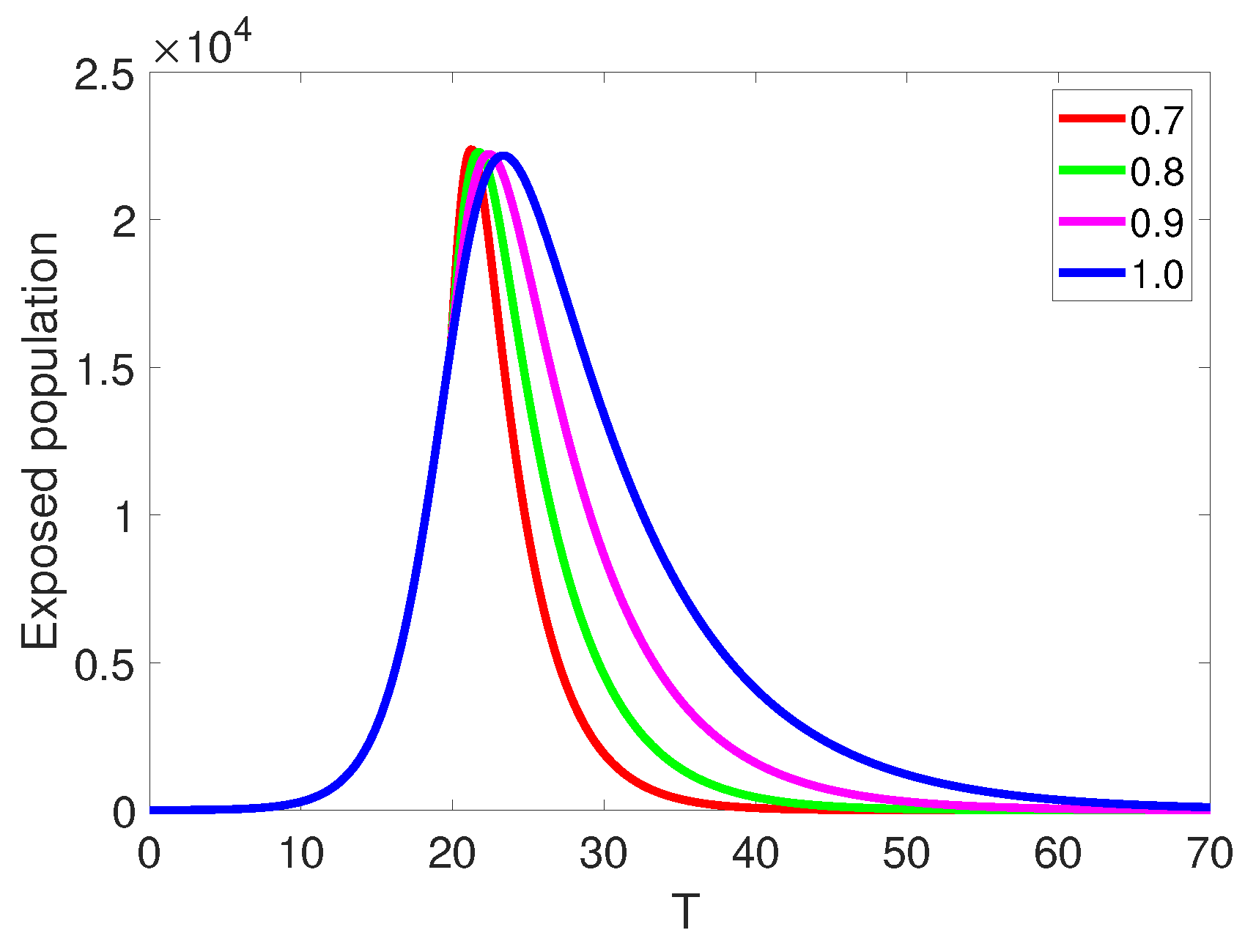
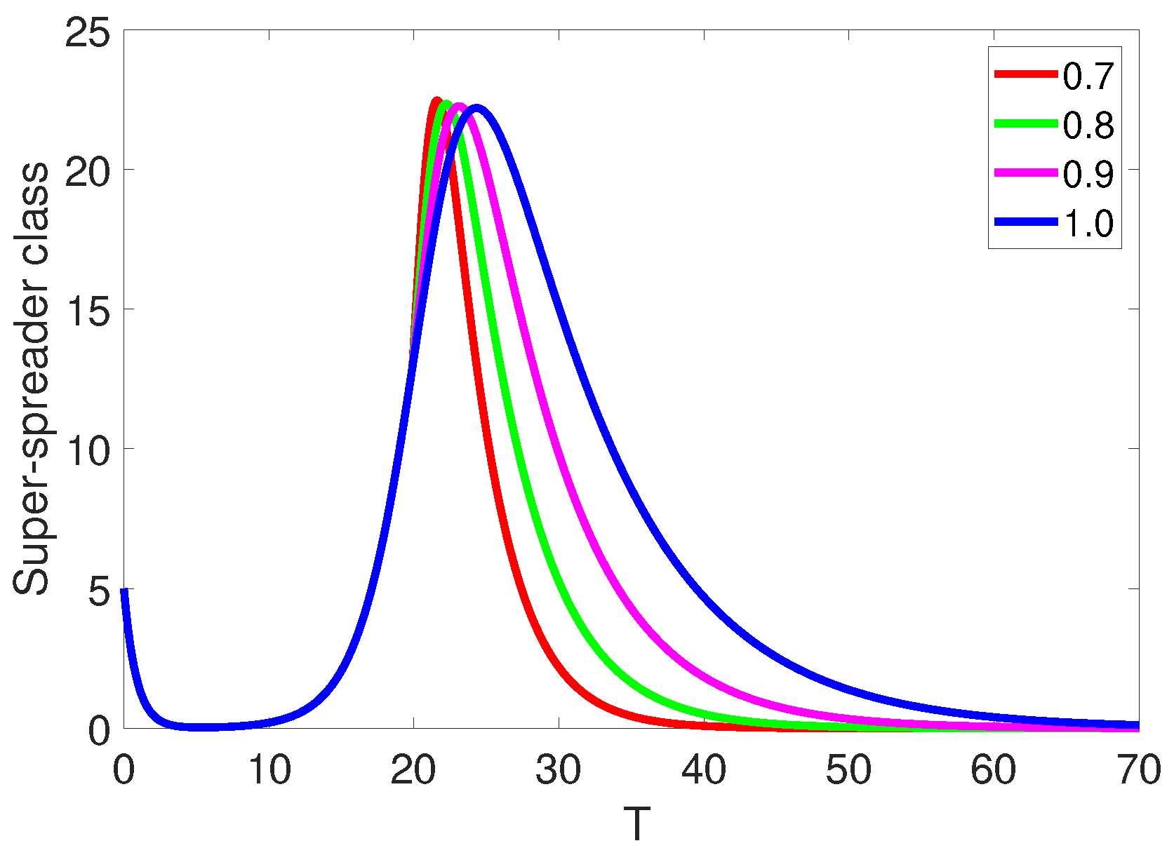
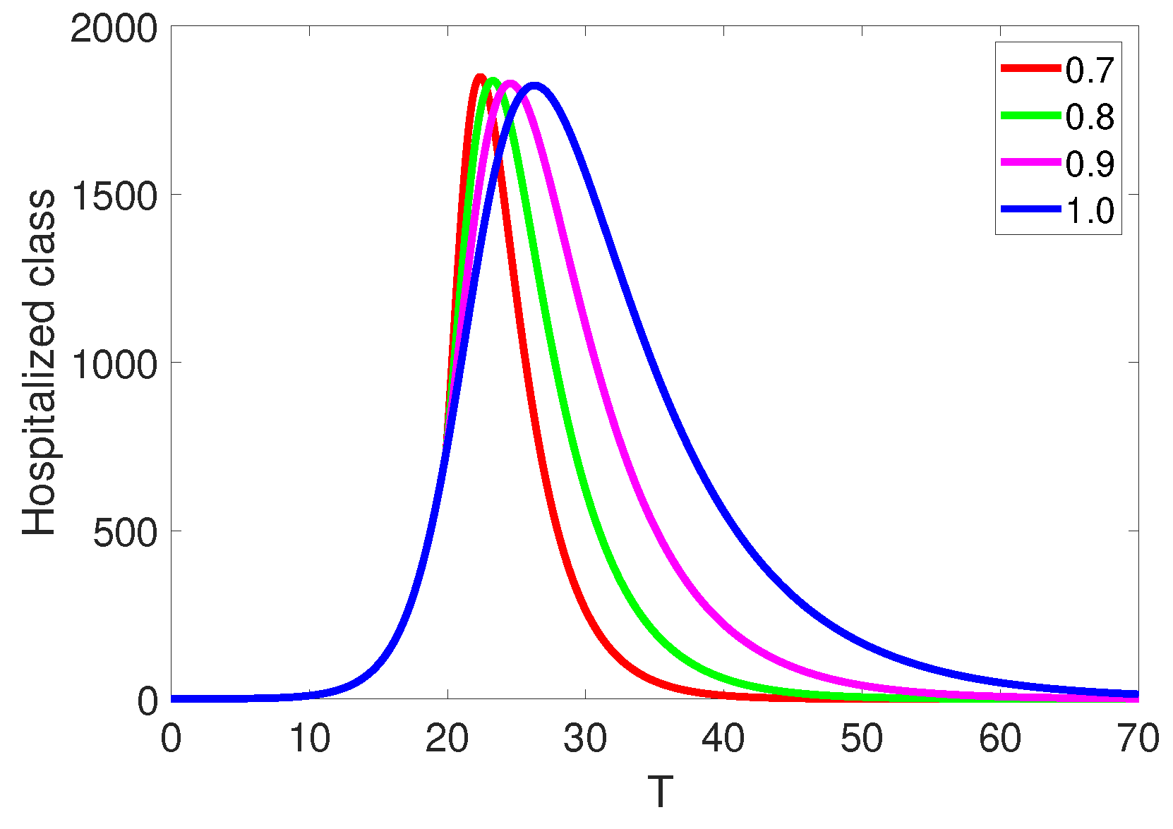
This section presents the simulations of the proposed PW model (2). In simulations of the approximate numerical findings, we have used the parameters as expressed in

Table 1. Parameter description and values of the suggested model [22].

Parameter	Definition	Value	Units
$\mu$	“spread from the diseased populace”	2.54	per day
l	“Transmissibility (relative) of $\mathrm{H}$”	1.56	dimensionless
${\mu }^{\prime }$	“spread due to $\mathrm{P}$”	7.5	per day
${\kappa }^{{}^{\prime }}$	“Rate of exposed becoming infectious”	0.26	per day
${\sigma }_1$	“Rate of exposed individuals becoming infectious I”	0.579	dimensionless
${\sigma }_2$	“Rate of the exposed becoming super-spreaders”	0.099	dimensionless
${\alpha }_a$	“Rate at which individuals hospitalized”	0.93	per day
${\alpha }_i$	“Rate recovery with no hospitalization”	0.269	per day
${\alpha }_r$	“Recovered hospitalized patients’ rate”	0.5	per day
${\omega }_i$	“Rate of deaths due to infections”	3.49	per day
${\omega }_p$	“Disease influenced rate of deaths due to $\mathrm{P}$”	1.00001	per day
${\omega }_h$	“Disease influenced rate of deaths due to hospitalized”	0.30001	per day

. The initial values are used as $\left[\mathcal{S}\right(0),\mathcal{E}(0),\mathcal{I}(0),\mathcal{P}(0),\mathcal{A}(0),\mathcal{H}(0),\mathcal{R}(0),\mathcal{F}(0),]=[43993,1,1,5,0,0,0,0]$. To simulate the obtained results with classical and fractional operators, we make a partition of interval $[0,T]$ to two other intervals, which are $(0,t_1]=(0,35]$ and $[t_1,T]=[35,200]$. We consider the classical derivative in the interval $(0,t_1]$ and in the second one, the Caputo operator is used. Thus, the first interval projects the behavior of the PW COVID-19 system (2) in the sense of a classical operator, and dynamics in the second part of the interval show the evolution of the considered system with a variety of FOs in Caputo’s sense. In Figure 1, Figure 2, Figure 3, Figure 4, Figure 5, Figure 6, Figure 7 and Figure 8, the value of $\delta$ is used as $(blue,1.00)$, $(red,0.9)$, $(green,0.8)$, and $(red,0.7)$.

Figure 1 depicts the behavior of susceptible people. Figure 2 and Figure 3 present the evolution of that of exposed and infected individuals, respectively.

In the same way, Figure 4 and Figure 5 are simulated to perceive the behavior of $\mathcal{P}$ and $\mathcal{A}$, respectively. Moreover, Figure 6 depicts the behavior of the hospitalized population. Apart from this, Figure 7 and Figure 8 demonstrate the effects of the piecewise operator on the dynamics of the recovered and dead populations, respectively. In Figure 1, one can observe that as time passes, the susceptible $\mathcal{S}$ decreases and a more rapid decrease can be observed when moved to a second subinterval, where the Caputo derivative is utilized with various fractional orders. Similarly, in Figure 2, the exposed populace $\mathcal{E}$ grows and then progressively decreases, demonstrating the crossover behavior at $t=t_1$ and becoming stable at $t=35$ at fractional order $0.7$. In Figure 3, the infected $\mathcal{I}$ approaches their maximal values at $t=25$, indicating a decline in the populace after $t=25$ and at small fractional order it becomes stable rapidly in the second subinterval.

In the same way, Figure 4 shows the behavior of superspreaders, which increases at the beginning and then declines with time to become stable faster at a lower fractional order. In Figure 5, the asymptomatic individual goes to the top value at $t=35$, then advances uniformly at fractional order $0.7$. Moreover, Figure 6 shows that there are a lot of hospitalized people at the beginning, which then decreases with time. In the same manner, Figure 7 and Figure 8 show that there are no recovered and dead individuals, respectively, at the start, which increases with time and then becomes stable.

Figure demonstrates the comparison between the simulated and real data of the three most affected countries in the world. For the simulation of Figure 9a,b, we have considered the parameter values as $\gamma =0.5$, ${\rho }_1=2.1$, and ${\rho }_2=0.09$, whereas the other values are as presented in Table 1. Here, the step size is used as $h=0.01$ and $\delta$ is supposed as $(blue,1.00)$, $(red,0.9)$, $(green,0.8)$, and $(cyan,0.7)$. Figure 9a presents the comparison between the infected populous vs. real data of the infected from India, whereas Figure 9b shows the comparison of the recovered individuals vs. real data of those who are recovered from COVID-19 in India. For the simulation of Figure 9c,d, we considered the parameter values as $\gamma =0.5$, ${\rho }_1=1.9$, and ${\rho }_2=0.03$, whereas the other values are as presented in Table 1. Here, the step size is used as $h=0.2$ and $\delta$ is supposed to be $(blue,1.00)$, $(red,0.95)$, $(green,0.90)$, and $(cyan,0.85)$. Figure 9c presents the comparison between the infected populous vs. real data of the infected from France, whereas Figure 9d shows the comparison of the recovered individuals vs. real data of those who are recovered from COVID-19 in France. Furthermore, for the simulation of Figure 9e,f, we considered the parameter values as $\gamma =0.8$, ${\rho }_1=2.9$ and ${\rho }_2=0.01$, whereas the other values are as presented in Table 1. Here, the step size is used as $h=0.2$ and $\delta$ is supposed as $(blue,1.00)$, $(red,0.9)$, $(green,0.7)$, and $(cyan,0.6)$. Figure 9c demonstrates the comparison between the infected individuals vs. real data of the infected from Italy, whereas Figure 9d shows the comparison of the recovered individuals vs. real data of those who are recovered from COVID-19 in Italy. From comparison, we observe that piecewise derivatives are very advantageous when compared to other classical and also fractional operators, because some of the data fit with the classical whereas some fit with different fractional order.

6. Conclusions

This paper examined the behavior of the COVID-19 model in the context of piecewise operators in the classical Caputo sense. We presented the existence–uniqueness of the solution with a piecewise derivative. To approximate the solution, we employed a piecewise numerical scheme utilizing Newton polynomials. Simulations were conducted for the considered model with different fractional orders. Additionally, a comparison between the simulated and real data from three different countries, namely India, France, and Italy, was presented, revealing the observation of the best-fitted dynamics. Furthermore, it was observed that piecewise operators offer significant advantages when compared to classical and fractional operators separately. It is worth noting that other fatal diseases exist in nature [30,31]. Some more advanced techniques such as bifurcations, control mechanisms, and neural networks [32,33,34,35,36,37] can be applied to study many epidemiological models. In our future research, we will investigate the cross-behavior of these models.

References

1. Fan, Y.; Zhao, K.; Shi, Z.-L.; Zhou, P. Bat Coronaviruses in China. Viruses 2019, 11, 210. [Google Scholar] [PubMed] [Green Version]
2. Wang, C.; Horby, P.W.; Hayden, F.G.; Gao, G.F. A novel coronavirus outbreak of global health concern. Lancet 2020, 395, 470–473. [Google Scholar] [PubMed] [Green Version]
3. Guo, Y.-R.; Cao, Q.-D.; Hong, Z.-S.; Tan, Y.-Y.; Chen, S.-D.; Jin, H.-J. The origin, transmission and clinical therapies on coronavirus disease 2019 (COVID-19) outbreak—An update on the status. Mil. Med. Res. 2020, 7, 11. [Google Scholar] [PubMed] [Green Version]
4. Riou, J.; Althaus, C.L. Pattern of early human-to-human transmission of Wuhan 2019 novel coronavirus (2019-nCoV), December 2019 to January 2020. Eurosurveillance 2020, 25, 2000058. [Google Scholar] [CrossRef] [PubMed] [Green Version]
5. Roser, M.; Ortiz-Ospina, E.; Ritchie, H.; Hasell, J. Coronavirus Pandemic (COVID-19). Our World in Data. 2020. Available online: https://ourworldindata.org/coronavirus (accessed on 1 January 2023).
6. World Health Organization (WHO). Available online: https://www.who.int/emergencies/diseases/novel-coronavirus-2019/technical-guidance2020 (accessed on 1 January 2023).
7. Kizito, M.; Tumwiine, J. A mathematical model of treatment and vaccination interventions of pneumococcal pneumonia infection dynamics. J. Appl. Math. 2018, 2018, 2539465. [Google Scholar] [CrossRef]
8. Pinto, C.M.A.; Machado, J.A.T.; Simón, C.B. Modified SIQR model for the COVID-19 outbreak in several countries. Math. Methods Appl. Sci. 2022. ahead of print. [Google Scholar] [CrossRef]
9. Kucharski, A.J.; Russell, T.W.; Diamond, C.; Liu, Y.; Edmunds, J.; Funk, S.; Eggo, R.M.; Sun, F.; Jit, M.; Munday, J.D.; et al. Early dynamics of transmission and control of COVID-19: A mathematical modelling study. Lancet Infect. Dis. 2020, 20, P553–P558. [Google Scholar] [CrossRef] [Green Version]
10. Fanelli, D.; Piazza, F. Analysis and forecast of COVID-19 spreading in China, Italy and France. Chaos Solitons Fractals 2020, 134, 109761. [Google Scholar]
11. Ullah, S.; Khan, M.A. Modeling the impact of non-pharmaceutical interventions on the dynamics of novel coronavirus with optimal control analysis with a case study. Chaos Solitons Fractals 2020, 139, 110075. [Google Scholar]
12. Alasmawi, H.; Aldarmaki, N.; Tridane, A. Modeling of a super-spreading event of the mers-corona virus during the hajj season using simulation of the existing data. Int. J. Statist. Med. Biolog. Res. 2017, 1, 24–30. [Google Scholar]
13. Kojabad, E.A.; Rezapour, S. Approximate solutions of a sum-type fractional integro-differential equation by using Chebyshev and Legendre polynomials. Adv. Differ. Equ. 2017, 2017, 351. [Google Scholar]
14. Hui, D.S.; Azhar, E.I.; Kim, Y.-J.; Memish, Z.A.; Oh, M.-D.; Zumla, A. Middle East respiratory syndrome coronavirus: Risk factors and determinants of primary, household, and nosocomial transmission. Lancet Infect. Dis. 2018, 18, 217–227. [Google Scholar]
15. Khan, M.A.; Atangana, A. Modeling the dynamics of novel coronavirus (2019-nCoV) with fractional derivative. Alex. Eng. J. 2020, 59, 2379–2389. [Google Scholar] [CrossRef]
16. Thabet, S.T.M.; Abdo, M.S.; Shah, K.; Abdeljawad, T. Study of transmission dynamics of COVID-19 mathematical model under ABC fractional order derivative. Results Phys. 2020, 19, 103507. [Google Scholar]
17. Shah, K.; Abdeljawad, T.; Mahariq, I.; Jarad, F. Qualitative analysis of a mathematical model in the time of COVID-19. Biomed Res. Int. 2020, 2020, 5098598. [Google Scholar]
18. Podlubny, I. An introduction to fractional derivatives, fractional differential equations, to methods of their solution and some of their applications. Math. Sci. Eng. 1999, 198, 340. [Google Scholar]
19. Podlubny, I. Fractional Differential Equations: An Introduction to Fractional Derivatives, Fractional Differential Equations, to Methods of Their Solution and Some of Their Applications; Elsevier: Amsterdam, The Netherlands, 1998. [Google Scholar]
20. Baleanu, D.; Jajarmi, A.; Bonyah, E.; Hajipour, M. New aspects of poor nutrition in the life cycle within the fractional calculus. Adv. Differ. Equ. 2018, 2018, 230. [Google Scholar]
21. Ahmad, S.; Ullah, A.; Al-Mdallal, Q.M.; Khan, H.; Shah, K.; Khan, A. Fractional order mathematical modeling of COVID-19 transmission. Chaos Solitons Fractals 2020, 139, 110256. [Google Scholar]
22. Ndaïrou, F.; Area, I.; Nieto, J.J.; Torres, D.F.M. Mathematical modeling of COVID-19 transmission dynamics with a case study of Wuhan. Chaos Solitons Fractals 2020, 27, 109846. [Google Scholar]
23. Atangana, A.; Araz, S.I. New concept in calculus: Piecewise differential and integral operators. Chaos Solitons Fractals 2021, 145, 110638. [Google Scholar]
24. Xu, C.; Alhejaili, W.; Saifullah, S.; Khan, A.; Khan, J.; El-Shorbagy, M.A. Analysis of Huanglongbing disease model with a novel fractional piecewise approach. Chaos Solitons Fractals 2022, 161, 112316. [Google Scholar]
25. Ansari, K.J.; Asma; Ilyas, F.; Shah, K.; Khan, A.; Abdeljawad, T. On new updated concept for delay differential equations with piecewise Caputo fractional-order derivative. Waves Random Complex Media 2023, 1–20. [Google Scholar] [CrossRef]
26. Saifullah, S.; Ahmad, S.; Jarad, F. Study on the dynamics of a piecewise tumor–immune interaction model. Fractals 2022, 30, 2240233. [Google Scholar]
27. Naowarat, S.; Ahmad, S.; Saifullah, S.; la Sen, M.D.; Akgül, A. Crossover Dynamics of Rotavirus Disease under Fractional Piecewise Derivative with Vaccination Effects: Simulations with Real Data from Thailand, West Africa, and the US. Symmetry 2022, 14, 2641. [Google Scholar]
28. Ahmad, S.; Yassen, M.F.; Alam, M.M.; Alkhati, S.; Jarad, F.; Riaz, M.B. A numerical study of dengue internal transmission model with fractional piecewise derivative. Results Phys. 2022, 39, 105798. [Google Scholar]
29. Abdelmohsen, S.A.M.; Yassen, M.F.; Ahmad, S.; Abdelbacki, A.M.M.; Khan, J. Theoretical and numerical study of the rumours spreading model in the framework of piecewise derivative. Eur. Phys. J. Plus 2022, 137, 738. [Google Scholar]
30. Chávez, J.P.; Wijaya, K.P.; Pinto, C.M.A.; Simón, C.B. A model for type I diabetes in an HIV-infected patient under highly active antiretroviral therapy. Chaos Solitons Fractals 2022, 155, 111716. [Google Scholar]
31. Pinto, C.M.A.; Carvalho, A.R.M. Analysis of a Non-integer Order Model for the Coinfection of HIV and HSV-2. Int. J. Nonlinear Sci. Numer. Simul. 2020, 21, 291–302. [Google Scholar] [CrossRef]
32. Xu, C.; Zhang, W.; Aouiti, C.; Liu, Z.; Yao, L. Bifurcation insight for a fractional-order stage-structured predator–prey system incorporating mixed time delays. Math. Methods Appl. Sci. 2023, 46, 9103–9118. [Google Scholar] [CrossRef]
33. Xu, C.; Mu, D.; Liu, Z.; Pang, Y.; Liao, M.; Aouiti, C. New insight into bifurcation of fractional-order 4D neural networks incorporating two different time delays. Commun. Nonlinear Sci. Numer. Simul. 2023, 118, 107043. [Google Scholar]
34. Ou, W.; Xu, C.; Cui, Q.; Liu, Z.; Pang, Y.; Farman, M.; Ahmad, S.; Zeb, A. Mathematical study on bifurcation dynamics and control mechanism of tri-neuron bidirectional associative memory neural networks including delay. Math. Methods Appl. Sci. 2023. [Google Scholar] [CrossRef]
35. Xu, C.; Mu, D.; Pan, Y.; Aouiti, C.; Yao, L. Exploring Bifurcation in a Fractional-Order Predator-Prey System with Mixed Delays. J. Appl. Anal. Comput. 2023, 13, 1119–1136. [Google Scholar]
36. Xu, C.; Mu, D.; Liu, Z.; Pang, Y.; Liao, M.; Li, P.; Yao, L.; Qin, Q. Comparative exploration on bifurcation behavior for integer-order and fractional-order delayed BAM neural networks. Nonlinear Anal. Model. Control. 2022, 27, 1030–1053. [Google Scholar] [CrossRef]
37. Xu, C.J.; Mu, D.; Liu, Z.X.; Pang, Y.C.; Liao, M.X.; Li, P. Bifurcation dynamics and control mechanism of a fractional-order delayed Brusselator chemical reaction model. Match Commun. Math. Comput. Chem. 2023, 89, 73–106. [Google Scholar]
Figure 1. The behavior of susceptibles in the system (2) with t 1 = 20 .
Fractalfract 07 00501 g001
Figure 2. The behavior of exposed population of model (2) with t 1 = 20 .
Fractalfract 07 00501 g002
Figure 3. The behavior of those who are infected in the system (2) with t 1 = 20 .
Fractalfract 07 00501 g003
Figure 4. The behavior of superspreader populous of model (2) with t 1 = 20 .
Fractalfract 07 00501 g004
Figure 5. The dynamics of asymptomatic population in model (2) with t 1 = 20 .
Fractalfract 07 00501 g005
Figure 6. The dynamics of hospitalized people of model (2) with t 1 = 20 .
Fractalfract 07 00501 g006
Figure 7. The dynamics of recovered class of model (2) with t 1 = 20 .
Fractalfract 07 00501 g007
Figure 8. The dynamics of fatality class of model (2) with t 1 = 20 .
Fractalfract 07 00501 g008
Figure 9. Comparison between simulated and real data of the infected and recovered population in three different countries of model (2).
Fractalfract 07 00501 g009aFractalfract 07 00501 g009b