Fractional Gradient Optimizers for PyTorch: Enhancing GAN and BERT

Abstract

Machine learning is a branch of artificial intelligence that dates back more than 50 years. It is currently experiencing a boom in research and technological development. With the rise of machine learning, the need to propose improved optimizers has become more acute, leading to the search for new gradient-based optimizers. In this paper, the ancient concept of fractional derivatives has been applied to some optimizers available in PyTorch. A comparative study is presented to show how the fractional versions of gradient optimizers could improve their performance on generative adversarial networks (GAN) and natural language applications with Bidirectional Encoder Representations from Transformers (BERT). The results are encouraging for both state-of-the art algorithms, GAN and BERT, and open up the possibility of exploring further applications of fractional calculus in machine learning.

1. Introduction

Several machine learning techniques are posed as optimization problems and owe their success to gradient-based methods. The success is twofold: first, the optimization task itself, and second, the widespread adoption by the AI community. For example, in machine learning and specifically in neural networks, the multilayer perceptron learning technique defines a training error surface that depends on synaptic weights as free parameters that can be optimized with the backpropagation algorithm, which is a gradient-descent-based algorithm. It finds the optimal parameters to minimize the training error. The success lies not only in solving the optimization problem by minimizing the training error but also in maximizing the generalization capacity on a test dataset, avoiding overfitting, which has led to wide use of multilayer perceptrons in various applications by the artificial intelligence community [1].

Recently, with the boom in research and technological development of machine learning, the need to propose improved optimizers has become more acute, leading to the search for new gradient-based optimizers. In this respect, the authors of [2] performed a comparison of 15 optimizers chosen from a large list of 144 optimizers and schedulers, showing the variability of techniques that continues to evolve and grow. Of course, they include the fundamental SGD and Adam optimizers. The former because it is the cornerstone of all gradient-based techniques [3], whereas the latter calculates adaptive learning rates and is considered state of the art in deep learning [4].

Additionally, a survey of optimization algorithms for neural networks is presented in [5], where modifications to basic optimization algorithms are studied. The paper [6] presents the latest contributions for deep learning based on stochastic gradient-descent methods and a summary of applications of network architectures together with the methods used for specific purposes.

A brief summary of relevant variants of SGD, Adam, Adagrad, and Adadelta is also presented in [7], along with a review of their parameter-update formulas that reveals the combination of concepts, including momentum, velocity, learning rate adaptation, parameter normalization, and gradient-memory.

Although the majority of optimizers consider these concepts to enhance the training and the capacity of generalization, in this work, the ancient but powerful concept of fractional derivatives is applied to several gradient-based optimizers available in PyTorch [8,9]. In this way, several fractional versions of optimizers have been implemented for PyTorch, and they are presented as generalizations to the first-order derivative. In other words, the fractional derivative of $\nu$-order ($\nu \in {\mathbb{R}}^{+}$ ) includes the classical first-order gradient when $\nu =1$. From this point of view, it provides an additional freedom degree to the hyperparameters that allows us to exploit the properties and advantages of fractional derivatives, including the effect of non-locality which obtains information from the neighborhood of the derivation-point by applying integro-differential operators [10,11].

Certainly, the application of fractional derivatives is not recent, and it can be verified in previous works on different areas, including linear viscoelastivity [12], partial differential equations [13], signal processing [14], and image processing [15], among others.

With respect to neural networks, there is also evidence of applications of fractional derivatives. For example, in [16], Fractional Physics-Informed Neural Networks are developed employing partial differential equations embedded in architectures of feedforward neural networks with automatic differentiation to optimize the network parameters. Another work is [17] on the study of two-layer neural networks trained with backpropagation and fractional derivatives. The authors of [18] studied a fractional deep backpropagation algorithm for neural networks with $L_2$-regularization, and in [19] the stability for Hopfield neural networks of fractional order is investigated, just to mention a few works but the list of fractional-gradient applications seems to grow promisingly.

Although there are many works that use fractional-order derivatives in neural networks, it is notorious that they focus on ad hoc solutions and do not offer easy adaptation or reusability to other applications. Thereupon, it has been identified the need and importance of implementing fractional optimizers in frameworks such as PyTorch [9] that offer versatility and flexibility to apply gradient-based optimizers to different areas of great interest to the machine learning community.

In this regard, about frameworks for machine learning, a related work is [7] that presents a Keras–Tensorflow [20,21] implementation of several fractional optimizers successfully applied to human activity recognition.

Since these frameworks have become a popular and powerful tool that takes advantage of high-performance computing using GPUs and cloud platforms, this article aims to contribute to the implementation of fractional optimizers by extending current versions of integer-order gradient algorithms available in PyTorch. Once described how the implementation of fractional optimizers is done, two case studies are presented, firstly on generative adversarial networks (GAN) [22] and secondly on natural language processing (NLP) with Bidirectional Encoder Representations from Transformers (BERT) [23]. Many other applications may be possible, but for now, only these are shown. The results are encouraging and are expected to provide enough motivation and justification for the success of applying fractional calculus concepts in machine learning.

The remainder of the paper has the following structure. In Section 2, fundamental concepts are revised of fractional derivatives to propose a gradient-update formula based on the Caputo definition. In Section 3, fractional implementations for PyTorch are presented with some comparative experiments that aim to show how the fractional versions of gradient-based optimizers could improve their performance on GAN and NLP applications with BERT. Finally, Section 4 presents some discussions following the experiments and comments on some directions for future work.

2. Materials

The following topics are covered in this section: the Caputo fractional derivative, the backpropagation update formula for multilayer perceptrons (MLP) and the implementations of fractional gradient optimizers for PyTorch. It provides the necessary materials to develop the experiments that support the conclusions.

2.1. Caputo Fractional Derivative

Definition 1.

Let $a,x\in \mathbb{R}$, $\nu >0$ and  $n=[\nu +1]$. The Caputo fractional derivative of order ν for $f\left(x\right)$ is  [17]:

$${}_a^C{D}_x^{\nu }f\left(x\right)=\frac{1}{\mathsf{\Gamma }(n-\nu )}{\int }_a^x{(x-y)}^{n-\nu -1}{f}^{\left(n\right)}\left(y\right)dy.$$

(1)

It is one of the most preferred definitions of fractional derivative, since if $f\left(x\right)=C$, $C\in \mathbb{R}$, then ${}_a^C{D}_x^{\nu }f\left(x\right)=0$ [18]. In particular, for $\nu =1$ it corresponds to the classical differential calculus, that means that the derivative of a constant is zero. In general, it is not the same for other definitions such as the Riemman–Liouville or Grünwald–Letnikov [17].

In Equation (1), a convolutional kernel ${(x-y)}^{n-\nu -1}$ is used and for $f\left(x\right)=x^q$ it yields to [24]:

$$D_x^{\nu }{x}^q=\frac{\mathsf{\Gamma }(q+1)x^{q-v}}{\mathsf{\Gamma }(q-v+1)}.$$

(2)

Equation (2) represents a relevant property since it allows to extend the integer-order gradient optimizers to their fractional versions, as described in Section 2.2.

2.2. Backpropagation Update Formula for MLP

Given the original backpropagation formula to update the parameters of MLP, the corresponding fractional versions will be obtained.

Let a training set ${\{X^i,O^i\}}_{i=1}^N$ with N samples, and a neural network architecture described as follows:

• X is the input layer (input data),
• H hidden layers,
• O is the output layer,
• L layers, $L=H+1$ because of the hidden layers and the output layer,
• $w_{kj}^l$ is a matrix of synaptic weights, $l\in [1,L-1]$, that connects neuron k of layer $l+1$ with neuron j of layer l,
• $w_{kj}^0$ are synaptic weights ($l=0$) that connect the first hidden layer with X,
• $o_{ki}$ is the desired output of neuron k at output layer when the i-th input data is presented,
• $\phi \left(x\right)$ is the activation function in the L layers,
• $a_{ki}^L$ is the output of neuron k at output layer O, when the i-th input data is presented and $a_k^L=\phi \left(p_k^L\right)$ at layer O,
• $p_k^l=\sum w_{kj}^l·a_j^{l-1}$ is the potential activation of neuron k at layer l, $1\le l\le L$, with inputs $a_j^{l-1}$. For $l-1=0$, $a_j^0=X_j$ considering the j-th component of X,
• $a_k^l=\phi \left(p_k^l\right)$ is the output of neuron k at a hidden layer l, $1\le l<L$.

Note that, at the output layer, the error of neuron k is $e_{ki}=a_{ki}^L-o_{ki}$. Subindex i means that the i-th input pattern is presented to the neural network. For all the $n^L$ neurons, the error $E_i$ at the output layer is:

$$E_i=\frac{1}{2}\sum _{k=1}^{n^L}{e}_{ki}^2=\frac{1}{2}\sum _{k=1}^{n^L}{(a_{ki}^L-o_{ki})}^2$$

(3)

and the cumulative error of the N training samples is E:

$$E=\sum _{i=1}^N{E}_i=\frac{1}{2}\sum _{i=1}^N\sum _{k=1}^{n^L}{(a_{ki}^L-o_{ki})}^2.$$

(4)

The main goal of the backpropagation algorithm is to find optimal values of the free parameters of the weight matrix that minimize E.

In the backpropagation algorithm, the error of the output layer O is propagated to the hidden layers in reverse order until it reaches the input layer, and the gradient-descent updates are applied to each layer.

The optimization with the gradient-descent method applied to the weight updates $\Delta w_{kj}^l$ is:

$$\Delta w_{kj}^l=-\eta \frac{\partial E_i}{\partial w_{kj}^l}=-\eta D_{w_{kj}^l}{E}_i$$

(5)

that points to the direction where $E_i$ decays. Here, $\eta >0$ is the learning rate.

It should be clarified that Equation (5) uses the nomenclature $D_{w_{kj}^l}{E}_i$ to match with the Caputo fractional derivative definition of Section 2.1.

At this point, the local gradient is defined as:

$${\delta }_k^l=\frac{\partial E_i}{\partial p_k^l}$$

(6)

and since

$$\frac{\partial E_i}{\partial w_{kj}^l}=\frac{\partial E_i}{\partial p_k^l}·\frac{\partial p_k^l}{\partial w_{kj}^l}=\frac{\partial E_i}{\partial p_k^l}·a_j^{l-1}={\delta }_k^l{a}_j^{l-1}$$

(7)

then, $\Delta w_{kj}^l$ can be expressed as:

$$\Delta w_{kj}^l=-\eta ·{\delta }_k^l·a_j^{l-1}.$$

(8)

For $l=L$, Equation (6) becomes ${\delta }_k^L$ and then, at the output layer O:

$${\delta }_k^L=e_{ki}·{\phi }^{\prime }\left(p_k^L\right).$$

(9)

For $1\le l<L$, the local gradient for hidden layers is:

$${\delta }_j^l={\phi }^{\prime }\left(p_j^l\right)·\sum _{k=1}^{n^{l+1}}{\delta }_k^{l+1}·w_{kj}^{l+1}$$

(10)

and consequently, the weight updates are:

$$\Delta w_{kj}^l=-\eta {\delta }_k^l{a}_j^{l-1}.$$

(11)

The Formulas (3) to (11) are well known by the neural network community. However, now, to make way for the fractional optimizers, the same approach for the first-order derivative $D_{w_{kj}^l}{E}_i$ can be used with the fractional gradient $D_{w_{kj}^l}^{\nu }{E}_i$. In such case, the chain rule yields to [18]:

$$D_{w_{kj}^l}^{\nu }{E}_i=\frac{\partial E_i}{\partial w_{kj}^l}·D_{w_{kj}^l}^{\nu }{w}_{kj}^l={\delta }_k^l·a_j^{l-1}·\frac{{\left(w_{kj}^l\right)}^{1-\nu }}{\mathsf{\Gamma }(2-\nu )}.$$

(12)

Equation (12) seems identical to Equation (7) except by $\frac{{\left(w_{kj}^l\right)}^{1-\nu }}{\mathsf{\Gamma }(2-\nu )}$ that is obtained when Equation (2) is applied to $w_{kj}^l$. Note that if $\nu =1$, Equation (12) becomes the classical integer case. So, Equation (12) represents a gradient-descent generalization, for $\nu >0$.

In practice, it is necessary to avoid two conditions:

• When synaptic weights take zero values that yields to the indetermination of $\frac{{\left(w_{kj}^l\right)}^{1-\nu }}{\mathsf{\Gamma }(2-\nu )}$ for $1-\nu <0$,
• When $1-\nu$ is rational, let $1-\nu =\frac{r}{s}$ and s is even (for example $r=1$ and $s=2$) hence if $w_{kj}^l<0$, then complex values will be generated.

These situations have been explored previously in [7] and a solution consists of replacing $w_{kj}^l$ by $\left|w_{kj}^l\right|+ϵ$, for $ϵ>0$. In this way, the fractional gradient factor $f_w^{\nu }$ is defined as:

$$f_w^{\nu }:=\frac{\left(\right|w_{kj}^l{|+ϵ)}^{1-\nu }}{\mathsf{\Gamma }(2-\nu )}$$

(13)

and the limit exists, and is equal to 1, for $f_w^{\nu }$ as $\nu \to 1$.

Hence, Equation (12) becomes:

$$D_{w_{kj}^l}^{\nu }{E}_i={\delta }_k^l·a_j^{l-1}·f_w^{\nu }={\delta }_k^l·a_j^{l-1}·\frac{\left(\right|w_{kj}^l{|+ϵ)}^{1-\nu }}{\mathsf{\Gamma }(2-\nu )}$$

(14)

that generalizes the known gradient-descent update rule.

It is worth noting that $f_w^{\nu }$ is not negative for $\nu <2$. Therefore, the fractional gradient of Equation (14) modifies the magnitude of the classical gradient $D_{w_{kj}^l}{E}_i$, but preserves the negative sign of the gradient-descent of Equation (5). Hence, the fractional gradient also points to the same direction of the gradient-descent on the error surface given by $E_i$ of Equation (3), and thus to the direction in which a loss function for the neural network will decay.

2.3. Fractional Gradient Optimizers for PyTorch

PyTorch is a Python-based scientific computing package for machine learning. As framework, PyTorch follows two purposes: (i) To use GPUs (ii) To provide automatic differentiation for neural networks [9].

The package torch.optim [8] implements various optimization algorithms such as SGD [3], Adam [4], Adadelta [25], Adagrad [26], AdamW [27] and RMSProp [28] among others.

To apply an optimizer in PyTorch is enough to use a line of code like the following for the SGD optimizer:

• opt=optim .SGD(model . parameters () , learning_rate=0.001 ,momentum=0.9)
• whereas the Adam optimizer can be used as follows:
• opt=optim .Adam(model . parameters () , learning_rate =0.001).

Now, since the main idea is to apply Equation (14) to obtain fractional gradient optimizers in PyTorch, simply multiply $f_w^{\nu }$ by the integer-gradient. For this purpose, a new class is defined in PyTorch with the prefix “F” for each existing optimizer. In the case of SGD, the new class is FGSD and the line

• __all__ = [ ’SGD’ , ’sgd’ ]

is replaced by

• __all__ = [ ’FSGD’ , ’fsgd’ ].

Moreover, the source code of the update method _single_tensor_sgd is modified as follows, in the Listing 1:

Listing 1. FSGD class definition and single_tensor_sgd method modification.

# Parameters: Set v= Cnnu.nnu, 0 < v < 2.0

Cnnu.nnu = 1.75

eps = 0.000001

class FSGD(Optimizer):

…

def _single_tensor_sgd (…):

…

for i, param in enumerate (params):

d_p = d_p_list [ i ] if not maximize else -d_p_list [ i ]

v = Cnnu.nnu

t1 = torch . pow( abs(d_p)+eps, 1-v )

t2 = torch . exp(torch . lgamma(torch . tensor(2.0-v)))

d_p = d_p * t1/ t2

Listing 1. FSGD class definition and single_tensor_sgd method modification.

# Parameters: Set v= Cnnu.nnu, 0 < v < 2.0

Cnnu.nnu = 1.75

eps = 0.000001

class FSGD(Optimizer):

…

def _single_tensor_sgd (…):

…

for i, param in enumerate (params):

d_p = d_p_list [ i ] if not maximize else -d_p_list [ i ]

v = Cnnu.nnu

t1 = torch . pow( abs(d_p)+eps, 1-v )

t2 = torch . exp(torch . lgamma(torch . tensor(2.0-v)))

d_p = d_p * t1/ t2

The same procedure can be applied to other gradient-descent optimizers. Let us consider another example with Adam.

The new fractional optimizer is FAdam, and it was obtained by modifying the _single_tensor_adam method of the class FAdam, as described below in the Listing 2:

Listing 2. FAdam class definition and single_tensor_adam method modification.

#Parameters: Set v= Cnnu.nnu, 0 < v < 2.0

Cnnu.nnu = 1.75

eps = 0.000001

class FAdam(Optimizer):

…

def _single_tensor_adam (…):

…

for i , param in enumerate (params):

grad = grads [ i ] if not maximize else -grads [ i ]

v = Cnnu . nnu

t1=torch . pow( abs(grad)+eps , 1-v )

t2=torch . exp ( torch.lgamma(torch . tensor(2.0-v)))

grad = grad * t1/t2

Listing 2. FAdam class definition and single_tensor_adam method modification.

#Parameters: Set v= Cnnu.nnu, 0 < v < 2.0

Cnnu.nnu = 1.75

eps = 0.000001

class FAdam(Optimizer):

…

def _single_tensor_adam (…):

…

for i , param in enumerate (params):

grad = grads [ i ] if not maximize else -grads [ i ]

v = Cnnu . nnu

t1=torch . pow( abs(grad)+eps , 1-v )

t2=torch . exp ( torch.lgamma(torch . tensor(2.0-v)))

grad = grad * t1/t2

For the purposes of this paper, the fractional versions of AdamW, RMSProp, and Adadelta optimizers were also implemented. However, the same methodology can be applied to other optimizers.

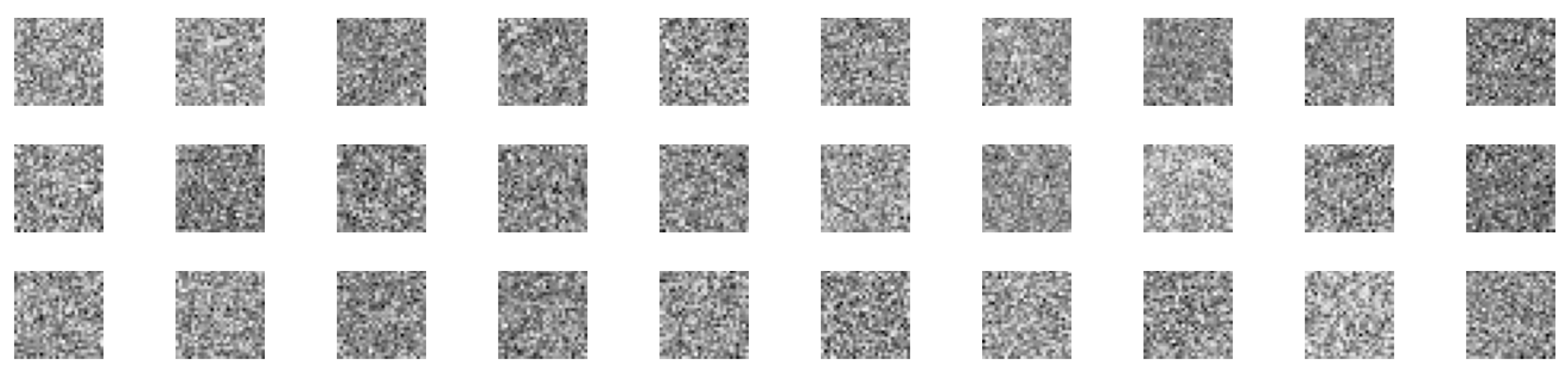
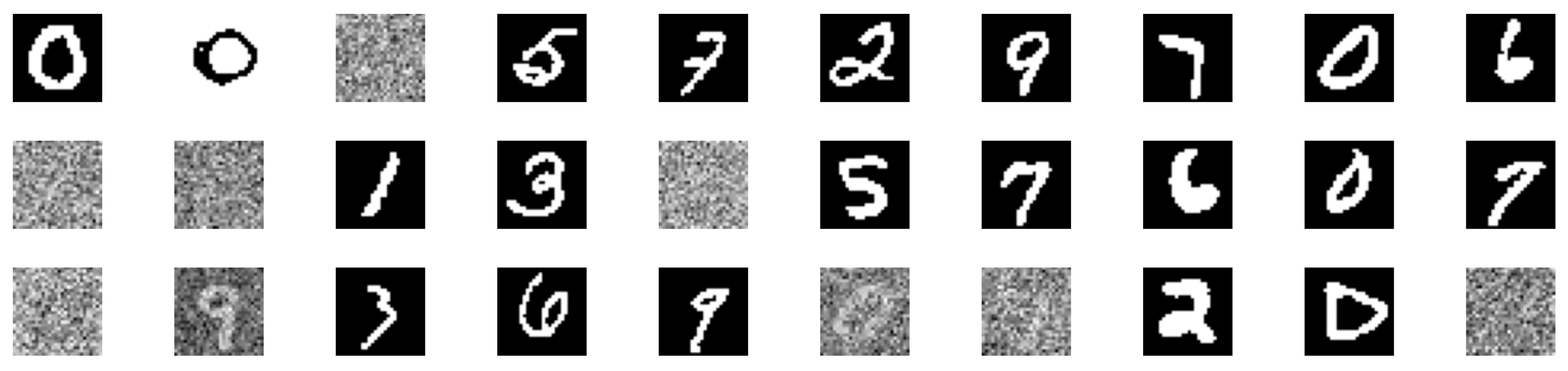
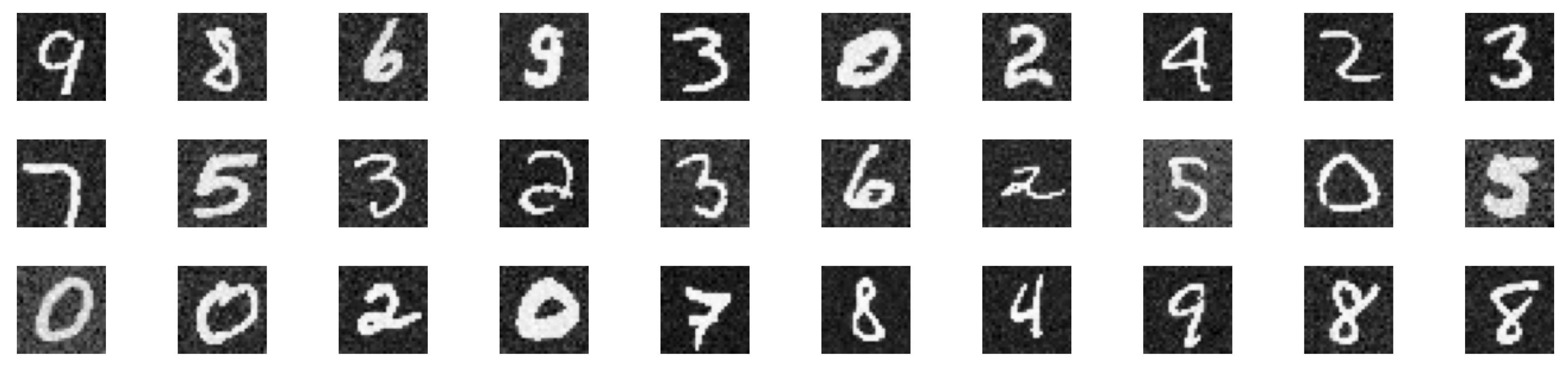
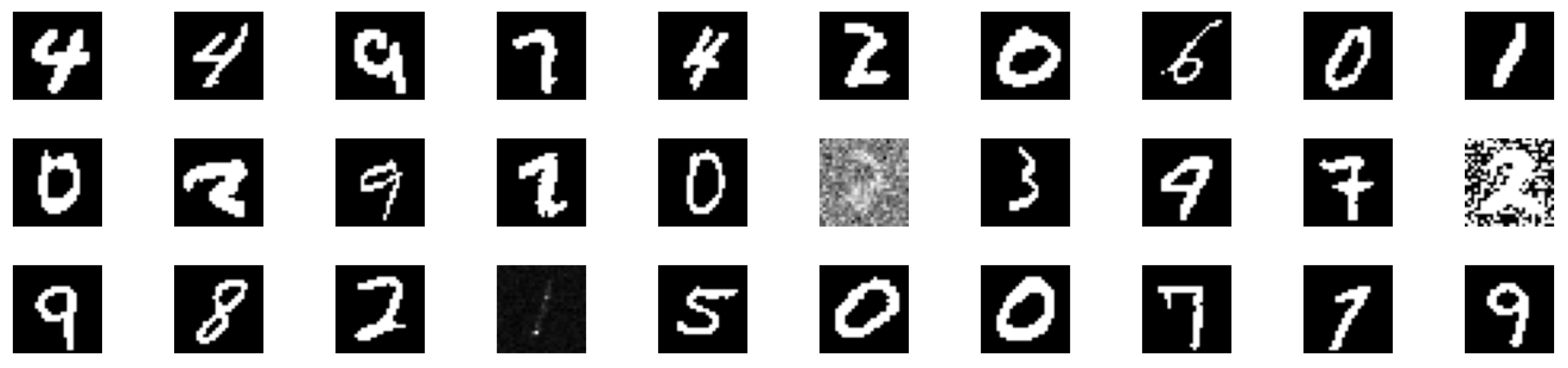
2.4. Fractional GAN

Generative Adversarial Networks (GAN) constitute a representative case of artificial creativity where two artificial neural networks are confronted: the generative G that proposes instances and the discriminative D that tries to detect the degree of falsehood of those instances. After repeating the algorithm, the result is a set of objects that share many characteristics of the training objects but are not identical to them.

If G and D use MLP, then backpropagation can be used to train the whole system [22]. In this way, the generative and discriminative models can apply gradient-descent optimizers, and consequently is possible to create fractional versions of G and D. Thus, a Fractional Generative Adversarial Network (FGAN) is obtained.

In connection with the above, the proposed FGAN minibatch stochastic gradient-descent training algorithm is the one shown in Algorithm 1, which is based on the integer gradient version for GAN-training described in [22]. Essentially, both stochastic gradients for the generator $g_{{\theta }_g}$ and discriminator $g_{{\theta }_d}$ are updated with the fractional factor $f_{{\theta }_d}^{\nu }$ and $f_{{\theta }_g}^{\nu }$ respectively (see lines 5 and 8 of Algorithm 1). In this sense, the FGAN represents a generalization of the GAN version.

Algorithm 1 Fractional GAN minibatch stochastic gradient-descent training algorithm.

1: for number of training iterations do 2:    for k steps do 3:       Sample minibatch of m noise samples {z(1), … , z(m)} from noise prior $p_g\left(z\right)$. 4:       Sample minibatch of m examples {x(1), … , x(m)} from data generating distribution $p_{data}\left(x\right)$. 5:       Update the discriminator by ascending its $\mathbf{fractional}$ stochastic gradient:     $g_{{\theta }_d}={\nabla }_{{\theta }_d}\frac{1}{m}{\sum }_{i=1}^m[logD\left(x^{\left(i\right)}\right)+log(1-D\left(G\left(z^{\left(i\right)}\right)\right))]$     $f_{{\theta }_d}^{\nu }=\frac{\left(\right|{\theta }_d^l{|+ϵ)}^{1-\nu }}{\mathsf{\Gamma }(2-\nu )}$     $g_{{\theta }_d}^{\nu }=g_{{\theta }_d}*f_{{\theta }_d}^{\nu }$ 6:    end for 7:    Sample minibatch of m noise samples {z(1), …, z(m)} from noise prior $p_g\left(z\right)$. 8:    Update the generator by descending its $\mathbf{fractional}$ stochastic gradient:    $g_{{\theta }_g}={\nabla }_{{\theta }_g}\frac{1}{m}{\sum }_{i=1}^{m}log(1-D\left(G\left(z^{\left(i\right)}\right)\right))$     $f_{{\theta }_g}^{\nu }=\frac{\left(\right|{\theta }_g^l{|+ϵ)}^{1-\nu }}{\mathsf{\Gamma }(2-\nu )}$     $g_{{\theta }_g}^{\nu }=g_{{\theta }_g}*f_{{\theta }_g}^{\nu }$ 9: end for     The gradient-based updates can use any $\mathbf{fractional}$ gradient-based learning rule

2.5. Fractional BERT

BERT is the acronym of Bidirectional Encoder Representations from Transformers and is a machine learning and language representation model that involves the transformer architecture with encoder and decoder modules to extract patterns or representations from data [23]. BERT was developed in the context of computational linguistic and uses bidirectional transformers to learn from both the left and right contexts of a vocabulary. BERT combines two complementary tasks: Pre-training and Fine-tuning. Pre-training uses a lot of unlabeled data to train the model. Fine-tuning is a transfer-learn step where the previous learning is potentiated on specific labeled data for different applications.

The encoder, conformed by a self-attention layer and a feed-forward neural network, aims to map words to intermediate representations together with their relationships.

The decoder has the same structure as the encoder, but inserts a middle layer of Encoder-Decoder Attention.

The main goal is to model patterns of long sequences to improve some drawbacks of previous approaches, such as LSTM [29] that only models a single context direction.

Since BERT includes neural network modules, and they are frequently optimized via gradient methods, fractional gradient optimizers can be applied to obtain a Fractional BERT version (FBERT). Essentially, the unique difference is the use of fractional optimizers, described in Section 2.3, instead of others based on integer-order derivatives.

The fractional optimizers of this paper have been included in a torch.Foptim package that refers to Fractional Optimization for PyTorch. Then, instead of using a PyTorch optimizer such as Adam from the package torch.optim with a line of code like this

• optim = optim.Adam(model.parameters(), learning_rate=0.001)
• a fractional optimizer from the package torch.Foptim can be used. In case of the fractional Adam (FAdam) the code is as follows:
• optim = Foptim.FAdam(model.parameters(), learning_rate=0.001).

It is emphasized that for $\nu =1.0$, the fractional case is reduced to the well-known integer case.

3. Results

In this section, two experiments are described, and their results are shown.

3.1. Experiment 1: FGAN

A first experiment implements an FGAN based on [30] that presents a GAN trained with the MNIST [31] dataset of grayscale images of 28 × 28 pixels. The discriminator network D considers both real and fake images as unidimensional 1 × 784 vectors. The cost function is:

$$D_{cost}=-log(D_{l2rA)}+log(1.0-D_{l2fA})$$

(15)

where $D_{l2rA}$ is the output of D with real images as inputs, and $D_{l2fA}$ corresponds to the output of D with fake images as inputs.

The FGAN was executed 30 times with FSGD and FAdam for different values of $\nu \in (0,2)$. Figure 1 and Figure 2 allow us to compare FSGD and FAdam with $\nu =1.0$. In other words, it represents the integer case of GAN+SGD vs. GAN+Adam (here + means “optimized with”). Note that in Figure 1, GAN+SGD fails completely since it does not produce any digit shape, whereas in Figure 2 GAN+Adam is better since it produces 22 of 30 digit images successfully.

Other experiments were developed with $\nu \in (0,2)$, but for reasons of space, only a few of them are reported. From these experiments, it was observed that FGAN + FSGD with $\nu =1.9$ gave the best results because it produced a digit shape in all the 30 executions, as illustrated in Figure 3.

In an attempt to obtain a similar result with FAdam, the FGAN was trained with some values of $\nu \in (0,2)$. The results for $\nu =0.1,0.3,0.7,0.9$ and $1.9$ are reported in Figure 4, Figure 5, Figure 6, Figure 7 and Figure 8, respectively. From these figures, it can be deduced that as $\nu$ grows, there is a greater number of failures because more images look noisy (no shape of some digit is visible), and the best of FGAN+FAdam was for $\nu =0.1$ with 3 fails, as shown in Figure 4.

Experimentally, it was not possible to find a $\nu$-value for FGAN+FAdam that always produced digits like FSGD. This suggests that SGD is still competitive in certain applications, such as GANs, by introducing the fractional gradient.

3.2. Experiment 2: FBERT

The second experiment is based on [32] that implements a BERT architecture in PyTorch and has 4 modules: Preprocessing, Building model, Loss and Optimization, and Training.

Preprocessing section. Defines a text data and applies several tasks, including those where the sentences are converted to lowercase and a vocabulary is created, as well as others where special tokens are defined as follows:

• hCLS: token classification,
• SEP: sentence separation,
• END: end of sentence,
• PAD: equal length and sentence truncation,
• MASK: mask creation and word replacement.

Additionally, embedding and masking tasks are included, and they are briefly described below.

Embedding tasks. Three embedding tasks are developed: token embedding to insert the special tokens and to replace each token with its index, segment embedding to separate two sentences from each other, and position embedding that assigns positions to the embeddings of a sequence.

Masking tasks. Randomly assign masks to $15\%$ of the sequence except to the special tokens and then aim to predict these masked words. Additionally, a padding is used to ensure that all sentences are equally long.

The experiment focuses on the Next-Word Prediction case of study where a label is created to predict consecutive sentences. A true value is assigned for consecutive sentences in the sense that the first sentence and the second sentence positions are in the same context.

Building model section. Given the previously described tasks, the building model section involves 4 components for BERT: Embedding layer, Attention Mask, Encoder layer, and BERT Assembling.

An Embedding layer applies the embedding tasks. The Attention Mask applies the masking tasks and attempts to predict a masked word randomly selected from the input. The encoder establishes representations and patterns from the embedding and masking tasks by combining the embedding information via three variables Query, Key, and Value, and the attention information to produce a score via an operator of the scaled dot product. This operator has two outputs, the attention and the context vectors evaluated in a linear layer.

Loss and Optimization section. The original experiment of [23] uses only the Adam optimizer. In this experiment, fractional Foptim.FAdam, Foptim.FSGD (with and without momentum), Foptim.FAdamW, Foptim.FAdan, Foptim.FRMSProp and Foptim.FAdadelta optimizers are used. Essentially, it is enough to change the optimizer of the original line:

• optim = optim.Adam(model.parameters(), learning_rate=0.001)
• to the corresponding fractional. For example, for the fractional Foptim.FAdam, the following line of code can be used:
• optim = Foptim.FAdam(model.parameters(), learning_rate=0.001)
• and similarly for the other fractional optimizers.

The loss function is the same from [23] and it is the CrossEntropyLoss defined in Equation (15).

Training section. Like the original work, it runs 100 epochs and reports the loss function for each 10 epoch.

In our experiment, seven fractional optimizers were considered with the self-descriptive labels FSGD, FSGDm (using momentum), FAdam, FAdamW, FAdan, FRMSProp, and FAdadelta. The $\nu$-derivative is controlled by the $FSGDTorch.Cnu.nu$ variable and the values in this experiment were $\nu =0.3,0.65,1.0,1.35,1.7$, and $1.9$. As previously stated, for $\nu =1.0$ the fractional optimizers becomes the first-order integer case.

The text for training was the same originally used in [23]. The FBERT training results are reported in the boxplot of Figure 9, where the following can be observed:

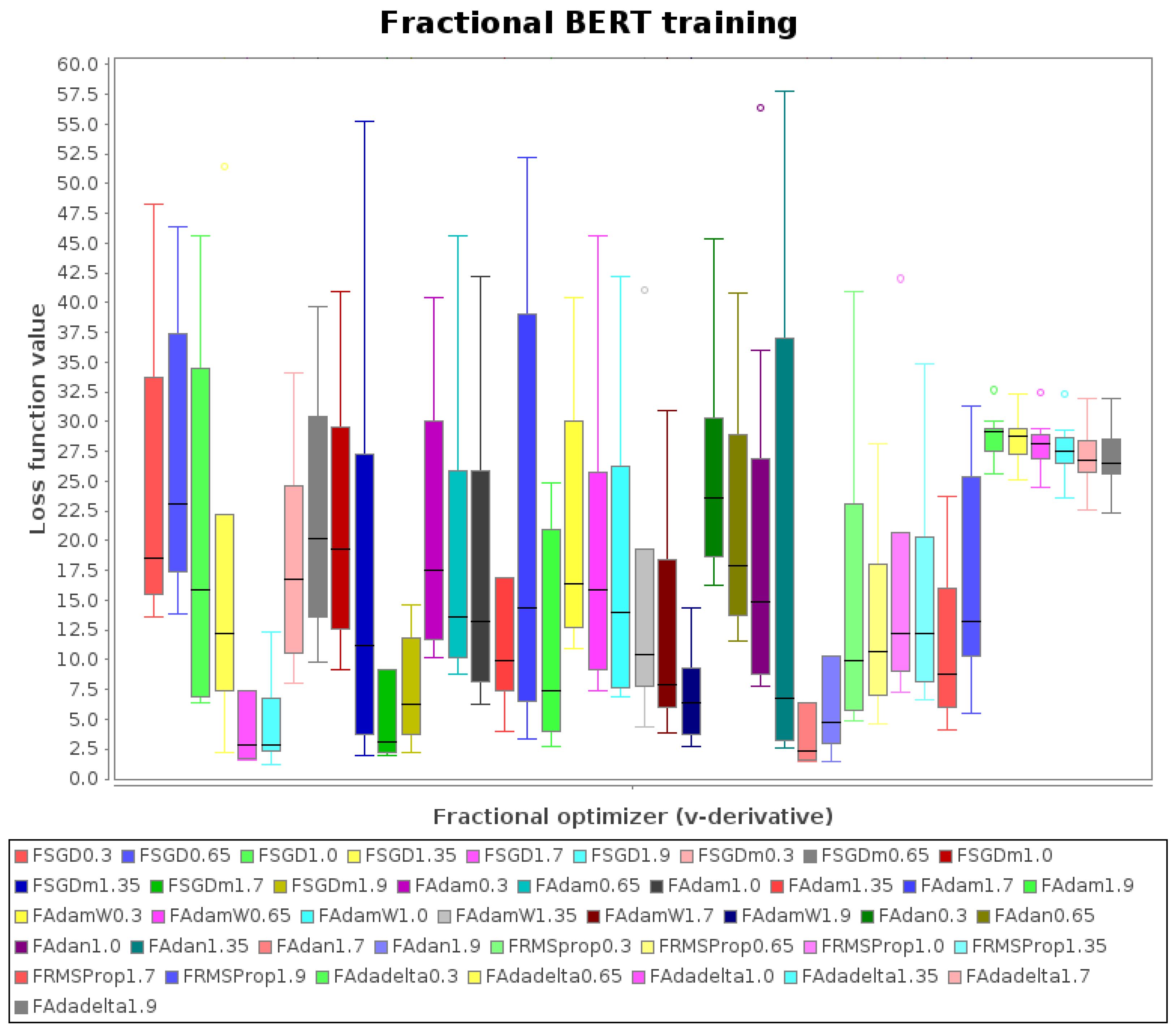
• Focused on FAdam, and considering the original experiment with Adam (i.e., FAdam with $\nu =1.0$), it is suboptimal and is outperformed by others with fractional derivatives
• Focused on FSGD and FSGDm, the best results are for $\nu =1.7$ and $1.9$
• Focused on FAdan, the best results are for $\nu =1.7$ and $1.9$
• FRMSProp and FAdadelta do not show a competitive performance
• From all the 42 bars in the boxplot, the best results are for FSGD, FSGDm, and FAdam, and the minimum is for FSGD with $\nu =1.9$.

In addition to the fact that the best optimizers turned out to be fractional, they achieved better consistency in the boxplot with respect to others with $\nu =1.0$. The numerical data of Figure 9 were not included because of simplicity and space-saving.

Figure 9. Boxplot of loss functions for FBERT trained with fractional optimizers and $\nu =\{0.3,0.65,1.0,1.35,1.7$, $1.9\}$.

Figure 9. Boxplot of loss functions for FBERT trained with fractional optimizers and $\nu =\{0.3,0.65,1.0,1.35,1.7$, $1.9\}$.

The source code of all fractional optimizers of this paper are available for download.

4. Discussion

One of the optimizers considered state of the art in machine learning is Adam, along with “Adam-flavors”, which focus mainly on the history and self-tuning of hyperparameters, in particular of the learning rate. In contrast, this work focuses on applying the ancient but powerful concept of fractional derivative to give an additional degree of freedom to existing optimizers.

Two experiments were developed to show how the fractional versions of gradient-based optimizers could improve their performance on GAN and natural language applications with BERT.

For Experiment 1, it is worth mentioning that the author of the original program admits the complexity of finding a set of hyperparameters that gives satisfactory results with GAN+Adam over MNIST (SGD is not even considered by many authors). This paper shows that using Adam (i.e., FAdam with $\nu =1.0$) does not always lead to successful results, and on the contrary, SGD does (not for $\nu =1.0$ but $\nu >1.7$). With these encouraging results, there are reasons to affirm that fractional gradients favor controlled artificial creativity, useful in neural networks such as GAN.

In Experiment 2, the fractional BERT was successfully implemented. Certainly, it was not trained on a large data set because the objective was to appreciate and compare the influence of the fractional gradient. The running time for each combination of fractional optimizer and $\nu$-derivative was not prohibitive and were successfully executed with a single GPU.

The experimental results show that SGD can be as competitive as other optimizers, which can also improve their performance when considering the fractional gradient. Indeed, fractional SGD has shown better performance in artificial creativity applications with GAN and NLP applications with BERT.

In future work, with the current background, it is proposed to apply fractional optimizers on large data sets, with transfer-learning from pre-trained models, as well as explore other application areas.

An open research area is to study the existence of some optimal value of the fractional derivative given by the data, the self-tuning of the fractional $\nu$-value, as well as the use of other fractional derivatives definitions.

The source code of the fractional optimizers for PyTorch resulting from this work are available online with the aim of being used and improved. At the same time, we hope that more members of the AI community will learn, apply and see the benefits of applying fractional calculus concepts.

References

- Haykin, S.S. Neural Networks and Learning Machines, 3rd. ed.; Pearson Education: Upper Saddle River, NJ, USA, 2009. [Google Scholar]
- Schmidt, R.M.; Schneider, F.; Hennig, P. Descending through a Crowded Valley—Benchmarking Deep Learning Optimizers. In Proceedings of the Proceedings of the 38th International Conference on Machine Learning, PMLR, Virtual Event. 18–24 July 2021; Meila, M., Zhang, T., Eds.; 2021; Volume 139, pp. 9367–9376. [Google Scholar]
- Robbins, H.; Monro, S. A stochastic approximation method. Ann. Math. Stat. 1951, 400–407. [Google Scholar] [CrossRef]
- Kingma, D.P.; Ba, J. Adam: A Method for Stochastic Optimization. arXiv 2014, arXiv:1412.6980. [Google Scholar]
- Abdulkadirov, R.; Lyakhov, P.; Nagornov, N. Survey of Optimization Algorithms in Modern Neural Networks. Mathematics 2023, 11, 2466. [Google Scholar] [CrossRef]
- Tian, Y.; Zhang, Y.; Zhang, H. Recent Advances in Stochastic Gradient Descent in Deep Learning. Mathematics 2023, 11, 682. [Google Scholar] [CrossRef]
- Herrera-Alcántara, O. Fractional Derivative Gradient-Based Optimizers for Neural Networks and Human Activity Recognition. Appl. Sci. 2022, 12, 9264. [Google Scholar] [CrossRef]
- PyTorch-Contributors. TOPTIM: Implementing Various Optimization Algorithms. 2023. Available online: https://pytorch.org/docs/stable/optim.html (accessed on 1 May 2023).
- Paszke, A.; Gross, S.; Massa, F.; Lerer, A.; Bradbury, J.; Chanan, G.; Killeen, T.; Lin, Z.; Gimelshein, N.; Antiga, L.; et al. PyTorch: An Imperative Style, High-Performance Deep Learning Library. In Advances in Neural Information Processing Systems 32; Curran Associates, Inc.: Red Hook, NY, USA, 2019; pp. 8024–8035. [Google Scholar]
- Oldham, K.B.; Spanier, J. The Fractional Calculus; Academic Press [A Subsidiary of Harcourt Brace Jovanovich, Publishers]: New York, NY, USA; London, UK, 1974; Volume 111, p. xiii+234. [Google Scholar]
- Miller, K.; Ross, B. An Introduction to the Fractional Calculus and Fractional Differential Equations; Wiley: Hoboken, NJ, USA, 1993. [Google Scholar]
- Mainardi, F. Fractional Calculus and Waves in Linear Viscoelasticity, 2nd ed.; Number 2; World Scientific: Singapore, 2022; p. 628. [Google Scholar]
- Yousefi, F.; Rivaz, A.; Chen, W. The construction of operational matrix of fractional integration for solving fractional differential and integro-differential equations. Neural Comput. Applic 2019, 31, 1867–1878. [Google Scholar] [CrossRef]
- Gonzalez, E.A.; Petráš, I. Advances in fractional calculus: Control and signal processing applications. In Proceedings of the 2015 16th International Carpathian Control Conference (ICCC), Szilvasvarad, Hungary, 27–30 May 2015; pp. 147–152. [Google Scholar] [CrossRef]
- Henriques, M.; Valério, D.; Gordo, P.; Melicio, R. Fractional-Order Colour Image Processing. Mathematics 2021, 9, 457. [Google Scholar] [CrossRef]
- Pang, G.; Lu, L.; Karniadakis, G.E. fPINNs: Fractional Physics-Informed Neural Networks. SIAM J. Sci. Comput. 2019, 41, A2603–A2626. [Google Scholar] [CrossRef] [Green Version]
- Wang, J.; Wen, Y.; Gou, Y.; Ye, Z.; Chen, H. Fractional-order gradient descent learning of BP neural networks with Caputo derivative. Neural Netw. 2017, 89, 19–30. [Google Scholar] [CrossRef] [PubMed]
- Bao, C.; Pu, Y.; Zhang, Y. Fractional-Order Deep Backpropagation Neural Network. Comput. Intell. Neurosci. 2018, 2018, 7361628. [Google Scholar] [CrossRef] [PubMed]
- Wang, H.; Yu, Y.; Wen, G. Stability analysis of fractional-order Hopfield neural networks with time delays. Neural Netw. 2014, 55, 98–109. [Google Scholar] [CrossRef] [PubMed]
- Chollet, F.; Zhu, Q.; Rahman, F.; Lee, T.; Marmiesse, G.; Zabluda, O.; Qian, C.; Jin, H.; Watson, M.; Chao, R.; et al. Keras. 2015. Available online: https://keras.io/ (accessed on 1 May 2023).
- Abadi, M.; Agarwal, A.; Barham, P.; Brevdo, E.; Chen, Z.; Citro, C.; Corrado, G.S.; Davis, A.; Dean, J.; Devin, M.; et al. TensorFlow: Large-Scale Machine Learning on Heterogeneous Systems. 2015. Available online: https://tensorflow.org (accessed on 1 May 2023).
- Goodfellow, I.; Pouget-Abadie, J.; Mirza, M.; Xu, B.; Warde-Farley, D.; Ozair, S.; Courville, A.; Bengio, Y. Generative adversarial nets. In Proceedings of the Advances in Neural Information Processing Systems, Montreal, QC, Canada, 8–13 December 2014; pp. 2672–2680. [Google Scholar]
- Devlin, J.; Chang, M.W.; Lee, K.; Toutanova, K. BERT: Pre-training of Deep Bidirectional Transformers for Language Understanding. In Proceedings of the 2019 Conference of the North American Chapter of the Association for Computational Linguistics: Human Language Technologies, Volume 1 (Long and Short Papers); Association for Computational Linguistics, Minneapolis, MN, USA; 2019; pp. 4171–4186. [Google Scholar] [CrossRef]
- Garrappa, R.; Kaslik, E.; Popolizio, M. Evaluation of Fractional Integrals and Derivatives of Elementary Functions: Overview and Tutorial. Mathematics 2019, 7, 407. [Google Scholar] [CrossRef] [Green Version]
- Zeiler, M.D. ADADELTA: An Adaptive Learning Rate Method. arXiv 2012, arXiv:1212.5701. [Google Scholar] [CrossRef]
- Duchi, J.; Hazan, E.; Singer, Y. Adaptive Subgradient Methods for Online Learning and Stochastic Optimization. J. Mach. Learn. Res. 2011, 12, 2121–2159. [Google Scholar]
- Zhuang, Z.; Liu, M.; Cutkosky, A.; Orabona, F. Understanding adamw through proximal methods and scale-freeness. arXiv 2022, arXiv:2202.00089. [Google Scholar]
- Tieleman, T.; Hinton, G. Neural Networks for Machine Learning; Technical Report; COURSERA: Napa County, CA, USA, 2012. [Google Scholar]
- Hochreiter, S.; Schmidhuber, J. Long short-term memory. Neural Comput. 1997, 9, 1735–1780. [Google Scholar] [CrossRef] [PubMed]
- Seo, J.D. Only Numpy: Implementing GAN (General Adversarial Networks) and Adam Optimizer Using Numpy with Interactive Code. 2023. Available online: https://towardsdatascience.com/only-numpy-implementing-gan-general-adversarial-networks-and-adam-optimizer-using-numpy-with-2a7e4e032021 (accessed on 1 May 2023).
- Deng, L. The mnist database of handwritten digit images for machine learning research. IEEE Signal Process. Mag. 2012, 29, 141–142. [Google Scholar] [CrossRef]
- Barla, N. How to code BERT using PyTorch. Available online: https://neptune.ai/blog/how-to-code-bert-using-pytorch-tutorial (accessed on 1 May 2023).
Disclaimer/Publisher’s Note: The statements, opinions and data contained in all publications are solely those of the individual author(s) and contributor(s) and not of MDPI and/or the editor(s). MDPI and/or the editor(s) disclaim responsibility for any injury to people or property resulting from any ideas, methods, instructions or products referred to in the content. |
© 2023 by the authors. Licensee MDPI, Basel, Switzerland. This article is an open access article distributed under the terms and conditions of the Creative Commons Attribution (CC BY) license (https://creativecommons.org/licenses/by/4.0/).
Share and Cite
Herrera-Alcántara, O.; Castelán-Aguilar, J.R. Fractional Gradient Optimizers for PyTorch: Enhancing GAN and BERT. Fractal Fract. 2023, 7, 500. https://doi.org/10.3390/fractalfract7070500
Herrera-Alcántara O, Castelán-Aguilar JR. Fractional Gradient Optimizers for PyTorch: Enhancing GAN and BERT. Fractal and Fractional. 2023; 7(7):500. https://doi.org/10.3390/fractalfract7070500
Chicago/Turabian StyleHerrera-Alcántara, Oscar, and Josué R. Castelán-Aguilar. 2023. "Fractional Gradient Optimizers for PyTorch: Enhancing GAN and BERT" Fractal and Fractional 7, no. 7: 500. https://doi.org/10.3390/fractalfract7070500
APA StyleHerrera-Alcántara, O., & Castelán-Aguilar, J. R. (2023). Fractional Gradient Optimizers for PyTorch: Enhancing GAN and BERT. Fractal and Fractional, 7(7), 500. https://doi.org/10.3390/fractalfract7070500