Abstract
The symmetric regularized long wave (SRLW) equation is a mathematical model used in many areas of physics; the solution of the SRLW equation can accurately describe the behavior of long waves in shallow water. To approximate the solutions of the equation, a time two-mesh (TT-M) decoupled finite difference numerical scheme is proposed in this paper to improve the efficiency of solving the SRLW equation. Based on the time two-mesh technique and two time-level finite difference method, the proposed scheme can calculate the velocity and density in the SRLW equation simultaneously. The linearization process involves a modification similar to the Gauss-Seidel method used for linear systems to improve the accuracy of the calculation to obtain solutions. By using the discrete energy and mathematical induction methods, the convergence results with in the discrete -norm for and in the discrete -norm for are proved, respectively. The stability of the scheme was also analyzed. Finally, some numerical examples, including error estimate, computational time and preservation of conservation laws, are given to verify the efficiency of the scheme. The numerical results show that the new method preserves conservation laws of four quantities successfully. Furthermore, by comparing with the original two-level nonlinear finite difference scheme, the proposed scheme can save the CPU time.
1. Introduction
The regularized long wave (RLW) equation [1,2] is a nonlinear partial differential equation that mainly describes the evolution of waves in shallow water channels and ion acoustics, etc. It is a simplified version of the more complex Korteweg-de Vries (KdV) equation [3], which includes higher-order nonlinearities and dispersion effects. The symmetric regularized long wave (SRLW) equation [4] is a modified version of the RLW equation that includes a symmetry-breaking term. This term allows for the formation of asymmetric solutions, making the SRLW equation a more realistic model for waves in shallow water channels.
In this paper, the following initial boundary value problem of the SRLW equation is considered:
where and are the fluid velocity and the density, respectively.
The SRLW equation has attracted significant attention and has been extensively studied in the literature. The existence of global attractors of the SRLW equation was studied in [5]. The travelling and solitary wave solutions of the SRLW equation were investigated by several methods including the exp-function method [6], the ()-expansion method [7,8], the tanh-function method [9,10], the Lie symmetry approach [11], the extended simple equation method [12], the analytical method [13], the tan ()-expansion method [14] and the sine–cosine method [15]. In [16,17], the spectral method and the Fourier pseudo-spectral method with a constraint operator were developed as approximations for the nonlinear term of the SRLW equation. Numerical solutions to the SRLW equation have also been studied by numerous methods, ranging from conservative finite difference schemes to mixed finite element methods. In their study, Wang et al. [18] introduced three conservative finite difference schemes that achieve second-order accuracy in both spatial and temporal domains. Their results indicate that each scheme is able to preserve energy conservation, but only the first scheme is capable of preserving mass conservation. Yimnet et al. [19] presented a novel finite difference method for the SRLW equation that utilizes a four-level average difference technique for solving the fluid velocity independently from the density. A coupled conservative three-level implicit scheme achieving fourth-order convergence rate was developed by Hu et al. [20]. Li [21] considered a weighted and compact conservative difference scheme that is decoupled and linearized in practical computation, thus requiring only the solution of two tridiagonal systems of linear algebraic equations at each time step. Bai et al. [22] investigated a two-layer conservative finite difference scheme for the SRLW equation with homogeneous boundary conditions and analyzed the scheme’s convergence and stability using a discrete functional analysis method. Xu et al. [23] applied a mixed finite element method to solve the dissipative SRLW equations with damping term. He et al. [24] developed a fourth-order accurate compact difference scheme for the SRLW equation for a single nonlinear velocity form and conducted theoretical analysis using the discrete energy method.
In terms of numerical computation, the time two-mesh (TT-M) method, when combined with either the finite element method or the finite difference method, offers better computational efficiency in solving a broad range of nonlinear partial differential equations. For instance, Liu et al. [25] proposed the fast TT-M finite element method for solving the fractional water wave model and applied it successfully to other fractional models. Yin et al. [26] developed a TT-M finite element algorithm for solving a space fractional Allen-Cahn model and analyzed the problem of parameter selection in detail. The TT-M finite element method was also leveraged by Liu et al. [27] to numerically solve the 2D Gray-Scott model with space fractional derivatives. A nonlinear distributed order diffusion model was efficiently solved using the TT-M algorithm in conjunction with the -Galerkin mixed finite element method by Wen et al. [28], both smooth and non-smooth solutions were considered. Additionally, Tian et al. [29] developed a finite element method equipped with the TT-M technique to solve the coupled Schrödinger-Boussinesq equations. Moreover, some studies have investigated combining the TT-M and finite difference methods to solve nonlinear fractional partial differential equations, such as the works of Qiu and Xu et al. [30,31], who proposed and analyzed a TT-M algorithm based on finite difference methods. The TT-M technique was also employed by Niu et al. [32] to develop a fast high-order compact difference scheme for the nonlinear distributed order fractional Sobolev model in porous media. Furthermore, He et al. [33] extended the application of the TT-M method by studying a primary scheme of second-order convergence in time and fourth-order in space for solving the nonlinear Schrödinger equation with a time two-mesh high-order compact difference scheme. Despite the extensive research on the TT-M method in various fields, to the best of our knowledge, no study on the application of the TT-M method combined with finite difference to the SRLW equation has been discovered. Hence, investigations on the TT-M finite difference method’s performance when applied to the SRLW equation are still required.
The SRLW Equation (1) is a coupled system and most existing schemes found in the literature are also coupled and require nonlinear implementation, which results in prolonged CPU processing time. The objective of this paper is to develop a novel difference scheme that offers the following three main advantages for solving the SRLW equation: (i) Based on the time two-mesh technique, we proposed a scheme that achieves decoupling and the nonlinear term of the system is linearized by using Taylor’s formula for a function with three variables, which is different from the literature [32,33]. In [32,33], the time two-mesh scheme is formulated by using Taylor’s formula for a function with one or two variables. As a result, our scheme becomes a linearized system in approximate numerical solution and can reduce the computational time. (ii) The scheme’s convergence and stability have been verified through detailed proof, and the theoretical analysis process is more complex than that of existing methods, since the linearized scheme contains a function of three variables. (iii) The linearization process involves a modification similar to the Gauss-Seidel method used for linear systems to improve the accuracy of the calculation for solutions. The conservation law of four quantities is preserved in the new scheme at the discrete level.
The remaining part of this article is organized as follows. In Section 2, some notations and useful lemmas are given. In Section 3, the TT-M finite difference numerical scheme is presented. In Section 4, the convergence and stability of the scheme is analyzed. In Section 5, some numerical results are provided to test the theoretical results and computational efficiency of the scheme. Finally, in Section 6, we provide the conclusions of the paper.
2. Notations and Some Lemmas
As usual, the time interval and spatial interval are divided into N and J uniform partitions. The following notations will be used in this paper:
where denote the uniform time and spatial step length, respectively, , , superscript n denotes a quantity associated with the time level , subscript j denotes a quantity associated with space mesh point . In this paper, M denotes general constant, which may have a different value in a different place.
Since for or , we may assume for simplicity, where and are ghost points. Let denote the set of mesh functions defined on with boundary conditions . For any two mesh functions , we define the discrete inner product and norms as follows:
Next, we present some useful lemmas.
Lemma 1
(See [24]). For any mesh functions , we have
Lemma 2
(See [33,34]). Assume that a sequence of non-negative real numbers satisfying
then there has the inequality , where and τ are positive constants.
Lemma 3
(See [22,34]). For any discrete mesh function , there exists constants and , such that
3. The TT-M Finite Difference Scheme
In this paper, we studied a TT-M finite difference fast numerical method for the SRLW Equation (1). In order to give the TT-M finite difference scheme, firstly, the time interval is partitioned uniformly into P coarse time intervals and then each of them is divided into fine time intervals. The coarse time mesh with the nodes satisfying and the fine time mesh with the nodes satisfying , where and are the coarse time and the fine time step size, respectively.
Secondly, the truncation errors of the problem (1) are considered, let be the exact solutions of and in term of the point , then we have
By Taylor series expansion, we have
Next, based on Equations (2) and (3), a TT-M finite difference scheme for problem (1) is constructed with three steps.
Step 1: on the coarse time mesh, let be the numerical solutions of of and in term of the point , then the coarse time nonlinear finite difference scheme is given as
where
Step 2: based on the solutions at time levels obtained from step 1, we apply the Lagrange’s linear interpolation formula to compute at time levels and , we have
Remark 1.
The Equation (7) is only employed for theoretical analysis of the scheme. In numerical simulation, the coarse numerical solutions are not needed for computation since they are not used in step 3.
Step 3: based on all the coarse numerical solutions obtained in the first two steps, Taylor’s formula is used to construct a linearized system on the fine time mesh, which is expressed as follows. Let be the numerical solutions of and in term of the point on the fine time mesh, then
where and
are the three partial derivatives of with respect to .
Remark 2.
Our method, similarly to the Gauss-Seidel method applied to linear systems, has been modified in order to enhance the accuracy of fine mesh solutions by using in calculation.
4. Convergence Analysis and Stability of the TT-M Finite Difference Scheme
The focus of this section is on performing convergence analysis of the nonlinear system specifically on the coarse time mesh.
Theorem 1.
Suppose that the exact solutions to the initial boundary value problem Equation (1) is sufficiently smooth and let be the numerical solutions on the coarse time mesh. Then,
Proof.
The proof contains two cases. Firstly, we consider the case of , then . The initial and boundary condition satisfies
Taking the inner product (·, ·) on both sides of Equation (10) with , we have
where
Notice that
then substituting Equations (13)–(17) into (12), we have
From Cauchy–Schwarz inequality, we obtain
Using Lemma 1, the Equation (18) can be rewritten as
Similarly, taking the inner product (·, ·) on both sides of Equation (11) with , we obtain
From the Cauchy–Schwarz inequality, we have
Using Lemma 1, the Equation (20) can be rewritten as
Add Equations (19) and (21), we obtain
Let , then Equation (22) becomes
and obtain
By taking small enough so that , then
Summing from 0 to inequalities in Equation (23), we have
and using Lemma 2, we obtain
From Equation (24) and the initial and boundary condition, we have
Then using Lemma 3, we obtain
Secondly, we consider the case of and . Based on the Lagrange’s interpolation formula, we obtain
Subtracting Equation (27) from (6), we have
Subtracting Equation (28) from (7), we obtain
Using (25), (26) and triangle inequality, we conclude
We obtain the result of Theorem 1 by synthesizing the aforementioned two cases. □
Next, we give the convergence analysis of the scheme on the fine time mesh.
Theorem 2.
Suppose that the exact solutions to the initial boundary value problem Equation (1) is sufficiently smooth and let be the numerical solutions on the fine time mesh. Then,
Proof.
Assume , Subtracting Equation (8) from Equation (2) and Equation (9) from Equation (3), we obtain
where
and , are the second order partial derivatives of ,
Taking the inner product (·, ·) on both sides of Equation (29) with , we have
Using and , we obtain
Using Lemma 1 and the Cauchy–Schwarz inequality, we have
Substituting Equations (34) and (35) into (31), then
Taking the inner product (·, ·) on both sides of Equation (30) with , we obtain
Add Equations (37) and (38), we have
Let , then
and obtain
By taking small enough so that , then
Summing from 0 to inequalities in Equation (40), we obtain
Using Lemma 2, we obtain
From Equation (42) and the initial and boundary condition, we have
Using Lemma 3, it led to
This completes the proof of Theorem 2. □
Next, we prove stability of the scheme on the coarse time mesh.
Theorem 3.
Proof.
The proof contains two cases. Firstly, we consider the case of . Taking the inner product (·, ·) on both sides of Equation (4) with , we have
Taking the inner product (·, ·) on both sides of Equation (5) with , we obtain
Add Equations (45) and (46), we obtain
Let , then Equation (47) becomes
and obtain
By taking small enough so that , then
Summing from 0 to inequalities in Equation (48), we have
and using Lemma 2, we obtain
that is
Secondly, we consider the case of and . From Equations (6) and (7), we obtain
The results obtained in the aforementioned two cases mean that the solution of scheme (4)–(5) is stable on the coarse time mesh. This completes the proof of Theorem 3. □
Next, we present stability analysis of the scheme on the fine time mesh.
Theorem 4.
Proof.
Taking the inner product (·, ·) on both sides of Equation (8) with , we have
From the Cauchy–Schwarz inequality, we obtain
then substituting Equations (51)–(53) into (50), we have
Taking the inner product (·, ·) on both sides of Equation (9) with , we obtain
Add Equations (54) and (55), we obtain
Let , then combine with the result of Theorem 3, the Equation (56) becomes
and obtain
By taking small enough so that , then
Summing from 0 to inequalities in Equation (57), we obtain
and then
Using Lemma 2, we obtain
that is
Notice that , , then
which indicates that the solution of scheme (8)–(9) is stable on the fine time mesh. This completes the proof of Theorem 4. □
5. Numerical Results
This section provides some numerical examples aimed at demonstrating the accuracy and computational time of the TT-M finite difference scheme that was discussed in Section 3. All simulations were implemented using a Intel(R) i7-10710U 1.61 GHz CPU and 16 GB memory personal computer running Windows 10 and Matlab R2019b. The SRLW equation is represented in the following formation:
and consider the following initial conditions
The exact solitary wave solution [4] of the SRLW Equation (1) has the following form
which takes the form of
when we set .
Next, we presented some values of error, convergence rate, conservation laws and long time simulation of the proposed scheme.
5.1. Error and Convergence Rate
We define the error and convergence rate by the following formula:
where m represents the TT-M finite difference scheme or the standard nonlinear finite difference (SNFD) scheme in [22]. We set in the whole numerical illustration process.
In order to illustrate the advantage of this approach, we calculated the error, convergence rate and computational time of the presented scheme and compared these numerical results with those obtained from scheme in [22]. Table 1 and Table 2 present discrete norm errors, the corresponding convergence rates and the time cost for both the TT-M finite difference scheme and the SNFD scheme in [22] under and , respectively. We recorded the error of both schemes at the final time for various mesh steps. The results from the new scheme show nearly identical important values as those obtained by the SNFD scheme in [22]. In term of the convergence rate, the results indicate that both the TT-M finite difference scheme and the SNFD scheme achieve approximately second-order convergence in space when and first-order in time when , which confirming the theoretical results in Theorem 2. Especially, the proposed scheme achieves a remarkable reduction in computation time of over 30 percent as compared to the SNFD scheme under and nearly half the computational time of the SNFD scheme under . The obtained results demonstrate a clear improvement achieved by our scheme over the previous method reported by [22].

Table 1.
The errors and convergence rates with .
Table 2.
The errors and convergence rates with .
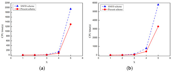
The 3D images of numerical solutions of and computed by the present scheme were shown in Figure 1. From the graph, one can see the propagation state of waves over a period of time. Figure 2 illustrates the exact and numerical solutions of and at obtained by the present scheme. It is evident that our numerical solutions exhibit an excellent correspondence with the exact solution. Furthermore, the CPU times of the two schemes are plotted in Figure 3 under and , respectively. From the figure, it is also can be seen that the present scheme can significantly decrease computation time. To sum up, compared with the method in [22], the scheme proposed in this paper not only ensures error and convergence order, but also greatly reduces computational time.
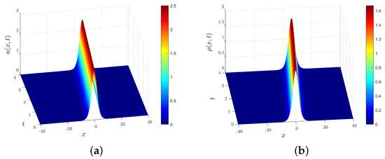
Figure 1.
Three−dimensional images of (a) and (b) with .
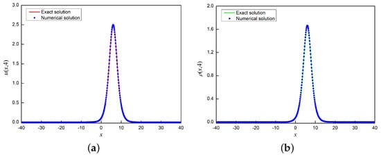
Figure 2.
Exact and numerical solution of (a) and (b) at with .
5.2. Conservative Approximations
To further verify the accuracy of the new scheme, we calculate four conservation laws of the SRLW Equation (1), such as:
Afterwards, employing discrete forms, we are able to compute four approximate conservative quantities which can be represented as
The values of four quantities are recorded in Table 3, Table 4, Table 5 and Table 6. In Table 3 and Table 4, regardless of the time step and grid spacing, the quantities and remain well-preserved at various times. In Table 5, for the case and , one can see that the quantity experiences a slight increase as time increases, however, as the spatial and temporal step sizes decrease, the variation of becomes extremely small. In Table 6, it has been found that for quantity , there was a minor decline under different mesh steps, but it gradually rebounded over time. Meanwhile, as the spatial and temporal step sizes decrease, the increases slightly. Figure 4 plots the variation curves of four quantities for the case and , which visually demonstrate that our scheme preserves the four conservation laws.
Table 3.
Quantity under different mesh steps h and at various times.
Table 4.
Quantity under different mesh steps h and at various times.
Table 5.
Quantity under different mesh steps h and at various times.
Table 6.
Quantity under different mesh steps h and at various times.
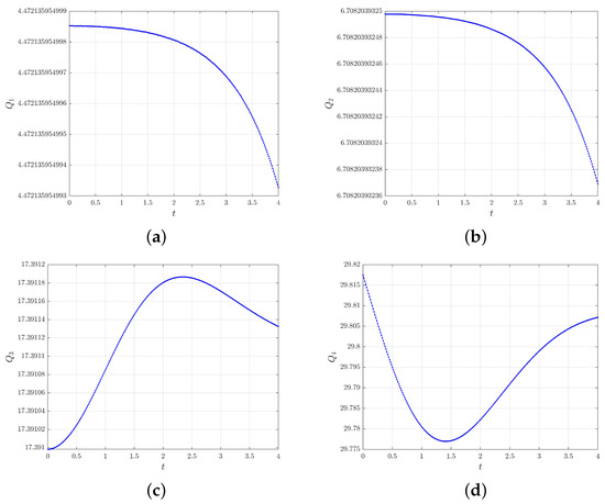
Figure 4.
Quantities (a), (b), (c) and (d) under mesh steps , .
5.3. Long-Time Simulation
Using the parameters , , , and , the long time waveforms of and generated by the present scheme are illustrated in Figure 5. The waveforms at t = 20 and 40 demonstrate a significant level of agreement with the waveforms at t = 0, which also indicates the accuracy of the scheme. Figure 6 displays the computational times of both the SNFD scheme and proposed scheme at long time. From the graph, it can be seen that the computational time difference between the two schemes grows increasingly as the simulation time increases, which indicates that the longer the simulation time, the more computational time can be saved by the scheme proposed in this paper. This once again proves the advantage of our scheme compared to the SNFD scheme in [22].
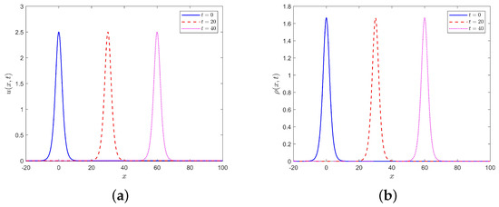
Figure 5.
Numerical solutions of (a) and (b) at long time with .
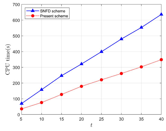
Figure 6.
Comparison of computation times of the SNFD scheme in [22] with present scheme at long time under .
6. Conclusions
This paper presents a new time two-mesh finite difference scheme for solving the symmetric regularized long wave equation, which contains a nonlinear derivative term in its formulation. Based on the previous work, our aim is to obtain a scheme that is not only error-preserving but also can save more computational time compared to the scheme in [22]. To achieve this goal, we have constructed a TT-M finite difference scheme that mainly consists of three steps. Firstly, the time interval is divided into coarse and fine time meshes, then the nonlinear system is solved on the coarse time mesh; secondly, coarse numerical solutions on the fine time mesh are computed using an interpolation formula based on the solutions derived in the step one; lastly, the nonlinear term of the SRLW equation is linearized using Taylor’s formula for a function with three variables and constructed the TT-M finite difference linear numerical scheme on the fine time mesh. In terms of theoretical results, we investigated the convergence and stability of numerical solutions. We observed that the solutions obtained from our proposed scheme converged to the exact solutions of the SRLW equation, and the rate of convergence is . Additionally, and h are sufficiently small, then the proposed scheme (8)–(9) is stable with respect to the initial conditions on the fine time mesh. The numerical results demonstrated that the proposed method effectively supported the analysis of the convergence rate. Meanwhile, one can observe that the errors of and in both the SNFD scheme in [22] and the present scheme are nearly identical, but the proposed scheme can reduce the computational time compared with the SNFD scheme. In addition, we calculated four conservation laws of the SRLW equation, regardless of the time step and grid spacing; the four quantities remain well-preserved at various times. The long time simulation example of the proposed scheme is also conducted in this part, the result shows that the waveform always maintains its original state in a long time. The error increases gently as simulation time is extended, which is a limitation of the proposed scheme and it will be improved by other methods in our future work. These findings demonstrate that the proposed method is more effective and yields a better improvement in solving the SRLW equation.
Author Contributions
Conceptualization, J.G.; methodology, J.G.; software, J.G. and S.H.; validation, S.H., Q.B. and J.L.; formal analysis, J.G. and S.H.; writing—original draft preparation, J.G.; writing—review and editing, J.G. and S.H.; funding acquisition, S.H., Q.B and J.L. All authors have read and agreed to the published version of the manuscript.
Funding
This work is supported by National Natural Science Foundation of China (Nos. 12161034 and 11961022), Natural Science Foundation of Inner Mongolia (No. 2021MS01017), Natural Scientific Research Innovation Team of Hohhot Minzu College (No. HMTD202005).
Institutional Review Board Statement
Not applicable.
Informed Consent Statement
Not applicable.
Data Availability Statement
All the data were computed using our method.
Acknowledgments
We are grateful to the anonymous reviewers for their valuable suggestions and comments.
Conflicts of Interest
The author declare no conflict of interest.
References
- Peregrine, D.H. Calculations of the development of an undular bore. J. Fluid Mech. 1966, 25, 321–330. [Google Scholar] [CrossRef]
- Peregrine, D.H. Long waves on beach. J. Fluid Mech. 1967, 27, 815–827. [Google Scholar] [CrossRef]
- Korteweg, D.J.; de Vries, G. On the change of form of long waves advancing in a rectangular canal, and on a new type of long stationary waves. Philos. Mag. 1895, 39, 422–443. [Google Scholar] [CrossRef]
- Seyler, C.E.; Fenstermacher, D.L. A symmetric regularized-long-wave equation. Phys. Fluids 1984, 27, 4–7. [Google Scholar] [CrossRef]
- Fang, S.; Guo, B.; Qiu, H. The existence of global attractors for a system of multi-dimensional symmetric regularized wave equations. Commun. Nonlinear Sci. Numer. Simul. 2009, 14, 61–68. [Google Scholar]
- Xu, F. Application of Exp-function method to symmetric regularized long wave (SRLW) equation. Phys. Lett. A 2008, 372, 252–257. [Google Scholar] [CrossRef]
- Abazari, R. Application of (G′/G)-expansion method to travelling wave solutions of three nonlinear evolution equation. Comput. Fluids 2010, 39, 1957–1963. [Google Scholar] [CrossRef]
- Chand, F.; Malik, A.K. Exact traveling wave solutions of some nonlinear equations using(G′/G)-expansion method. Int. J. Nonlinear Sci. 2012, 14, 416–424. [Google Scholar]
- Yalçınkaya, İ.; Ahmad, H.; Tasbozan, O.; Kurt, A. Soliton solutions for time fractional ocean engineering models with Beta derivative. J. Ocean Eng. Sci. 2022, 7, 444–448. [Google Scholar] [CrossRef]
- Mamun, A.A.; Ananna, S.N.; An, T.; Shahen, N.H.M.; Asaduzzaman, M. Dynamical behaviour of travelling wave solutions to the conformable time-fractional modified Liouville and mRLW equations in water wave mechanics. Heliyon 2021, 7, e07704. [Google Scholar] [CrossRef]
- Hussain, A.; Jhangeer, A.; Abbas, N.; Khan, I.; Nisar, K.S. Solitary wave patterns and conservation laws of fourth-order nonlinear symmetric regularized long-wave equation arising in plasma. Ain Shams Eng. J. 2021, 12, 3919–3930. [Google Scholar] [CrossRef]
- Lu, D.; Seadawy, A.R.; Ali, A. Applications of exact traveling wave solutions of modified Liouville and the symmetric regularized long wave equations via two new techniques. Results Phys. 2018, 9, 1403–1410. [Google Scholar] [CrossRef]
- Manafian, J.; Zamanpour, I. Exact travelling wave solutions of the symmetric regularized long wave (SRLW) using analytical methods. Stat. Optim. Inf. Comput. 2014, 2014, 47–55. [Google Scholar]
- Sendi, C.T.; Manafian, J.; Mobasseri, H.; Mirzazadeh, M.; Zhou, Q.; Bekir, A. Application of the ITEM for solving three nonlinear evolution equations arising in fluid mechanics. Nonlinear Dyn. 2019, 95, 669–684. [Google Scholar] [CrossRef]
- Bekir, A. New solitons and periodic wave solutions for some nonlinear physical models by using the sine–cosine method. Phys. Scr. 2008, 77, 045008. [Google Scholar] [CrossRef]
- Guo, B. The spectral method for symmetric regularized wave equations. J. Comput. Math. 1987, 5, 297–306. [Google Scholar]
- Zheng, J.; Zhang, R.; Guo, B. The Fourier pseudo-spectral method for the SRLW equation. Appl. Math. Mech. 1989, 10, 801–810. [Google Scholar]
- Wang, T.C.; Zhang, L.M.; Chen, F.Q. Conservative schemes for the symmetric regularized long wave equations. Appl. Math. Comput. 2007, 190, 1063–1080. [Google Scholar] [CrossRef]
- Yimnet, S.; Wongsaijai, B.; Rojsiraphisal, T.; Poochinapan, K. Numerical implementation for solving the symmetric regularized long wave equation. Appl. Math. Comput. 2016, 273, 809–825. [Google Scholar] [CrossRef]
- Hu, J.S.; Zheng, K.L.; Zheng, M.B. Numerical simulation and convergence analysis of high-order conservative difference scheme for SRLW equation. Appl. Math. Model. 2014, 38, 5573–5581. [Google Scholar] [CrossRef]
- Li, S.G. Numerical study of a conservative weighted compact difference scheme for the symmetric regularized long wave equations. Numer. Methods Partial. Differ. Equ. 2019, 35, 60–83. [Google Scholar] [CrossRef]
- Bai, Y.; Zhang, L.M. A conservative finite difference scheme for symmetric regularized long wave equations. Acta Math. Appl. Sin. 2007, 30, 248–255. [Google Scholar]
- Xu, Y.C.; Hu, B.; Xie, X.P.; Hu, J.S. Mixed finite element analysis for dissipative SRLW equations with damping term. Phys. Fluids 2012, 218, 4788–4797. [Google Scholar] [CrossRef]
- He, Y.Y.; Wang, X.F.; Cheng, H.; Deng, Y.Q. Numerical analysis of a high-order accurate compact finite difference scheme for the SRLW equation. Appl. Math. Comput. 2022, 418, 126837. [Google Scholar] [CrossRef]
- Liu, Y.; Yu, Z.D.; Li, H.; Liu, F.W.; Wang, J.F. Time two-mesh algorithm combined with finite element method for time fractional water wave model. Int. J. Heat Mass Transf. 2018, 120, 1132–1145. [Google Scholar] [CrossRef]
- Yin, B.L.; Liu, Y.; Li, H.; He, S. Fast algorithm based on TT-M FE system for space fractional Allen-Cahn equations with smooth and non-smooth solutions. J. Comput. Phys. 2019, 379, 351–372. [Google Scholar] [CrossRef]
- Liu, Y.; Fan, E.Y.; Yin, B.L.; Li, H.; Wang, J.F. TT-M finite element algorithm for a two-dimensional space fractional Gray-Scott model. Comput. Math. Appl. 2020, 80, 1793–1809. [Google Scholar] [CrossRef]
- Wen, C.; Liu, Y.; Yin, B.L.; Li, H.; Wang, J.F. Fast second-order time two-mesh mixed finite element method for a nonlinear distributed-order sub-diffusion model. Numer. Algorithms 2021, 88, 523–553. [Google Scholar] [CrossRef]
- Tian, J.L.; Sun, Z.Y.; Liu, Y.; Li, H. TT-M Finite Element Algorithm for the Coupled Schrödinger–Boussinesq Equations. Axioms 2022, 11, 314. [Google Scholar] [CrossRef]
- Qiu, W.L.; Xu, D.; Guo, J.; Zhou, J. A time two-grid algorithm based on finite difference method for the two-dimensional nonlinear time-fractional mobile/immobile transport model. Numer. Algorithms 2020, 85, 39–58. [Google Scholar] [CrossRef]
- Xu, D.; Guo, J.; Qiu, W.L. Time two-grid algorithm based on finite difference method for two-dimensional nonlinear fractional evolution equations. Appl. Numer. Math. 2019, 152, 169–184. [Google Scholar] [CrossRef]
- Niu, Y.X.; Liu, Y.; Li, H.; Liu, F.W. Fast high-order compact difference scheme for the nonlinear distributed-order fractional Sobolev model appearing in porous media. Math. Comput. Simul. 2023, 203, 387–407. [Google Scholar] [CrossRef]
- He, S.; Liu, Y.; Li, H. A time two-mesh compact difference method for the one-dimensional nonlinear schrödinger equation. Entropy 2022, 24, 806. [Google Scholar] [CrossRef] [PubMed]
- Zhou, Y.L. Application of Discrete Functional Analysis to the Finite Difference Method; International Academic Publishers: Beijing, China, 1990. [Google Scholar]
Disclaimer/Publisher’s Note: The statements, opinions and data contained in all publications are solely those of the individual author(s) and contributor(s) and not of MDPI and/or the editor(s). MDPI and/or the editor(s) disclaim responsibility for any injury to people or property resulting from any ideas, methods, instructions or products referred to in the content. |
© 2023 by the authors. Licensee MDPI, Basel, Switzerland. This article is an open access article distributed under the terms and conditions of the Creative Commons Attribution (CC BY) license (https://creativecommons.org/licenses/by/4.0/).