Impact of Lévy Noise with Infinite Activity on the Dynamics of Measles Epidemics

Abstract

This research article investigates the application of Lévy noise to understand the dynamic aspects of measles epidemic modeling and seeks to explain the impact of vaccines on the spread of the disease. After model formulation, the study utilises uniqueness and existence techniques to derive a positive solution to the underlying stochastic model. The Lyapunov function is used to investigate the stability results associated with the proposed stochastic model. The model’s dynamic characteristics are analyzed in the vicinity of the infection-free and endemic states of the associated ODEs model. The stochastic threshold ${\mathbb{R}}_s$ that ensures disease’s extinction whenever ${\mathbb{R}}_s<1$ is calculated. We utilized data from Pakistan in 2019 to estimate the parameters of the model and conducted simulations to forecast the future behavior of the disease. The results were compared to actual data using standard curve fitting tools.

1. Introduction

The measles infection, also called rubella, is extremely contagious and spreads throughout the globe. It is caused by the virus Morbilli, related to the community of Paramyxoviridae [1,2]. Vaccination is a powerful tool in reducing the impact of the disease over time. However, the force of mortality continues to affect young children under the age of five [3]. Measles infects ten million children each year, and millions of them die due to factors such as the unavailability of a balanced diet, weak digestion, and pneumonia [4]. Disease spread is caused by personal contact, sneezing, coughing, and contact with airborne and nasal droplets. The virus stays active for approximately two hours, and remains highly contagious during this period. The initial symptoms of the disease include nasal discharge, sore throat, and the presence of small white spots on the tongue. In later stages, coughing may occur. The typical incubation period for this infection is about four days before the appearance of the rash, and lasts for nearly five days after the rash appears. The mean incubation time is about fourteen or fifteen days, changing with external factors such as the environment and weather of the surroundings [5]. In real practice, vaccinated people may suffer side-effects, or it may be the case that vaccines are not available. On the other hand, vaccination acts as a preventive measure against measles, reducing the incidence rate by up to 73% over the past eighteen years. According to the World Health Organisation, Measles is present in many developed countries around the world, particularly in Asia and Africa. More than one hundred and fifty thousand people died due to measles in 2018. In the meantime, the death to infection ratio has decreased by about 85 percent [6,7]. According to reports from the WHO, nearly 110,000 people died in 2017 due to measles, with a majority of them being children under six years old. This highlights the need for effective and safe vaccination [8]. The discovery of vaccines for infectious diseases has lowered the ratio of death and infection to a large extent. This process saves about three hundred thousand individuals from death each year. Vaccines produce antibodies that act against reinfection and strengthen the immune system [9]. Specifically, measles can be controlled by the MMR vaccines. These vaccines are considered very safe for both children and the elderly, and can reduce the severity of measles infection to a great extent. According to studies, one dose of the MMR vaccine can prevent disease in around 91% of cases, while two doses can provide approximately 95% protection. Other diseases such as the mumps can be controlled by this vaccine as well [10]. Nigeria experiences periodic outbreaks of measles, as the disease is endemic in the country. The disease spreads in Nigeria during all seasons of the year, and is highly contiguous during dry weather.

In addition, Pakistan is among the countries in the WHO’s Eastern Mediterranean Region most highly burdened by measles [11]. Over the past 9 to 12 years, there has been a sharp increase in measles outbreaks throughout Pakistan; some 2845 cases of measles were reported in Pakistan in 2016. This number increased to 6791 in 2017 and 33,007 in 2018, which represents approximately 43%, 21%, and 50% of all cases reported in the Eastern Mediterranean region comprising 23 countries [11]. Nearly 129 children died from measles in 2017, and in 2018 the number increased to about 300 [12].

Mathematical modeling is regarded as a significant and powerful approach for examining and forecasting the dynamic patterns of epidemics [7,12,13,14]. Most of the models used to date employ the integer order derivative, and their analysis is related to classical theory. The foundation of a mathematical modeling relies heavily on the availability of biological information and data regarding the epidemic under consideration. Mathematical models for the measles have wide application for understanding its spreading dynamics and controlling it. White noise plays a vital role in explaining the dynamics of physical and biological problems. The impact of external environmental factors such as white noise on the dynamics of measles epidemics is significant [15]. Due to the non-homogeneity and nonlinearity of population interactions and other complexities, epidemic prediction cannot be depicted using traditional modeling approaches. Moreover, the dynamics and control of various epidemics may be affected by global environmental factors.

The human population is subject to many complex and random variations in the real world. Therefore, stochastic models are a more appropriate technique for modelling epidemics. It has been demonstrated that stochastic models are more realistic compared to deterministic models. Several researchers have recently focused on perturbations that can capture the true dynamics of the epidemic based on stochastic modelling [13,15,16]. The Lévy white noise is important at various velocities for the spacing of threshold parameters. Adding Lévy noise terms can lead to more realistic and accurate results in stochastically analyzed models for various infectious diseases. The stochastic version of the underlying deterministic mode can be obtained by including this noise in the aforementioned systems. Typically, two types of noise are utilized in such models, namely, Lévy noise and Gaussian noise. The Lévy noise is more suitable than the Gaussian noise because the resulting system is able to model systems with a higher degree of complexity [16,17,18,19]. Due to fluctuations in diffusion problems, disturbances cannot be described by the continuous stochastic model; thus, it is important to model these phenomena using jump processes. For this reason, we consider the problem using Lévy noise.

The remainder of this manuscript is structured as follows. In Section 2, we propose a model based on random processes for the transmission dynamics of measles. In Section 3, we present the dynamic features of the globalized positive model’s solution. In Section 4 and Section 5, we obtain necessary conditions related to disease elimination and persistence of the proposed stochastic model. We optimize the proposed problem using the cases of measles infection in the population of Pakistan for January to October 2019 in Section 6. In Section 7, we verify the theory behind the obtained results qualitatively and quantitatively, and provide numerical simulations. Finally, we conclude our analysis in Section 8 with remarks and recommendations for future research work.

2. Model Formulation

Olumuyiwa et al. [20] recently developed a mathematical model for describing the infection dynamics of the epidemic measles by using a deterministic approach. The authors employed the epidemiological concept of population and divided the entire human population into six classes, including susceptible, vaccinated, exposed, infectious, hospitalised, and recovered individuals, respectively denoted by $\mathbb{S}\left(t\right)$, $\mathbb{V}\left(t\right)$, $\mathbb{E}\left(t\right)$, $\mathbb{I}\left(t\right)$, $\mathbb{H}\left(t\right)$, and $\mathbb{R}\left(t\right)$. The addition to the susceptible population per day is provided by the rate $\varphi$. The vulnerable class is subject to a vaccination rate $\tau$ and loses immunity against the disease at a rate $\omega$, which is commonly known as the “waning rate of vaccination”. The rate of infection for the susceptible class is denoted by $\alpha$. Therefore, the term $\alpha \mathbb{S}\mathbb{I}$ represents the total infection rate per time unit. Additionally, the transition from the exposed class to the infected class is represented by $\beta$. Individuals in the infected population are hospitalized at a rate $\rho$ and then recover from measles at a rate $\gamma$. The model assumes a constant natural death rate, denoted by $\mu$, for all population classes. In addition, the infection-related death rate is provided by the parameter $\delta$. Here, we do not assume any natural recovery from measles infection. The model chart is illustrated in Figure 1 [21]. The mathematical formulation of the above discussion can be converted into a model of ordinary differential equations (ODEs), represented in symbolic form as follows:

$$\begin{array}{cc}\hfill \frac{d\mathbb{S}\left(t\right)}{t}& =-\alpha \mathbb{I}\left(t\right)\mathbb{S}\left(t\right)+\varphi -(\mu +\tau )\mathbb{S}\left(t\right)+\omega \mathbb{V}\left(t\right),\hfill \\ \hfill \frac{d\mathbb{V}\left(t\right)}{t}& =-(\omega +\mu )\mathbb{V}\left(t\right)+\tau \mathbb{S}\left(t\right),\hfill \\ \hfill \frac{d\mathbb{E}\left(t\right)}{t}& =-(\beta +\mu )\mathbb{E}\left(t\right)+\alpha \mathbb{I}\left(t\right)\mathbb{S}\left(t\right),\hfill \\ \hfill \frac{d\mathbb{I}\left(t\right)}{t}& =-(\mu +\rho +\delta )\mathbb{I}\left(t\right)+\beta \mathbb{E}\left(t\right),\hfill \\ \hfill \frac{d\mathbb{H}\left(t\right)}{t}& =-(\mu +\gamma +\delta )\mathbb{H}\left(t\right)+\rho \mathbb{I}\left(t\right),\hfill \\ \hfill \frac{d\mathbb{R}\left(t\right)}{t}& =-\mu \mathbb{R}\left(t\right)+\gamma \mathbb{H}\left(t\right).\hfill \end{array}$$

(1)

The threshold parameter for the model (1) is obtained using standard techniques, and has the following form:

$${\mathbb{R}}_0^D=\frac{(\mu +\omega )\varphi \beta \alpha }{(\mu +\beta )(\mu +\delta +\rho )(\mu +\omega +\tau )\mu }.$$

(2)

The main theme of the present manuscript is to modify model (1) by including white and Lévy noise as well as the incidence rate of nonlinear shapes; the white noise is used for the continuity part and the Lévy noise for the jumping part. The extended form of the deterministic system can be written in stochastic form as follows:

$$\begin{array}{cc}\hfill d\mathbb{S}& =\left[\varphi -\frac{\alpha \mathbb{S}\left(t\right)\mathbb{I}\left(t\right)}{\mathbb{N}\left(t\right)}+\omega \mathbb{V}\left(t\right)-(\tau +\mu )\mathbb{S}\left(t\right)\right]dt+{\xi }_1\mathbb{S}\left(t\right)d{\mathbb{W}}_1\left(t\right)+{\int }_Y{\mathbb{X}}_1\left(y\right)\mathbb{S}\left(t^{-}\right)\tilde{\mathbb{N}}(dt,dy),\hfill \\ \hfill d\mathbb{V}& =\left[\tau \mathbb{S}\left(t\right)-(\mu +\omega )\mathbb{V}\left(t\right)\right]dt+{\xi }_2\mathbb{V}d{\mathbb{W}}_2\left(t\right)+{\int }_Y{\mathbb{X}}_2\left(y\right)\mathbb{V}\left(t^{-}\right)\tilde{\mathbb{N}}(dt,dy),\hfill \\ \hfill d\mathbb{E}& =\left[\frac{\alpha \mathbb{S}\left(t\right)\mathbb{I}\left(t\right)}{\mathbb{N}\left(t\right)}-(\mu +\beta )\mathbb{E}\left(t\right)\right]dt+{\xi }_3\mathbb{E}\left(t\right)d{\mathbb{W}}_3\left(t\right)+{\int }_Y{\mathbb{X}}_3\left(y\right)\mathbb{E}\left(t^{-}\right)\tilde{\mathbb{N}}(dt,dy),\hfill \\ \hfill d\mathbb{I}& =\left[\beta \mathbb{E}\left(t\right)-(\rho +\delta +\mu )\mathbb{I}\left(t\right)\right]dt+{\xi }_4\mathbb{I}\left(t\right)d{\mathbb{W}}_4\left(t\right)+{\int }_Y{\mathbb{X}}_4\left(y\right)\mathbb{I}\left(t^{-}\right)\tilde{\mathbb{N}}(dt,dy),\hfill \\ \hfill d\mathbb{H}& =\left[\rho \mathbb{I}\left(t\right)-(\gamma +\delta +\mu )\mathbb{H}\left(t\right)\right]dt+{\xi }_5\mathbb{I}\left(t\right)d{\mathbb{W}}_5\left(t\right)+{\int }_Y{\mathbb{X}}_5\left(y\right)\mathbb{H}\left(t^{-}\right)\tilde{\mathbb{N}}(dt,dy),\hfill \\ \hfill d\mathbb{R}& =\left[\gamma \mathbb{H}\left(t\right)-\mu \mathbb{R}\left(t\right)\right]dt+{\xi }_6\mathbb{R}\left(t\right)d{\mathbb{W}}_6\left(t\right)+{\int }_Y{\mathbb{X}}_6\left(y\right)\mathbb{R}\left(t^{-}\right)\tilde{\mathbb{N}}(dt,dy),\hfill \end{array}$$

(3)

where ${\mathbb{W}}_i\left(t\right)$ for $i=1,\cdots ,6$ is standard Brownian motion defined in a complete probability space $(\Omega ,\mathbb{F},\mathbb{P})$ with filtration ${\left\{{\mathbb{F}}_t\right\}}_{t⩾0}$, satisfying the usual condition ${\xi }_1,{\xi }_2,{\xi }_3,{\xi }_4,{\xi }_5$, with ${\xi }_6$ representing the intensity of noise, $\mathbb{S}\left(t^{-}\right),\mathbb{V}\left(t^{-}\right),\mathbb{E}\left(t^{-}\right),\mathbb{I}\left(t^{-}\right),\mathbb{H}\left(t^{-}\right)$ and $\mathbb{R}\left(t^{-}\right)$ being the left limit of $\mathbb{S},\mathbb{V},\mathbb{E},\mathbb{I},\mathbb{H}$ and $\mathbb{R}$, respectively, $\tilde{\mathbb{N}}=\mathbb{N}(dt,dy)-v\left(dy\right)dt$ and $\mathbb{N}(dy,dt)$ a Poisson counting measure with characteristic measure $\nu$ on the measurable subset $\mathrm{Y}$ of $[0,\infty )$, and with $\nu \left(Y\right)<\infty$ and ${\mathbb{X}}_i:Z\times \Omega ⟶{\mathbb{R}}_{+},(\mathrm{i}=1,2,3,4,5,6)$ representing the effect of random jumps, which are assumed to be bounded and continuous with respect to $\nu$ and to be $\mathbb{B}\left(Y\right)\times {\mathbb{F}}_t$-measurable.

With regard to the model (3), in the present work we are particularly interested in answering the following questions:

Q₁:

Does the Lévy noise influence the dynamic properties of measles outbreaks?

Q₂:

How can contaminated vaccinations contribute to the spread of measles, and what measures are in place to prevent such incidents?

Q₃:

What criterion is used to determine the extinction of a disease?

Q₄:

What are the criteria that indicate the persistence of the system?

3. The Existence of a Positive Solution and Its Uniqueness

In this section, we intend to apply the techniques from [16] to establish a proof of the existence of a global and positive solution to the proposed stochastic model. To prove the existence and uniqueness of a solution of model (3), it is important to consider the following two conditions:

(C₁).

For every $\mathbb{Q}>0$ ∃ ${\mathbb{L}}_{\mathbb{Q}}>0$;

$${\int }_Y{\left|A_i\left(x_1,y\right)-A_i\left(x_2,y\right)\right|}^{2}v\left(dy\right)\le {\mathbb{L}}_{\mathbb{Q}}{\left|x_1-x_2\right|}^2,i=1,\cdots ,6,$$

(4)

for $\left|y_1\right|\vee \left|y_2\right|\le \mathbb{M}$; here,

$$\begin{array}{c}{A}_1(x,y)={\mathbb{X}}_1\left(y\right)x\mathrm{at}x=\mathbb{S}\left(t^{-}\right),\hfill \\ A_2(x,y)={\mathbb{X}}_2\left(y\right)x\mathrm{at}x=\mathbb{V}\left(t^{-}\right),\hfill \\ A_3(x,y)={\mathbb{X}}_3\left(y\right)x\mathrm{at}x=\mathbb{E}\left(t^{-}\right),\hfill \\ A_4(x,y)={\mathbb{X}}_4\left(y\right)x\mathrm{at}x=\mathbb{I}\left(t^{-}\right),\hfill \\ A_5(x,y)={\mathbb{X}}_5\left(y\right)x\mathrm{at}x=\mathbb{H}\left(t^{-}\right),\hfill \\ A_6(x,y)={\mathbb{X}}_6\left(y\right)x\mathrm{at}x=\mathbb{R}\left(t^{-}\right).\hfill \end{array}$$

(C₂).

$\left|log\left({\mathbb{X}}_i\left(x\right)\right)\right|\le C$ for ${\mathbb{X}}_i\left(x\right)>-1,i=1,\cdots ,6$, C is a positive constant.

Theorem 1.

For a given initial value $(\mathbb{S},\mathbb{V},\mathbb{E},\mathbb{I},\mathbb{H},\mathbb{R})\left(0\right)\in {\mathbb{R}}_{+}^6$, system (3) has one global root $(\mathbb{S},\mathbb{V},\mathbb{E},\mathbb{I},\mathbb{H},\mathbb{R})\left(t\right)\in {\mathbb{R}}_{+}^6$ for all $t\ge 0$ a.s.

Proof. 

Using $\left({\mathbb{C}}_1\right)$, the results due to drifted and the diffused terms are local Lipschitzian, for every initial conditions $(\mathbb{S},\mathbb{V},\mathbb{E},\mathbb{I},\mathbb{H},\mathbb{R})\left(0\right)\in {\mathbb{R}}_{+}^6$, ∃ a unique localized root $\left(\mathbb{S}\right(t),\mathbb{V}(t),\mathbb{E}(t),\mathbb{I}(t),\mathbb{H}(t),\mathbb{R}(t\left)\right)$ on $t\in [0,{\tau }_e)$, ${\tau }_e$ is the explosion time. To show that the solution is global, we have to prove that ${\tau }_e=\infty$ a.s. In the first attempt, we prove the condition that $\left(\mathbb{S}\right(t),\mathbb{V}(t),\mathbb{E}(t),\mathbb{I}(t),\mathbb{H}(t),\mathbb{R}(t\left)\right)$ are not approaching infinity in a finite duration of time. Let $k_0>0$ is too much large such that $\left(\mathbb{S}\right(0),\mathbb{V}(0),\mathbb{E}(0),\mathbb{I}(0),\mathbb{H}(0),\mathbb{R}(0\left)\right)$ lies in $[\frac{1}{k_0},k_0]$. For every integer value $k\le k_0$, consider the stopping time in the form of

$${\tau }_k=inf\left\{t\in \left[0,{\tau }_e\right)/(\mathbb{S}\left(t\right),\mathbb{V}\left(t\right),\mathbb{E}\left(t\right),\mathbb{I}\left(t\right),\mathbb{H}\left(t\right),\mathbb{R}\left(t\right))\notin \left(\frac{1}{k},k\right)\right\}.$$

(5)

Let $inf\varnothing =\infty$; from this, we can see that ${\tau }^{+}\le {\tau }_e,$ which implies that ${\tau }^{+}=\infty$ a.s showing ${\tau }_e=+\infty$ a.s. Considering that ${\tau }^{+}$ is less than ∞, there must exist a number $T>0$ such that $0<\mathbb{P}\left({\tau }^{+}<T\right)$.

Next, let us consider the operator $\mathbb{F}:{\mathbb{R}}_{+}^6\to {\mathbb{R}}_{+}$ from the $C^2$ set in the form of

$$\begin{array}{cc}\hfill \mathbb{F}(\mathbb{S},\mathbb{V},\mathbb{E},\mathbb{I},\mathbb{H},\mathbb{R})& =\mathbb{H}+\mathbb{V}+\mathbb{S}+\mathbb{I}+\mathbb{E}+\mathbb{R}-6-(\log \mathbb{S}+\log \mathbb{V}+\log \mathbb{E}+\log \mathbb{I}+\log \mathbb{H}+\log \mathbb{R}).\hfill \end{array}$$

(6)

Applying $It\widehat{o}$ formula to $\mathbb{F}$ for all $t\in [0,{\tau }^{+}]$, we have

$$\begin{array}{cc}\hfill d\mathbb{F}& =L\mathbb{F}(\mathbb{S},\mathbb{V},\mathbb{E},\mathbb{I},\mathbb{H},\mathbb{R})dt+{\xi }_1(\mathbb{S}-1)d{\mathbb{W}}_1\left(t\right)+x{i}_2(\mathbb{V}-1)d{\mathbb{W}}_2\left(t\right)\hfill \\ \hfill & +{\xi }_3(\mathbb{E}-1)d{\mathbb{W}}_3\left(t\right)+{\xi }_4(\mathbb{I}-1)d{\mathbb{W}}_4\left(t\right)+{\xi }_5(\mathbb{H}-1)d{\mathbb{W}}_5\left(t\right)+{\xi }_6(\mathbb{R}-1)d{\mathbb{W}}_6\left(t\right)\hfill \\ \hfill & +{\int }_{\mathsf{{\rm Y}}}\left[{\mathbb{X}}_1\left(y\right)\mathbb{S}-log\left({\mathbb{X}}_1\left(y\right)+1\right)\right]\tilde{\mathbb{N}}\left(d\chi \right)+{\int }_{\mathsf{{\rm Y}}}\left[{\mathbb{X}}_2\left(y\right)\mathbb{V}-log\left(1+{\mathbb{X}}_2\left(y\right)\right)\right]\tilde{\mathbb{N}}\left(d\chi \right)\hfill \\ \hfill & +{\int }_{\mathsf{{\rm Y}}}\left[{\mathbb{X}}_3\left(y\right)\mathbb{E}-log\left(1+{\mathbb{X}}_3\left(y\right)\right)\right]\tilde{\mathbb{N}}\left(d\chi \right)+{\int }_{\mathsf{{\rm Y}}}\left[{\mathbb{X}}_4\left(y\right)\mathbb{I}-log\left(1+{\mathbb{X}}_4\left(y\right)\right)\right]\tilde{\mathbb{N}}\left(d\chi \right),\hfill \\ \hfill & +{\int }_{\mathsf{{\rm Y}}}\left[{\mathbb{X}}_5\left(y\right)\mathbb{H}-log\left(1+{\mathbb{X}}_5\left(y\right)\right)\right]\tilde{\mathbb{N}}\left(d\chi \right)+{\int }_{\mathsf{{\rm Y}}}\left[{\mathbb{X}}_6\left(y\right)\mathbb{R}-log\left(1+{\mathbb{X}}_6\left(y\right)\right)\right]\tilde{\mathbb{N}}\left(d\chi \right).\hfill \end{array}$$

(7)

In Equation (7), $L\mathbb{F}:{\mathbb{R}}_{+}^6\to {\mathbb{R}}_{+}$ is given by using the assumption ${\mathbb{C}}_2$; thus,

$$\begin{array}{cc}\hfill L\mathbb{F}& \le \varphi +6\mu +\tau +\omega +\beta +\rho +\gamma +2\delta +\frac{{\xi }_1^2+{\xi }_2^2+{\xi }_3^2+{\xi }_4^2+{\xi }_5^2+{\xi }_6^2}{2}\hfill \\ \hfill & +{\int }_Y\left[{\mathbb{X}}_1\left(y\right)-log\left(1+{\mathbb{X}}_1\left(y\right)\right)\right]\nu \left(dy\right)+{\int }_Y\left[{\mathbb{X}}_2\left(y\right)-log\left(1+{\mathbb{X}}_2\left(y\right)\right)\right]\nu \left(dy\right)\hfill \\ \hfill & +{\int }_Y\left[{\mathbb{X}}_3\left(y\right)-log\left(1+{\mathbb{X}}_3\left(y\right)\right)\right]\nu \left(dy\right)+{\int }_Y\left[{\mathbb{X}}_4\left(y\right)-log\left(1+{\mathbb{X}}_4\left(y\right)\right)\right]\nu \left(dy\right)\hfill \\ \hfill & +{\int }_Y\left[{\mathbb{X}}_5\left(y\right)-log\left(1+{\mathbb{X}}_5\left(y\right)\right)\right]\nu \left(dy\right)+{\int }_Y\left[{\mathbb{X}}_6\left(y\right)-log\left(1+{\mathbb{X}}_6\left(y\right)\right)\right]\nu \left(dy\right).\hfill \end{array}$$

(8)

We can refer to Theorem 2.1 of Fatin et al. [16] for the remaining proof, and therefore we skip it here. □

4. Extinction for System (3)

Minimizing the infection effect on any community depends mostly on time and certain useful conditions taken from analysis of the dynamics of the disease in question. In this section, the investigation of the main condition for the vanishing of the infection is discussed through stochastic modeling. To proceed further, we first define the threshold parameter for the deterministic model (3) as follows:

$${\mathbb{R}}_0^D=\frac{(\mu +\omega )\varphi \beta \alpha }{(\mu +\beta )(\mu +\delta +\rho )(\mu +\omega +\tau )\mu }.$$

(9)

Based on the standard techniques for stochastic systems, we are now ready to calculate the threshold number for the stochastic model, which is provided by

$${\mathbb{R}}_s=\frac{\alpha }{\left[(\mu +\beta )(\mu +\delta +\rho )+\frac{{\xi }_3^2}{2}+\frac{{\xi }_4^2}{2}+{\int }_y\left\{({\mathbb{X}}_3\left(y\right)+{\mathbb{X}}_4\left(y\right))-ln\left(1+({\mathbb{X}}_3\left(t\right)+{\mathbb{X}}_4\left(y\right))\right)\right\}\nu \left(dy\right)\right]}.$$

(10)

Subsequently, we introduce the following concept, which is beneficial for the forthcoming discourse.

$$〈\mathbb{X}\left(t\right)〉=\frac{1}{t}{\int }_0^t\mathbb{X}\left(w\right)dw.$$

Lemma 1

((Strong Law) [21,22]). If an operator fulfills the condition of continuity of process $\mathbb{Z}={\left\{\mathbb{Z}\right\}}_{0\le t}$ within a local Martingale as $t\to 0$, it vanishes; then,

$$\begin{array}{cc}\hfill & \underset{t\to \infty }{lim}{〈\mathbb{Z},\mathbb{Z}〉}_t=\infty ,a.s.,\Rightarrow \underset{t\to \infty }{lim}\frac{{\mathbb{Z}}_t}{{〈\mathbb{Z},\mathbb{Z}〉}_t}=0,a.s.\hfill \\ \hfill & \underset{t\to \infty }{lim}sup\frac{{〈\mathbb{Z},\mathbb{Z}〉}_t}{t}<0,a.s.,\Rightarrow \underset{t\to \infty }{lim}\frac{{\mathbb{Z}}_t}{t}=0,a.s.\hfill \end{array}$$

(11)

Theorem 2.

Consider a solution $(\mathbb{S},\mathbb{V},\mathbb{E},\mathbb{I},\mathbb{H},\mathbb{R})\left(t\right)$ of model (3) with initial condition $(\mathbb{S},\mathbb{V},\mathbb{E},\mathbb{I},\mathbb{H},$$\mathbb{R})\left(0\right)\in {\mathbb{R}}^6$. Next, for $q>\frac{({\xi }_1^2\vee {\xi }_2^2\vee {\xi }_3^2\vee {\xi }_4^2\vee {\xi }_5^2\vee {\xi }_6^2)}{2}$ and ${\mathbb{R}}_s<1$, we have

$$\underset{t\to \infty }{lim}\frac{log〈\mathbb{E}\left(t\right)〉}{t}<0,and\underset{t\to \infty }{lim}\frac{log〈\mathbb{I}\left(t\right)〉}{t}<0,a.s.$$

The above inequality implies that the compartments $\mathbb{E}\left(t\right)$ and $\mathbb{I}\left(t\right)$ approaching 0 a.s., showing the elimination of the disease with unit probability.

Furthermore,

$$\begin{array}{cc}\hfill \underset{t\to \infty }{lim}〈\mathbb{S}\left(t\right)〉& =\frac{(\mu +\omega )\varphi }{(\mu +\omega +\tau )\mu },\hfill \\ \hfill \underset{t\to \infty }{lim}〈\mathbb{V}\left(t\right)〉& =\frac{\tau \varphi }{\mu (\tau +\omega +\mu )},\hfill \\ \hfill \underset{t\to \infty }{lim}〈\mathbb{E}\left(t\right)〉& =0,\hfill \\ \hfill \underset{t\to \infty }{lim}〈\mathbb{I}\left(t\right)〉& =0,\hfill \\ \hfill \underset{t\to \infty }{lim}〈\mathbb{H}\left(t\right)〉& =0,\hfill \\ \hfill \underset{t\to \infty }{lim}〈\mathbb{R}\left(t\right)〉& =0.\hfill \end{array}$$

(12)

Proof. 

Let us consider a solution $(\mathbb{S},\mathbb{V},\mathbb{E},\mathbb{I},\mathbb{H},\mathbb{R})\left(t\right)$ of the proposed model (3) associated with the initial condition $(\mathbb{S},\mathbb{V},\mathbb{E},\mathbb{I},\mathbb{H},\mathbb{R})\left(0\right)$ in the positive cone of ${\mathbb{R}}_{+}^6$. Further, let us define

$$\begin{array}{c}\hfill G_1\left(t\right)=(\beta +\mu )\mathbb{I}\left(t\right)+\beta \mathbb{E}\left(t\right).\end{array}$$

(13)

If we differentiate relation (13) and then follow the Ito’ formula, we have

$$\begin{array}{cc}\hfill d\left(ln{G}_1\left(t\right)\right)& =\frac{1}{G_1}\left[\frac{\alpha \beta \mathbb{S}\mathbb{I}}{\mathbb{N}}-(\beta +\mu )(\rho +\delta +\mu )\mathbb{I}\right]-\frac{{\beta }^2{\mathbb{E}}^2{\xi }_3^2+{(\mu +\beta )}^2{\xi }_4^2{\mathbb{I}}^2}{2{\left(G_1\right)}^2}\hfill \\ \hfill & +\frac{\beta {\xi }_3}{\left[\beta \mathbb{E}\right(t)+(\mu +\beta \left)\mathbb{I}\right]}\mathbb{E}d{\mathbb{W}}_3\left(t\right)+\frac{(\mu +\beta ){\xi }_4}{[\mathbb{E}+(\mu +\beta \left)\mathbb{I}\right]}\mathbb{I}d{\mathbb{W}}_4\left(t\right)\hfill \\ \hfill & +{\int }_y\left\{ln\left(1+\frac{\beta {\mathbb{X}}_3\left(t\right)\mathbb{E}+(\mu +\beta ){\mathbb{X}}_4\left(y\right)\mathbb{I}}{G_1}\right)\right.\left.-\frac{\beta {\mathbb{X}}_3\left(y\right)\mathbb{E}+(\mu +\beta ){\mathbb{X}}_4\left(y\right)\mathbb{I}}{G_1}\right\}\nu \left(dy\right)\hfill \\ \hfill & +{\int }_{y}ln\left(1+\frac{\beta {\mathbb{X}}_3\left(y\right)\mathbb{E}\left(t^{-}\right)+(\mu +\beta ){\mathbb{X}}_4\mathbb{I}\left(t^{-}\right)}{G_1\left(t^{-}\right)}\right)\tilde{\mathbb{N}}\left(d\chi \right)\hfill \\ \hfill & \le \frac{1}{G_1}\left[\alpha \beta \mathbb{I}-(\beta +\mu )(\rho +\delta +\mu )\mathbb{I}\right]-\frac{{\beta }^2{\mathbb{E}}^2{\xi }_3^2}{2{\left(G_1\right)}^2}-\frac{{(\mu +\beta )}^2{\xi }_4^2{\mathbb{I}}^2}{2{\left(G_1\right)}^2}\hfill \\ \hfill & -{\int }_y\left\{\frac{\beta {\mathbb{X}}_3\left(y\right)\mathbb{E}+(\mu +\beta ){\mathbb{X}}_4\left(y\right)\mathbb{I}}{G_1}-ln\left(1+\frac{\beta {\mathbb{X}}_3\left(t\right)\mathbb{E}+(\mu +\beta ){\mathbb{X}}_4\left(y\right)\mathbb{I}}{G_1}\right)\right\}\nu \left(dy\right)\hfill \\ \hfill & +\frac{\beta {\xi }_3}{\left[\beta \mathbb{E}\right(t)+(\mu +\beta \left)\mathbb{I}\right]}\mathbb{E}d{\mathbb{W}}_3\left(t\right)+\frac{(\mu +\beta ){\xi }_4}{[\mathbb{E}+(\mu +\beta \left)\mathbb{I}\right]}\mathbb{I}d{\mathbb{W}}_4\left(t\right)\hfill \\ \hfill & +{\int }_{y}ln\left(1+\frac{\beta {\mathbb{X}}_3\left(y\right)\mathbb{E}\left(t^{-}\right)+(\mu +\beta ){\mathbb{X}}_4\mathbb{I}\left(t^{-}\right)}{G_1\left(t^{-}\right)}\right)\tilde{\mathbb{N}}\left(d\chi \right),[\because \mathbb{S}\le \mathbb{N}]\hfill \\ \hfill & \le \frac{1}{(\beta +\mu )}\left[-(\mu +\rho +\delta )(\beta +\mu )+\alpha \right]-\frac{{\xi }_3^2}{2}-\frac{{\xi }_4^2}{2}\hfill \\ \hfill & -{\int }_y\left\{({\mathbb{X}}_3\left(y\right)+{\mathbb{X}}_4\left(y\right))-ln\left(1+({\mathbb{X}}_3\left(t\right)+{\mathbb{X}}_4\left(y\right))\right)\right\}\nu \left(dy\right)\hfill \\ \hfill & +\frac{\beta {\xi }_3}{\left[\beta \mathbb{E}\right(t)+(\beta +\mu \left)\mathbb{I}\right]}\mathbb{E}d{\mathbb{W}}_3\left(t\right)+\frac{(\mu +\beta ){\xi }_4}{[\mathbb{E}+(\mu +\beta \left)\mathbb{I}\right]}\mathbb{I}d{\mathbb{W}}_4\left(t\right)\hfill \\ \hfill & +{\int }_{y}ln\left(1+\frac{\beta {\mathbb{X}}_3\left(y\right)\mathbb{E}\left(t^{-}\right)+(\mu +\beta ){\mathbb{X}}_4\mathbb{I}\left(t^{-}\right)}{G_1\left(t^{-}\right)}\right)\tilde{\mathbb{N}}\left(d\chi \right).[\because \mathbb{I}\le \mathbb{I}+\frac{\beta \mathbb{E}}{(\mu +\beta )}]\hfill \end{array}$$

(14)

We obtain the following result if we integrate both sides of the previous inequality over the interval $[0,t]$:

$$\begin{array}{cc}\hfill ln{G}_1\left(t\right)& \le \frac{1}{(\beta +\mu )}\{\alpha -[(\mu +\beta )(\rho +\delta +\mu )+\frac{{\xi }_3^2}{2}+\frac{{\xi }_4^2}{2}\hfill \\ \hfill & +{\int }_y\left\{({\mathbb{X}}_3\left(y\right)+{\mathbb{X}}_4\left(y\right))-ln\left(1+({\mathbb{X}}_3\left(t\right)+{\mathbb{X}}_4\left(y\right))\right)\right\}\nu \left(dy\right)\left]\right\}\hfill \\ \hfill & +{\int }_0^t\frac{\mathbb{E}{\xi }_3\beta d{\mathbb{W}}_3\left(t\right)}{\left[\right(\beta +\mu +)\mathbb{I}+\beta \mathbb{E}(t\left)\right]}+{\int }_0^t\frac{(\beta +\mu )\mathbb{I}{\xi }_{4}d{\mathbb{W}}_4\left(t\right)}{\left[\right(\beta +\mu )\mathbb{I}+\mathbb{E}]}\hfill \\ \hfill & +{\int }_0^t{\int }_{y}ln\left(1+\frac{\beta {\mathbb{X}}_3\left(y\right)\mathbb{E}\left(t^{-}\right)+(\mu +\beta ){\mathbb{X}}_4\mathbb{I}\left(t^{-}\right)}{G_1\left(t^{-}\right)}\right)\tilde{\mathbb{N}}\left(d\chi \right),\hfill \\ \hfill & \le \frac{1}{(\beta +\mu )}\{\alpha -[(\mu +\rho +\delta )(+\beta +\mu )+\frac{{\xi }_3^2}{2}+\frac{{\xi }_4^2}{2}\hfill \\ \hfill & +{\int }_y\left\{({\mathbb{X}}_3\left(y\right)+{\mathbb{X}}_4\left(y\right))-ln\left(1+({\mathbb{X}}_3\left(t\right)+{\mathbb{X}}_4\left(y\right))\right)\right\}\nu \left(dy\right)\left]\right\}\hfill \\ \hfill & +{\int }_0^t\frac{\mathbb{E}{\xi }_3\beta d{\mathbb{W}}_3\left(t\right)}{\left[\right(\beta +\mu +)\mathbb{I}+\beta \mathbb{E}(t\left)\right]}+{\int }_0^t\frac{(\beta +\mu )\mathbb{I}{\xi }_{4}d{\mathbb{W}}_4\left(t\right)}{\left[\right(\beta +\mu )\mathbb{I}+\mathbb{E}]}\hfill \\ \hfill & +{\int }_0^t{\int }_{y}ln\left(1+\frac{\beta {\mathbb{X}}_3\left(y\right)\mathbb{E}\left(t^{-}\right)+(\mu +\beta ){\mathbb{X}}_4\mathbb{I}\left(t^{-}\right)}{G_1\left(t^{-}\right)}\right)\tilde{\mathbb{N}}\left(d\chi \right),\hfill \\ \hfill & \le \frac{\left[(\mu +\beta )(\mu +\rho +\delta )+\frac{{\xi }_3^2}{2}+\frac{{\xi }_4^2}{2}+{\int }_y\left\{({\mathbb{X}}_3\left(y\right)+{\mathbb{X}}_4\left(y\right))-ln\left(1+({\mathbb{X}}_3\left(t\right)+{\mathbb{X}}_4\left(y\right))\right)\right\}\nu \left(dy\right)\right]}{(\mu +\beta )}\left[{\mathbb{R}}_s-1\right]\hfill \\ \hfill & +{\int }_0^t\frac{\mathbb{E}{\xi }_3\beta d{\mathbb{W}}_3\left(t\right)}{\left[\right(\beta +\mu )\mathbb{I}+\beta \mathbb{E}(t\left)\right]}+{\int }_0^t\frac{(\beta +\mu )\mathbb{I}{\xi }_{4}d{\mathbb{W}}_4\left(t\right)}{\left[\right(\beta +\mu )\mathbb{I}+\mathbb{E}]}\hfill \\ \hfill & +{\int }_0^t{\int }_{y}ln\left(1+\frac{\beta {\mathbb{X}}_3\left(y\right)\mathbb{E}\left(t^{-}\right)+(\mu +\beta ){\mathbb{X}}_4\mathbb{I}\left(t^{-}\right)}{G_1\left(t^{-}\right)}\right)\tilde{\mathbb{N}}\left(d\chi \right).\hfill \end{array}$$

(15)

By taking the superior limit as $t\to \infty$ after dividing Equation (15) by t and using Lemma 1, we obtain

$$\begin{array}{cc}\hfill & \underset{t\to \infty }{lim\; sup}\left(ln{G}_1\left(t\right)\right)\le \hfill \\ \hfill & \frac{\left[(\mu +\rho +\delta )(\beta +\mu )+\frac{{\xi }_3^2}{2}+\frac{{\xi }_4^2}{2}+{\int }_y\left\{({\mathbb{X}}_3\left(y\right)+{\mathbb{X}}_4\left(y\right))-ln\left(1+({\mathbb{X}}_3\left(t\right)+{\mathbb{X}}_4\left(y\right))\right)\right\}\nu \left(dy\right)\right]}{(\mu +\beta )}\left[{\mathbb{R}}_s-1\right].\hfill \end{array}$$

(16)

If $1>{\mathbb{R}}_s$, then ${lim}_{t\to \infty }{G}_1=0,\mathrm{a}.\mathrm{s}$ whenever ${\mathbb{R}}_s<1$. As $\mu +\beta$ and $\beta$ are both positive, per relation (13) we have ${lim}_{t\to \infty }[(\beta +\mu )\mathbb{I}\left(t\right)+\beta \mathbb{E}\left(t\right)]=0⟹{lim}_{t\to \infty }\mathbb{E}={lim}_{t\to \infty }\mathbb{I}=0$; thus, we reach the conclusion. □

5. Persistence in Mean

The purpose of this section is to perform an analysis of the persistence of the disease and examine the long-term behaviour of the infection. First, we present the mean persistence, as can be seen in [16].

Definition 1

([19]). Under the following assumption, model (3) shows the persistence of the infection

$$\underset{t\to \infty }{lim\; inf}\frac{1}{t}{\int }_0^t\mathbb{F}\left(r\right)dr>0a.s.$$

(17)

For more details on disease persistence, interested readers are referred to the results provided in [16,17].

Lemma 2.

Let $g\in \mathbb{C}({\mathbb{R}}_{\ge 0}\times \Omega ,{\mathbb{R}}_{>0})$ and $\mathbb{G}\in \mathbb{C}({\mathbb{R}}_{\ge 0}\times \Omega ,\mathbb{R})$ such that ${lim}_{t\to \infty }\frac{\mathbb{G}\left(t\right)}{t}=0$ a.s. If we assume the following relation to be true for all positive values of t

$$logg\left(t\right)\ge {\lambda }_{0}t+\mathbb{G}\left(t\right)-\lambda {\int }_0^{t}g\left(s\right)ds,a.s.$$

then

$$\underset{t\to \infty }{lim\; inf}\langle g\left(t\right)\rangle \ge \frac{{\lambda }_0}{\lambda }a.s.,$$

where ${\lambda }_0$ is non-negative and λ is a positive real number.

Next, we provide several mathematical assumptions for the mean persistency of system (3), where the conclusion of the said part is provided by the following theorem.

Theorem 3.

If ${\mathbb{R}}_0^s>1$, then for initial approximations $(\mathbb{S},\mathbb{V},\mathbb{E},\mathbb{I},\mathbb{H},\mathbb{R})\left(0\right)\in {\mathbb{R}}_{+}^6$ the disease class $\mathbb{I}\left(t\right)$ has the following property:

$$\underset{t\to \infty }{lim\; inf}〈\mathbb{I}\left(t\right)〉\ge \frac{3\varphi \left(\sqrt{{\mathbb{R}}_0^s}-1\right)}{C_1\alpha },a.s.,$$

(18)

where ${\mathbb{C}}_1=\frac{\varphi }{(\tau +\mu +\frac{{\xi }_1^2}{2}+{\int }_Y{\mathbb{X}}_1\left(y\right)+log\left(1+{\mathbb{X}}_1\left(y\right)\right)\nu \left(dy\right))}$ implies that infection is present in the community.

Let us now reproduce the threshold for the stochastic system as

$${\mathbb{R}}_0^s=\frac{\alpha \beta }{abc},$$

(19)

where

$$\begin{array}{cc}\hfill a& =\left(\tau +\mu +\frac{{\xi }_1^2}{2}+{\int }_Y{\mathbb{X}}_1\left(y\right)+log\left(1+{\mathbb{X}}_1\left(y\right)\right)\nu \left(dy\right))\right),\hfill \\ \hfill b& =\left(\beta +\mu +\frac{{\xi }_3^2}{2}+{\int }_Y{\mathbb{X}}_3\left(y\right)+log\left(1+{\mathbb{X}}_3\left(y\right)\right)\nu \left(dy\right)\right),\hfill \\ \hfill c& =\left(\mu +\delta +\rho +\frac{{\xi }_4^2}{2}+{\int }_Y{\mathbb{X}}_4\left(y\right)+log\left(1+{\mathbb{X}}_4\left(y\right)\right)\nu \left(dy\right)\right).\hfill \end{array}$$

(20)

Proof. 

Let

$$G_1=-{\mathbb{C}}_{1}ln\mathbb{S}-{\mathbb{C}}_{2}ln\mathbb{E}-{\mathbb{C}}_{3}ln\mathbb{I},$$

(21)

here, ${\mathbb{C}}_1,{\mathbb{C}}_1$ and ${\mathbb{C}}_3$ are constants, and will be calculated later. Using the $It\widehat{o}$ formula with Equation (21), we obtain

$$\begin{array}{cc}\hfill d{G}_1& =L{G}_1-{\mathbb{C}}_1{\xi }_{1}d{\mathbb{W}}_1\left(t\right)-{\mathbb{C}}_2{\xi }_{3}d{\mathbb{W}}_3\left(t\right)-{\mathbb{C}}_3{\xi }_{4}d{\mathbb{W}}_4\left(t\right)\hfill \\ \hfill & -{\int }_Y\left[log\left(1+{\mathbb{X}}_1\left(y\right)\right)\right]\tilde{\mathbb{N}}\left(d\chi \right)-{\int }_Y\left[log\left(1+{\mathbb{X}}_3\left(y\right)\right)\right]\tilde{\mathbb{N}}\left(d\chi \right)-{\int }_Y\left[log\left(1+{\mathbb{X}}_4\left(y\right)\right)\right]\tilde{\mathbb{N}}\left(d\chi \right),\hfill \end{array}$$

(22)

where

$$\begin{array}{cc}\hfill L{G}_1=& -\frac{{\mathbb{C}}_1\varphi }{\mathbb{S}}+\frac{{\mathbb{C}}_1\alpha \mathbb{I}}{\mathbb{N}}-\frac{{\mathbb{C}}_1\omega \mathbb{V}}{\mathbb{S}}+{\mathbb{C}}_1(\tau +\mu )-{\mathbb{C}}_2\frac{\alpha \mathbb{S}\mathbb{I}}{\mathbb{E}}+{\mathbb{C}}_2(\mu +\beta )-{\mathbb{C}}_3\frac{\beta \mathbb{E}}{\mathbb{I}}+{\mathbb{C}}_3(\mu +\delta +\rho )\hfill \\ \hfill & +\frac{{\mathbb{C}}_1{\xi }_1^2}{2}+\frac{{\mathbb{C}}_2{\xi }_3^2}{2}+\frac{{\mathbb{C}}_3{\xi }_4^2}{2}+{\int }_Y{\mathbb{C}}_1{\mathbb{X}}_1\left(y\right)+{\mathbb{C}}_{1}log\left(1+{\mathbb{X}}_1\left(y\right)\right)\nu \left(dy\right)+{\int }_Y{\mathbb{C}}_2{\mathbb{X}}_3\left(y\right)\hfill \\ \hfill & +{\mathbb{C}}_{2}log\left(1+{\mathbb{X}}_3\left(y\right)\right)\nu \left(dy\right)+{\int }_Y{\mathbb{C}}_3{\mathbb{X}}_4\left(y\right)+{\mathbb{C}}_{2}log\left(1+{\mathbb{X}}_4\left(y\right)\right)\nu \left(dy\right),\hfill \\ \hfill & \le -\frac{{\mathbb{C}}_1\varphi }{\mathbb{S}}-{\mathbb{C}}_2\frac{\alpha \mathbb{S}\mathbb{I}}{\mathbb{E}}-{\mathbb{C}}_3\frac{\beta \mathbb{E}}{\mathbb{I}}+{\mathbb{C}}_1(\tau +\mu +\frac{{\xi }_1^2}{2}+{\int }_Y{\mathbb{X}}_1\left(y\right)+log\left(1+{\mathbb{X}}_1\left(y\right)\right)\nu \left(dy\right))\hfill \\ \hfill & +{\mathbb{C}}_2(\mu +\beta +\frac{{\xi }_3^2}{2}+{\int }_Y{\mathbb{X}}_3\left(y\right)+log\left(1+{\mathbb{X}}_3\left(y\right)\right)\nu \left(dy\right))\hfill \\ \hfill & +{\mathbb{C}}_3(\mu +\delta +\rho +\frac{{\xi }_4^2}{2}+{\int }_Y{\mathbb{X}}_4\left(y\right)+log\left(1+{\mathbb{X}}_4\left(y\right)\right)\nu \left(dy\right))+\frac{{\mathbb{C}}_1\alpha \mathbb{I}}{\mathbb{N}}.\hfill \end{array}$$

(23)

Let

$$\begin{array}{cc}\hfill {\mathbb{C}}_1(\tau +\mu +\frac{{\xi }_1^2}{2}+{\int }_Y{\mathbb{X}}_1\left(y\right)+log\left(1+{\mathbb{X}}_1\left(y\right)\right)\nu \left(dy\right))=& \varphi ,\hfill \\ \hfill {\mathbb{C}}_2(\mu +\beta +\frac{{\xi }_3^2}{2}+{\int }_Y{\mathbb{X}}_3\left(y\right)+log\left(1+{\mathbb{X}}_3\left(y\right)\right)\nu \left(dy\right))=& \varphi ,\hfill \\ \hfill {\mathbb{C}}_2(\mu +\delta +\rho +\frac{{\xi }_4^2}{2}+{\int }_Y{\mathbb{X}}_4\left(y\right)+log\left(1+{\mathbb{X}}_4\left(y\right)\right)\nu \left(dy\right))=& \varphi ,\hfill \end{array}$$

(24)

namely,

$$\begin{array}{cc}\hfill a& =\left(\tau +\mu +\frac{{\xi }_1^2}{2}+{\int }_Y{\mathbb{X}}_1\left(y\right)+log\left(1+{\mathbb{X}}_1\left(y\right)\right)\nu \left(dy\right))\right),\hfill \\ \hfill b& =\left(\mu +\beta +\frac{{\xi }_3^2}{2}+{\int }_Y{\mathbb{X}}_3\left(y\right)+log\left(1+{\mathbb{X}}_3\left(y\right)\right)\nu \left(dy\right)\right),\hfill \\ \hfill c& =\left(\mu +\delta +\rho +\frac{{\xi }_4^2}{2}+{\int }_Y{\mathbb{X}}_4\left(y\right)+log\left(1+{\mathbb{X}}_4\left(y\right)\right)\nu \left(dy\right)\right).\hfill \end{array}$$

Then, we can write inequality (23) in the form of

$$\begin{array}{cc}\hfill L{G}_1& \le -3\sqrt{\frac{{\mathbb{C}}_1\varphi }{\mathbb{S}}\times \frac{{\mathbb{C}}_3\alpha \mathbb{S}\mathbb{I}}{\mathbb{E}}\times \frac{{\mathbb{C}}_3\beta \mathbb{E}}{\mathbb{I}}}\hfill \\ \hfill & +{\mathbb{C}}_1(\tau +\mu +\frac{{\xi }_1^2}{2}+{\int }_Y{\mathbb{X}}_1\left(y\right)+log\left(1+{\mathbb{X}}_1\left(y\right)\right)\nu \left(dy\right))\hfill \\ \hfill & +{\mathbb{C}}_2(\mu +\beta +\frac{{\xi }_3^2}{2}+{\int }_Y{\mathbb{X}}_3\left(y\right)+log\left(1+{\mathbb{X}}_3\left(y\right)\right)\nu \left(dy\right))\hfill \\ \hfill & +{\mathbb{C}}_3(\mu +\delta +\rho +\frac{{\xi }_4^2}{2}+{\int }_Y{\mathbb{X}}_4\left(y\right)+log\left(1+{\mathbb{X}}_4\left(y\right)\right)\nu \left(dy\right))+{\mathbb{C}}_1\alpha \mathbb{I},\hfill \\ \hfill & =-3\sqrt{\frac{{\varphi }^3\alpha \beta }{abc}}+3\varphi +{\mathbb{C}}_1\alpha \mathbb{I},\hfill \\ \hfill & =-3\varphi \left(\sqrt{{\mathbb{R}}_0^s}-1\right)+{\mathbb{C}}_1\alpha \mathbb{I}.\hfill \end{array}$$

(25)

By putting Equation (25) into Equation (21) and taking the integral of both sides of the stochastic model (3), we have

$$\begin{array}{cc}\hfill \frac{G_1(\mathbb{S},\mathbb{E},\mathbb{I})\left(t\right)-G_1(\mathbb{S},\mathbb{E},\mathbb{I})\left(0\right)}{t}& \le -3\varphi \left(\sqrt{{\mathbb{R}}_0^s}-1\right)+{\mathbb{C}}_1\alpha \mathbb{I}-{\mathbb{C}}_1{\xi }_{1}d{\mathbb{W}}_1\left(t\right)\hfill \\ \hfill & -{\mathbb{C}}_2{\xi }_{3}d{\mathbb{W}}_3-{\mathbb{C}}_3{\xi }_{4}d{\mathbb{W}}_4-{\int }_Y\left[log\left(1+{\mathbb{X}}_1\left(y\right)\right)\right]\tilde{\mathbb{N}}\left(d\chi \right)\hfill \\ \hfill & -{\int }_Y\left[log\left(1+{\mathbb{X}}_3\left(y\right)\right)\right]\tilde{\mathbb{N}}\left(d\chi \right)-{\int }_Y\left[log\left(1+{\mathbb{X}}_4\left(y\right)\right)\right]\tilde{\mathbb{N}}\left(d\chi \right).\hfill \end{array}$$

(26)

If we define the notion $\Psi \left(t\right)$ in the form of

$$\begin{array}{cc}\hfill \Psi \left(t\right)& =-{\mathbb{C}}_1{\xi }_{1}d{\mathbb{W}}_1\left(t\right)-{\mathbb{C}}_2{\xi }_{3}d{\mathbb{W}}_3-{\mathbb{C}}_3{\xi }_{4}d{\mathbb{W}}_4-{\int }_Y\left[log\left(1+{\mathbb{X}}_1\left(y\right)\right)\right]\tilde{\mathbb{N}}\left(d\chi \right)\hfill \\ \hfill & -{\int }_Y\left[log\left(1+{\mathbb{X}}_3\left(y\right)\right)\right]\tilde{\mathbb{N}}\left(d\chi \right)-{\int }_Y\left[log\left(1+{\mathbb{X}}_4\left(y\right)\right)\right]\tilde{\mathbb{N}}\left(d\chi \right).\hfill \end{array}$$

(27)

Then, from Strong’s law as provided in Lemma 1, we have

$$\underset{t\to \infty }{lim}\Psi \left(t\right)=0.$$

(28)

Further, from Equation (27), we have

$$\begin{array}{cc}\hfill C_1\alpha 〈\mathbb{I}\left(t\right)〉& \ge 3\varphi \left(\sqrt{{\mathbb{R}}_0^s}-1\right)-\Psi \left(t\right)+\frac{G_1(\mathbb{S}\left(t\right),\mathbb{E}\left(t\right),\mathbb{I}\left(t\right))-G_1(\mathbb{S}\left(0\right),\mathbb{E}\left(0\right),\mathbb{I}\left(0\right))}{t},\hfill \\ \hfill 〈\mathbb{I}\left(t\right)〉& \ge \frac{3\varphi \left(\sqrt{{\mathbb{R}}_0^s}-1\right)}{C_1\alpha }-\frac{\Psi \left(t\right)}{C_1\alpha }-\frac{1}{C_1\alpha }\left(\frac{G_1(\mathbb{S}\left(t\right),\mathbb{E}\left(0\right),\mathbb{I}\left(t\right))-G_1(\mathbb{S}\left(0\right),\mathbb{E}\left(0\right),\mathbb{I}\left(0\right))}{t}\right).\hfill \end{array}$$

(29)

From Lemma 1 and Equation (28), the superior limit of Equation (5) takes the form

$$\underset{t\to \infty }{lim\; inf}〈\mathbb{I}\left(t\right)〉\ge \frac{3\varphi \left(\sqrt{{\mathbb{R}}_0^s}-1\right)}{C_1\alpha }\ge 0,\mathrm{a}.\mathrm{s}.,$$

(30)

showing that ${lim\; inf}_{t\to \infty }〈\mathbb{I}\left(t\right)〉\ge 0$. □

Thus, the proof of Theorem 3 is concluded.

6. Estimation

Utilizing practical observations to obtain insights into certain missing epidemiological factors is a widely used technique in biological systems analysis. The verification of analytical results pertaining to the measles model (1) and determination of the parameters were performed by considering the measles data presented in

Table 1. Reported measles cases in Pakistan during the first ten months of 2019 [12].

Jan	Feb	Mar	Apr	May	June	July	Aug	Sep	Oct
238	253	398	398	277	169	71	29	24	18

; accordingly, the model was fitted against the data. From the WHO reports for 2018, the continuous rate of fatality $\mu$ for a Pakistani individual is 66.5 years ($1.253\times {10}^{-4}$ per month), and with a population of $\mathrm{207,862,518}$, the inflow rate is estimated to be $\varphi \approx \mathrm{25,983}$ individuals per month. In [12], it is reported that the Measles vaccine has an efficacy rate of approximately $97\%$, indicating that the vaccination outcome, denoted by $\tau$, is nearly $0.97$. The effects of the other parameters, such as the interactive rate $\beta$, the retrieval rate $\delta$, the rate of clinically tested symptoms $\alpha$, and the rate of vaccine coverage $\omega$, are presented in

Table 2. Justification and values of the parameters used for simulating the model (1).

Parameter	Description	Source
$\varphi$	260,479	Estimated
$\alpha$	$1.253133\times {10}^{-3}$	Estimated
$\omega$	0.97	Estimated
$\tau$	$1.60056\times {10}^{-7}$	Fitted
$\mu$	9.3408	Fitted
$\beta$	$9.2373\times {10}^{-1}$	Fitted
$\delta$	$5.8306\times {10}^{-1}$	Fitted
$\rho$	0	Estimated
$\gamma$	$5.8306\times {10}^{-1}$	Fitted

in relation to the calculated numbers. These parameters were estimated, and the modeled predictions using real data are plotted in Figure 2 using the MATLAB software considering the data for the first ten months of 2019. It can be seen from Figure 2 that model (1) provides a good fit, and the actual measles data are almost covered by the curve predicted by model (1). Using the result $\frac{1}{10}{\sum }_{k=1}^{10}\left|\frac{{\varkappa }_k^{\mathrm{real}}-{\varkappa }_k^{\mathrm{approximate}}}{{\varkappa }_k^{\mathrm{real}}}\right|\approx 1.4685e^{-01}$, we can find the mean relative error of the fitting procedure.

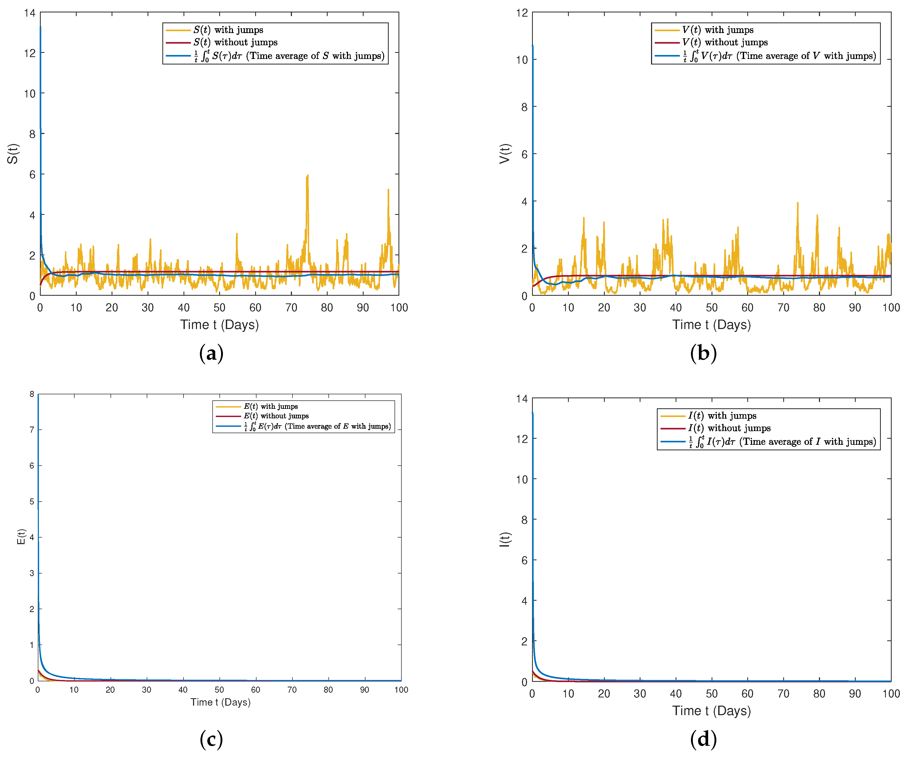
7. Numerical Results and Discussion

In this section, we present a graphical representation of the model dynamics using the available numerical method(s) and values of the parameters discussed in the previous section. For illustrative purposes, we provide the findings of our scheme and compute the approximate paths for the stochastic model (3) and its deterministic counterpart. The desired time interval is $[0,100]$ and the step size is $\Delta =0.3$, whereas the initial size of the population is provided by $({\mathbb{S}}_0,{\mathbb{V}}_0,{\mathbb{E}}_0,{\mathbb{I}}_0,{\mathbb{H}}_0,{\mathbb{R}}_0)=(0.5,0.4,0.3,0.5,0.2,0.1)$.

To simulate the model, we utilized two different types of hypothetical data. Initially, we simulated the model by considering the intensity of the noise and the parameter values from Example 1. The figure presented in Figure 3 demonstrates that as ${\mathrm{R}}_0^D<1$, the solution of system (3) with L’evy jump approaches the disease-free equilibrium point of the corresponding deterministic system, indicating that the disease is in the process of disappearing. Theorem 2 provides the necessary conditions for the extinction of system (3). The graphical representation verifies that the result of Theorem 2 is valid only if ${\mathbb{R}}_s<1$.

Example 1.

In the present scenario, we have considered the parameter values as $\varphi =1.0$, $\tau =0.3$, $\alpha =0.3$, $\mu =0.03$, $\beta =0.005$, $\delta =0.4$, $\gamma =0.02$, $\rho =0.01$, $\omega =0.02$, and the intensities of the white noise as ${\xi }_1=0.55$, ${\xi }_2=0.40$, ${\xi }_3=0.30$, ${\xi }_4=0.20$, ${\xi }_5=0.10$, ${\xi }_6=0.20$, and ${\mathbb{X}}_i\left(y\right)=\frac{-k_i{y}^2}{1+y^2}$, with $y=0.5$ and $k_i$ equal to $0.50$, $0.50$, $0.40$, $0.20$, $0.20$, and $0.30$, respectively, for $i=1,\cdots ,6$. The simulations of the model indicate that the epidemic will become extinct, as predicted by Theorem 2. The disappearance of the infection based on the predictions of the stochastic system are depicted in Figure 3a–f.

The findings of Theorem 3 suggest that the disease will continue to exist in the community with the dynamics predicted by model (3) if the value of ${\mathbf{R}}_{\mathbf{0}}^{\mathbf{D}}$ is greater than 1. The statement ${\mathbf{R}}_{\mathbf{0}}^{\mathbf{D}}>1$ indicates that ${\mathbf{R}}_{\mathbf{0}}^{\mathbf{s}}$ will be greater than 1 even with low intensities of the noise. This conclusion is supported by the numerical simulations presented in Figure 3c,d and Figure 4c,d, which validate the expected behavior of the epidemic model (3) as per Theorem 3.

Example 2.

In this example, the numerical values of the parameters are $\varphi =0.9$, $\tau =0.75$, $\alpha =0.5$, $\mu =0.06$, $\beta =0.05$, $\delta =0.4$, $\gamma =0.2$, $\rho =0.1$, and $\omega =0.2$, and the intensity of the white noise is ${\xi }_1=0.45$, ${\xi }_2=0.30$, ${\xi }_3=0.10$, ${\xi }_4=0.20$, ${\xi }_5=0.15$, ${\xi }_6=0.20$, and ${\mathbb{X}}_i\left(y\right)=\frac{-k_i{y}^2}{1+y^2}$, with $y=0.5$ and where $k_i$ equal to $0.50$, $0.35$, $0.30$, $0.35$, $0.10$, and $0.20$, respectively, for $i=1,\cdots ,6$.

For this set of parameters, it is easy to verify that both the stochastic threshold ${\mathbf{R}}_{\mathbf{0}}^{\mathbf{s}}$ and the basic reproduction number ${\mathbf{R}}_{\mathbf{0}}^{\mathbf{D}}$ are greater than one. The simulation results of the mean shown in Figure 4 confirm the persistence of the disease, which supports the conclusion of Theorem 3. Additionally, Figure 4a–f illustrates that the epidemic will continue to persist in the population in the meantime.

The Impact of Lévy Noise on the $\mathbb{I}$ Class

The impact of the intensity of the white noise on class $\mathbb{I}$ corresponding to system (3) is shown in Figure 5a–c. These figures suggest that increasing values of ${\xi }_i$ for $i=1,\cdots ,6$ lead towards the extinction of the disease. This means that the size of the infected class approaches zero as the intensity value of the noise increases. Further, this indicates that for small values of the noise intensity the infected class oscillates around the endemic steady state ${\mathbb{I}}^{★}$m which confirms the result of Theorem 3. However, if the intensity of the white noise term is sufficiently high, the solution $\mathbb{I}$ may not exhibit oscillations near the endemic equilibrium point. This demonstrates that continuous efforts to increase stochastic disruptions through mass recovery of susceptible individuals and the effective treatment and care of the infected persons can significantly lower the spread of the measles virus in the population.

8. Concluding Remarks and Future Directions

In this work, we have considered a stochastic $\mathbb{S}\mathbb{V}\mathbb{E}\mathbb{I}\mathbb{H}\mathbb{R}$ epidemic model with Lévy noise while considering the nonlinear incidence rate. Our study aimed to investigate the impact of environmental noise on human society, and the results can shed light on the crucial role of noise in disease persistence and extinction. The proposed model assumed six different classes: a healthy class $\left(\mathbb{S}\right)$, vaccinated class $\left(\mathbb{V}\right)$, infected class $\left(\mathbb{I}\right)$, exposed class $\left(\mathbb{E}\right)$, hospitalized class $\left(\mathbb{H}\right)$, and class of recovered individuals $\left(\mathbb{R}\right)$. After model formulation, the study utilized the uniqueness and existence techniques to derive a positive solution for the underlying stochastic model. The stability results of the model were investigated using the Lyapunov function. The model’s dynamic characteristics were analyzed in the context of the infection-free and endemic states of the associated ODE model. The stochastic threshold ${\mathbb{R}}_s$ was calculated to ensure disease extinction whenever ${\mathbb{R}}_s<1$. Using data from Pakistan in 2019, we estimated the model parameters and conducted simulations to forecast future disease behavior. The results were compared to actual data using standard curve fitting tools. In our future research, we plan to investigate the impact of regime switching and temporary immunity on system (3).

References

1. Mose, O.F.; Sigey, J.K.; Okello, J.A.; Okwoyo, J.M.; Giterere, J. Mathematical Modeling on the Control of Measles by Vaccination: Case Study of Kisii County, Kenya; Kenya Education Research Database: Kenya, 2014; Available online: https://kerd.ku.ac.ke/ (accessed on 16 April 2023).
2. Garba, S.M.; Safi, M.A.; Usaini, S. Mathematical model for assessing the impact of vaccination and treatment on measles transmission dynamics. Math. Methods Appl. Sci. 2017, 40, 6371–6388. [Google Scholar] [CrossRef]
3. Roberts, M.G.; Tobias, M.I. Predicting and preventing measles epidemic in New Zealand: Application of mathematical model. Epidem. Infect. 2000, 124, 279–287. [Google Scholar] [CrossRef] [PubMed]
4. Qureshi, S.; Jan, R. Modeling of measles epidemic with optimized fractional order under Caputo differential operator. Chaos Solitons Fractals 2021, 145, 110766. [Google Scholar] [CrossRef]
5. Perry, R.T.; Halsey, N.A. The clinical significance of measles: A review. J. Infect. Dis. 2004, 189 (Suppl. S1), S4–S16. [Google Scholar] [PubMed]
6. Guo, B.; Khan, A.; Din, A. Numerical Simulation of Nonlinear Stochastic Analysis for Measles Transmission: A Case Study of a Measles Epidemic in Pakistan. Fractal Fract. 2023, 7, 130. [Google Scholar] [CrossRef]
7. Mossong, J.; Muller, C.P. Modelling measles re-emergence as a result of waning of immunity in vaccinated populations. Vaccine 2003, 21, 4597–4603. [Google Scholar] [CrossRef] [PubMed]
8. Bolarin, G. On the dynamical analysis of a new model for measles infection. Int. J. Math. Trends Technol. 2014, 2, 144–155. [Google Scholar] [CrossRef]
9. Taiwo, L.; Idris, S.; Abubakar, A.; Nguku, P.; Nsubuga, P.; Gidado, S. Factors affecting access to information on routine immunization among mothers of under 5 children in Kaduna state Nigeria, 2015. Pan Afr. Med. J. 2017, 27, 1–8. [Google Scholar] [CrossRef] [PubMed]
10. Mere, M.O.; Goodson, J.L.; Chandio, A.K.; Rana, M.S.; Hasan, Q.; Teleb, N.; Alexander, J.P., Jr. Progress toward measles elimination—Pakistan, 2000–2018. Morb. Mortal. Wkly. Rep. 2019, 68, 505. [Google Scholar] [CrossRef] [PubMed]
11. World Health Organization. Eastern Mediterranean Vaccine Action Plan 2016–2020: A Framework for Implementation of the Global Vaccine Action Plan (No. WHO-EM/EPI/353/E); World Health Organization, Regional Office for the Eastern Mediterranean: Geneva, Switzerland, 2019.
12. Memon, Z.; Qureshi, S.; Memon, B.R. Mathematical analysis for a new nonlinear measles epidemiological system using real incidence data from Pakistan. Eur. Phys. J. Plus 2020, 135, 378. [Google Scholar] [CrossRef] [PubMed]
13. Din, A.; Ain, Q.T. Stochastic optimal control analysis of a mathematical model: Theory and application to non-singular kernels. Fractal Fract. 2022, 6, 279. [Google Scholar] [CrossRef]
14. Khan, F.M.; Khan, Z.U.; Lv, Y.P.; Yusuf, A.; Din, A. Investigating of fractional order dengue epidemic model with ABC operator. Results Phys. 2021, 24, 104075. [Google Scholar] [CrossRef]
15. Liu, P.; Ikram, R.; Khan, A.; Din, A. The measles epidemic model assessment under real statistics: An application of stochastic optimal control theory. Comput. Methods Biomech. Biomed. Eng. 2022, 26, 138–159. [Google Scholar] [CrossRef] [PubMed]
16. El Fatini, M.; Sekkak, I. Lévy noise impact on a stochastic delayed epidemic model with Crowly–Martin incidence and crowding effect. Phys. Stat. Mech. Its Appl. 2020, 541, 123315. [Google Scholar] [CrossRef]
17. Sabbar, Y.; Khan, A.; Din, A.; Tilioua, M. New Method to Investigate the Impact of Independent Quadratic Stable Poisson Jumps on the Dynamics of a Disease under Vaccination Strategy. Fractal Fract. 2023, 7, 226. [Google Scholar] [CrossRef]
18. Berrhazi, B.E.; El Fatini, M.; Caraballo Garrido, T.; Pettersson, R. A stochastic SIRI epidemic model with Lévy noise. Discret. Contin. Dyn.-Syst.-Ser. B 2018, 23, 3645–3661. [Google Scholar] [CrossRef]
19. Li, X.P.; Din, A.; Zeb, A.; Kumar, S.; Saeed, T. The impact of Lévy noise on a stochastic and fractal-fractional Atangana–Baleanu order hepatitis B model under real statistical data. Chaos Solitons Fractals 2022, 154, 111623. [Google Scholar] [CrossRef]
20. James Peter, O.; Ojo, M.M.; Viriyapong, R.; Abiodun Oguntolu, F. Mathematical model of measles transmission dynamics using real data from Nigeria. J. Differ. Equ. Appl. 2022, 28, 753–770. [Google Scholar] [CrossRef]
21. Zhao, Y.; Jiang, D. The threshold of a stochastic SIRS epidemic model with saturated incidence. Appl. Math. Lett. 2014, 34, 90–93. [Google Scholar] [CrossRef]
22. Zhao, Y.; Jiang, D. The threshold of a stochastic SIS epidemic model with vaccination. Appl. Math. Comput. 2014, 243, 718–727. [Google Scholar] [CrossRef]
Figure 1. Moments of individuals among the classes in the measles model (1) [21].
Fractalfract 07 00434 g001
Figure 2. Fitting of the model (1) against reported measles cases from Table 1.
Fractalfract 07 00434 g002
Figure 3. The plot shows the dynamics of the stochastic system (3) and the associated deterministic system (1) subject to jumps and without jumps. (a) The plot shows the S ( t ) —curve with and without jumps. (b) The plot shows the dynamics of V ( t ) with and without jumps. (c) Three different scenarios for class I ( t ) . (d) The dynamics of the exposed class with and without jumps. (e) Time evolution of the number of hospitalized people with and without jumps. (f) Three different scenarios for class R ( t ) .
Fractalfract 07 00434 g003aFractalfract 07 00434 g003b
Figure 4. Simulation of the stochastic system (3) and deterministic system (1) with and without jumps for the case when the respective thresholds are greater than one. (a) The dynamics of the susceptible class with and without jumps. (b) Time evolution of the number of vaccinated people both with and without jumps. (c) The plot shows the E ( t ) —curve with and without jumps. (d) The dynamics of the infected class with and without jumps. (e) The plot shows the H ( t ) —curve with and without jumps. (f) Time evolution of the number of recovered people when the threshold exceeds one.
Fractalfract 07 00434 g004aFractalfract 07 00434 g004b
Figure 5. Simulations of I ( t ) based on the stochastic and deterministic systems, showing the effect of the intensities on class I when ϕ = 0.5 , τ = 0.90 , α = 0.5 , μ = 0.06 , β = 0.05 , δ = 0.4 , γ = 0.2 , ρ = 0.2 , ω = 0.3 , and the noise intensity is assumed as ξ 1 = 0.50 , ξ 2 = 0.40 , ξ 3 = 0.10 , ξ 4 = 0.20 , ξ 5 = 0.15 , ξ 6 = 0.20 , and X i ( y ) = k i y 2 1 + y 2 , with y = 0.5 and where k i equals 0.60 , 0.34 , 0.30 , 0.35 , 0.10 , 0.20 , respectively, for i = 1 , , 6 and ( S 0 , V 0 , E 0 , I 0 , H 0 , R 0 ) = ( 0.5 , 0.4 , 0.5 , 0.3 , 0.2 , 0.1 ) . (a) The dynamics of I ( t ) subject to sufficiently large values of noise intensity. (b) The plot shows the behavior of the infected class subject to moderate values of noise intensity. (c) The dynamic behavior of the infected class subject to low values of noise intensity.
Fractalfract 07 00434 g005