Article

A Novel Grey Seasonal Model for Natural Gas Production Forecasting

School of Mathematical Sciences, Henan Institute of Science and Technology, Xinxiang 453003, China
*
Author to whom correspondence should be addressed.
Fractal Fract. 2023, 7(6), 422; https://doi.org/10.3390/fractalfract7060422
Submission received: 5 March 2023 / Revised: 15 May 2023 / Accepted: 17 May 2023 / Published: 24 May 2023

Abstract

:
To accurately predict the time series of energy data, an optimized Hausdorff fractional grey seasonal model was proposed based on the complex characteristics of seasonal fluctuations and local random oscillations of seasonal energy data. This paper used a new seasonal index to eliminate the seasonal variation of the data and weaken the local random fluctuations. Furthermore, the Hausdorff fractional accumulation operator was introduced into the traditional grey prediction model to improve the weight of new information, and the particle swarm optimization algorithm was used to find the nonlinear parameters of the model. In order to verify the reliability of the new model in energy forecasting, the new model was applied to two different energy types, hydropower and wind power. The experimental results indicated that the model can effectively predict quarterly time series of energy data. Based on this, we used China’s quarterly natural gas production data from 2015 to 2021 as samples to forecast those for 2022–2024. In addition, we also compared the proposed model with the traditional statistical models and the grey seasonal models. The comparison results showed that the new model had obvious advantages in predicting quarterly data of natural gas production, and the accurate prediction results can provide a reference for natural gas resource allocation.

1. Introduction

1.1. Background

With the rapid development of human society and the increasing energy demand, the extensive consumption of fossil energy has brought excessive greenhouse gas emissions and environmental pollution. Therefore, an energy revolution is needed to fundamentally change the energy consumption mode of society and realize sustainable development. Building a clean, low-carbon, safe, and efficient energy system has become the consensus and development direction of the global oil and gas industry. Compared with coal and oil, natural gas has the advantages of a wide range of uses, safety and convenience, high calorific value, clean environmental protection, and so on. In the “14th Five-Year Plan” energy plan, China pointed out that it is necessary to focus on improving the reserves and supply capacity of natural gas. Persisting on increasing natural gas production and actively expanding the exploration and development of unconventional resources are the main goals of the natural gas industry. However, China’s natural gas market is still in the cultivation stage. Efforts to expand consumption and the natural gas industry are indispensable parts of China’s energy transformation. In recent years, China’s natural gas consumption has entered a period of rapid development. Its rapid growth has also led to the continuous expansion of domestic production and import scale. Natural gas production and consumption in China from 2015 to 2021 are shown in Figure 1. From this, we can see that the output growth rate is slow while the consumption growth is too fast, and the gap between production and demand in China is increasing yearly. In order to balance supply and demand, China’s natural gas imports reached 202.23 million tons of coal equivalent in 2021, an increase of 13.86% compared to the previous year. In the case of China’s high dependence on foreign natural gas, how to effectively meet the growth of China’s natural gas demand in the future is the focus of many scholars’ research.

1.2. Research Progress in Natural Gas Forecasting

So far, scholars’ research on natural gas has mainly focused on predicting consumption and production. The commonly used prediction methods for natural gas can be divided into three categories: economic statistics, grey model, and intelligent algorithm. The statistical method used is mainly time series analysis, which is widely used in energy prediction. Example: Non-residential natural gas consumption in Italy was predicted by using a regression model [1]. A structured time series model (STSM) was used to forecast natural gas demand in Europe [2]. However, the statistical model requires long-term data accumulation and cannot reflect the attenuation of the contribution rate of some distinguishing factors over time.
Grey system theory, which can quantify uncertain factors, is often used to build medium and short-term natural gas prediction models. Examples are as follows: A nonlinear grey Bernoulli model (WFNGBM (1,1, N)) was built to predict China’s natural gas production [3]. A fractional-order incomplete gamma grey model was established to predict natural gas consumption in the Asia Pacific region from 2008 to 2018 [4]. A new grey metabolic GM (1,1) model is proposed, which is based on the latest data generated by the system and replaces the oldest data in the original sequence one by one to improve prediction accuracy [5]. Aiming at the disadvantage of “dislocation replacement” in the transformation process of the traditional grey model from difference equation to differential equation, a new unbiased grey prediction model UGM (1,1) was proposed for forecasting the output of shale gas in China [6]. However, the conventional grey model prediction results often have some shortcomings. To solve this problem, some scholars have put forward some new methods. The details are as follows: The log equation necessary form of the generalized Weng’s model was introduced into the grey model, which improves the model’s adaptability and forecasts China’s natural gas production from 2012 to 2025 [7]. To forecast China’s use of natural gas, a polynomial grey model with time delay (TDPGM (1,1)) was presented [8]. Zheng et al. proposed the conformable fractional non-homogeneous grey Bernoulli model, which was abbreviated as CFNHGBM (1,1,k), and predicted the production and consumption of natural gas in North America from 2008 to 2018 [9]. Based on the traditional GM (1,1) model, Ye et al. established a grey residual GM (1,1) model and predicted natural gas consumption in China. By comparing the prediction accuracy of the residual GM (1,1) model and the traditional GM (1,1) model, it was found that the residual GM (1,1) model further improved the prediction accuracy and was suitable for natural gas consumption prediction research [10]. In practical application, the single prediction model is often challenging to realize the natural gas demand prediction of multi-dimensional influencing factors. The combined prediction model can maximize the unique advantages of the single prediction model, enhance its strengths and avoid weaknesses, and improve the accuracy of prediction results. A grey neural network and input-output combined prediction model were proposed, which fully considers the potential complex nonlinear relationship and effectively improves the prediction accuracy [11]. To more accurately estimate China’s real natural gas consumption, a novel combined prediction model was established by utilizing the optimized grey Verhulst model and the nonlinear grey Bernoulli model [12].
In recent years, to solve the nonlinear decision-making problem, some scholars have successively used intelligent algorithms such as neural networks and genetic algorithms to build natural gas prediction models. For example, a grey-related least squares support vector machine model was constructed. The second-order particle swarm optimization algorithms (SecPSO) were used to optimize the model parameters to predict China’s annual natural gas consumption [13]. Based on the Ant Lion Optimization algorithm (ALO), an adaptive grey prediction system with nonlinear optimization initial value was proposed [14]. An artificial bee colony (ABC) algorithm was designed to solve the continuous optimization problem, and the natural gas consumption of Turkey from 2018 to 2030 is predicted [15]. To forecast the short-term consumption of natural gas, a new hybrid prediction model is established by combining Volterra adaptive filtering with an improved whale optimization algorithm [16].

1.3. Application of Grey Season Model in Natural Gas

From the quarterly perspective of the data, China’s natural gas production has apparent seasonal and cyclical fluctuations. As shown in Figure 2, from the first quarter of 2015 to the fourth quarter of 2021, natural gas production in the first and fourth quarters is significantly higher than that in the second and third quarters. It is greatly influenced by the consumption market and has prominent seasonal characteristics. The conventional GM (1,1) model can reflect the general trend of time series. However, it cannot accurately reflect the distinct characteristics of seasonal variation and has obvious limitations in the simulation and prediction of seasonal time series. Therefore, the methods of applying grey system theory to deal with seasonal data are mainly divided into two aspects. The first aspect primarily focuses on data preprocessing to eliminate the seasonal fluctuation characteristics of the original series and create a suitable modeling environment. Examples include the following: To capture seasonality, the seasonal index was constructed by using the average method of the same period, and the original data were preprocessed. The proposed fractional seasonal grey model also described the seasonal fluctuation characteristics well [17]. Through favorable translation and weighted geometric mean transformation, the smoothness of the sequence was gradually improved, the grey exponential law was apparent, and the prediction accuracy of the model is improved [18]. A grey modeling method DGGM (1,1), based on data grouping, was proposed to predict the quarterly time series [19]. The enhanced and weakened buffer operators were used to improve the smoothness of the original sequence, create the conditions in line with grey modeling, and then solve the problem of prediction modeling [20]. A dynamic seasonal index was constructed to improve the data preprocessing method of the single seasonal index, which was more representative than the single seasonal index, and improves the quality of the input data of the model after preprocessing [21].
On the other hand, the method to deal with seasonal data is to study the adaptive improvement of the model. The combined model is created to make the prediction model more suitable for seasonal forecast data without changing the trend of the original data. By adding an adaptive parameter learning mechanism to the fractional seasonal grey model (SFGM (1,1)), a combined forecasting model called the adaptive seasonal grey model (APL-SFGM (1,1)) is established to improve the forecasting ability of the model [22]. Zeng et al. used the interval grey number modeling method to simulate and predict the range of oscillation sequence values, and this method is used to simulate the variation law of the Chongqing air quality index (AQI) with oscillation characteristics [23]. In order to solve the problem of inaccurate prediction caused by large fluctuations of original data and improve the accuracy of prediction results, a combined optimization approach of k-nearest neighbor and particle swarm optimization was developed to predict monthly electricity consumption [24]. In addition, the data with seasonal changes also belong to oscillation data. For oscillatory data, some scholars have introduced the concept of the power model. Because the power model has the advantage of strong adaptability to the original data, it accounts for a large proportion of the adaptive improvement of the model. Examples include the following: For a small sample oscillation sequence, an oscillation GM (1,1) power model with system delay and time-varying parameters was proposed. The nonlinear optimization model was constructed to find the best power exponent and time action parameters and to identify the oscillation characteristics contained in the original data [25]. Based on the GM (1,1) power model, the periodic oscillation law of the residual sequence was proposed by using the Fourier series, and a prediction model suitable for small sample oscillation series is established [26]. According to the oscillation characteristics of the original series, the value of the power index is adjusted flexibly. That is to say, the shape of the prediction curve is changed to make the model achieve higher prediction accuracy, and the GM (1,1|sin) model is established [27]. When predicting some seasonal data, some scholars are concerned that the original data may have a dual trend of growth and seasonal fluctuation. Given this perspective, the literature [28] established a comprehensive optimal prediction model combined with the respective characteristics of the grey prediction model and support vector machine prediction model. It used the improved particle swarm optimization algorithm to solve the weight of the combined prediction model. Reference [29] proposed to combine the grey prediction method with the seasonal variation index to solve the complex uncertainty problem and established the dynamic Seasonal Model (GSVI (1,1)), which enhanced the adaptability of the grey model. Reference [30] proposed a fractional order cumulative particle swarm optimization grey seasonal model (PSO-FGSM (1,1) model) emphasizing the principle of new information priority. On this basis, the reference [31,32,33] introduces the Hausdorff fractional grey model, which further improves the prediction accuracy and stability of the model. Similarly, the sample data of natural gas production in China has a dual trend of growth and seasonal fluctuation. Based on previous studies, this paper adopts the moving average method in the time series analysis method to eliminate the seasonal influence in the periodic oscillation series, constructs a new seasonal index, and introduces the idea of seasonal index into the Hausdorff fractional grey seasonal model. Then the particle swarm optimization algorithm (PSO) is used to find the nonlinear parameters of the model.

1.4. Aim, Contribution, and Organization

According to the above research, China’s continued expansion in natural gas production will not only affect international natural gas commerce in recent years but also have a more far-reaching impact on the global natural gas pattern. Improving the accuracy of China’s quarterly natural gas data forecasts can assist and clarify future supply scenarios. Optimizing the allocation of social resources according to forecasts is also conducive to taking practical measures in advance to ensure healthy and rapid economic development. Based on the literature review of grey model forecasting of natural gas in China and some seasonal improvement methods summarized above, the main contributions of this paper are as follows.
The first contribution of this paper is to pay attention to the seasonal and periodic fluctuation characteristics of China’s natural gas production and construct the seasonal index by using the quadratic moving average method. Through preprocessing the original data, the seasonal and periodic fluctuation characteristics of the data are eliminated. At present, scholars’ research on natural gas is mainly focused on annual forecasts, but there is not much research on the quarterly forecast. Considering the use of quarterly data to predict natural gas production is helpful for the country to realize the medium-and short-term regulation and control plan of natural gas.
The second contribution of this paper is to introduce the Hausdorff fractional order accumulating operator into the grey season model, and adjust the weight of information by changing the order of the incremental generation operator so that new information has more priority in the model. The novel model further improves the practical value of the model, realizes high-precision prediction and analysis of natural gas production, and reveals the evolution law of natural gas production.
The rest of this paper is organized as follows: The methods and specific models used in this study are described in Section 2. Section 3 conducted testing and analysis on examples outside of the sample. Quarterly natural gas production in China is predicted in Section 4. Section 5 offers conclusions and prospects.

2. Methodology

2.1. The Traditional FHGM (1,1) Model [33]

Definition 1.
Assume  X ( 0 ) = ( x ( 0 ) ( 1 ) , x ( 0 ) ( 2 ) , , x ( 0 ) ( n ) )  is a non-negative sequence, and then its r-order accumulative sequence is given by  X ( r ) = ( x ( r ) ( 1 ) , x ( r ) ( 2 ) , , x ( r ) ( n ) ) , then the differential equation of the FHGM (1,1) model is
d x ( r ) ( t ) d t + a x ( r ) ( t ) = b
where  x ( r ) ( k ) = i = 1 k x ( 0 ) ( i ) [ i r ( i 1 ) r ] ( k = 1 , 2 , , n ) .
Definition 2.
The basic form of the FHGM (1,1) model is
x ( r ) ( k ) x ( r ) ( k 1 ) + a z ( r ) ( k ) = b
where  z ( r ) ( k ) = x ( r ) ( k ) + x ( r ) ( k 1 ) 2 , k = 2 , 3 , , n .
Theorem 1.
Let  X ( 0 ) , X ( r )  are defined in Definition 1, the parameters  a b  of the FHGM (1,1) model can be estimated by the least square method, namely,
μ ^ = [ a , b ] T = ( B T B ) 1 B T Y
 where  B = 0.5 ( x ( r ) ( 1 ) + x ( r ) ( 2 ) ) 0.5 ( x ( r ) ( 2 ) + x ( r ) ( 3 ) ) 0.5 ( x ( r ) ( n 1 ) + x ( r ) ( n ) ) 1 1 1 ( n 1 ) × 2 , Y = x ( r ) ( 2 ) x ( r ) ( 1 ) x ( r ) ( 3 ) x ( r ) ( 2 ) x ( r ) ( n ) x ( r ) ( n 1 ) ( n 1 ) × 1
Theorem 2.
The initial value is  x ^ ( r ) ( 1 ) = x ( r ) ( 1 ) = x ( 0 ) ( 1 ) , then the time response function of the FHGM (1,1) model is
x ^ ( r ) ( k ) = ( x ( 0 ) ( 1 ) b a ) e a ( k 1 ) + b a
The restored values are  x ^ ( 0 ) ( k ) = x ^ ( r ) ( k ) x ^ ( r ) ( k 1 ) k r ( k 1 ) r k = 2 , 3 , , n .

2.2. The SFHGM (1,1) Model

The moving average model is a simple smooth forecasting technique and a common tool for processing seasonal time series data. The basic idea is to average the data of two or more periods of the original time series and replace the actual series value with the average value to smooth the periodicity.
Definition 3.
Suppose that  X = x 1 , x 2 , , x k  is a raw series influenced by season, the calculation formula of the first moving average is
M t 1 = x t m + 1 + x t m + 2 + + x t m ( t = m , m + 1 , , k )
where  m ( m k )  is the number of terms in the first moving average.
Similarly, the average calculation formula of the second movement is
M t 2 = M t N + 1 1 + M t N + 2 1 + + M t 1 N ( t = m + 1 , m + 2 , , k )
N ( N k m + 1 ) is the number of terms in the second moving average. Reference [34] used the Monte Carlo method to explore the relationship between the two moving average step sizes, and used the formula of mean square error to find the optimal moving step sizes. The results indicate that taking the asynchronous length of the second moving average is more accurate in predicting accuracy.
D is a series operator such that
X d r = X 0 D = x d r 1 , x d r 2 , , x d r k
with
x d r k = i = 1 k ( x 0 ( i ) / f d ( i ) ) ( [ i r ( i 1 ) r ] ) , k = 1 , 2 , , n .
f d ( i ) is the seasonal index acting on the i time point of the original series. D is the fractional-order seasonal cumulative generating operator. Seasonal index f d ( i ) is a dimensionless parameter, reflecting the average degree of deviation of the actual value from trend value due to seasonal influence in the current period. The calculation formula is as follows:
φ m j + i = x t M t 2 ( t = m + 1 , m + 2 , , k )
f d ( i ) = φ ¯ m j + i j = 1 , 2 , , k m N + 2 m , i = 1 , 2 , , m
f d ( i ) represents the average value of φ m j + i . It is noteworthy that if f d ( i ) = 1 for arbitrary i , then the seasonal cumulative generation operator is the same as the classical cumulative generation operator. The seasonal cumulative generating operator can be regarded as the extension and expansion of the classical cumulative generating operator.
On this basis, the background value Z d r ( k ) is generated for r order cumulative sequence. The formula is the following.
Z d r ( k ) = 0.5 x d r ( k ) + 0.5 x d r ( k 1 ) ,   k = 2 , 3 , , n
The grey difference equation is established as the following.
x d r k x d r k 1 + a s z d r k = b s
The corresponding whitening differential equation is the following:
d x d r ( t ) d t + a s x d r ( t ) = b s
where a s is the development coefficient, and b s is the grey action.
The parameter vector γ ^ s can be estimated by using the following formula:
γ ^ s = ( a s , b s ) T = ( B s T B s ) 1 B s T Y s
where
B s = z d r ( 2 ) z d r ( 3 ) 1 1 z d r ( n ) 1 ( n 1 ) × 2 , Y s = x d r 2 x d r 1 x d r 3 x d r 2 x d r n x d r n 1 ( n 1 ) × 1
The time response function can be obtained as
x ^ d r ( k ) = ( x 0 ( 1 ) / f d ( 1 ) b s a s ) e a s ( k 1 ) + b s a s , k = 2 , 3 , , n
The restored values can be obtained by the following formula x ^ d ( 0 ) ( k ) = x ^ d ( r ) ( k ) x ^ d ( r ) ( k 1 ) k r ( k 1 ) r , k = 2 , 3 , , n .
The Simulated value of original data obtained by seasonal index is x ^ 0 k = x ^ d 0 k × f d i .
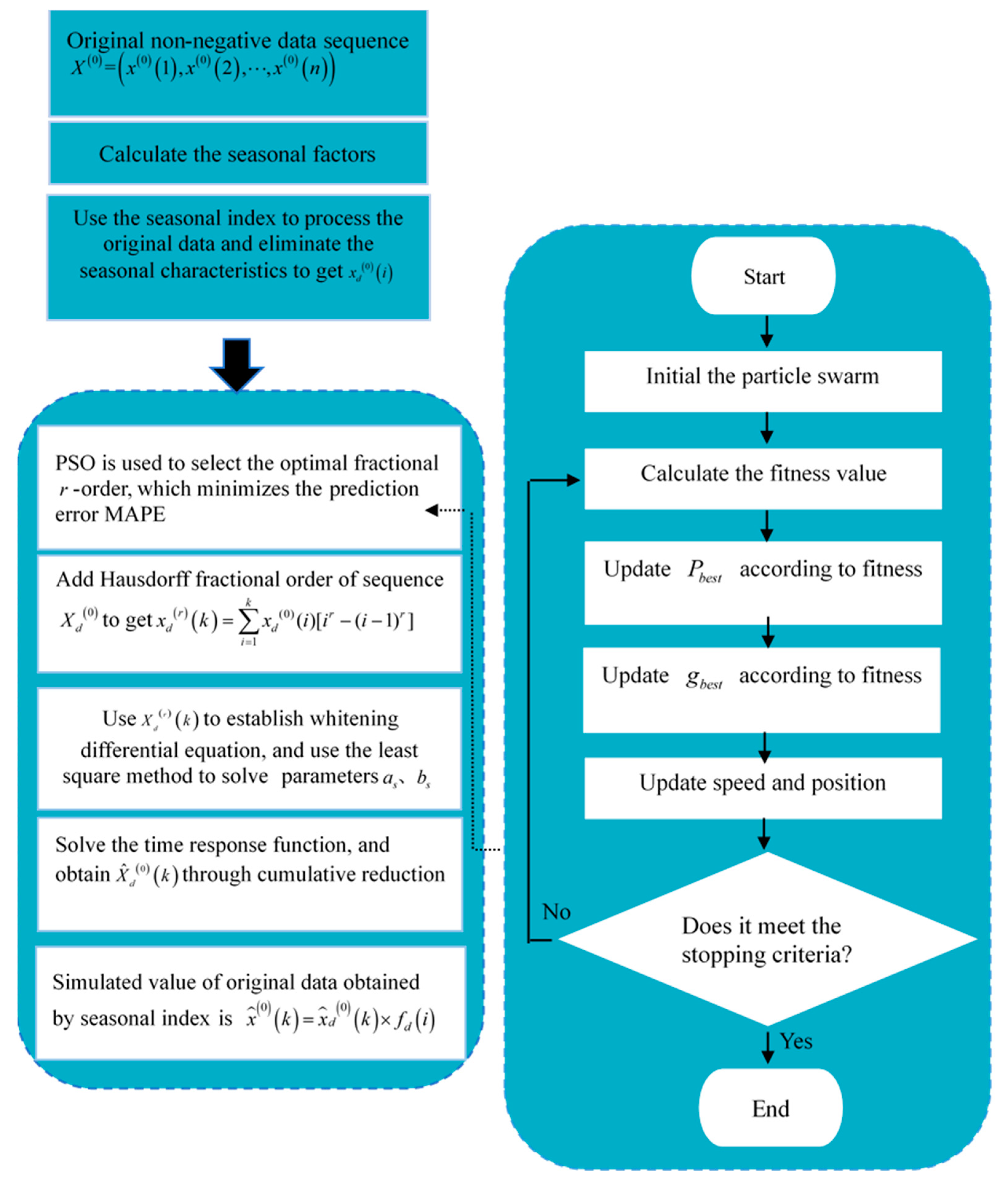
The steps involved in the modeling process can be illustrated using a flow chart (Figure 3).

2.3. Model Error Test Criteria

To ensure the high accuracy of the proposed model, some criteria are selected to test the model. They are absolute percentage error ( A P E ), the mean absolute error ( M A E ), mean absolute percentage error ( M A P E ), and root mean squared error ( R M S E ). The corresponding calculation formula is as follows:
A P E = x ^ 0 ( k ) x 0 ( k ) x 0 ( k ) × 100 %
M A E = 1 n k = 1 n x ^ 0 ( k ) x 0 ( k )
M A P E = 1 n k = 1 n x ^ 0 ( k ) x 0 ( k ) x 0 ( k ) × 100 %
R M S E = 1 n 1 k = 2 n x ^ 0 ( k ) x 0 ( k ) 2
where x ^ 0 ( k ) and x 0 ( k ) represent the predicted value and the corresponding actual value, respectively. The M A P E evaluation criteria are shown in Table 1.

3. Validation of the SFHGM (1,1) Model

In order to verify the applicability of the model, a series with seasonal fluctuations is randomly selected for numerical experiments. This section compares two numerical cases with other relevant prediction models. The test results show that the new model has good prediction performance.

3.1. Case 1. Forecasting Quarterly Hydropower Production in China

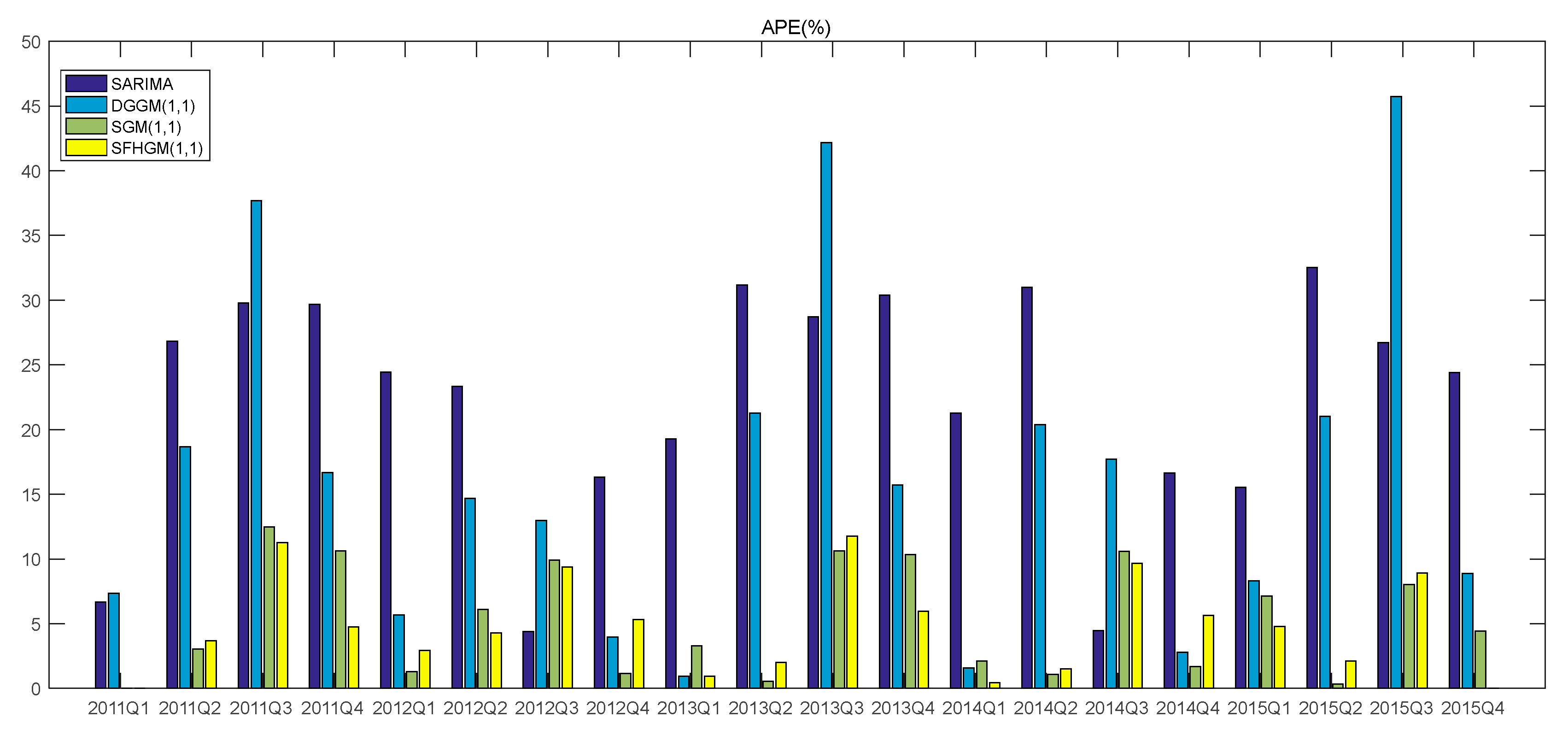
We consider an example from the paper [19], which provides the modeling data to build the grey models. As shown in Table 2, this paper takes the quarterly data of Hydropower output in China from 2011 to 2015 as the modeling sequence, and then tests the superiority of the model proposed in this paper by comparing three common seasonal models. The fitting effects of the four models were further analyzed with four error test standards. The results showed that the MAE, RMSE, and MAPE of the new model were 10.93%, 15.53%, and 4.8%, respectively, which are much lower than the other three models, as shown in Table 3 and Figure 4a. It can also be seen from Figure 4b and Figure 5 that the fitting curve of the new model is closer to the real value, and the prediction accuracy of each point is relatively stable, indicating that the new model has better applicability to deal with seasonal data.

3.2. Case 2 Forecasting Quarterly Wind Power Production in China

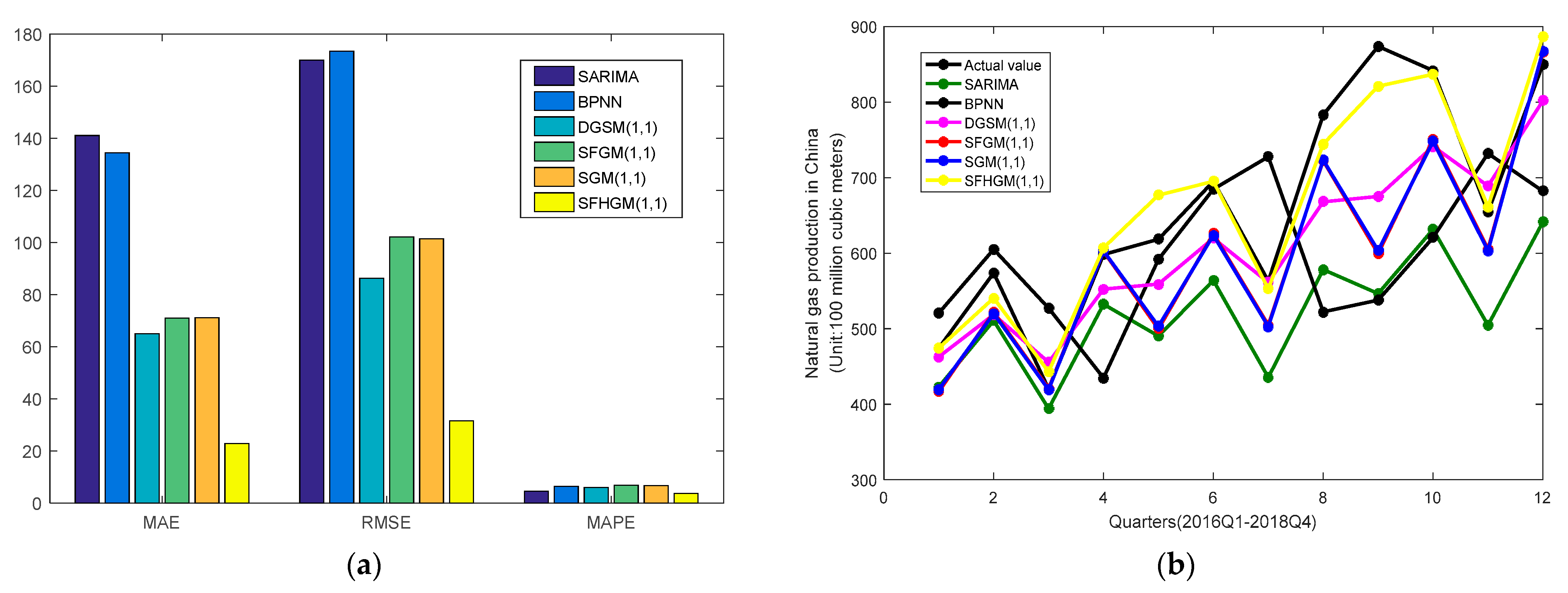
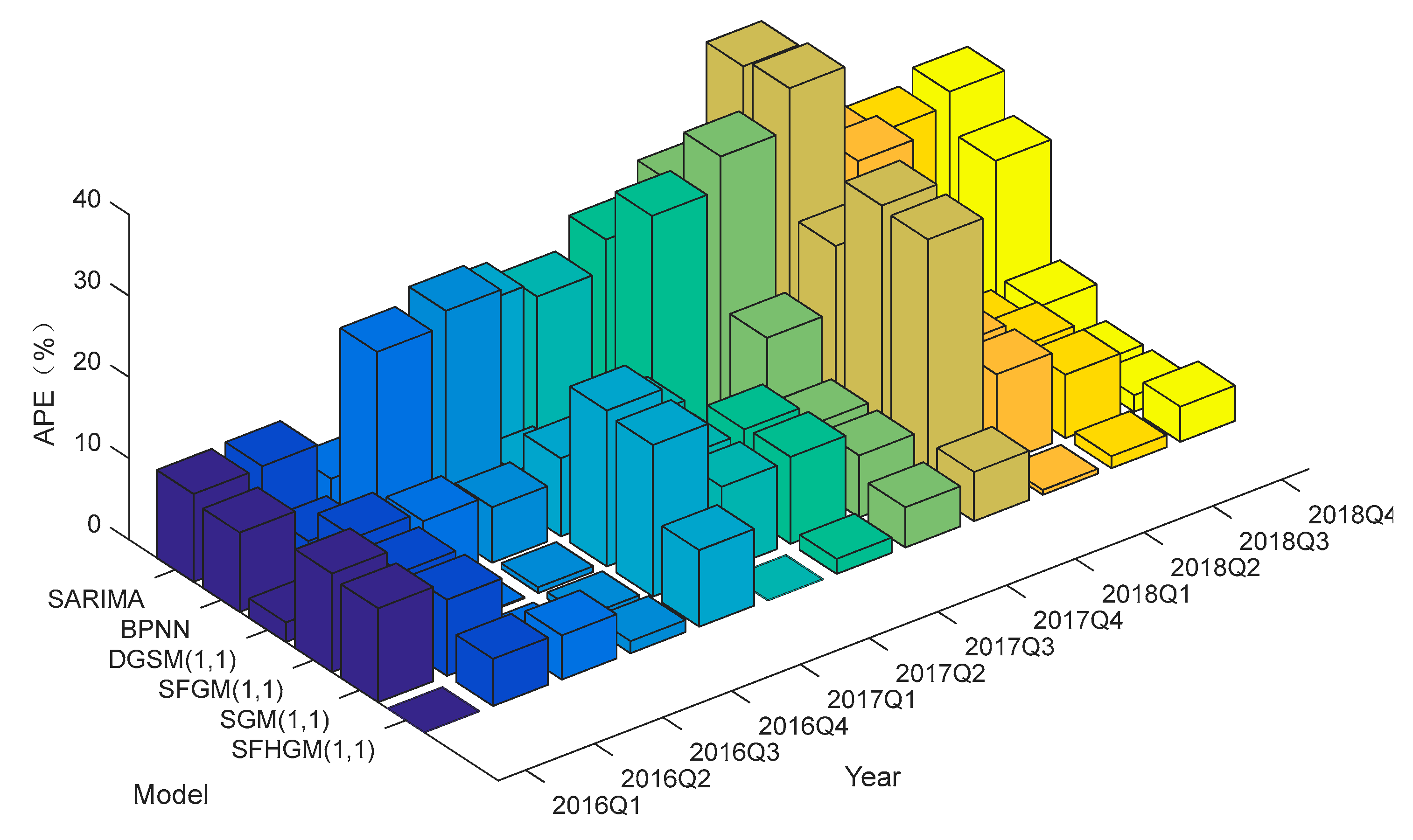
We consider an example from the paper [36], which provides the modelling data to build the grey models. As shown in Table 4, this paper uses the quarterly data of wind power output in China from 2016 to 2018 as the modeling sequence and then tests the superiority of the model proposed in this paper by comparing five common seasonal models. The fitting effects of the six models were further analyzed with four error test standards. The results showed that MAE, RMSE and MAPE of the new model were 22.84%, 31.53%, and 3.73%, all much lower than those of the other five models, as shown in Table 5 and Figure 6a. It can be seen from Figure 6b and Figure 7 that the new model adopted in this paper is superior to the model adopted by Ding et al. [14]. It can eliminate the influence of seasonal data, smooth the fluctuation of data, and improve the smoothness of the series, so as to achieve good prediction accuracy. It is also more stable and reliable in practical application.

4. Application

4.1. Data Description

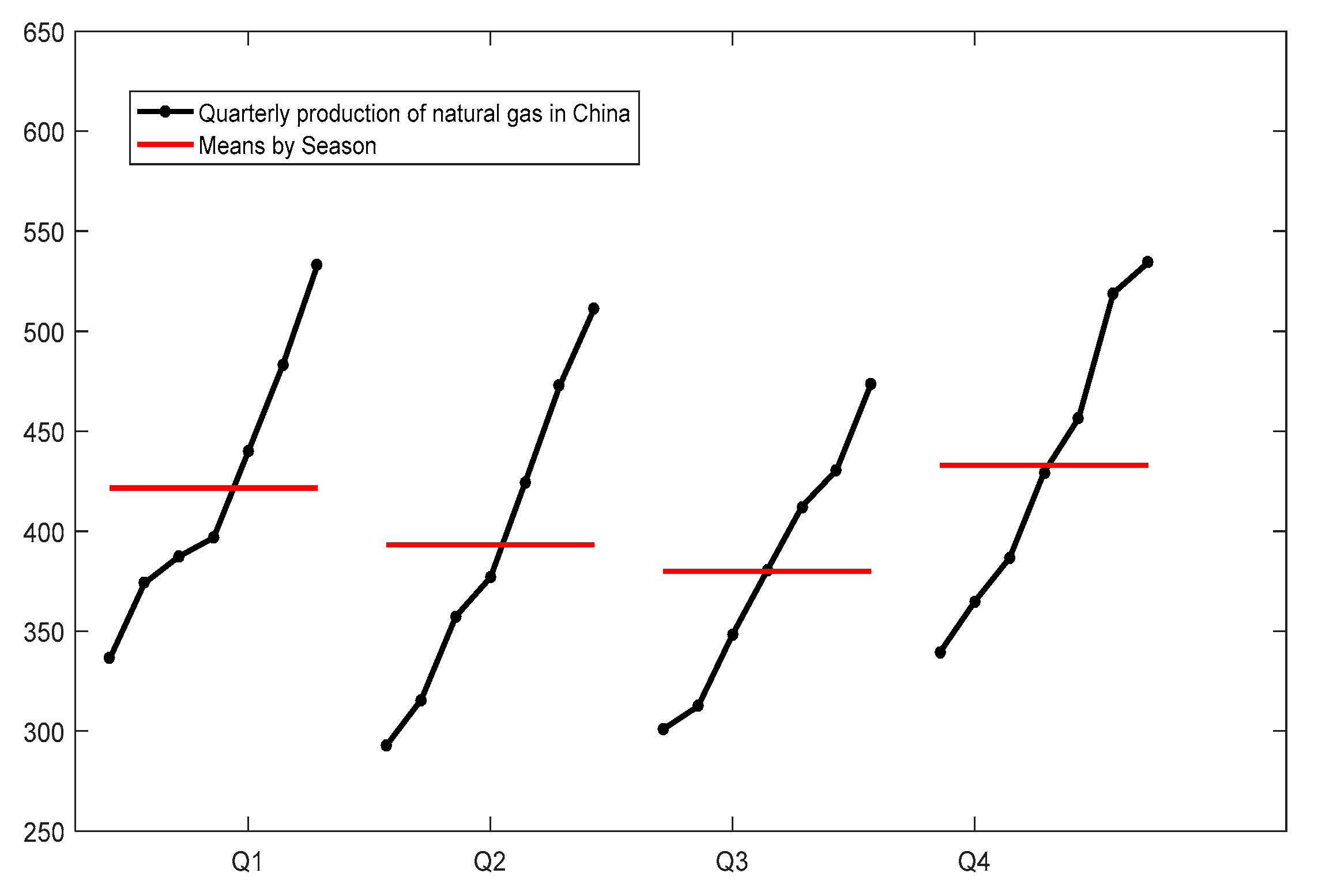
The quarterly data of China’s natural gas production from 2015 to 2021 are divided into four groups by season: Q1 (first quarter), Q2 (second quarter), Q3 (third quarter), and Q4 (fourth quarter) in winter. After grouping, it is found that natural gas production is the highest in winter and the lowest in autumn. The seasonal mean value of natural gas production is Q4 > Q1 > Q2 > Q3, as shown in Figure 8. The weather is cold in spring and winter, and there is a great demand for heating. As one of the main ways of heating, the consumption of gas heating increases sharply, so the output increases. The demand for heating is less in summer and autumn, the consumption of natural gas is relatively weaker, and the output will also be reduced. In recent years, with the implementation of the policy of replacing coal with gas, the consumption level and supply capacity of natural gas has been relatively improved, and the overall output has shown an upward trend.

4.2. Model Establishment

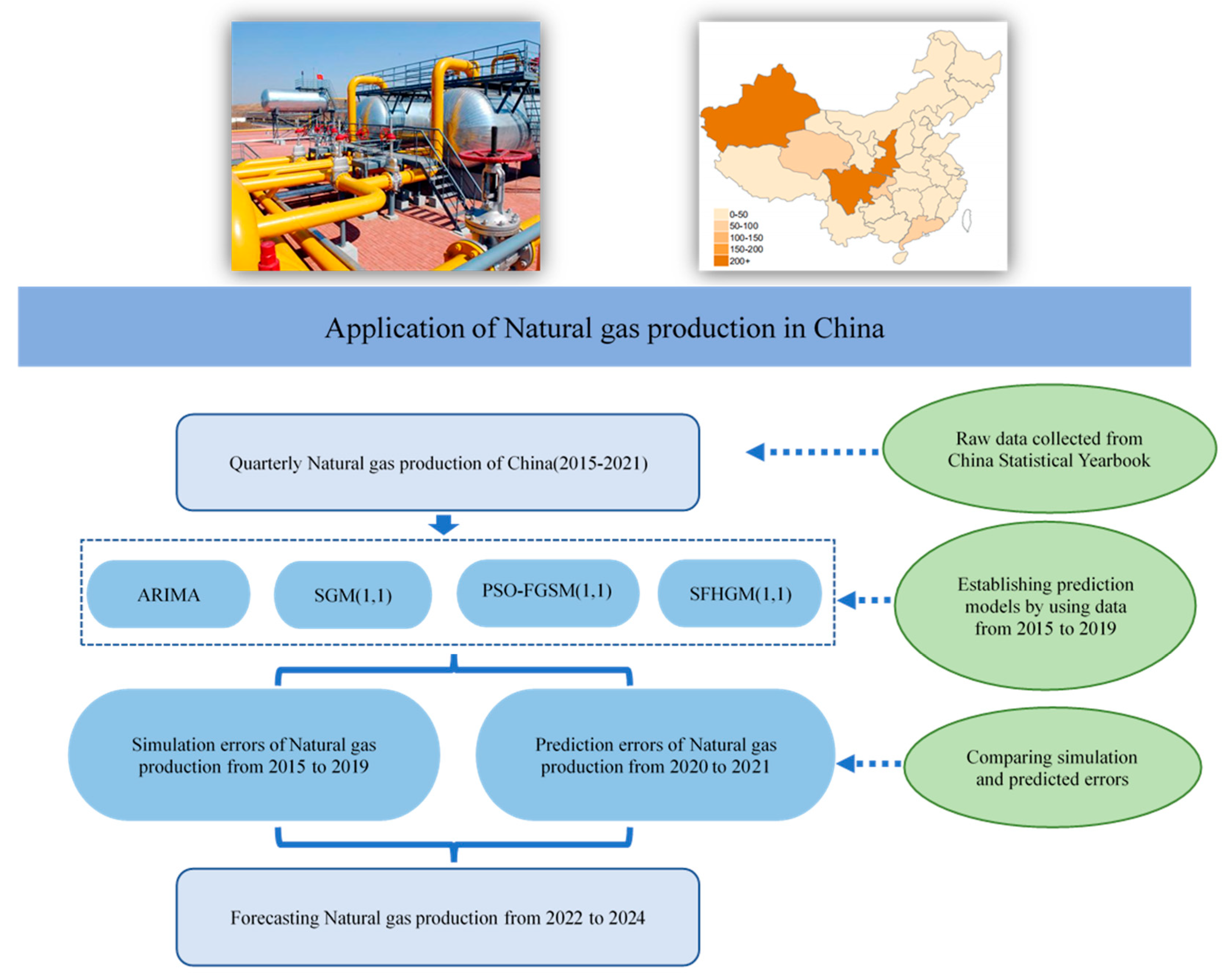
In this paper, the statistical model ARIMA, grey season model SGM (1,1), PSO-FGSM (1,1), and SFHGM (1,1) are compared and analyzed to verify the effectiveness and practicality of the new model. In the modeling process, the quarterly natural gas production data from 2015 to 2019 are used for simulation, and the data from 2020 to 2021 are used to verify the prediction effect. The structural chart of this study is graphed in Figure 9. From Figure 9, it can be seen that the quarterly production data of natural gas in China from 2015 to 2021 is sourced from the China Statistical Yearbook. Establish the ARIMA model, SGM (1,1) model, PSO-FSGM (1,1) model, and SFHGM (1,1) model using data from 2015 to 2019. Afterward, use each model to predict China’s quarterly natural gas production from 2020 to 2021. Calculate the estimation error for 2015–2019 and the prediction error for 2020–2021 based on quarterly natural gas data obtained from five models. Then, the estimation and prediction errors of the five models are compared to obtain a model with good estimation and prediction effects, which is used to predict the quarterly natural gas production in China from 2022 to 2024.

4.3. The Solution of SFHGM (1,1) Model

It can be known from Xi et al. [34] that when the sample size is greater than or equal to 20, the optimal step size of the two moving averages is not statistically independent, and the first moving average takes a larger value, while the second moving average takes a smaller value. Because the oscillation period of the original sequence was four and the sample size was 20, so m = 4 and N = 2 were selected. China’s natural gas production from 2015 to 2019 is selected for modeling calculations. The specific calculation process is as follows:
Firstly, according to Formula (4), we calculate the value after the first moving average with the following formulas.
M 4 ( 1 ) = 1 4 ( x 1 + x 2 + x 3 + x 4 ) = 317.5 ,   M 5 ( 1 ) = 1 4 ( x 2 + x 3 + x 4 + x 5 ) = 326.9
M 6 ( 1 ) = 332.6 , ,   M 20 ( 1 ) = 433.2
Similarly, the second moving average is processed on this basis, and the result is
M t 2 = M t N + 1 1 + M t N + 2 1 + + M t 1 N ,   M 5 ( 2 ) = ( M 5 ( 1 ) + M 4 ( 1 ) ) 2 = 322.2
M 6 ( 2 ) = 329.8 , , M 20 ( 2 ) = 429.8
Secondly, the weights of quarterly influencing factors were calculated according to Formulas 7 and 8, and the results are shown in Table 6. It can be seen that the seasonal deviation of the first quarter and the fourth quarter is significantly higher than that of the second quarter and the third quarter. This is because the production activities of natural gas are obviously affected by seasons and the production will also increase significantly. The detailed calculation process is as follows.
φ m j + i = x t M t ( 2 ) ( t = m + 1 , m + 2 , , k )
φ 5 = x 5 M 5 ( 2 ) = 1.16068 ,   φ 9 = x 9 M 9 ( 2 ) = 1.128048 ,   φ 13 = x 13 M 13 ( 2 ) = 1.06902 ,   φ 17 = x 17 M 17 ( 2 ) = 1.096109
φ i ( i = 4 , 6 , 7 , 8 , 10 , 11 , 12 , 14 , 15 , 16 , 18 , 19 , 20 ) can be obtained in the same way.
According to the following formula, we can calculate the seasonal index f d ( i )
f d ( i ) = φ ¯ m j + i j = 1 , 2 , , k m N + 2 m , i = 1 , 2 , , m
f d ( 1 ) = ( φ 5 + φ 9 + φ 13 + φ 17 ) 4 = 1.113464 , f d ( 2 ) = ( φ 6 + φ 10 + φ 14 + φ 18 ) 4 = 1.002941
Similarly, it can be concluded that f d ( 3 ) = 0.969268 , f d ( 4 ) = 1.073026 .
Thirdly, the original data are preprocessed with a seasonal index to eliminate its seasonal fluctuation characteristics, and then the SFHGM (1,1) model is constructed. The particle swarm optimization algorithm is used to solve each parameter of the SFHGM (1,1) model, and the results are shown in Table 7.
Lastly, the restoration value can be calculated by multiplying the predicted value by the relevant seasonal index. The fitting and prediction results are shown in Table 8. The SFHGM (1,1) model also forecasts China’s quarterly natural gas production from 2022 to 2024, the predicted results are shown in Table 9.

4.4. Model Comparison

The left side of the vertical dotted line in Figure 10 shows the fitting effects of the four models, and the right side shows the prediction effects of the four models. It can be seen from the figure that the curve trend of the new model is closer to the real value, no matter the fitting effect or the prediction effect. The PSO-FGSM (1,1) model has a very good fitting effect, but its prediction effect is the worst, which reflects the overfitting phenomenon of the model. The simulation and prediction effects of the SGM (1,1) model are relatively stable. However, the overall effect of the statistical model ARIMA is relatively poor, which is not suitable for processing periodic oscillation data. Therefore, by comparison, the SFHGM (1,1) model is more suitable for dealing with time series with seasonal oscillation. Figure 11 shows a comparison with the ARIMA, SGM (1,1), and PSO-FGSM (1,1) models.
Then we compare several error indexes (MAE, RMSE, and MAPE) of the four models. (MAE, RMSE, and MAPE). The calculated results are shown in Table 10 and Table 11. The MAE and RMSE of the four models in the simulation group and the validation group are shown in Figure 12. In the simulation group, the MAPE values for the models ARIMA, SGM (1,1), PSO-FGSM (1,1) and SFHGM (1,1) were 2.89%, 0.07%, 0.12%, and 0.04%, respectively. In the validation group, the MAPE values for the ARIMA, SGM (1,1), PSO-FGSM (1,1) and SFHGM (1,1) models were 5.78%, 3.91%, 9.83%, and 3.27%, respectively.

5. Conclusions

In this study, we focus on the dual trends of seasonality and growth of natural gas production in China. The newly introduced seasonal index is used to preprocess the data, which eliminates the seasonality and weakens the volatility, and a new SFHGM (1,1) model with seasonal variation is established. We draw the following conclusions: (1) The effectiveness and superiority of the new model are verified by two numerical cases. (2) Compared with the traditional grey seasonal model, the SFHGM model can identify the characteristics of seasonal fluctuation more accurately, has higher prediction performance, and effectively solves the problem of large prediction errors caused by the seasonal fluctuation of source data. (3) The seasonal index proposed in this paper improves on the traditional seasonal index, which only recognizes seasonal characteristics and does not consider the changing characteristics of the growth trend. (4) The forecast of the model shows that natural gas production will increase to varying degrees in the next three years and four quarters. It is estimated that by 2024, China will achieve ahead of schedule the development target of domestic natural gas production exceeding 230 billion cubic meters by 2025 set in the 14th five-year plan.

Author Contributions

Conceptualization, Y.C.; Methodology, H.W.; Software, S.L.; Validation, S.L.; Formal analysis, H.W.; Investigation, R.D.; Data curation, R.D.; Writing—original draft preparation, H.W.; writing—review and editing, Y.C. All authors have read and agreed to the published version of the manuscript.

Funding

This research was funded by Henan Science and Technology Project, grant number 222102110104.

Data Availability Statement

The data used to support the findings of this study have been deposited in https://data.stats.gov.cn/easyquery.htm?cn=A01 (accessed on 15 May 2023).

Conflicts of Interest

The authors declare no conflict of interest.

References

  1. Bianco, V.; Scarpa, F.; Tagliafico, L.A. Scenario analysis of nonresidential natural gas consumption in Italy. Appl. Energy 2014, 113, 392–403. [Google Scholar] [CrossRef]
  2. Dilaver, Ö.; Dilaver, Z.; Hunt, L.C. What drives natural gas consumption in Europe. Analysis and projections. J. Nat. Gas Sci. Eng. 2014, 19, 125–136. [Google Scholar] [CrossRef]
  3. Liu, C.; Lao, T.; Wu, W.Z.; Xie, W.; Zhu, H. An optimized nonlinear grey Bernoulli prediction model and its application in natural gas production. Expert Syst. Appl. 2022, 194, 116448. [Google Scholar] [CrossRef]
  4. Xiong, P.P.; Li, K.L.; Shu, H.; Wang, J. Forecast of Natural Gas Consumption in the Asia-Pacific Region Using a Fractional-Order Incomplete Gamma Grey Model. Energy 2021, 237, 121533. [Google Scholar] [CrossRef]
  5. Zhang, T.; Yang, J.M. Trend prediction of natural gas consumption in different regions of China. Nat. Gas Ind. 2016, 36, 135–140. [Google Scholar]
  6. Zeng, B.; Duan, H.M.; Bai, Y.; Meng, W. Forecasting the output of shale gas in China using an unbiased grey model and weakening buffer operator. Energy 2018, 151, 238–249. [Google Scholar] [CrossRef]
  7. Li, H.X.; Wang, H.J. China’s Natural Gas Demand Forecast Based on the Improved Gray Model. Henan Sci. 2014, 32, 872–876. [Google Scholar]
  8. Ma, X.; Liu, Z.B. Application of a novel time-delayed polynomial grey model to predict the natural gas consumption in China. J. Comput. Appl. Math. 2017, 324, 17–24. [Google Scholar] [CrossRef]
  9. Zheng, C.L.; Wu, W.Z.; Xie, W.; Li, Q. A MFO-based conformable fractional nonhomogeneous grey Bernoulli model for natural gas production and consumption forecasting. Appl. Soft Comput. 2021, 99, 106891. [Google Scholar] [CrossRef]
  10. Ye, Z.H.; Chen, E.L. Study on the Prediction of Natural Gas Consumption Based on Residual Grey Model. J. Chongqing Univ. Technol. 2018, 32, 99–102. [Google Scholar]
  11. Liu, X.L.; Moreno, B.; García, A.S. A grey neural network and input-output combined forecasting model. Primary energy consumption forecasts in Spanish economic sectors. Energy 2016, 115, 1042–1054. [Google Scholar] [CrossRef]
  12. Shaikh, F.; Ji, Q.; Shaikh, P.H.; Mirjat, N.H.; Uqaili, M.A. Forecasting China’s natural gas demand based on optimized nonlinear grey models. Energy 2017, 140, 941–951. [Google Scholar] [CrossRef]
  13. Wu, Y.H.; Shen, H. Grey-related least squares support vector machine optimization model and its application in predicting natural gas consumption demand. J. Comput. Appl. Math. 2018, 338, 212–220. [Google Scholar] [CrossRef]
  14. Ding, S. A novel self-adapting intelligent grey model for forecasting China’s natural-gas demand. Energy 2018, 162, 393–407. [Google Scholar] [CrossRef]
  15. Ark, O.A. Artificial bee colony algorithm to forecast natural gas consumption of Turkey. SN Appl. Sci. 2019, 1, 1138. [Google Scholar] [CrossRef]
  16. Qiao, W.B.; Yang, Z.; Kang, Z.Y.; Pan, Z. Short-term natural gas consumption prediction based on Volterra adaptive filter and improved whale optimization algorithm. Eng. Appl. Artif. Intell. 2020, 87, 103323. [Google Scholar] [CrossRef]
  17. Wu, L.F.; Li, N.; Zhao, T. Using the seasonal FGM(1,1) model to predict the air quality indicators in Xingtai and Handan. Environ. Sci. Pollut. Res. 2019, 26, 14683–14688. [Google Scholar] [CrossRef]
  18. Yang, F. Extended Research and Application of Discrete Grey Prediction Model. Master’s Thesis, Nanjing University of Aeronautics and Astronautics, Nanjing, China, 2014. [Google Scholar]
  19. Wang, Z.X.; Li, Q.; Pei, L.L. Grey forecasting method of quarterly hydropower production in China based on a data grouping approach. Appl. Math. Model. 2017, 51, 302–316. [Google Scholar] [CrossRef]
  20. Wei, Y.; Kong, X.H. Constructing methods of several kinds of strengthening and weakening buffer operators and their inner link. Control Decis. 2010, 25, 196–202. [Google Scholar]
  21. Sun, Y.J.; Li, G.; Cheng, C.T.; Cai, H.Q.; Tu, Q.Y. Combined with a two-stage Markov chain with weight and Grey forecasting model of small hydropower generation capacity forecasting methods. Sci. China 2015, 45, 1279–1288. [Google Scholar]
  22. Wang, J.Z.; Ma, X.L.; Wu, J.; Dong, Y. Optimization models based on GM (1, 1) and seasonal fluctuation for electricity demand forecasting. Electr. Power Energy Syst. 2012, 43, 109–117. [Google Scholar] [CrossRef]
  23. Zeng, B.; Meng, W. Interval prediction modeling method of small sample oscillation sequence based on Grey Theory. Control Decis. 2016, 31, 1311–1316. [Google Scholar]
  24. Zhang, W.Z.; Li, Y.Y. Application of the Improved Grey Model in the Monthly Electricity Consumption Forecasting. Sci. Discov. 2016, 4, 1–5. [Google Scholar]
  25. Wang, Z.X. Oscillating GM(1,1) power model and its application. Control Decis. 2013, 28, 1459–1464. [Google Scholar]
  26. Wang, Z.X. Grey prediction method of small sample oscillation sequence based on Fourier series. Control Decis. 2014, 29, 270–274. [Google Scholar]
  27. Zeng, L. Grey GM(1,1|sin) power model based on oscillation sequences and its application. J. Zhejiang Univ. 2019, 6, 697–704. [Google Scholar]
  28. Wu, Y.; Wang, J. Integrated Optimum Gray Support Vector Machine Model for the Seasonal Power Load Forecasting. East China Electr. Power 2012, 40, 0018–0021. [Google Scholar]
  29. Li, S.; Liu, B. Application of grey seasonal variation index model GSVI (1,1) in rural power consumption prediction. China Power 2006, 6, 15–18. [Google Scholar]
  30. Zhang, K.; Wu, L.F. Using Fractional Order Grey Seasonal Model to Predict the Power Generation in China. Environ. Process. 2020, 8, 413–427. [Google Scholar] [CrossRef]
  31. Dong, W.; Zhao, C. Stock price forecasting based on Hausdorff fractional grey model with convolution and neural network. Math. Biosci. Eng. 2021, 18, 3323–3347. [Google Scholar] [CrossRef]
  32. Shi, K.H.; Wu, L.F. Modelling the relationship between population density and air quality using fractional Hausdorff grey multivariate model. Kybernetes Int. J. Syst. Cybern. 2021, 50, 3129–3150. [Google Scholar] [CrossRef]
  33. Chen, Y.; Wu, L.F.; Liu, L.Y.; Zhang, K. Fractional Hausdorff grey model and its properties. Chaos Solitons Fractals 2020, 138, 109915. [Google Scholar] [CrossRef]
  34. Xi, J.G. Research on step size relationship of two moving average in quadratic moving average method. J. Quant. Tech. Econ. 2019, 36, 152–168. [Google Scholar]
  35. Wang, Z.X.; Li, Q.; Pei, L.L. A seasonal GM(1,1) model for forecasting the electricity consumption of the primary economic sectors. Energy 2018, 154, 522–534. [Google Scholar] [CrossRef]
  36. Zhou, W.; Ding, S. A novel discrete grey seasonal model and its applications. Commun. Nonlinear Sci. Numer. Simul. 2021, 93, 105493. [Google Scholar] [CrossRef]
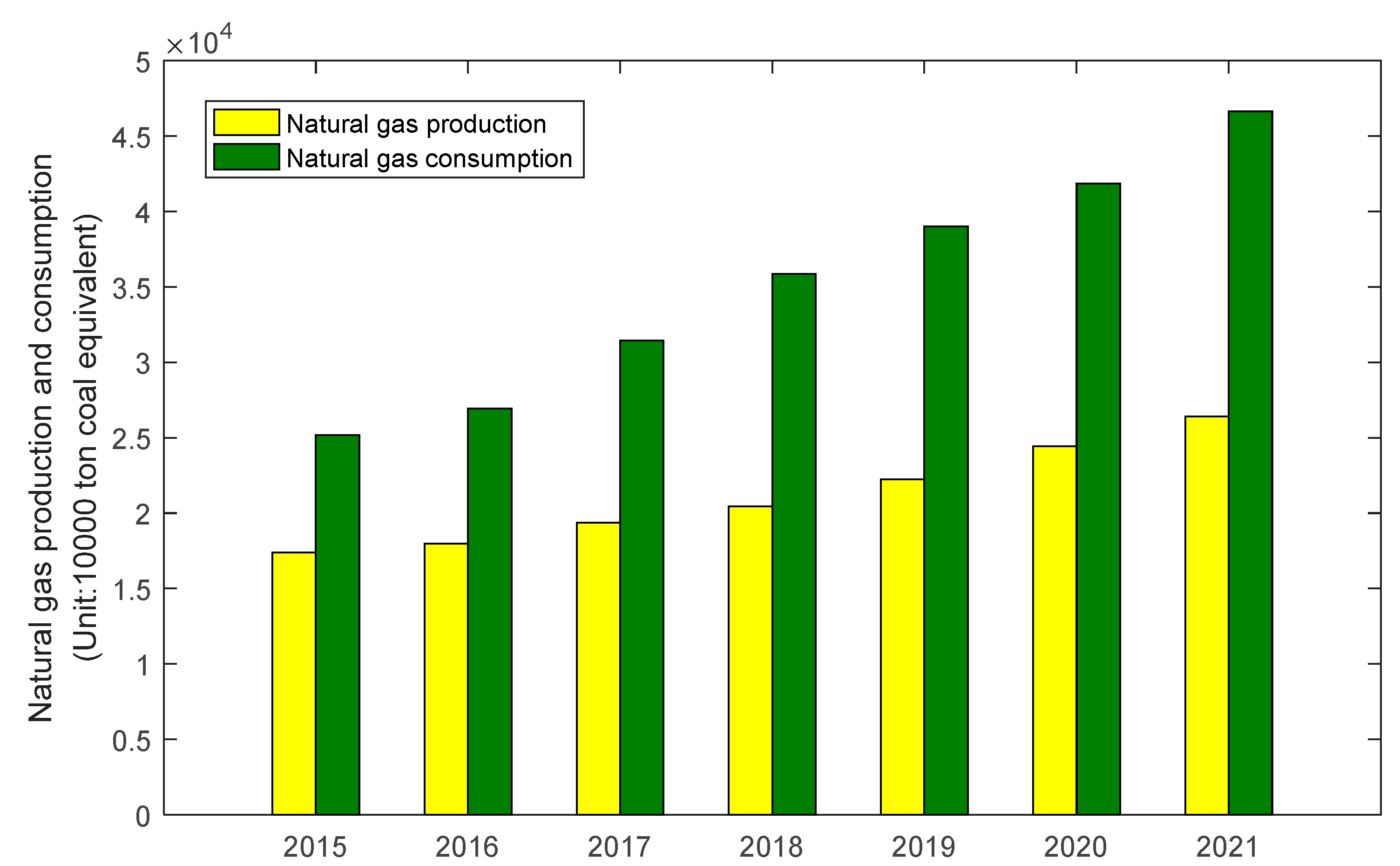
Figure 1. Natural gas production and consumption in China from 2015 to 2021.
Fractalfract 07 00422 g001
Figure 2. Natural gas production in China from 2015 to 2021. (Unit:100 million cubic meters).
Fractalfract 07 00422 g002
Figure 3. Framework diagram of the SFHGM (1,1) model.
Fractalfract 07 00422 g003
Figure 4. The errors and fitting curve of the four models in Case 1.
Fractalfract 07 00422 g004
Figure 5. APES of the four grey models in Case 1.
Fractalfract 07 00422 g005
Figure 6. The errors and fitting curve of the six models in Case 2.
Fractalfract 07 00422 g006
Figure 7. APES of the six grey models in Case 2.
Fractalfract 07 00422 g007
Figure 8. Distribution of natural gas production in each season from 2015 to 2021.
Fractalfract 07 00422 g008
Figure 9. The structural chart of forecasting natural gas production in China.
Fractalfract 07 00422 g009
Figure 10. Fitted and predicted values of Natural gas production in China.
Fractalfract 07 00422 g010
Figure 11. Comparison of the forecast results of the four models (ad).
Fractalfract 07 00422 g011
Figure 12. Error comparison of four models (ad) in the Validation group.
Fractalfract 07 00422 g012
Table 1. The criterion of the MAPE.
MAPE (%)Forecasting AbilityMAPE (%)Forecasting Ability
<10Excellent20–50Reasonable
10–20Good>50Inaccurate
Table 2. Fitting results of different models in Case 1 (Unit: 100 million cubic meters; APE: %).
TimeActual ValueSARIMADGGM (1,1) [19]SGM (1,1) [35]SFHGM (1,1)
Forecasted
Value
APEForecasted
Value
APEForecasted
Value
APEForecasted
Value
APE
2011Q1113.54121.106.66105.197.35113.540.00113.540.00
2011Q2159.65202.4826.83189.4918.69154.793.04153.783.68
2011Q3192.29249.5729.79264.7537.68216.2812.48213.9711.27
2011Q4143.68186.3129.67167.6516.68158.9710.64150.504.75
2012Q1110.03136.9324.45116.285.68111.451.29113.242.92
2012Q2185.66228.9523.32212.9614.70174.346.10177.704.29
2012Q3270.35282.194.38305.4512.98243.559.91244.989.38
2012Q4181.09210.6616.33188.263.96179.011.15171.445.33
2013Q1129.79154.8319.29128.550.96125.503.31128.570.94
2013Q2197.35258.8831.18239.3321.27196.280.54201.292.00
2013Q3247.88319.0828.72352.4042.17274.2510.64277.0211.76
2013Q4182.68238.1930.39211.4015.72201.5910.35193.605.98
2014Q1144.37175.0721.26142.111.57141.332.11145.030.46
2014Q2223.43292.7231.01268.9720.38221.031.07226.851.53
2014Q3345.40360.784.45406.5717.71308.8410.58311.979.68
2014Q4230.92269.3316.63237.382.80227.011.69217.895.64
2015Q1171.34197.9515.53157.18.31159.147.12163.144.79
2015Q2249.75330.9832.52302.2921.04248.900.34255.062.13
2015Q3321.90407.9426.73469.0745.72347.778.04350.618.92
2015Q4244.79304.5324.40266.578.90255.644.43244.790.00
Table 3. Performance evaluation of the prediction accuracies of the four models (2011Q1–2015Q4). (Unit:100 million cubic meters; MAPE: %).
ModelMAERMSEMAPE
SARIMA44.1350.7022.2
DGGM (1,1)36.9052.9416.2
SGM (1,1)11.6016.325.2
SFHGM (1,1)10.9315.514.8
Table 4. The fitting results of different models in Case 2. (Unit:100 million cubic meters; APE: %).
TimeActual ValueSARIMABPNNDGSM (1,1)SFGM (1,1)SGM (1,1)SFHGM (1,1)
Forecasted
Value
APEForecasted ValueAPEForecasted
Value
APEForecasted
Value
APEForecasted
Value
APEForecasted
Value
APE
2016Q1474.20422.9810.80520.499.76462.762.41416.6212.14419.3911.56474.200.00
2016Q2573.80510.8210.98605.195.47518.699.60521.859.05520.029.37540.565.79
2016Q3420.20394.236.18527.3125.49455.468.39420.730.13419.220.23443.045.44
2016Q4598.10532.4510.98434.8227.30552.306.83602.270.70602.980.82606.961.48
2017Q1618.40490.2720.72591.894.29558.979.61499.7119.19503.0218.66676.749.43
2017Q2695.00564.0118.85684.761.47619.5410.86625.929.94623.7310.26695.000.00
2017Q3563.00435.6322.62727.5629.23561.170.32504.6310.37502.8310.69552.531.86
2017Q4783.00578.3326.14522.2333.30668.0414.68722.387.74723.237.63744.364.94
2018Q1873.80546.5437.45537.8638.45675.1322.74599.3631.41603.3430.95820.976.05
2018Q2841.60631.4524.97620.7326.24741.3111.92750.7410.80748.1211.11836.670.59
2018Q3654.3504.5022.90731.9011.86688.815.27605.277.49603.117.82661.351.48
2018Q4850.10641.3024.56682.1019.76801.845.68866.441.92867.472.04886.974.34
Table 5. Performance evaluation of the prediction accuracies of the six models (2016Q1–2018Q4). (Unit:100 million cubic meters; MAPE: %).
ModelMAERMSEMAPE
SARIMA141.08170.014.56
BPNN134.38173.446.42
DGSM (1,1)65.0986.276.02
SFGM (1,1)70.97102.206.83
SGM (1,1)71.13101.496.76
SFHGM (1,1)22.8431.533.73
Table 6. Seasonal index.
QuarterQ1Q2Q3Q4
Seasonal index1.1134641.0029410.9692681.073026
Table 7. Corresponding parameter values of SFHGM (1,1) model.
The Correlation CoefficientThe Development Coefficient   a s Grey Action   b s The Initial Value   x 0 ( 1 ) / f d ( 1 )
Value−0.0165274.8715302.12
Table 8. Forecast values and errors (2015Q1–2021Q4) of four models. (Unit: 100 million cubic meters; APE: %).
TimeActual ValueARIMASGM (1,1)PSO-FGSM (1,1)SFHGM (1,1)
Forecasted ValueAPEForecasted ValueAPEForecasted
Value
APEForecasted
Value
APE
Training stage
2015Q1336.4304.39.54336.40.00336.40.00336.40.00
2015Q2293.0311.76.38297.41.50292.00.34294.60.55
2015Q3301.0290.83.39301.00.00293.12.62293.82.39
2015Q4339.7340.70.29345.91.83338.40.38333.81.74
2016Q1374.0347.67.06345.07.75340.78.90354.75.16
2016Q2315.7328.54.05321.31.77320.21.43326.73.48
2016Q3312.4311.10.42325.24.10326.84.61322.53.23
2016Q4364.9373.22.27373.72.41377.93.56364.50.11
2017Q1387.4390.10.70372.63.82378.72.25385.90.39
2017Q2357.4359.00.45347.12.88353.90.98354.50.81
2017Q3348.4352.21.09351.30.83358.62.93349.30.26
2017Q4386.5390.30.98403.64.42411.96.57394.21.99
2018Q1396.7411.63.76402.61.49410.13.38416.85.07
2018Q2376.9392.54.14375.00.50380.81.03382.51.49
2018Q3380.4396.34.18379.60.21383.70.87376.61.00
2018Q4429.4426.00.79436.01.54438.32.07424.71.09
2019Q1439.8437.00.64434.91.11434.31.25448.82.05
2019Q2424.2408.63.68405.14.50401.45.37411.72.95
2019Q3412.3412.40.02409.80.61402.82.30405.11.75
2019Q4456.6438.24.03470.33.00458.20.35456.60.00
Verification stage
2020Q1483.2462.14.37469.92.75452.46.37482.40.17
2020Q2472.7437.67.43437.67.43416.711.85442.36.43
2020Q3430.4445.33.46443.02.93416.83.16435.21.12
2020Q4518.9479.17.67508.91.93472.98.86490.45.49
2021Q1533.1486.28.80507.74.76465.612.66517.92.85
2021Q2511.5470.68.00472.87.57427.916.34474.87.17
2021Q3473.7477.20.74478.61.03426.99.88467.01.41
2021Q4534.3503.45.78549.82.90483.59.51526.21.52
Table 9. Predicted quarters natural gas production for the period 2022Q1–2024Q4. (Unit:100 million cubic meters).
Year202220232024
Quarter
Q1555.7595.8638.6
Q2509.3546.1585.2
Q3500.9537575.4
Q4564.3604.8648.1
Table 10. The accuracy comparison of the four models for natural gas production(2015Q1–2019Q4).
ModelMAERMSEMAPE (%)
ARIMA10.4712.022.89
SGM (1,1)8.3711.390.07
PSO-FGSM (1,1)9.6113.250.12
SFHGM (1,1)6.578.930.04
Table 11. The accuracy comparison of the four models for natural gas production(2020Q1–2021Q4).
ModelMAERMSEMAPE(%)
ARIMA29.1432.255.78
SGM (1,1)19.4423.603.91
PSO-FGSM (1,1)49.3955.759.83
SFHGM (1,1)16.422.193.27
Disclaimer/Publisher’s Note: The statements, opinions and data contained in all publications are solely those of the individual author(s) and contributor(s) and not of MDPI and/or the editor(s). MDPI and/or the editor(s) disclaim responsibility for any injury to people or property resulting from any ideas, methods, instructions or products referred to in the content.