Article

Determination of a Nonlinear Coefficient in a Time-Fractional Diffusion Equation

1
College of Engineering and Technology, American University of the Middle East, Egaila 54200, Kuwait
2
Department of Basic Sciences, Deanship of Preparatory Year and Supporting Studies, Imam Abdulrahman bin Faisal University, Dammam 34212, KSA, Saudi Arabia
3
Department of Mathematics and Computer Science, College of Science and General Studies, Alfaisal University, Riyadh 11533, KSA, Saudi Arabia
4
Department of Mathematics and Natural Sciences, Faculty of Arts and Sciences, American University of Ras Al Khaimah, Ras al Khaimah 63920, United Arab Emirates
*
Author to whom correspondence should be addressed.
Fractal Fract. 2023, 7(5), 371; https://doi.org/10.3390/fractalfract7050371
Submission received: 24 February 2023 / Revised: 23 April 2023 / Accepted: 24 April 2023 / Published: 29 April 2023

Abstract

:
In this paper, we study direct and inverse problems for a nonlinear time fractional diffusion equation. We prove that the direct problem has a unique weak solution and the solution depends continuously on the coefficient. Then we show that the inverse problem has a quasi-solution. The direct problem is solved by the method of lines using an operator approach. A quasi-Newton optimization method is used for the numerical solution to the inverse problem. The Tikhonov regularization is used to overcome the ill-posedness of the inverse problem. Numerical examples with noise-free and noisy data illustrate the applicability and accuracy of the proposed method to some extent.

1. Introduction

In recent years, different approaches have been provided for the modeling of diffusion in fractal geometry [1,2,3,4,5,6,7,8,9,10]. Those approaches are mainly based on fractional differential equations. In this article we also adopted a similar approach. For the sake of completeness, we give a brief background. One-dimensional mass transport due to diffusion is formulated by
u t = x J u ,
where J u is the diffusive mass flux. For Fickian diffusion, J u is defined by the following equation:
J u = D ( m ) u x ,
where D ( m ) is the diffusion coefficient. Defining the new non-dimensional variables X = x x 0 , τ = t t 0 , U = u u 0 , where x 0 , t 0 and u 0 are the characteristic scales, the Equations (1) and (2) can be given in the non-dimensional form as follows:
1 t 0 U τ = 1 x 0 2 X D ( m ) U X .
If x 0 = t 0 , then the Equations (1) and (2) preserve their original form. However, many experiments with fractal objects show that this correlation does not hold. In this case, it is proved that the-mean square displacement of a random walker < x 2 > t 2 2 + θ , where θ is the index of the anomalous diffusion. Thus, in our case we have the correlation < x 0 2 > t 0 2 2 + θ and it is clear that there are many expressions for the mass flux that correspond to that correlation. For example, the diffusion coefficient may be defined as D ( m ) ( x ) = D f x θ , where the constant D f is the effective diffusion coefficient. Therefore, we obtain the following diffusion equation:
u t = x D f x θ u x .
As another example, the mass flux may be taken proportional to the fractional derivative of concentration with respect to spatial coordinate of the order θ + 1 . In this case, the obtained mass flux is doubtful since the order of the corresponding diffusion equation is greater than 2. For this reason, the following expression for the mass flux is considered:
J u = D f t 1 β x γ u , β > 0 , γ < 1 ,
where β and γ are the order of the temporal and spatial fractional derivatives, respectively. In the expression (5), t β and x γ are spatial and temporal Caputo fractional derivatives and are defined as the following:
x γ u ( x , t ) = γ u ( x , t ) x γ = 1 Γ ( 1 γ ) 0 x ( x ξ ) γ u ( ξ , t ) ξ d ξ ,
t β u ( x , t ) = β u ( x , t ) t β = 1 Γ ( 1 β ) 0 t ( t ξ ) β u ( x , ξ ) ξ d ξ ,
where Γ ( · ) is the Gamma function. We also note that there is another frequently used fractional derivative, so called the Riemann-Liouville fractional derivative, which is defined by
R t β u ( x , t ) = 1 Γ ( 1 β ) t 0 t ( t ξ ) β u ( x , ξ ) d ξ .
These two fractional derivatives agree when the initial condition is zero. Kilbas et al. [11] and Podlubny [12] can be referred for further properties of the Caputo and Riemann-Liouville fractional derivatives. Since the initial condition is zero in our problem, any result found in the literature for one of these holds for the other one. Substituting the temporal and spatial fractional Caputo derivatives in the expression (5), we obtain:
u t = x D f t 1 β γ u x γ ,
where γ and β are coupled in such a way that < x 0 2 > t 0 2 2 + θ is satisfied. It can also be shown that the correlation t 0 = x 0 1 + γ β holds. We can then conclude that θ + 2 = 1 + γ β . By applying the fractional integral operator to both sides of (6), we obtain the following useful form:
β u t β = x D f γ u x γ .
The Equation (7) can be found in the literature on the diffusion phenomena in the chaotic migration of the particles and anomalous contaminant diffusion from a fracture into a porous rock matrix with an alteration zone bordering the fracture, see [13,14,15,16,17] and some of the references cited therein for further reading. In addition, in [7,18], the case where γ = 1 is considered under the assumption the porous medium has a comb-like structure of fractal geometry. We refer the readers to [15] for more details about the Equation (7).
When a porous medium equation is considered, the pressure is taken to be a monotone function of the concentration u. In this case, by using the corresponding Darcy’s Law and the continuity equation, the following nonlinear equation is obtained:
u t + · d ( u ) u = 0 .
The Equation (8) is also known as the Richards’ equation in hydrology [19].
For the convenience of the reader, we present the main steps of the derivation of the governing equation by following [20]. If the fluid particles are trapped in some region for several periods of time s 1 , , s n , the continuity equation becomes
u t = i = 1 n w i · q ( x , t s i ) ,
where w i are some weights. If we consider the case with w i = w ( s i ) Δ s i and Δ s i = s i s i 1 for some weight density w = w ( s ) , and calculate the limit of u t as n, the Equality (9) becomes
u t = 0 t w ( t s ) · q ( x , s ) d s .
The Equation (10) accounts for the fluid particles that can be trapped for any period of time. The function w ( s ) represents the amount of flux of the particles that waits for the time s. Using the choice for w used in [20], we conclude the following:
u t = 1 Γ ( β ) t 0 t ( t s ) β 1 · q ( x , s ) d s = R t 1 β · q .
If we apply the Riemann-Liouville fractional operator I t 1 β to both sides of (11) and take into account the composition formula for the functions with vanishing initial conditions, we obtain
β t β u = · d ( u ) u .
The Equation (12) is also called the generalized Richards equation [21] and can be found in many papers. In [21], the Equation (12) is solved numerically and the solution to the data on horizontal water transport is fitted. The numerical solution is also studied by some authors, see [22,23,24,25]. In [26], magnetic resonance imaging was employed to study water ingress in fine zeolite powders compacted by high pressure. The measured moisture profiles indicate sub-diffusive behavior with a spatio-temporal scaling variable η = x t γ / 2 . In [26], the Equation (12) is used to analyze the data, and an expression that yields the moisture dependence of the generalized diffusivity is derived and applied to their measured profiles. In [27], the authors use a time-fractional diffusion equation for the modeling of the probability density function of displacements. In [28], a method of approximating equations with the Erdelyi-Kober fractional operator which arise in mathematical descriptions of anomalous diffusion has been introduced. A theorem is proven on the exact form of the approximating series. The authors also provide an illustration obtained by the fractional porous-medium equation that is used to model moisture diffusion in building materials.
The authors in [29] look for self-similar solutions for the Equation (12). The resulting similarity equations are of nonlinear integro-differential type. They approximate these equations by an expansion of the integral operator and look for solutions in a power function form. Several applications of the Equation (12) are presented in [30]. In addition to what is already mentioned above, there has been a growing interest in inverse problems with fractional derivatives. These problems are physically and practically very important. Interested readers can be referred to [31,32,33,34,35,36,37,38,39,40,41,42,43] for a deeper understanding of the topic.
In [30], the authors proposed a generalization of Richards’ equation to estimate super-diffusion and sub-diffusion by means of the power-law ruler. Resulting solutions to the fractional Richards’ equation display anomalous non-Boltzmann scaling as a result of fractal medium of heterogeneous media. In [28], a fractional porous-medium equation to model moisture diffusion in building materials is considered. To achieve this goal, the author improved a method of approximating equations by means of Erdélyi-Kober fractional operator which is observed in equations describing anomalous diffusion. In [26], a time-fractional diffusion equation model of anomalous diffusion is adopted to analyze the data of moisture profiles. The authors consider a nonlinear diffusion equation with a time-fractional derivative which is a generalization of the porous medium equation and they find self-similar solutions to that problem in [29].
In this paper, we study an inverse coefficient problem for the nonlinear time-fractional diffusion Equation (12). The difference of our study from the studies in the references [31,32,33,34,35,36,37,38,39,40,41,42,43] is that the unknown of the inverse problem is non-linear, i.e., it depends on the solution u. This is a relatively new topic and there are only a few works, see [44,45,46]. In [44], the unknown coefficient depends on the gradient of the solution and belongs to a set of admissible coefficients. The authors prove that the direct problem has a unique solution and set up the continuous dependence of the solution of the corresponding direct problem on the unknown coefficient. Then, the existence of a quasi-solution of the inverse problem is shown in the appropriate class of admissible coefficients.
In [44], the numerical solutions of the direct and the inverse problems have been introduced and in [45] an application of the governing equation in the materials sciences has been mentioned. An inverse problem for the nonlinear time-fractional diffusion (12) is studied in [46]. In this paper, the authors prove that the direct problem has a unique solution. The existence of a quasi-solution is also proved. However, neither the uniqueness of the solution is proved nor the direct and the inverse problems are solved numerically. Therefore, our study can be considered as the continuation of the series of work in [46] and the works mentioned above on fractional inverse problems.
It is also worth mentioning that some inverse problems are studied for the case β = 1 in (12). For example, in [47], the determination of the unknown coefficient d ( u ) from over-specified data measured at the boundary has been studied. The inverse problem is reformulated as an auxiliary inverse problem and it is shown that this auxiliary problem has at least one solution in a specified admissible class. Finally, the auxiliary problem is approximated by an associated identification problem and some numerical results are presented. In [48], an operator approach is improved by an input-output mapping and it is shown that the mapping is isotonic. This result is used to derive a uniqueness result for the inverse problem.
This paper is organized as follows: In Section 2 we formulate the direct and the inverse problems. Existence and uniqueness for the direct and the inverse problems are discussed in Section 3. The numerical solutions of the direct and the inverse problems are studied in Section 4 and Section 5, respectively. The conclusion and the potential directions of improvement on the problem are presented in Section 6.

2. Formulation of the Direct and the Inverse Problems

In this section we formulate the direct and the inverse problems. First, we consider the following problem:
β u t β = · d ( u ) u + f ( x , y , t ) , ( x , y , t ) Γ T , u ( x , y , t ) = 0 , ( x , y , t ) Γ 3 T Γ 4 T , d ( u ) u y ( x , y , t ) = g 1 ( x , t ) , ( x , y , t ) Γ 1 T , d ( u ) u x ( x , y , t ) = g 2 ( y , t ) , ( x , y , t ) Γ 2 T , u ( x , y , 0 ) = 0 , ( x , y ) Ω ¯ ,
where β is the order of the Caputo fractional time derivative , Ω : = ( 0 , 1 ) × ( 0 , 1 ) , Γ T : = Ω × ( 0 , T ) , Γ i T : = Γ i × ( 0 , T ) , for i = 1 , 2 , 3 , 4 and T > 0 is the end time. We assume that Ω is a bounded simply connected domain with a piece-wise smooth boundary Ω = Γ 1 Γ 2 Γ 3 Γ 4 with Γ i Γ j = , i j . We define Γ i , i = 1 , 2 , 3 , 4 as follows:
Γ 1 : = ( 0 , 1 ) × { 1 } , Γ 2 : = { 1 } × ( 0 , 1 ) , Γ 3 : = ( 0 , 1 ) × { 0 } , Γ 4 : = { 0 } × ( 0 , 1 ) .
The direct problem consists of determining the function u ( x , y , t ) from the problem (13) for the given inputs β , d ( u ) , f ( x , y , t ) , g 1 ( x , t ) and g 2 ( y , t ) . We solve the direct problem (13) in Section 4 by converting the equation in (13) into a fractional system using the method of lines. Next, we define the class of admissible coefficients and the weak solution of the problem (13). We note that, throughout the paper, · and , denote the usual L 2 ( Ω ) norm and inner product, respectively, · X denotes the norm in a Hilbert space X. C ( I ) denotes the set of continuous functions defined on I.
Definition 1.
Let I : = [ 0 , ) . A set D satisfying the following conditions is called the class of admissible coefficients for the problem (13):
d C ( I ) , c 0 d ( s ) c 1 , s I ,
d ( u 1 ) u 1 d ( u 2 ) u 2 · ( u 1 u 2 ) c 2 | | ( u 1 u 2 ) | | 2 , u 1 , u 2 H 0 1 ( Ω ) ,
where c 0 , c 1 , c 2 are positive constants.
Definition 2.
A weak solution for the problem (13) is a function u S β ( Γ T ) : = L 2 0 , T ; H 0 1 ( Ω ) W 2 β 0 , T ; L 2 ( Ω ) such that the integral identity
Ω β u t β v d x d y + Ω d u u · v d x d y = Ω f v d x d y + Γ 3 g 1 v d x + Γ 4 g 2 v d y ,
holds for almost every t [ 0 , T ] and for each v S β ( Γ T ) , where
W 2 β ( 0 , T ) : = u L 2 [ 0 , T ] : β u t β L 2 [ 0 , T ] and u ( 0 ) = 0
is the fractional Sobolev space of order β. We note that S β ( Γ T ) is a Banach space with the norm:
u S β ( Γ T ) = u W 2 β 0 , T ; L 2 ( Ω ) 2 + u L 2 0 , T ; H 0 1 ( Ω ) 2 1 2 .
We consider u ( x , y , t ) as a mapping from t ( 0 , T ) to L 2 ( Ω ) and write as u ( t ) = u ( · , · , t ) .
A weak solution of the problem (13) can also be defined as a solution of the following abstract operator equation
L u + A u = F ,
where L u : = L ^ u , v , L ^ u : = β u t β , L ^ : D ( L ^ ) V V * with the domain D ( L ^ ) = u V : β u t β V * , V : = L 2 0 , T ; H 0 1 ( Ω ) , the nonlinear operator A : V V * is defined by
A u , v : = Ω β u t β v d x d y + Ω d u u · v d x d y ,
and F on V is defined by
F , v : = Ω f v d x d y + Γ 3 g 1 v d x + Γ 4 g 2 v d y .
The inverse problem here consists of determining the pair of functions u ( x , y , t ) , d ( u ) from the problem (13) by means of the additional data u ( x , y , t ) = g ^ 1 ( x , t ) , ( x , y , t ) Γ 1 T and u ( x , y , t ) = g ^ 2 ( y , t ) , ( x , y , t ) Γ 2 T . We solve the inverse problem by minimizing the cost functional defined by (22). For the consistency of the additional data with the data of (13) on Γ 1 T , it is assumed that d ( g ^ 1 ( x , t ) ) ( g 1 ^ ) y ( x , y , t ) = g 1 ( x , t ) on Γ 1 T and d ( g ^ 2 ( x , t ) ) ( g 2 ^ ) y ( x , y , t ) = g 1 ( x , t ) on Γ 2 T .
We denote the solution of the direct problem (13) for a given function d D by u ( x , y , t ; d ) . If the function u ( x , y , t ; d ) also satisfies the additional data above, it is called a strict solution of the inverse problem. Now, we reformulate the inverse problem. For this purpose, we define the input-output map Φ : L 2 ( Γ T ) L 2 ( Γ 3 T ) × L 2 ( Γ 4 T ) as
Φ ( d ) : = u ( x , y , t ; d ) | Γ 3 T × Γ 4 T : = u ( x , y , t ; d ) | Γ 3 T , u ( x , y , t ; d ) | Γ 4 T .
Then, the inverse problem is defined as a solution of the following operator equation:
Φ ( d ) = g , g = ( g ^ 1 ( x , t ) , g ^ 2 ( y , t ) ) L 2 ( Γ 3 T ) × L 2 ( Γ 4 T ) .
However, due to the measurement errors in practice, the exact equality in (21) is usually not achieved. Hence, one needs to introduce the auxiliary (error) functional:
I ( d ) : = 0 T Γ 3 | u ( x , y , t ; d ) g ^ 1 ( x , t ) | 2 d x d t + 0 T Γ 4 | u ( x , y , t ; d ) g ^ 2 ( y , t ) | 2 d y d t ,
and consider the following minimization problem:
I ( d ^ ) = min d D I ( d ) .
A solution of the minimization problem (23) is called a quasi-solution (or approximate solution) of the inverse problem. Evidently, if I ( d ^ ) = 0 , then the quasi-solution d ^ is also a strict solution of the inverse problem.

3. Analysis of the Direct and the Inverse Problems

In this section, we analyse both the direct and the inverse problems. The theoretical aspect of the direct problem (13) is studied in [46]. In this study, the authors prove that the direct problem (13) is well-posed in the sense of Hadamard. For the sake of the reader, we provide some relevant results from [46]. The following theorems state that the direct problem (13) has a unique weak solution that depends continuously on the coefficient d ( u ) . We refer the readers to [46] for detailed proofs.
Theorem 1.
Let d D . Then, the direct problem (13) has a unique weak solution u S β ( Γ T ) . Moreover, for almost every t [ 0 , T ] there exist some constants c , C > 0 such that
β u 2 t β + c u H 0 1 ( Ω ) 2 C f 2 + g 1 L 2 ( Γ 1 ) 2 + g 2 L 2 ( Γ 2 ) 2 .
Theorem 2.
Suppose that a sequence of coefficients { d m } D converges pointwise in [ 0 , ) to a function d D . Then, the sequence of solutions u m : = u ( x , y , t ; d m ) converges to the solution u : = u ( x , y , t ; d ) S β ( Γ T ) , where u : = u ( x , y , t ; d ) denotes the solution of the direct problem (13) for a given coefficient d D .
Next, we prove a theorem for the existence of the solution to the inverse problem. There are two methods in the literature to prove the existence of the solution of inverse problems. The first method is called the monotonicity method, which is based on the continuity and the monotonicity of the input-output mapping. The second method is called quasi-solution method, which is based on minimizing an error functional between the output data and the additional data. We adopt the quasi-solution approach to the inverse problem under consideration. For this purpose, we show that the cost functional defined by (22) is continuous and we construct a compact subset of the class of the admissible coefficients.
Theorem 3.
Assume that a sequence of coefficients { d m } D converges pointwise in [ 0 , ) to a function d D . Then, | I ( d m ) I ( d ) | 0 as n .
Proof. 
Let { d m } D be a sequence of coefficients that converges pointwise in [ 0 , ) to a function d D , u m : = u ( x , y , t ; d m ) and u : = u ( x , y , t ; d ) . Then, we have:
| I ( d m ) I ( d ) | = | 0 T Γ 3 | u m g ^ 1 ( x , t ) | 2 d x d t 0 T Γ 3 | u g ^ 1 ( x , t ) | 2 d x d t + 0 T Γ 4 | u m g ^ 2 ( y , t ) | 2 d y d t 0 T Γ 4 | u g ^ 2 ( y , t ) | 2 d y d t | .
For the first two terms in (24), we have:
0 T Γ 3 | u m g ^ 1 ( x , t ) | 2 d x d t 0 T Γ 3 | u g ^ 1 ( x , t ) | 2 d x d t = | u m g ^ 1 ( x , t ) L 2 ( Γ 3 T ) 2 u g ^ 1 ( x , t ) L 2 ( Γ 3 T ) 2 | u m u L 2 ( Γ 3 T ) × ( u m g ^ 1 ( x , t ) L 2 ( Γ 3 T ) + u g ^ 1 ( x , t ) L 2 ( Γ 3 T ) ) u m u L 2 ( Γ T ) × ( u g ^ 1 ( x , t ) L 2 ( Γ 3 T ) + u g ^ 1 ( x , t ) L 2 ( Γ 3 T ) ) .
By using the fact that u L 2 0 , T ; H 0 1 ( Ω ) K u S β ( Γ T ) for some K > 0 (see [49] for details), we conclude that the following holds for the first term on the right hand side of (25):
u m u L 2 ( Γ T ) u m u L 2 0 , T ; H 0 1 ( Ω ) K u m u S β ( Γ T ) .
From (26) and Theorem 2, we conclude that the first two terms in (24) goes to zero as n . Similarly, we can prove that the last two terms in (24) tend to zero as n . This completes the proof. □
The conditions (14) and (15) arise in the solvability of the direct problem (13) and can be found in some papers, for example see the condition H3 in [50]. In virtue of Theorem 3, it is natural to construct a compact set of admissible coefficients in C ( I ) . For this reason, in addition to the assumptions (14) and (15), we assume that there is a subset D c of D which is equicontinuous, i.e., D c D and for every ϵ > 0 there exists a δ > 0 such that if d D c , s 1 , s 2 I and | s 1 s 2 | < δ , then | d ( s 1 ) d ( s 2 ) | < ϵ . By following Theorem 3 in [51] it can be proved that D c is compact. Then, we obtain the following existence theorem.
Theorem 4.
The inverse problem has at least one quasi-solution in the set of admissible coefficients D c .
Proof. 
The Weierstrass theorem and Theorem 3 guarantees the existence of the solution to the inverse problem is proved. □
The following theorem shows that the input-output operator defined by (20) is a compact operator.
Theorem 5.
Let the conditions (14) and (15) hold. Then, the input-output operator defined by (20) is a compact operator [46].
Since nonlinear equations with compact operators are ill-posed [52], the inverse problem under consideration is also ill-posed.
The following example shows that there exists a sequence { d n } such that u ( x , y , t ; d n ) , ( x , y , t ) Γ 1 T and u ( x , y , t ; d n ) , ( x , y , t ) Γ 2 T converges to zero as n , but d n as n .
Example 1.
For d n ( u ) = n 2 , β = 1 / 2 and f n ( x , t ) = 8 x 3 y 2 t 3 / 2 3 π n 5 2 x t 2 n 3 ( 3 y 2 + x 2 ) , the inverse problem (13) becomes
β u t β = ( n 2 u x ) x + ( n 2 u y ) y + 8 x 3 y 2 t 3 / 2 3 π n 5 2 x t 2 n 3 ( 3 y 2 + x 2 ) , ( x , y , t ) Γ T , u ( x , y , t ) = 0 , ( x , y , t ) Γ 3 T Γ 4 T , n 2 u y ( x , y , t ) = 2 n 3 x 3 t 2 , ( x , y , t ) Γ 1 T , n 2 u x ( x , y , t ) = 3 n 3 y 2 t 2 , ( x , y , t ) Γ 2 T , u ( x , y , 0 ) = 0 , ( x , y ) Ω ¯ .
It can easily be verified that the function u n ( x , y , t ; d n ) = x 3 y 2 n 5 t 2 is the solution of the corresponding direct problem. Obviously, u n ( x , 1 , t ; d n ) and u n ( 1 , y , t ; d n ) converge to zero as n , but d n ( u ) as n .

4. Numerical Solution of the Direct Problem

In this section we introduce the methodology used for solving the direct problem numerically. The main idea is to convert the fractional partial differential equation into a system of fractional ordinary differential equations using the method of lines and vectorization and then solve the resulting system of fractional ordinary differential equations. In addition to the classical method of lines, we adopt the operator approach to approximate derivatives, which reduces computations and memory demand of the algorithm. We first illustrate the methodology over a one-dimensional heat equation. For this purpose, we consider the following one-dimensional problem:
u t = k 2 u x 2 , x ( 0 , 1 ) , t ( 0 , 1 ) , u ( x , 0 ) = h ( x ) , x ( 0 , 1 ) , u ( 0 , t ) = f ( t ) , u ( 1 , t ) = g ( t ) , t ( 0 , 1 ) .
For a given positive integer M, let x i = i Δ x for i = 0 , 1 , 2 , , M with Δ x = 1 / M . Additionally, let u i ( t ) denote the approximation of the solution at the node ( x i , t ) for i = 0 , 1 , 2 , , M , where u 0 ( t ) = f ( t ) and u M ( t ) = g ( t ) . We approximate the given equation by the following system of ordinary differential equations for u i ’s:
d u i d t = k u i + 1 2 u i + u i 1 Δ x 2 , t ( 0 , 1 ) , i = 1 , , M 1 , u i ( 0 ) = h ( x i ) , i = 1 , , M 1 .
Given the vector of approximate solutions at each node without boundaries, [ u i ] = [ u 1 , u 2 , , u M 1 ] , we define the left and right shift operators as
L S ( [ u i ] ) = [ u i + 1 ] and R S ( [ u i ] ) = [ u i 1 ] , i = 0 , 1 , 2 , , M 1 .
Then, the system of ordinary differential equations given in (28) can be written as follows:
d u i d t = L S ( [ u i ] ) 2 [ u i ] + R S ( [ u i ] ) Δ x 2 ,
with d u i d t = d u 1 d t , d u 2 d t , , d u M 1 d t being the vector of time derivatives at the discretized nodes. To illustrate how we generalize the shift-operator approach to higher dimensional partial differential equations, we consider the following two-dimensional problem:
u t = 2 u x 2 + 2 u y 2 + f ( x , y , t ) , ( x , y , t ) Γ T , u ( x , y , 0 ) = h ( x , y ) , ( x , y ) Ω , u ( x , y , t ) = g ( x , y , t ) , ( x , y ) Ω , t ( 0 , 1 ) .
Let x i = i Δ x , i = 0 , , M and y j = j Δ y , j = 0 , 1 , 2 , , N with Δ x = 1 / M and Δ y = 1 / N . Additionally, let u i j ( t ) denote the solution at point ( x i , y j ) at a time t ( 0 , 1 ) , where u 0 j = g ( 0 , y j , t ) , u M j = g ( 1 , y j , t ) , u i 0 = g ( x i , 0 , t ) and u i N = g ( x i , 1 , t ) . Then, the centered difference approximation of the time derivative at point ( x i , y j ) will be
d u i j d t = u i + 1 j 2 u i j + u i 1 j Δ x 2 + u i j + 1 2 u i j + u i j 1 Δ y 2 + f ( x i , y j , t ) ,
with i = 1 , , M 1 and j = 1 , , N 1 . This approximation can be vectorized by defining the solution matrix at the interior points [ u i j ] = u ( x i , y j ) with i = 1 , , M 1 and j = 1 , , N 1 . We define the left and right shift operators on the matrix [ u i j ] of solution approximations at the interior points as follows:
L S ( [ u i j ] ) = [ u i + 1 j ] and R S ( [ u i j ] ) = [ u i 1 j ] ,
with i = 1 , , M 1 and j = 1 , , N 1 . Then the matrices of the centered difference approximations to the first order derivatives can be expressed as follows:
[ u x i j ] = L S ( [ u i j ] ) R S ( [ u i j ) ] 2 Δ x ,
[ u y i j ] = L S ( [ u i j ] ) R S ( [ u i j ] ) 2 Δ y ,
where [ a i j ] denotes the transpose of the matrix [ a i j ] . The matrices of the centered difference approximations to the second order derivatives, [ u x x i j ] , [ u y y i j ] , and [ u x y i j ] can be obtained by applying L S and R S operators to the matrices of the first order derivative approximations given in (32) and (33). Then, (31) can be expressed in matrix form as follows:
d u i j d t = [ u x x i j ] + [ u y y i j ] + [ f ( x i , y j , t ) ] ,
with initial condition matrix [ u i j ( 0 ) ] = [ h ( x i , y j ) ] of size M 1 × N 1 .
Next, we consider the following time-fractional problem:
β u t β = f ( x , y , t , u , u x , u y , u x x , u y y , u x y ) , ( x , y , t ) Γ T , u ( x , y , 0 ) = h ( x , y ) ( x , y ) Ω , u ( x , y , t ) = g ( x , y , t ) , ( x , y ) Ω , t ( 0 , 1 ) .
The vectorized method of lines approach described in examples above results in the following difference approximation for the equation in (35):
β u i j t β = f ( [ x i j ] , [ y i j ] , t , [ u i j ] , [ u x i j ] , [ u y i j ] , [ u x x i j ] , [ u y y i j ] , [ u x y i j ] ) ] ,
with [ u i j ( 0 ) ] = [ h ( x i , y j ) ] [ x i j ] = [ x i ] 1 × M 1 [ 1 ] N 1 × 1 and [ y i j ] = [ y j ] N 1 × 1 [ 1 ] M 1 × 1 , where ⊗ denotes the Kronecker matrix product. We solve this system of nonlinear fractional ordinary differential equations using a Matlab implementation of the Adam-Bashfort-Moulton(ABM) type predictor-corrector method given in [53]. Detailed convergence and stability analysis are considered both in [54,55]. In [54], it is concluded that if the solution under consideration is sufficiently smooth, the method has uniform convergence of order h 2 for β > 1 , and of order h 1 + β for β < 1 , respectively. It is further shown by numerical examples that, these bounds are strict and cannot be improved.
The ABM is a Predict-Evaluate-Correct-Evaluate (PECE)-type method. That is, for the approximation at the time nodes t k , and corresponding approximations, y j y ( t k ) at each k t h step, there are two approximations computed for the next node, namely, predictor, y p ( t k + 1 ) , and using the predictor, the corrector approximation y c ( t k + 1 ) is obtained and used in the calculation. The approximation error is obtained by finding the difference of predictor and corrector approximations. There are two main advantages of using a PECE-type method compared to the classical equivalent-order explicit methods. The first benefit of using an algorithm of type PECE is the high accuracy and stability, see [55,56,57,58]. For fractional ordinary differential equations, it has been shown that the stability and accuracy remains high compared to equivalent-order numerical methods, see [53,54,55]. The second advantage of using a PECE-type numerical algorithm is that these methods use variable time steps that reduce the computational cost of the approximation. The method can control the time steps by using the difference between the corrector and the predictor approximations. When the difference is smaller than the desired level of accuracy with the current time step, this can be used as an indication that the solver is in a non-stiff area, and consequently time steps are increased in an adaptive manner.
The idea of combining the method of lines approach to reduce the given fractional partial differential equation to a system of fractional ordinary differential equations and using shift operators in the evaluation of the right-hand side of the PDE can prove to be useful in terms of memory and computation compared to similar operator approaches, such as that of Podlubny’s intuitive matrix operator approach, see [59,60], depending on the problem under consideration. In terms of memory, the method of lines approach uses matrices of size M × N . Whereas in Podlubny’s Matrix Operator approach, the matrices under consideration are of size M × N × K where K is the number of mesh points in t direction used in the calculation. So, the method of lines approach is able to improve the memory demand of the calculations. However, this improvement in memory demand comes at the cost of calculation of the right-hand side function at each time step. Similarly, Podlubny’s matrix operator approach may also face the computational challenges depending on the complexity of the fractional partial differential equation. This is because the method requires solving nonlinear algebraic matrix equation of very high dimensions. Hence, the very nature of the question under consideration is the sole factor in choosing the numerical method to apply.
The first series of the numerical simulations is related to numerical solution of the direct problem. For this purpose, the function u ( x , y , t ) = t x 2 y 2 is taken to be the analytic solution of the equation β u t β = ( d ( u ) u x ) x + ( d ( u ) u y ) y + f ( x , y , t ) , with the function d ( u ) = 1 + u and appropriately chosen source function f ( x , y , t ) . The boundary conditions are found from the trace of the function u ( x , y , t ) = t x 2 y 2 on Ω . First, we check the difference between the numerical solution u num and the exact solution u e x a c t = u ( x , y , t ) = t x 2 y 2 . The absolute error between u num and u exact is defined by u num u exact , where · denotes the supremum norm, which is taken over all x , y , t where x [ 0 , 1 ] , y [ 0 , 1 ] and t [ 0 , 0.3 ] . The software is simulated for different values of the system parameters to evaluate their effect on the absolute error and the simulation time. The time step is taken Δ t = 10 5 . We note that a decay in the time step may lead to and increase in the simulation time and has almost no effect on the computations. However, there is a subtle relation between the number of time nodes and x-y nodes. Increasing Δ t = 10 5 when t [ 0 , 0.3 ] affects the stability of the simulation when higher number of x-y nodes is used. We simulated the solution for M = N = 5 , M = N = 10 and M = N = 20 for β = 0.6 and β = 0.7 . We show the results with computation times in Table 1 and Table 2. We observe that M = N = 5 serves the best time and the least absolute error. In addition, it appears that as β increases towards 1, the absolute error decreases. Hence, the time step and number of discretization nodes for the remaining simulations are chosen to be seemingly the optimal values of 10 5 and M = N = 5 .
Next, we consider the ill-posedness of the inverse problem. A problem is called to be well-posed in the Hadamard sense if the solution exists, unique and depends continuously on the input data. Failure to comply any of the mentioned properties makes the given problem ill-posed. To show that the inverse problem under consideration is ill-posed, we simulate the direct problem for a 1 ( u ) = 1 + u and a 2 ( u ) = 3 + u . The functions u 1 ( x , y , 1 ) and u 2 ( x , y , 1 ) are found through the numerical solution. 
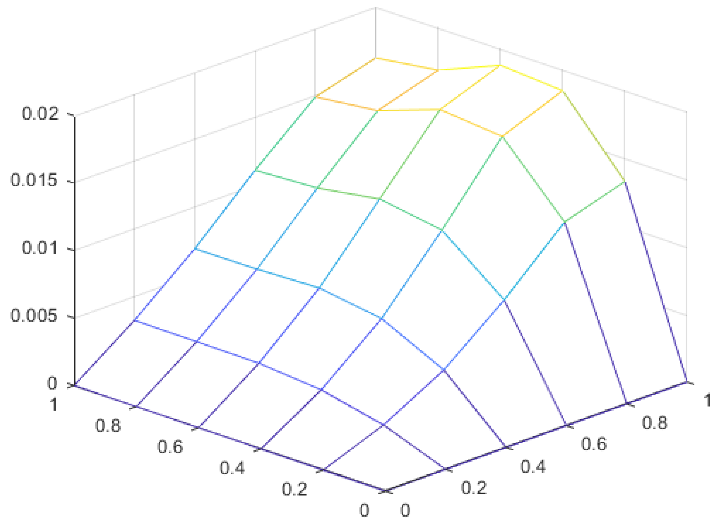
Figure 1 shows that the graph of the difference µ u 1 ( x , y , 1 ) u 2 ( x , y , 1 ) where we see the solutions on both Γ 3 T and Γ 4 T are very close to each other with an absolute difference less than 0.02 .

5. Numerical Solution of the Inverse Problem

We assume that for a fixed β , the following problem has the solution u ˜ ( x , y , t ) for the specific functions d ˜ , f ( x , y , t ) , g 1 ( x , t ) and g 2 ( y , t ) . In the inverse problem, we aim to try to find the function d ˜ when only u ˜ ( x , 1 , t ) and u ˜ ( 1 , y , t ) are known about the solution u ˜ while the boundary conditions and f ( x , y , t ) are known and fixed. The boundaries are the same as in the Equation (13).
β u t β = · d ( u ) u + f ( x , y , t ) , ( x , y , t ) Γ T , u ( x , y , t ) = 0 , ( x , y , t ) Γ 3 T Γ 4 T , d ( u ) u y ( x , y , t ) = g 1 ( x , t ) , ( x , y , t ) Γ 1 T , d ( u ) u x ( x , y , t ) = g 2 ( y , t ) , ( x , y , t ) Γ 2 T , u ( x , y , 0 ) = 0 , ( x , y ) Ω ¯ .
In our experiments, first we fix our solution u ˜ ( x , y , t ) as t x 2 y 2 and the specific function d ( u ) beforehand. By using them we find the exact values of g 1 ( x , t ) , g 2 ( x , t ) , whereas f ( x , y , t ) is found numerically. Now g 1 ( x , t ) , g 2 ( x , t ) and f ( x , y , t ) at hand, we take u ˜ ( 1 , y , t ) = t y 2 and u ˜ ( x , 1 , t ) = t x 2 as additional conditions for the inverse problem and we try to find d ( u ) . To do this, we set up the following error functional for each function d as in (23):
I ( d ) : = 0 T 0 1 | u ( x , y , t ; d ) u ˜ ( x , 1 , t ) | 2 d x d t + 0 T 0 1 | u ( x , y , t ; d ) u ˜ ( 1 , y , t ) | 2 d y d t
where u ( x , y , t ; d ) denotes the solution of the direct problem for the function d. We can easily deduce that I ( d ˜ ) = 0 . Thus, we expect to find d ˜ ( u ) as the minimizer of the error functional.
We carry out the experiment for the noise-free data and the noisy data. For the noisy data, we add the noise 0.1 ϕ 1 ( x , t ) and 0.1 ϕ 2 ( x , t ) to g 1 ( x , t ) and g 2 ( x , t ) , respectively. Here, ϕ 1 ( x , t ) and ϕ 2 ( x , t ) assume the values in the form of 0.1 × m ( x , t ) where m takes random values from [ 1 , 1 ] .
We will use polynomials to approximate the minimum d ˜ in the light of Theorem 2. For n > 0 , we assume that d ( u ) = d n u n + + d 0 . Thus, I ( d ) is a function of the vectors ( d , d 0 ) R n + 1 where d = ( d n , d 1 ) .
We apply the BGFS method, a Quasi-Newton method, to minimize the function. The method requires the evaluation of the gradient of the function I ( d ) . The BGFS method approximates the Hessian of the error function with a cubic line search procedure in each step. For further reading, we refer [24]. We choose the stopping criteria for the algorithm as | | I ( d ) | | < 10 6 . The integration in I ( d ) is approximated by the trapezoid rule.
In the experiments, in accordance with the observations given in Section 4 we assume β = 0.7 for the order of fractional time derivative, M = N = 5 are used to make a mesh-grid for x and y on [ 0 , 1 ] × [ 0 , 1 ] and time step is taken as t = 10 5 with upper bound T = 0.3 .
We consider the variable d ( u ) as a second degree polynomial. Hence, I ( d ) is treated as a function of three variables. The initial points are chosen to be close to the coefficients of the second degree Taylor polynomial of d ˜ ( u ) , a random number between 0 and 1 is added to or subtracted from each component. In the Table 3, Table 4, Table 5, Table 6, Table 7, Table 8, Table 9, Table 10 and Table 11, we provide the value of I ( d ) for the final d, i.e., d final calculated by the algorithm. We also provide the relative error between the solution of the direct problem for the calculated value of d final and u = t x 2 y 2 . The relative error is given by
| | u final ( x , y , t ) t x 2 y 2 | | | | t x 2 y 2 | | ,
where | | · | | is estimated by the maximum value of the function on the meshgrid on [ 0 , 1 ] × [ 0 , 1 ] × [ 0 , 0.3 ] .
The inverse problem is an ill-posed problem and it is sensitive to the noise. To deal with the noisy data, we use Tikhonov regularization in the error functional and define it as:
I ( d ) : = 0 T 0 1 | u ( x , y , t ; d ) u ˜ ( x , 1 , t ) | 2 d x d t + 0 T 0 1 | u ( x , y , t ; d ) u ˜ ( 1 , y , t ) | 2 d y d t + λ | | d | | 2 ,
where | | · | | is the Euclidean norm. We run the algorithm for different regularization parameter λ with the same initial values and present the best results according to the relative error.
Experiment 1.
The correct d ( · ) is d ˜ ( u ) = 2 sin ( u ) + cos ( u ) , whose second degree Taylor polynomial is 0.5 u 2 + 2 u + 1 . Table 3 and Table 4 show the results for the noise-free and noisy data, respectively. Table 5 shows the best results for different values of the regularization parameter λ .
Experiment 2.
The correct d ( · ) is d ˜ ( u ) = u 2 + u + 1 . Table 6 and Table 7 show the results for the noise-free and noisy data, respectively. Table 8 shows the best results for different values of the regularization parameter λ .
Experiment 3.
The correct d ( · ) is d ˜ ( u ) = e u whose second degree Taylor polynomial is 0.5 u 2 + u + 1 . Table 9 and Table 10 show the results for the noise-free and noisy data, respectively. Table 11 shows the best results for different values of the regularization parameter λ .
Since the algorithm is based on approaching d ( u ) with polynomials and the error function is a function of three variables, the second degree Taylor polynomials of the correct d ( u ) ’s are expected to be attained by the algorithm for each initial point.
In all experiments with noise-free data, we notice that the algorithm finds the linear coefficients of the target Taylor polynomial for almost all initial points, while it mostly fails to reach the nonlinear coefficient, i.e., the coefficient of u 2 of the target Taylor polynomial for most of the initial points. However, the coefficients of the final d ( u ) ’s with the least relative errors almost match the coefficient of u 2 of the target Taylor polynomial. In all of the experiments, the relative error for the solution u corresponding to each final polynomial d ( u ) is observed to fluctuate between 0.0001 and 0.007. Another observation for noise-free experiments is that the relative error for the corresponding u increases with I ( d ) .
In the experiments that are carried out with noisy data, there is a remarkable behavior in the error function: I ( d final ) stays around 0.002 for almost all initial points. The relative error for all initial points and experiments fluctuate between 0.001 and 0.009. So the relative error increases up to 10 times. One observation about the experiments with noisy data is that even though the linear coefficients of d final are more distanced from the linear coefficients of the expected Taylor polynomials, they still seem to accumulate around the expected linear coefficients. The nonlinear coefficients look far from the expected.
The experiments show that the linear part of the d ( u ) is stable with respect to the noise. This is most probably due to the constraints imposed by the method used in the solution of the direct problem. Note that we have a stable solution for t in [ 0 , 0.3 ] with = 10 5 .
For the noisy data, we apply the Tikhonov regularization. The regularization parameters are very close to zero, i.e., the values that are less than 10 7 results in reliable results. In addition, it has been observed that the linearization of d ( u ) is robust against the noise. It appears that the robustness of the linear part increases as β approaches to 1. In the experiments with β = 0.6 , (not shown in this article) the results have shown that the error is higher and that the final points are found to be beyond the expected. So, we can conclude that the problem becomes more ill-posed as β decreases.
We also note that one can also use trust region methods to minimize the error functional. Indeed, some preliminary tests have been carried out with trust region method and the BGFS method. A significant difference in the computation time was observed between two optimization methods. For this reason, the BGFS method was chosen as the primary algorithm for this study.

6. Concluding Remarks

We study an inverse problem for the nonlinear time fractional equation u t β = · ( d ( u ) u ) + f ( x , y , t ) . We solve the direct problem by converting it into a system of fractional ODEs using the method of lines and vectorization. In doing so, we adopted the operator approach to approximate the derivatives that reduces computational and memory demand of the algorithm. After we solve the direct problem, we reformulate the inverse problem as a minimization problem. Then we solve the minimization problem by using the BGFS method and a Quasi-Newton method. The inverse problem is solved for both noise-free and noisy data. When solving the direct problem, we observe that as the order of fractional time derivative approaches to the value 1, the numerical solution approximates the exact solution in much faster and reliable manner. Additionally, it appears that there is a subtle relation between the size of the interval and time steps used in the numerical scheme. We observe that M = N = 5 provides the best performance in terms of the minimum simulation time and the absolute error. The numerical results of the experiments show that solving the inverse problem that we examined in this article using the error functional with the help of polynomials and solving the direct problem with the method of lines work well together. However, the computational constraints resulting from the discussion of the solution of the direct problem makes the problem a bit restrictive on the meshgrid and time interval. The experiments with the noise-free data verifies the theoretical results, i.e., the existence of a unique quasi-solution.The experiments with noisy data show that the linear part of the d ( u ) shows a robust behavior against the noise. Finally, the values of β away from 1 results in unstable results, that is, the problem becomes more ill-posed.
The authors of this paper plan to study a set of three partial differential equations involving time-fractional derivatives and nonlinear diffusion operators. After we prove that the direct problem is a well-posed problem, we define the inverse problem. The inverse problem may be either an inverse parameter problem, or an inverse coefficient problem, or an inverse source problem. Then we study the existence and uniqueness of the solution and solve the inverse problem by the method presented in this paper.

Author Contributions

Conceptualization, S.T. and S.U.; methodology, S.T., S.U., M.Z., R.T. and R.A.-H.; software, M.Z., R.T.; validation, M.Z., R.T., S.T., S.U. and R.A.-H.; formal analysis, S.T. and S.U.; writing—original draft preparation, M.Z., R.T., S.T., S.U. and R.A.-H.; writing—review and editing, M.Z., R.T., S.T., S.U. and R.A.-H.; visualization, M.Z. and R.T.; supervision, S.T., S.U. and R.A.-H.; project administration, S.T. and S.U. All authors have read and agreed to the published version of the manuscript.

Funding

This research received no external funding.

Data Availability Statement

Data is contained within the article.

Conflicts of Interest

The authors declare no conflict of interest.

References

  1. Campos, D.; Fort, J.; Mendez, V. Propagation through fractal media: The Sierpinski gasket and the Koch curve. Europhys. Lett. 2004, 68, 769–775. [Google Scholar] [CrossRef]
  2. Dinariyev, O.Y. The pressure build-up curve for a fractal cracked porous medium. Linear theory. J. Appl. Math. Mech. 1994, 58, 755–758. [Google Scholar] [CrossRef]
  3. Anh, D.H.N.; Hoffmann, K.H.; Seeger, S.; Tarafdar, S. Diffusion in disordered fractals. Europhys. Lett. 2005, 70, 109–115. [Google Scholar] [CrossRef]
  4. Essex, C.; Davison, M.; Schulsky, C.; Franz, A.; Hoffmann, K. The differential equation describing random walks on the Koch curve. J. Physics A Math. Gen. 2001, 34, 8397–8406. [Google Scholar] [CrossRef]
  5. Fomin, S.; Chugunov, V.; Hashida, T. Non-Fickian mass transport in fractured porous media. Adv. Water Resour. 2011, 34, 205–214. [Google Scholar] [CrossRef]
  6. Giona, M.; Roman, H.E. Fractional diffusion equation on fractals: One-dimensional case and asymptotic behavior. J. Phys. A Math. Gen. 1992, 25, 2093–2105. [Google Scholar] [CrossRef]
  7. Nigmatullin, R.R. The realization of the generalized transfer equation in a medium with fractal geometry. Phys. Stat. Sol. 1986, 133, 425–430. [Google Scholar] [CrossRef]
  8. O’Shaughnessy, B.; Procaccia, I. Diffusion on fractals. Phys. Rev. A 1985, 32, 3073–3083. [Google Scholar] [CrossRef] [PubMed]
  9. Sibatov, R.T.; Uchaikin, V.V. Fractional differential approach to dispersive transport in semiconductors. Uspekhi Fizicheskih Nauk 2009, 179, 1079–1104. [Google Scholar] [CrossRef]
  10. Uchaikin, V.V. The Fractional Derivatives Method; Artishok Press: Ul’yanovsk, Russia, 2008. [Google Scholar]
  11. Kilbas, A.A.; Srivastava, H.M.; Trujillo, J.J. Theory and Applications of Fractional Differential Equations; Elsevier: Amsterdam, The Netherlands, 2006. [Google Scholar]
  12. Podlubny, I. Fractional Differential Equations; Academic Press: San Diego, CA, USA, 1999. [Google Scholar]
  13. Del-Castillo-Negrete, D.; Carreras, B.A.; Lynch, E. Front dynamics in reaction-diffusion systems with Lévy flights: A fractional diffusion approach. Phys. Rev. Lett. 2003, 91, 018302. [Google Scholar] [CrossRef]
  14. Fomin, S.; Chugunov, V.; Hashida, T. Application of Fractional Differential Equations for Modeling the Anomalous Diffusion of Contaminant from Fracture into Porous Rock Matrix with Bordering Alteration Zone. Transp. Porous Media 2010, 81, 187–205. [Google Scholar] [CrossRef]
  15. Fomin, S.; Chugunov, V.; Hashida, T. Mathematical Modeling of Anomalous Diffusion in Porous Media. Fract. Differ. Calc. 2011, 1, 1–28. [Google Scholar] [CrossRef]
  16. Li, G.; Zhang, D.; Jia, X.; Yamamoto, M. Simultaneous inversion for the space-dependent diffusion coefficient and the fractional order in the time fractional diffusion equation. Inverse Probl. 2013, 29, 065014. [Google Scholar] [CrossRef]
  17. Metzler, R.; Klafter, J. The random walks guide to anomalous diffusion: A fractional dynamics approach. Phys. Rep. 2000, 339, 1–77. [Google Scholar] [CrossRef]
  18. Nigmatulin, R.R. To the theoretical explanation of the universal response. Phys. Stat. Sol. B 1984, 123, 739–745. [Google Scholar] [CrossRef]
  19. Richards, L.A. Capillary conduction of liquids through porous mediums. J. Appl. Phys. 1931, 1, 318–333. [Google Scholar] [CrossRef]
  20. Plociniczak, L. Analytical studies of a time-fractional porous medium equation. Derivation, approximation and applications. Commun. Nonlinear Sci. Numer. Simulat. 2015, 24, 169–183. [Google Scholar] [CrossRef]
  21. Pachepsky, Y.; Timlin, D.; Rawls, W. Generalized Richards equation to simulate water transport in unsaturated soils. J. Hydrol. 2003, 272, 3–13. [Google Scholar] [CrossRef]
  22. Gerasimov, D.N.; Kondratieva, V.A.; Sinkevich, O.A. An anomalous non-self-similar infiltration and fractional diffusion. Phys. D Nonlinear Phenom. 2010, 239, 1593–1597. [Google Scholar] [CrossRef]
  23. Gerolymatou, E.; Vardoulakis, I.; Hilfer, R. Modeling infiltration by means of a non-linear fractional diffusion model. J. Phys. D Appl. Phys. 2006, 39, 4104–4110. [Google Scholar] [CrossRef]
  24. Nocedal, J.; Wright, S. Numerical Optimization; Springer Science & Business Media: Berlin/Heidelberg, Germany, 2006. [Google Scholar]
  25. Shen, S.; Liu, F.; Liu, Q.; Anh, V. Numerical simulation of anomalous infiltration in porous media. Numer. Algorithm 2015, 68, 443–454. [Google Scholar] [CrossRef]
  26. Azevedo, E.N.d.; Souza, P.L.d.; Souza, R.E.d.; Engelsberg, M. Concentration-dependent diffusivity and anomalous diffusion: A magnetic resonance imaging study of water ingress in porous zeolite. Phys. Rev. E 2006, 73, 011204. [Google Scholar] [CrossRef] [PubMed]
  27. Vargas, W.L.; Palacio, L.E.; Dominguez, D.M. Anomalous transport of particle tracers in multidimensional cellular flows. Phys. Rev. E 2003, 67, 026314. [Google Scholar] [CrossRef]
  28. Plociniczak, L. Approximation of the Erdelyi-Kober operator with applications to the time-fractional porous medium equation. Siam J. Appl. Math. 2014, 74, 1219–1237. [Google Scholar] [CrossRef]
  29. Plociniczak, L.; Okrasinska, H. Approximate self-similar solutions to a nonlinear diffusion equation with time-fractional derivative. Phys. D 2013, 261, 85–91. [Google Scholar] [CrossRef]
  30. Sun, H.; Meerschaert, M.M.; Zhang, Y.; Zhu, J.; Chen, W. A fractal Richards equation to capture the non-Boltzmann scaling of water transport in unsaturated media. Adv. Water Resour. 2013, 52, 292–295. [Google Scholar] [CrossRef] [PubMed]
  31. Cheng, J.; Nakagawa, J.; Yamamoto, M.; Yamazaki, T. Uniqueness in an inverse problem for a one-dimensional fractional diffusion equation. Inverse Probl. 2009, 25, 115–131. [Google Scholar] [CrossRef]
  32. Jin, B.; Rundell, W. An inverse problem for a one-dimensional time-fractional diffusion problem. Inverse Probl. 2012, 28, 075010. [Google Scholar] [CrossRef]
  33. Liu, J.J.; Yamamoto, M. A backward problem for the time-fractional diffusion equation. Appl. Anal. 2010, 89, 1769–1788. [Google Scholar] [CrossRef]
  34. Sakamoto, K.; Yamamoto, M. Inverse source problem with a final overdetermination for a fractional diffusion equation. Math. Control. Rel. Fields. 2011, 4, 509–518. [Google Scholar] [CrossRef]
  35. Sakamoto, K.; Yamamoto, M. Initial value/boundary value problems for fractional diffusion-wave equations and applications to some inverse problems. J. Math. Anal. Appl. 2011, 382, 426–447. [Google Scholar] [CrossRef]
  36. Xu, X.; Cheng, J.; Yamamoto, M. Carleman esimate for a fractional diffusion equation with half order and application. Appl. Anal. 2011, 90, 1355–1371. [Google Scholar] [CrossRef]
  37. Yamamoto, M.; Zhang, Y. Conditional stability in determining a zeroth-order coefficient in a halforder fractional diffusion equation by a Carleman estimate. Inverse Probl. 2012, 28, 105010. [Google Scholar] [CrossRef]
  38. Zhang, Y.; Xu, X. Inverse source problem for a fractional diffusion equation. Inverse Probl. 2011, 27, 035010. [Google Scholar] [CrossRef]
  39. Tatar, S.; Tinaztepe, R.; Ulusoy, S. Determination of an unknown source term in a space-time fractional diffusion equation. J. Fract. Calc. Appl. 2015, 6, 94–101. [Google Scholar]
  40. Tatar, S.; Tinaztepe, R.; Ulusoy, S. Simultaneous inversion for the exponents of the fractional time and space derivatives in the space-time fractional diffusion equation. Appl. Anal. 2016, 95, 1–23. [Google Scholar] [CrossRef]
  41. Tatar, S.; Ulusoy, S. A uniqueness result in an inverse problem for a space-time fractional diffusion equation. Electron. J. Differ. Equ. 2013, 258, 1–9. [Google Scholar]
  42. Tatar, S.; Ulusoy, S. An inverse source problem for a one-dimensional space-time fractional diffusion equation. Appl. Anal. 2015, 94, 2233–2244. [Google Scholar] [CrossRef]
  43. Tuan, N.H.; Long, L.D.; Tatar, S. Tikhonov regularization method for a backward problem for a inhomogeneous time-fractional diffusion equation. Appl. Anal. 2018, 97, 842–863. [Google Scholar]
  44. Tatar, S.; Ulusoy, S. Analysis of Direct and Inverse Problems for a Fractional Elastoplasticity Model. Filomat 2017, 31, 699–708. [Google Scholar] [CrossRef]
  45. Tatar, S.; Tinaztepe, R.; Zeki, M. Numerical Solutions of Direct and Inverse Problems for a Time Fractional Viscoelastoplastic Equation. Asce J. Eng. Mech. 2017, 143, 04017035. [Google Scholar] [CrossRef]
  46. Tatar, S.; Ulusoy, S. An inverse problem for a nonlinear diffusion equation with time-fractional derivative. J. Inverse Ill-Posed Probl. 2017, 25, 185–193. [Google Scholar] [CrossRef]
  47. Canon, J.R.; Duchateau, P. An inverse problem for a nonlinear diffusion equation. Siam J. Appl. Math. 1980, 39, 272–289. [Google Scholar] [CrossRef]
  48. Duchateau, P. Monotonicity and Uniqueness Results in Identifying an Unknown Coefficient in a Nonlinear Diffusion Equation. Siam J. Appl. Math. 1981, 41, 310–323. [Google Scholar] [CrossRef]
  49. Li, X.; Xu, C. Existence and uniqueness of the weak solution of the space-time fractional diffusion equation and a spectral method approximation. Commun. Comput. Phys. 2010, 8, 1016–1051. [Google Scholar]
  50. Manimaran, J.; Shangerganesh, L.; Debbouche, A.; Cortés, J.-C. A time-fractional HIV infection model with nonlinear diffusion. Results Phys. 2021, 25, 104293. [Google Scholar] [CrossRef]
  51. Ou, Y.H.; Hasanov, A.; Liu, H.L. Inverse coefficient problems for nonlinear parabolic differential equations. Acta Math. Sin. Engl. Ser. 2008, 24, 1617–1624. [Google Scholar] [CrossRef]
  52. Engl, H.W.; Kunisch, K.; Neubauer, A. Convergence rates for Tikhonov regularisation of non-linear ill-posed problems. Inverse Probl. 1989, 5, 523–540. [Google Scholar] [CrossRef]
  53. Diethelm, K.; Freed, A.D. The Frac PECE subroutine for the numerical solution of differential equations of fractional order. In Forschung und Wissenschaftliches Rechnen: Beiträge zum Heinz-Billing-Preis 1998; Gessellschaft fur Wissenschaftliche Datenverarbeitung: Gottingen, Germany, 1999; pp. 57–71. [Google Scholar]
  54. Diethelm, K.; Ford, N.J.; Freed, A.D. Detailed error analysis for a fractional Adams method. Numer. Algorithms 2004, 36, 31–52. [Google Scholar] [CrossRef]
  55. Garrappa, R. On linear stability of predictor-corrector algorithms for fractional differential equations. Internat. J. Comput. Math. 2010, 87, 2281–2290. [Google Scholar] [CrossRef]
  56. Atkinson, K. An Introduction to Numerical Analysis; Wiley: New York, NY, USA, 1989. [Google Scholar]
  57. Iserles, A. Numerical Analysis of Differential Equations; Cambridge University Press: Cambridge, UK, 1996. [Google Scholar]
  58. EHairer, E.; Wanner, G. Solving Ordinary Differential Equations II: Stiff and Differential-Algebraic Problems; Springer: Berlin/Heidelberg, Germany, 1991. [Google Scholar]
  59. Podlubny, I. Matrix approach to discrete fractional calculus. Fract. Calc. Appl. Anal. 2000, 3, 359–386. [Google Scholar]
  60. Podlubny, I.; Chechkin, A.V.; Skovranek, T.; Chen, Y.Q.; Vinagre, B. Matrix approach to discrete fractional calculus II: Partial fractional differential equations. J. Comput. Phys. 2009, 228, 3137–3153. [Google Scholar] [CrossRef]
Figure 1. Ill-posedness of the inverse problem: the graph of the difference between the numerical solutions corresponding to a 1 ( u ) = u + 1 and a 2 ( u ) = u + 3 .
Fractalfract 07 00371 g001
Table 1. Absolute error between u num and u exact for β = 0.7 .
M (=N)Absolute ErrorCPU Time (seconds)
20 0.2347 17.22
10 0.0847 8.49
5 0.021 6.14
Table 2. Absolute error between u num and u exact for β = 0.6 .
M (=N)Absolute ErrorCPU Time (seconds)
20 0.3135 23.139
10 0.0949 8.397
5 0.0232 6.12
Table 3. Results for noise-free data for d ˜ ( u ) = 2 sin ( u ) + cos ( u ) .
d initial d final I ( d final ) Relative Error
−0.274082.08551.0987−0.306911.94161.0172 6.5695 × 10 8 0.0053729
−0.329292.26250.73813−0.417561.96661.0105 2.3175 × 10 8 0.0032792
−1.42342.73030.27877−0.566342.00061.0014 3.0948 × 10 10 0.00055506
−0.930211.51141.1068−0.799972.05390.98705 4.4387 × 10 8 0.0039033
−0.684821.42150.34624−0.606562.01010.99864 9.2876 × 10 10 0.00053536
0.404882.23731.4942−0.584842.00481.0003 2.2985 × 10 10 0.00029774
0.479752.45880.22095−0.587762.00560.99998 2.7193 × 10 10 0.00034198
−0.061131.03691.715−0.587062.00541.0001 2.6604 × 10 10 0.00034775
−0.388881.45320.096279−0.352271.95091.0152 4.5877 × 10 8 0.0044349
−0.758062.52111.8909−0.791462.05210.9875 4.1074 × 10 8 0.0037083
−0.762211.37590.80219−0.636092.01720.99653 3.2795 × 10 9 0.0008257
−0.278251.63261.5−0.195361.91711.0234 1.3041 × 10 7 0.0076122
−0.796682.03771.9047−0.746012.04170.99027 2.5509 × 10 8 0.0028553
−0.924171.08671.6177−0.686592.02830.99378 1.0782 × 10 8 0.0017539
Table 4. Results for noisy data for d ˜ ( u ) = 2 sin ( u ) + cos ( u ) .
d initial d final I ( d final ) Relative Error
−0.274082.08551.0987−0.31411.92321.03440.00200180.0052846
−0.329292.26250.73813−0.424731.94841.02750.00200170.0032272
−1.42342.73030.27877−0.677332.00631.01190.00200160.0021874
−0.930211.51141.1068−0.806172.03731.00270.00200160.0037943
−0.684821.42150.34624−0.613091.99321.01480.00200160.0021119
0.404882.23731.4942−0.697462.01061.01090.00200160.0022959
0.479752.45880.22095−0.702182.0121.01040.00200160.0023236
−0.061131.03691.715−0.703442.01221.01040.00200160.0023527
−0.388881.45320.096279−0.359221.93261.03230.00200170.0043445
−0.758062.52111.8909−0.799172.03411.00440.00200160.0037813
−0.762211.37590.80219−0.642731.99911.01350.00200160.002096
−0.278251.63261.5−0.202011.8991.04030.00200180.0075475
−0.796682.03771.9047−0.752912.02361.00720.00200160.0029034
−0.924171.08671.6177−0.692912.01011.01070.00200160.0022322
Table 5. Results for noisy data for d ˜ ( u ) = 2 sin ( u ) + cos ( u ) with regularization parameter.
d initial d final I ( d final ) Relative Error λ
−0.329292.26250.73813−0.412971.9361.03550.00200670.0037234 10 6
0.404882.23731.49420.2291.71021.13390.00204580.021791 10 5
−0.684821.42150.346240.223951.41181.34330.00240420.083568 10 4
−0.924171.08671.61770.167021.16771.39140.00558190.31648 10 3
Table 6. Results for noise-free data for d ˜ ( u ) = u 2 + u + 1 .
d initial d final I ( d final ) Relative Error
1.81431.56881.10670.986851.00270.99947 1.8662 × 10 10 0.00021487
1.24351.46940.0381021.09440.9811.0043 8.5119 × 10 9 0.0014074
1.92930.98811.00460.988921.00260.9992 1.3021 × 10 10 0.00018254
0.80341.16221.81730.818331.03660.99164 3.1636 × 10 8 0.0027013
1.35171.16561.25991.30880.93651.0151 9.1374 × 10 8 0.0046914
1.83081.6020.199930.980071.00510.99838 5.4332 × 10 10 0.00039664
1.58530.737031.43140.98371.00370.99902 3.2042 × 10 10 0.00029842
0.0828061.68921.18181.00410.999071.0003 1.7019 × 10 11 6.6238e-05
0.24280.549461.14551.00750.998421.0004 5.5279 × 10 11 0.00011151
0.246270.916180.863931.02790.991081.0038 1.5989 × 10 9 0.00061966
1.07590.847621.54991.12220.977181.0042 1.438 × 10 8 0.0017248
1.0540.174180.855051.19640.961411.0082 3.6805 × 10 8 0.0028801
0.220831.99610.377941.01080.997971.0004 1.1477 × 10 10 0.00014608
0.0659890.921821.3511.01190.99731.0008 1.4633 × 10 10 0.00018962
Table 7. Results for noisy data for d ˜ ( u ) = u 2 + u + 1 .
d initial d final I ( d final ) Relative Error
1.81431.56881.10670.878211.00421.01320.00200160.0015718
1.24351.46940.0381021.08710.962231.02270.00200170.0023355
1.92930.98811.00460.867251.00681.01230.00200160.00169
0.80341.16221.81730.811461.01961.00860.00200160.002464
1.35171.16561.25991.30180.91781.03350.00200180.0050523
1.83081.6020.199930.860611.00861.01180.00200160.0018171
1.58530.737031.43140.876371.00451.01310.00200160.001589
0.0828061.68921.18180.885111.00271.01360.00200160.001566
0.24280.549461.14550.371281.10720.989350.00200190.0089087
0.246270.916180.863930.897390.999021.01510.00200160.0016656
1.07590.847621.54991.11510.958421.02250.00200170.0023623
1.0540.174180.855051.18960.942511.02660.00200170.0032631
0.220831.99610.377940.890891.00181.01360.00200160.0015688
0.0659890.921821.3510.915390.991261.01920.00200160.0019827
Table 8. Results for noisy data for d ˜ ( u ) = u 2 + u + 1 with regularization parameter.
d initial d final I ( d final ) Relative Error λ
0.80341.16221.81730.793861.01521.01360.00200430.0023183 10 6
1.35171.16561.25990.231781.09051.01440.00202490.0095046 10 5
0.220831.99610.377940.152970.969681.08830.00222250.025866 10 4
1.35171.16561.25990.117590.817961.01630.00393310.1176 10 3
Table 9. Results for noise-free data for d ˜ ( u ) = e u .
d initial d final I ( d final ) Relative Error
0.901811.57521.48680.792180.949051.0105 5.6575 × 10 8 0.0046883
0.575971.05980.564140.544440.996681.0006 1.4739 × 10 10 0.000262
0.739920.765221.44680.788350.950441.0099 5.4814 × 10 8 0.0047249
0.623320.646840.693650.670860.973511.0048 1.5113 × 10 8 0.0024087
0.260051.01540.489230.252221.05480.98759 7.5481 × 10 8 0.0059219
0.450350.831010.205170.451661.01310.99813 7.8171 × 10 9 0.0022299
1.40271.64911.64430.537260.999220.99945 6.6822 × 10 11 0.00026575
1.44481.73170.621390.515711.00570.99697 1.064 × 10 9 0.00053638
−0.400051.29630.0609980.54870.996891 9.9924 × 10 11 0.00019071
0.130750.255311.87590.320071.04280.98936 4.4431 × 10 8 0.0045091
0.889741.18350.412960.810120.944381.0121 6.5201 × 10 8 0.0048764
0.403551.78021.47090.284311.04860.98887 5.966 × 10 8 0.0052538
−0.442050.0706141.84430.556390.996090.99981 2.7998 × 10 10 0.00020745
−0.456130.224290.805240.555080.995511.0004 2.3236 × 10 10 0.00026031
Table 10. Results for noisy data for d ˜ ( u ) = e u .
d initial d final I ( d final ) Relative Error
0.901811.57521.48680.785170.930791.02880.00200180.0050131
0.575971.05980.564140.537510.978341.0190.00200160.0022175
0.739920.765221.44680.781690.932071.02830.00200180.0051061
0.623320.646840.693650.664090.95521.02310.00200170.0028501
0.260051.01540.489230.245321.03651.00590.00200170.0055843
0.450350.831010.205170.444780.994641.01660.00200160.0023482
1.40271.64911.64430.404931.00541.01240.00200160.0024947
1.44481.73170.621390.414511.00351.0130.00200160.0022539
−0.400051.29630.0609980.427521.0011.01350.00200160.0021903
0.130750.255311.87590.31341.02441.00780.00200160.0041734
0.889741.18350.412960.803150.926041.03050.00200180.0051862
0.403551.78021.47090.277121.03031.00720.00200170.0049314
−0.442050.0706141.84430.437070.998161.01470.00200160.0022583
−0.456130.224290.805240.430691.00031.01380.00200160.002201
Table 11. Results for noisy data for d ˜ ( u ) = e u with regularization parameters.
d initial d final I ( d final ) Relative Error λ
0.575971.05980.564140.527970.976071.02140.00200390.0023258 10 6
0.260051.01540.489230.222141.00511.02890.0020230.012937 10 5
0.989250.549080.467170.137350.921511.06950.0022080.051983 10 4
0.368031.08110.769510.108250.76980.962510.0037720.27405 10 3
Disclaimer/Publisher’s Note: The statements, opinions and data contained in all publications are solely those of the individual author(s) and contributor(s) and not of MDPI and/or the editor(s). MDPI and/or the editor(s) disclaim responsibility for any injury to people or property resulting from any ideas, methods, instructions or products referred to in the content.

