A Seventh Order Family of Jarratt Type Iterative Method for Electrical Power Systems

Abstract

A load flow study referred to as a power flow study is a numerical analysis of the electricity that flows through any electrical power system. For instance, if a transmission line needs to be taken out of service for maintenance, load flow studies allow us to assess whether the remaining line can carry the load without exceeding its rated capacity. So, we need to understand about the voltage level and voltage phase angle on each bus under steady-state conditions to keep the bus voltage within a specific range. In this paper, our goal is to present a higher order efficient iterative method to carry out a power flow study to determine the voltages (magnitude and angle) for a specific load, generation and network conditions. We introduce a new seventh-order three-step iterative scheme for obtaining approximate solution of nonlinear systems of equations. We attain the seventh-order convergence by using four function evaluations which makes it worthy of interest. Moreover, we show its applicability to the electrical power system for calculating voltages and phase angles. By calculating the bus angle and voltage level, we conclude that the performance of the power system is assessed in a more efficient manner using the new scheme. In addition, dynamical planes of the methods applied on nonlinear systems of equations show global convergence.

1. Introduction

Research in the field of computational mathematics is constantly expanding with the development of new numerical schemes or the modification of old ones. A growing percentage of modern mathematical research is focused on understanding nonlinear phenomena and systems. Numerous areas of science like business and engineering involve these nonlinear phenomena as there is nonlinearity in all physical events. Nonlinear equations naturally control a wide range of phenomena, including fluid and plasma mechanics, gas dynamics, elasticity, relativity, chemical processes, combustion, ecology, biomechanics, economic modeling issues, transport theory, and many others that can be seen in the available literature. Moré [1] presented several nonlinear models and the majority of them were stated in the form of $G(\overrightarrow{r})=\mathbf{0}$, for a multivariate vector-valued function $G:W\subseteq {\mathbb{R}}^n\to {\mathbb{R}}^n$. Also, Grosan and Abraham [2] analyzed the relevancy of the nonlinear systems in neurophysiology, kinematics syntheses, chemical equilibrium, combustion, and economic modeling problems. Furthermore, Lin et al. [3] also expressed the applications of the nonlinear system in transportation theory. As another important application of nonlinear systems is electrical power systems. Different studies are implemented on steady-state conditions of the electrical system and the study of power flow (or load flow) is one of them. Power flow analysis is generally used in the design and analysis of power systems. We also study load flow to verify the productivity, stability, and reliability of electrical power transfer from generators to consumers through the grid system. It is the determination of steady-state conditions of a power system, particularly for power generation and load demand. Computational procedures (numerical algorithms) are required to determine the steady-state operating characteristics of a power system network from the given line data and bus data. Voltages for each bus are determined so, that the line flows and losses can be computed. Buses are divided into three categories: slack, generation, and load buses.

Table 1. Bus Classification Used In Power Flow Problems.

Bus Type	Fixed Quantities	Variable Quantities
Slack	voltage magnitude, voltage angle	real power, reactive power
PQ	real power, reactive power	voltage magnitude, voltage angle
PV	real power, voltage magnitude	reactive power, voltage angle

collects the quantities for each bus type.

Since both voltage magnitude and angles are specified, the slack bus is frequently known as the reference bus. In load flow studies, the active power (P) and reactive power (Q) in power systems is balanced by slack bus. The slack bus acts to partly ensure an equal number of variables and constraints, otherwise the system would be over-determined with more equations than unknowns without a specified slack bus. Load buses are also known as PQ buses where both net real and reactive power loads are specified. Buses are referred to as regulated or PV buses because the voltage magnitude is regulated and the net real power is specified. While just the voltage angle is unknown in PV buses whereas both voltage magnitudes and angles are unknown in PQ buses. Finding the unknown variables in the power systems is the first step in solving problems in power flows. In 1956, the first automated digital solution to the power flow problem was given by Ward and Hale [4]. Ever since power flow analysis was initiated in 1956 [4,5,6], it used lots of numerical methods such as the Gauss method [4], Newton’s method [7] and fast decoupled method [8] for calculating the voltages (magnitude and angle) for a specific load, generation, and network condition. The power flow problems involve the computation of voltage magnitude and phase angle at each bus in a power system under the following conditions:

(i)

The system is in a sinusoidal steady-state with balanced three phase steady-state conditions.

(ii)

Constant, linear and lumped-parameter branches are used to make up the transmission network.

(iii)

Demands at each (load) bus are the specified real (P) and reactive power (Q).

(iv)

The specified real power generation at each (generator) bus excluding one generator bus.

A schematic of the power flow problem is represented in Figure 1.

The non-linear equations are dependent on the voltages, phase angle, and how users are interconnected to demand the substations and the electrical power. Newton-Raphson method is widely used to compute the roots of nonlinear equations.

$$r^{(m+1)}=r^{\left(m\right)}-\frac{G\left(r^{\left(m\right)}\right)}{G^{\prime }\left(r^{\left(m\right)}\right)}.$$

(1)

During the 1960s, the Newton-Raphson method became the method that was frequently used to study load flow analysis. Different researchers [7,8] computed the voltages by a employing matrix formulation of (1) and establishing a system of linearized equations. The function $G^{\prime }\left(r^{\left(m\right)}\right)$ of (1) for systems is described in matrix form. An electrical power system containing the real power and the reactive power of the network is formed by the partial derivatives of non-linear equations. The matrix is formulated to generate the Jacobian matrix but in the case of large systems, strong computation is required. Taking this into consideration, higher order efficient numerical methods are worthy of interest. Different authors have offered high-order, multi-step methods to find solutions of non-linear equations to increase efficiency and reduce the number of iterations [9,10,11]. However, mostly sixth-order iterative methods have been presented by researchers employing weight functions and parameter approaches [12,13,14,15]. Only a few seventh-order convergent iterative schemes are available, e.g., [16,17,18]. Furthermore, in some cases, the extension of iterative schemes from univariate to multivariate is a challenging task as some univariate iterative schemes are easily extendable to multivariate cases while others can not be extended to the multivariate cases or require special algebraic manipulations.

This paper attempts to provide a new three-step seventh order numerical scheme to solve the nonlinear system of equations associated with an electrical power system while taking into account these challenging characteristics.

2. Derivation of the Scheme

Let us consider the systems of nonlinear equations $G\left(\overrightarrow{r}\right)=\mathbf{0}$ for a multivariate vector-valued function $G:W\subseteq {\mathbb{R}}^n\to {\mathbb{R}}^n$. Then, we can define the divided difference [19,20,21] as:

$$\begin{array}{cc}\hfill {[y,x;G]}_{ji}& =(G_j[y_1,y_2,\dots ,y_{i-1},y_i,x_{i+1},\dots ,x_n]-\hfill \\ \hfill & G_j[y_1,y_2,\dots ,y_{i-1},x_i,x_{i+1},\dots ,x_n])/(y_i-x_i),\hfill \\ \hfill 1& \le i,j\le n,\hfill \end{array}$$

where the index j denotes the jth function and the index i represents the nodes. In the development of our scheme, we employed the weight function technique involving divided differences. Our scheme comprises of three steps which are listed below:

$$\begin{array}{ccc}\hfill v^{\left(m\right)}& =& r^{\left(m\right)}-{\left(G^{{}^{\prime }}\left(r^{\left(m\right)}\right)\right)}^{-1}G\left(r^{\left(m\right)}\right),\hfill \\ \hfill z^{\left(m\right)}& =& v^{\left(m\right)}-P\left(u^{\left(m\right)}\right){\left(G^{{}^{\prime }}\left(r^{\left(m\right)}\right)\right)}^{-1}G\left(v^{\left(m\right)}\right),\hfill \\ \hfill r^{(m+1)}& =& z^{\left(m\right)}-\left(S\left(u^{\left(m\right)}\right)+Q\left(t^{\left(m\right)}\right)\right){\left(G^{{}^{\prime }}\left(r^{\left(m\right)}\right)\right)}^{-1}G\left(z^{\left(m\right)}\right),\hfill \end{array}$$

(2)

where

$$u^{\left(m\right)}=I-{\left(G^{{}^{\prime }}\left(r^{\left(m\right)}\right)\right)}^{-1}[r^{\left(m\right)},v^{\left(m\right)};G],$$

and

$$\begin{array}{c}\hfill t^{\left(m\right)}=I-{\left(G^{{}^{\prime }}\left(r^{\left(m\right)}\right)\right)}^{-1}[v^{\left(m\right)},z^{\left(m\right)};G]P\left(u^{\left(m\right)}\right),\end{array}$$

where $P,S,Q:A_{n\times n}\left(\mathbb{R}\right)\to \Gamma \left({\mathbb{R}}^n\right)$ with $A_{n\times n}$ be the set of $n\times n$ real matrices and $\Gamma \left({\mathbb{R}}^n\right)$ be the set of linear operators from ${\mathbb{R}}^n$ $to$ ${\mathbb{R}}^n$. The order of convergence of scheme (2) turns out to be seventh under the conditions on the weight functions stated below.

Theorem 1. 

Let us suppose that $G:W\subseteq {\mathbb{R}}^n\to {\mathbb{R}}^n$ is a Frechet differentiable function in W containing simple root $\mathsf{{\rm Y}}$. We consider that $G^{\prime }\left(r\right)$ is continuous and nonsingular at $\mathsf{{\rm Y}}$. Then, the convergence is guaranteed and the numerical scheme (2) has seventh-order convergence if the initial guess $r^{\left(0\right)}$ is sufficiently close to the root and the following conditions are satisfied:

$$\begin{array}{ccc}\hfill P\left(\mathbf{0}\right)& =& I,P^{\prime }\left(\mathbf{0}\right)=2I,P^{″}\left(\mathbf{0}\right)=\mathbf{0},\parallel P^{‴}\left(\mathbf{0}\right)\parallel <\infty ,\hfill \\ \hfill S\left(\mathbf{0}\right)& =& I,S^{\prime }\left(\mathbf{0}\right)=2I,S^{″}\left(\mathbf{0}\right)=2I,\parallel S^{‴}\left(\mathbf{0}\right)\parallel <\infty ,\hfill \\ \hfill Q\left(\mathbf{0}\right)& =& \mathbf{0},Q^{\prime }\left(\mathbf{0}\right)=I,\parallel Q^{″}\left(\mathbf{0}\right)\parallel <\infty .\hfill \end{array}$$

Proof. 

Let us consider that $e^{\left(m\right)}$ = $r^{\left(m\right)}-\mathsf{{\rm Y}}$ is the error in the $m^{th}$ iteration. The Taylor’s series expansion of the function $G\left(r^{\left(m\right)}\right)$ and its first order derivative $G^{\prime }\left(r^{\left(m\right)}\right)$ with the assumption $\parallel G^{\prime }\left(\mathsf{{\rm Y}}\right)\parallel$$\ne \mathbf{0}$ leads us to

$$G\left(r^{\left(m\right)}\right)=G^{\prime }\left(\mathsf{{\rm Y}}\right)(e^{\left(m\right)}+C_2{\left(e^{\left(m\right)}\right)}^2+C_3{\left(e^{\left(m\right)}\right)}^3+C_4{\left(e^{\left(m\right)}\right)}^4+C_5{\left(e^{\left(m\right)}\right)}^5+C_6{\left(e^{\left(m\right)}\right)}^6$$

$$+C_7{\left(e^{\left(m\right)}\right)}^7+O\left({\left(e^{\left(m\right)}\right)}^8\right)),$$

(3)

where

$$C_i=\frac{1}{i!}{\left[G^{\prime }\left(\mathsf{{\rm Y}}\right)\right]}^{-1}{G}^i\left(\mathsf{{\rm Y}}\right),i=2,3,\dots$$

and

$$G^{\prime }\left(r^{\left(m\right)}\right)=G^{\prime }\left(\mathsf{{\rm Y}}\right)(I+2C_2{e}^{\left(m\right)}+3C_3{\left(e^{\left(m\right)}\right)}^2+4C_4{\left(e^{\left(m\right)}\right)}^3+5C_5{\left(e^{\left(m\right)}\right)}^4+6C_6{\left(e^{\left(m\right)}\right)}^5$$

$$+7C_7{\left(e^{\left(m\right)}\right)}^6+O\left({\left(e^{\left(m\right)}\right)}^7\right)).$$

(4)

$$G^{″}\left(r^{\left(m\right)}\right)=G^{\prime }\left(\mathsf{{\rm Y}}\right)(2C_2+6C_3{e}^{\left(m\right)}+12C_4{\left(e^{\left(m\right)}\right)}^2+20C_5{\left(e^{\left(m\right)}\right)}^3+30C_6{\left(e^{\left(m\right)}\right)}^4$$

$$+42C_7{\left(e^{\left(m\right)}\right)}^5+O\left({\left(e^{\left(m\right)}\right)}^6\right)).$$

(5)

$$G^{‴}\left(r^{\left(m\right)}\right)=G^{\prime }\left(\mathsf{{\rm Y}}\right)(6C_3+24C_4{e}^{\left(m\right)}+60C_5{\left(e^{\left(m\right)}\right)}^2+120C_6{\left(e^{\left(m\right)}\right)}^3+210C_7{\left(e^{\left(m\right)}\right)}^4$$

$$+O\left({\left(e^{\left(m\right)}\right)}^5\right)).$$

(6)

$$G^{\left(4\right)}\left(r^{\left(m\right)}\right)=G^{\prime }\left(\mathsf{{\rm Y}}\right)(24C_4+120C_5{e}^{\left(m\right)}+360C_6{\left(e^{\left(m\right)}\right)}^2+840C_7{\left(e^{\left(m\right)}\right)}^3$$

$$+O\left({\left(e^{\left(m\right)}\right)}^4\right)).$$

(7)

Subsequently, for

$$v^{\left(m\right)}=r^{\left(m\right)}-{\left(G^{\prime }\left(r^{\left(m\right)}\right)\right)}^{-1}G\left(r^{\left(m\right)}\right),$$

(8)

applying Taylor’s series to (8) we get

$$v^{\left(m\right)}=C_2{\left(e^{\left(m\right)}\right)}^2+(2C_3-2C_2^2){\left(e^{\left(m\right)}\right)}^3+(3C_4-7C_2{C}_3+4C_2^3){\left(e^{\left(m\right)}\right)}^4+\sum _{i=5}^7{A}_i{\left(e^{\left(m\right)}\right)}^i$$

$$+O\left({\left(e^{\left(m\right)}\right)}^8\right),$$

where

$$A_i=A_i(C_2,C_3,\dots C_6),5⩽i⩽7.$$

Next, we apply Taylor’s series expansion to the function

$$G\left(v^{\left(m\right)}\right)=G^{\prime }\left(\mathsf{{\rm Y}}\right)(C_2{\left(e^{\left(m\right)}\right)}^2+(2C_3-2C_2^2){\left(e^{\left(m\right)}\right)}^3+(3C_4-7C_2{C}_3+4C_2^3){\left(e^{\left(m\right)}\right)}^4$$

$$+\sum _{i=5}^7{B}_i{\left(e^{\left(m\right)}\right)}^i+O\left({\left(e^{\left(m\right)}\right)}^8\right)),$$

where

$$B_i=B_i(C_2,C_3,\dots C_7),5⩽i⩽7.$$

By using (4)–(7), we obtain

$$\begin{array}{ccc}\hfill [r^{\left(m\right)},v^{\left(m\right)};G]& =& \frac{G\left(v^{\left(m\right)}\right)-G\left(r^{\left(m\right)}\right)}{v^{\left(m\right)}-r^{\left(m\right)}}\hfill \end{array}$$

$$\begin{array}{c}\hfill =G^{\prime }\left(r^{\left(m\right)}\right)+\frac{G^{\prime }\left(r^{\left(m\right)}\right)}{2!}(v^{\left(m\right)}-r^{\left(m\right)})+\frac{G^{″}\left(r^{\left(m\right)}\right)}{3!}{(v^{\left(m\right)}-r^{\left(m\right)})}^2+O{\left(e^{\left(m\right)}\right)}^3\end{array}$$

$$\begin{array}{c}\hfill =G^{\prime }\left(\mathsf{{\rm Y}}\right)(I+C_2{e}^{\left(m\right)}+(C_3+C_2^2){\left(e^{\left(m\right)}\right)}^2+(-2C_2^3+C_4+3C_3{C}_2){\left(e^{\left(m\right)}\right)}^3+O{\left(e^{\left(m\right)}\right)}^4).\end{array}$$

Also, we expand $u^{\left(m\right)}=I-{\left(G^{{}^{\prime }}\left(r^{\left(m\right)}\right)\right)}^{-1}[r^{\left(m\right)},v^{\left(m\right)};G]$ using Taylor’s series expansion

$$u^{\left(m\right)}=C_2{e}^{\left(m\right)}+(2C_3-3C_2^2){\left(e^{\left(m\right)}\right)}^2+\sum _{i=3}^6{D}_i{\left(e^{\left(m\right)}\right)}^i+O\left({\left(e^{\left(m\right)}\right)}^7\right),$$

(9)

where

$$D_i=D_i(C_2,C_3,\dots C_6,C_7),3⩽i⩽6.$$

Also, Taylor’s expansion of function P about the zero matrix

$$P\left(u^{\left(m\right)}\right)=P\left(\mathbf{0}\right)+P^{\prime }\left(\mathbf{0}\right)C_2{e}^{\left(m\right)}+(2P^{\prime }\left(\mathbf{0}\right)C_3-3P^{\prime }\left(\mathbf{0}\right)C_2^2+\frac{1}{2}{P}^{″}\left(\mathbf{0}\right)C_2^2){\left(e^{\left(m\right)}\right)}^2+\sum _{i=3}^6{E}_i{\left(e^{\left(m\right)}\right)}^i$$

$$+O\left({\left(e^{\left(m\right)}\right)}^7\right),$$

where

$$E_i=E_i(C_2,C_3,\dots C_6,C_7),3⩽i⩽6.$$

The next substep

$$z^{\left(m\right)}=v^{\left(m\right)}-P\left(u^{\left(m\right)}\right)G^{\prime }{\left(r^{\left(m\right)}\right)}^{-1}G\left(v^{\left(m\right)}\right),$$

becomes,

$$z^{\left(m\right)}=(C_2-P\left(\mathbf{0}\right)C_2){\left(e^{\left(m\right)}\right)}^2+(2C_3-2C_2^2-2P\left(\mathbf{0}\right)C_3+4P\left(\mathbf{0}\right)C_2^2-P^{\prime }\left(\mathbf{0}\right)C_2^2){\left(e^{\left(m\right)}\right)}^3$$

$$+(14P\left(\mathbf{0}\right)C_2{C}_3-4P^{\prime }\left(\mathbf{0}\right)C_2{C}_3+7P^{\prime }\left(\mathbf{0}\right)C_2^3-3P\left(\mathbf{0}\right)C_4-13P\left(\mathbf{0}\right)C_2^3-\frac{1}{2}{P}^{″}\left(\mathbf{0}\right)C_2^3$$

$$+3C_4-7C_2{C}_3+4C_2^3){\left(e^{\left(m\right)}\right)}^4+\sum _{i=5}^7{F}_i{\left(e^{\left(m\right)}\right)}^i+O\left({\left(e^{\left(m\right)}\right)}^8\right),$$

where

$$F_i=F_i(C_2,C_3,\dots C_6,C_7,P\left(\mathbf{0}\right),P^{\prime }\left(\mathbf{0}\right),P^{″}\left(\mathbf{0}\right),P^{‴}\left(\mathbf{0}\right),P^{iv}\left(\mathbf{0}\right)),5⩽i⩽7.$$

Using the conditions

$$P\left(\mathbf{0}\right)=I,P^{\prime }\left(\mathbf{0}\right)=2I,$$

(2), becomes

$$z^{\left(m\right)}=(-C_2{C}_3+5C_2^3-\frac{1}{2}{P}^{″}\left(\mathbf{0}\right)C_2^3){\left(e^{\left(m\right)}\right)}^4+\sum _{i=4}^7{H}_i{\left(e^{\left(m\right)}\right)}^i+O{\left(e^{\left(m\right)}\right)}^8.$$

$$H_i=H_i(C_2,C_3,\dots C_6,C_7,P^{″}\left(\mathbf{0}\right),P^{‴}\left(\mathbf{0}\right),P^{iv}\left(\mathbf{0}\right)),4⩽i⩽7.$$

Similarly, we obtain the following expression by expanding Taylor’s series of the function $G\left(z^{\left(m\right)}\right)$

$$G\left(z^{\left(m\right)}\right)=G^{\prime }\left(\mathsf{{\rm Y}}\right)(-C_2{C}_3+5C_2^3-\frac{1}{2}{P}^{″}\left(\mathbf{0}\right)C_2^3){\left(e^{\left(m\right)}\right)}^4+\sum _{i=5}^7{H}_i{\left(e^{\left(m\right)}\right)}^i+O\left({\left(e^{\left(m\right)}\right)}^8\right)),$$

From (9) the weight function S about the zero matrix is given by:

$$S\left(u^{\left(m\right)}\right)=S\left(\mathbf{0}\right)+S^{\prime }\left(\mathbf{0}\right)C_2{e}^{\left(m\right)}+(2C_3{S}^{\prime }\left(\mathbf{0}\right)-3C_2^2{S}^{\prime }\left(\mathbf{0}\right)+\frac{1}{2}{C}_2^2{S}^{″}\left(\mathbf{0}\right)){\left(e^{\left(m\right)}\right)}^2+\sum _{i=3}^7{K}_i{\left(e^{\left(m\right)}\right)}^i$$

$$+O\left({\left(e^{\left(m\right)}\right)}^8\right)),$$

where

$$K_i=K_i(C_2,C_3,\dots C_6,C_7,S^{\prime }\left(\mathbf{0}\right),S^{″}\left(\mathbf{0}\right),S^{‴}\left(\mathbf{0}\right),S^{iv}\left(\mathbf{0}\right)),3⩽i⩽7.$$

We have the following expression of the operator $[v^{\left(m\right)},z^{\left(m\right)};G]$

$$[v^{\left(m\right)},z^{\left(m\right)};G]=G^{\prime }\left(\mathsf{{\rm Y}}\right)(I+C_2^2{\left(e^{\left(m\right)}\right)}^2+(2C_2{C}_3-2C_2^3){\left(e^{\left(m\right)}\right)}^3+\sum _{i=4}^6{L}_i{\left(e^{\left(m\right)}\right)}^i+O\left({\left(e^{\left(m\right)}\right)}^7\right)),$$

where

$$L_i=L_i(P^{{}^{″}}\left(\mathbf{0}\right)P^{{}^{‴}}\left(\mathbf{0}\right),P^{\left(4\right)}\left(\mathbf{0}\right),C_2,C_3,\dots C_6,C_7),3⩽i⩽6.$$

Applying Taylor’s series to $t^{\left(m\right)}=I-{\left(G^{{}^{\prime }}\left(r^{\left(m\right)}\right)\right)}^{-1}[v^{\left(m\right)},z^{\left(m\right)};G]P\left(u^{\left(m\right)}\right),$ we get

$$t^{\left(m\right)}=(-C_3+5C_2^2-\frac{1}{2}{P}^{″}\left(\mathbf{0}\right)C_2^2){\left(e^{\left(m\right)}\right)}^2+\sum _{i=3}^6{L}_i{\left(e^{\left(m\right)}\right)}^i+O\left({\left(e^{\left(m\right)}\right)}^7\right).$$

Thus,

$$Q\left(t^{\left(m\right)}\right)=Q\left(\mathbf{0}\right)+Q^{\prime }\left(\mathbf{0}\right)(-C_3+5C_2^2){\left(e^{\left(m\right)}\right)}^2+\sum _{i=3}^6{M}_i{\left(e^{\left(m\right)}\right)}^i+O\left({\left(e^{\left(m\right)}\right)}^7\right),$$

where

$$M_i=M_i(C_2,C_3,\dots C_6,C_7,Q^{\prime }\left(\mathbf{0}\right),Q^{″}\left(\mathbf{0}\right)),3⩽i⩽6.$$

Consequently, the last step

$$r^{(m+1)}=z^{\left(m\right)}-(S\left(u^{\left(m\right)}\right)+Q\left(t^{\left(m\right)}\right)){\left(G^{\prime }\left(r^{\left(m\right)}\right)\right)}^{-1}G\left(z^{\left(m\right)}\right),$$

is given by:

$$r^{(m+1)}=(C_2{C}_3-5C_2^3+P^{″}\left(\mathbf{0}\right)C_2^2)(-I+S\left(\mathbf{0}\right)+Q\left(\mathbf{0}\right)){\left(e^{\left(m\right)}\right)}^4+\sum _{i=5}^7{N}_i{\left(e^{\left(m\right)}\right)}^i+O\left({\left(e^{\left(m\right)}\right)}^8\right),$$

(10)

where

$$N_i=N_i(C_2,C_3,\dots C_6,C_7,P^{″}\left(\mathbf{0}\right),S\left(\mathbf{0}\right),S^{\prime }\left(\mathbf{0}\right),S^{″}\left(\mathbf{0}\right),Q\left(\mathbf{0}\right),Q^{\prime }\left(\mathbf{0}\right),Q^{″}\left(\mathbf{0}\right)),5⩽i⩽7.$$

Applying

$$\begin{array}{ccc}\hfill P^{″}\left(\mathbf{0}\right)& =& \mathbf{0},\parallel P^{‴}\left(\mathbf{0}\right)\parallel <\infty ,\hfill \\ \hfill S\left(\mathbf{0}\right)& =& -I,S^{\prime }\left(\mathbf{0}\right)=2I,S^{″}\left(\mathbf{0}\right)=2I,\parallel S^{‴}\left(\mathbf{0}\right)\parallel <\infty ,\hfill \\ \hfill Q\left(\mathbf{0}\right)& =& 2I,Q^{\prime }\left(\mathbf{0}\right)=I,\parallel Q^{″}\left(\left(\mathbf{0}\right)\right)\parallel <\infty ,\hfill \end{array}$$

to (10), we finally have

$$e^{(m+1)}=-\frac{1}{6}(-C_3{C}_2^2+5C_2^5)(-96C_2^2+S^{‴}\left(\mathbf{0}\right)C_2^2-P^{‴}\left(\mathbf{0}\right)C_2^2+24C_3){\left(e^{\left(m\right)}\right)}^7+O\left({\left(e^{\left(m\right)}\right)}^8\right).$$

This error analysis reveals that the proposed scheme (2) reaches the seventh order of convergence. It completes the proof. □

2.1. Special Cases

Next, we take some special cases of our proposed scheme (2), which are as follows:

Case 1: If we take the weight functions $P\left(u^{\left(m\right)}\right)$, $S\left(u^{\left(m\right)}\right)$ and $Q\left(t^{\left(m\right)}\right)$ of the following form:

$$P\left(u^{\left(m\right)}\right)={(a_{0}I+a_1{u}^{\left(m\right)}+a_2{\left(u^{\left(m\right)}\right)}^2)}^{-1},$$

$$S\left(u^{\left(m\right)}\right)={(b_{0}I+b_1{u}^{\left(m\right)}+b_2{\left(u^{\left(m\right)}\right)}^2)}^{-1}$$

$$Q\left(t^{\left(m\right)}\right)=c_{0}I+c_1{t}^{\left(m\right)}+c_2{\left(t^{\left(m\right)}\right)}^2,$$

with

$$a_0=I,a_1=-2I,a_2=4I,$$

$$b_0=-I,b_1=-2I,b_2=-5I,$$

$$c_0=2I,c_1=I,c_2=c_2,$$

then $c_2=0.5I,$ we have a seventh-order scheme, named as $F{S}_1$ which is given below

$$\begin{array}{ccc}\hfill v^{\left(m\right)}& =& r^{\left(m\right)}-{\left(G^{{}^{\prime }}\left(r^{\left(m\right)}\right)\right)}^{-1}G\left(r^{\left(m\right)}\right),\hfill \\ \hfill z^{\left(m\right)}& =& v^{\left(m\right)}-{\left(I-2u^{\left(m\right)}+4{\left(u^{\left(m\right)}\right)}^2\right)}^{-1}.{\left(G^{{}^{\prime }}\left(r^{\left(m\right)}\right)\right)}^{-1}G\left(v^{\left(m\right)}\right),\hfill \\ \hfill r^{(m+1)}& =& z^{\left(m\right)}-\left({\left(-I-2u^{\left(m\right)}-5{\left(u^{\left(m\right)}\right)}^2\right)}^{-1}+\left(2I+t^{\left(m\right)}+0.5{\left(t^{\left(m\right)}\right)}^2\right)\right).\hfill \\ & & {\left(G^{{}^{\prime }}\left(r^{\left(m\right)}\right)\right)}^{-1}G\left(z^{\left(m\right)}\right).\hfill \end{array}$$

(11)

Case 2: If the weight functions $P\left(u^{\left(m\right)}\right)$, $S\left(u^{\left(m\right)}\right)$ and $Q\left(t^{\left(m\right)}\right)$ are of the following forms:

$$P\left(u^{\left(m\right)}\right)={(a_0+a_1{u}^{\left(m\right)}+a_2{\left(u^{\left(m\right)}\right)}^2)}^{-1},$$

$$S\left(u^{\left(m\right)}\right)=b_{0}I+b_1{u}^{\left(m\right)}+b_2{\left(u^{\left(m\right)}\right)}^2$$

$$Q\left(t^{\left(m\right)}\right)=c_{0}I+c_1{t}^{\left(m\right)}+c_2{\left(t^{\left(m\right)}\right)}^2,$$

along with

$$a_0=I,a_1=-2I,a_2=4I,$$

$$b_0=-I,b_1=2I,b_2=I,$$

$$c_0=2I,c_1=I,c_2=c_2,$$

then $c_2=0.5I,$ we obtain the following seventh-order scheme namely $F{S}_2$

$$\begin{array}{ccc}\hfill v^{\left(m\right)}& =& r^{\left(m\right)}-{\left(G^{{}^{\prime }}\left(r^{\left(m\right)}\right)\right)}^{-1}G\left(r^{\left(m\right)}\right),\hfill \\ \hfill z^{\left(m\right)}& =& v^{\left(m\right)}-{\left(I-2u^{\left(m\right)}+4{\left(u^{\left(m\right)}\right)}^2\right)}^{-1}{\left(G^{{}^{\prime }}\left(r^{\left(m\right)}\right)\right)}^{-1}G\left(v^{\left(m\right)}\right),\hfill \\ \hfill r^{(m+1)}& =& z^{\left(m\right)}-\left(\left(-I+2u^{\left(m\right)}+{\left(u^{\left(m\right)}\right)}^2\right)+\left(2I+t^{\left(m\right)}+0.5{\left(t^{\left(m\right)}\right)}^2\right)\right).\hfill \\ & & {\left(G^{{}^{\prime }}\left(r^{\left(m\right)}\right)\right)}^{-1}G\left(z^{\left(m\right)}\right).\hfill \end{array}$$

(12)

Case 3: If the weight functions $P\left(u^{\left(m\right)}\right)$, $S\left(u^{\left(m\right)}\right)$ and $Q\left(t^{\left(m\right)}\right)$ are of the following forms:

$$P\left(u^{\left(m\right)}\right)=a_0+a_1{u}^{\left(m\right)}+a_2{\left(u^{\left(m\right)}\right)}^2,$$

$$S\left(u^{\left(m\right)}\right)={(b_0+b_1{u}^{\left(m\right)}+b_2{\left(u^{\left(m\right)}\right)}^2)}^{-1}$$

and

$$Q\left(t^{\left(m\right)}\right)=c_{0}I+c_1{t}^{\left(m\right)}+c_2{\left(t^{\left(m\right)}\right)}^2,$$

with

$$a_0=I,a_1=2I,a_2=\mathbf{0},$$

$$b_0=-I,b_1=-2I,b_2=-5I,$$

$$c_0=2I,c_1=I,c_2=c_2,$$

then $c_2=0.1I,$ we have the following seventh-order scheme named $F{S}_3$

$$\begin{array}{ccc}\hfill v^{\left(m\right)}& =& r^{\left(m\right)}-{\left(G^{{}^{\prime }}\left(r^{\left(m\right)}\right)\right)}^{-1}G\left(r^{\left(m\right)}\right),\hfill \\ \hfill z^{\left(m\right)}& =& v^{\left(m\right)}-\left(I+2u^{\left(m\right)}\right){\left(G^{{}^{\prime }}\left(r^{\left(m\right)}\right)\right)}^{-1}G\left(v^{\left(m\right)}\right),\hfill \\ \hfill r^{(m+1)}& =& z^{\left(m\right)}-\left({\left(-I-2u^{\left(m\right)}-5{\left(u^{\left(m\right)}\right)}^2\right)}^{-1}+\left(2I+t^{\left(m\right)}+0.1{\left(t^{\left(m\right)}\right)}^2\right)\right).\hfill \\ & & {\left(G^{{}^{\prime }}\left(r^{\left(m\right)}\right)\right)}^{-1}G\left(z^{\left(m\right)}\right).\hfill \end{array}$$

(13)

2.2. Computational Cost

Two important factors must be considered to evaluate an iterative method’s effectiveness: The number of evaluations of functions ($FE$) and the number of operations (products–quotients) performed at each iteration. Therefore, our aim is to show the effectiveness of the suggested and existing scheme. To achieve this goal, we employ the computational efficiency index $CI$=$p^{\frac{1}{d+op}}$ as well as the efficiency index I=$p^{\frac{1}{d}}$ defined in [22], where p denotes the order of convergence, d is the number of evaluations performed at each iteration, and op is the number of product-quotient calculations performed per iteration. The number of evaluations of functions for each $G,$$G^{\prime }$ and first-order divided difference $[.,.;G]$, at each iteration is $n,$$n^2$ and $n(n-1)$ respectively, and these values are used to construct the efficiency index I. Similarly, to determine the computational efficiency index $CI$, the same computations are required. To calculate a scheme’s efficiency in this manner, the computing effort of each iteration should be considered. When computing the computational efficiency index $CI$ [22], we take into account the fact that using LU decomposition to solve l linear systems require the number of $\frac{1}{3}{n}^3+l{n}^2-\frac{1}{3}n$ products-quotients. In addition, $n^2$ products are computed in the case when a matrix is multiplied with a vector, and $n^2$ quotients are needed for the computation of the first-order divided differences operator. In

Table 2. Efficiency Index(I) and Computational Efficiency Index(CI).

Methods	FE of G	FE in $[.,.;\mathit{G}]$	FE in ${\mathit{G}}^{\prime }$	Total FE	I	CI
$AC$	3	2	1	$3n^2+n$	$7^{\frac{1}{3n^2+n}}$	$7^{\frac{1}{n^3+10n^2}}$
$F{S}_1$	3	2	1	$3n^2+n$	$7^{\frac{1}{3n^2+n}}$	$7^{\frac{1}{\frac{1}{3}{n}^3+12n^2+\frac{2}{3}n}}$
${FS}_2$	3	2	1	$3n^2+n$	$7^{\frac{1}{3n^2+n}}$	$7^{\frac{1}{\frac{1}{3}{n}^3+13n^2+\frac{2}{3}n}}$
${FS}_3$	3	2	1	$3n^2+n$	$7^{\frac{1}{3n^2+n}}$	$7^{\frac{1}{\frac{1}{3}{n}^3+12n^2+\frac{2}{3}n}}$

, the computational efficiency indices of our methods are compared with the seventh-order method presented by Abad et al. [17] named as AC is given below:

$$\begin{array}{ccc}\hfill v^{\left(m\right)}& =& r^{\left(m\right)}-{\left(G^{\prime }\left(r^{\left(m\right)}\right)\right)}^{-1}G\left(r^{\left(m\right)}\right),\hfill \\ \hfill z^{\left(m\right)}& =& v^{\left(m\right)}-T\left(u^{\left(m\right)}\right){[r^{\left(m\right)},v^{\left(m\right)};G]}^{-1}G\left(v^{\left(m\right)}\right),\hfill \\ \hfill r^{(m+1)}& =& z^{\left(m\right)}-W\left(u^{\left(m\right)}\right){[v^{\left(m\right)},z^{\left(m\right)};G]}^{-1}G\left(z^{\left(m\right)}\right),\hfill \end{array}$$

(14)

where

$$\begin{array}{ccc}\hfill T\left(u^{\left(m\right)}\right)& =& I+u^{\left(m\right)},\hfill \\ \hfill W\left(u^{\left(m\right)}\right)& =& I+{\left(u^{\left(m\right)}\right)}^2.\hfill \end{array}$$

Figure 2 and Figure 3 display the computational efficiency index for the existing method and systems of size ranging from 2 to 20 with weight functions $F{S}_1$, $F{S}_2$ and $F{S}_3$ respectively. Let us notice that both figures demonstrate that the computational efficiency index behavior for the weight functions $F{S}_1$, $F{S}_2$ and $F{S}_3$ are better for systems of size greater than 10. The term $\frac{1}{3}{n}^3$ in computational cost is because of the existence of only one type of linear system to be solved at each iteration with the same matrix of coefficients $G^{\prime }\left(r\right).$

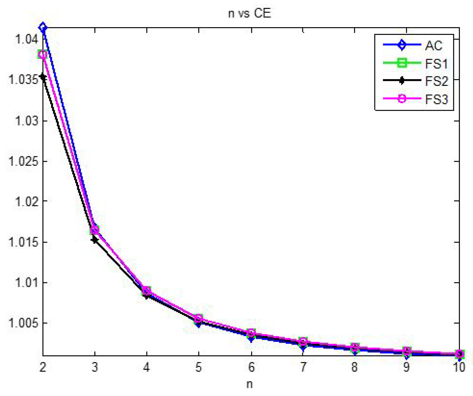
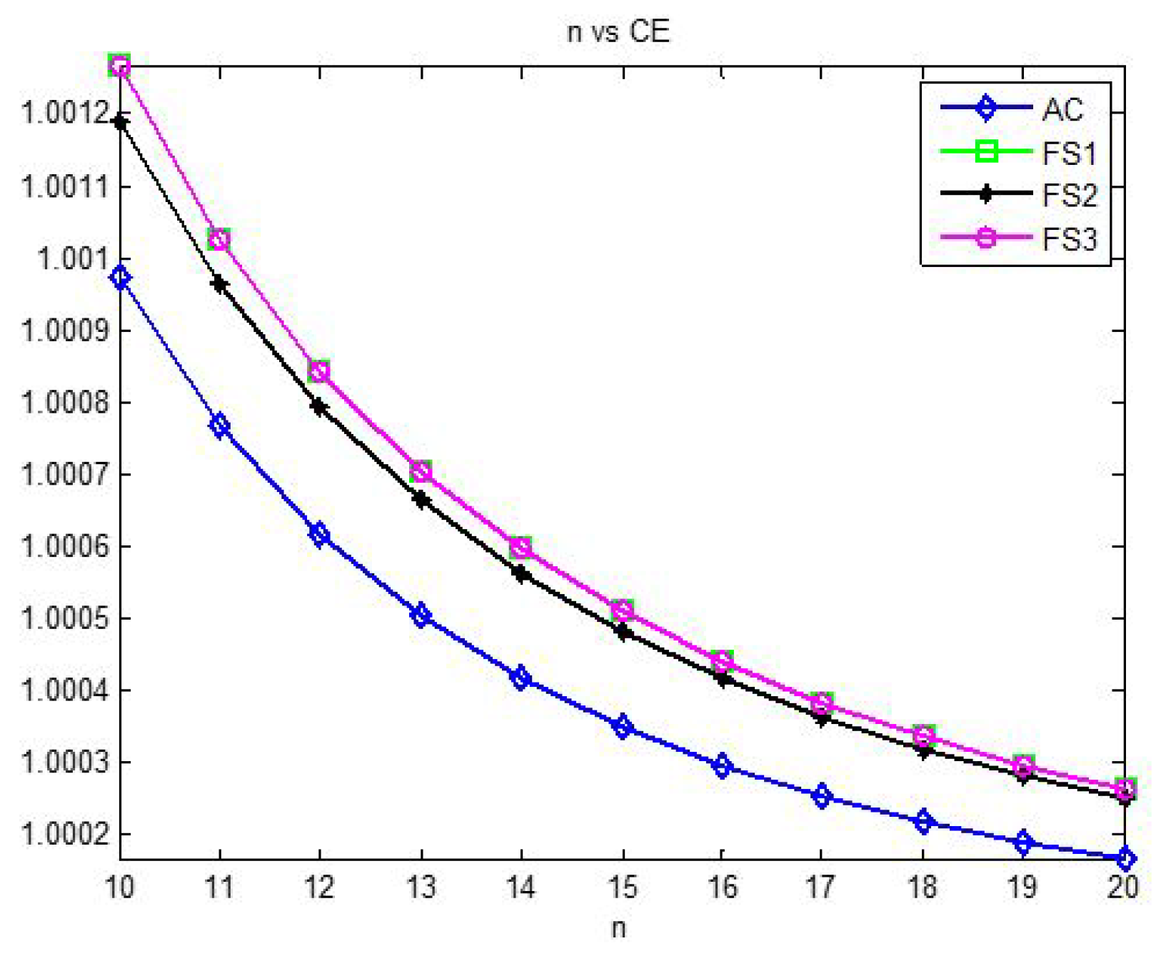
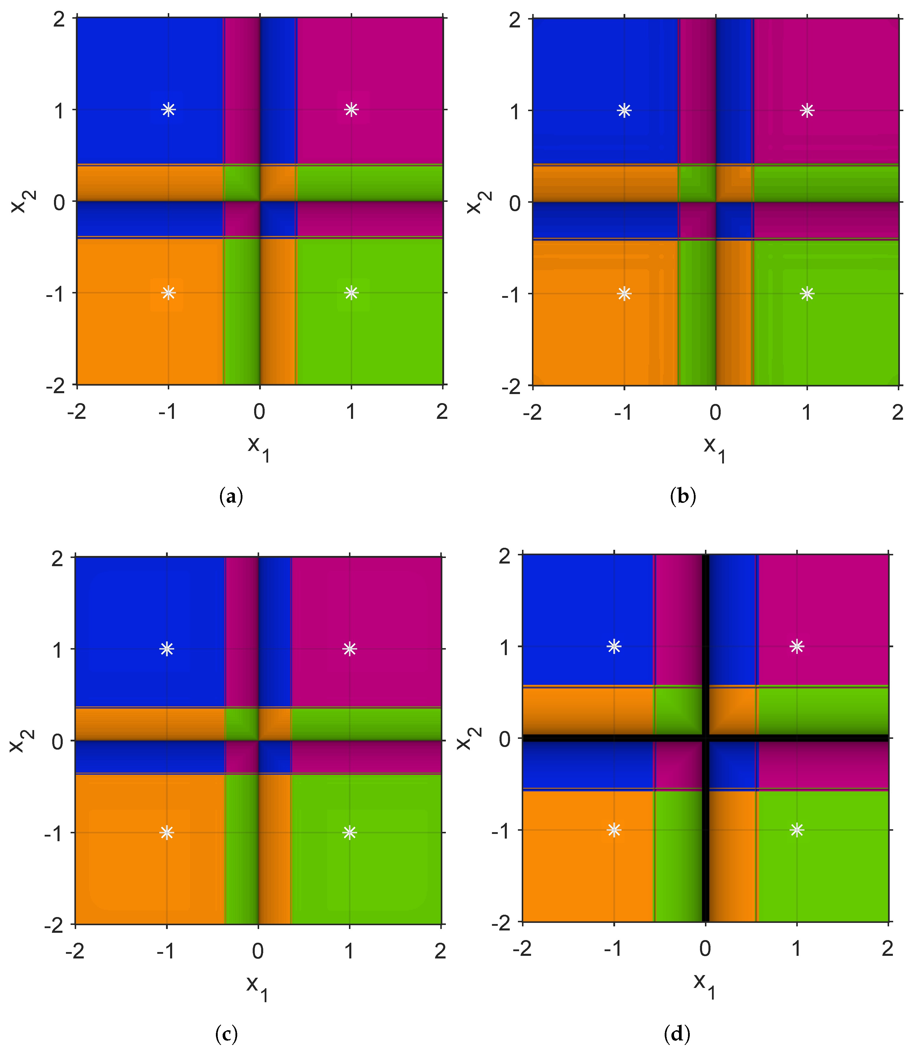
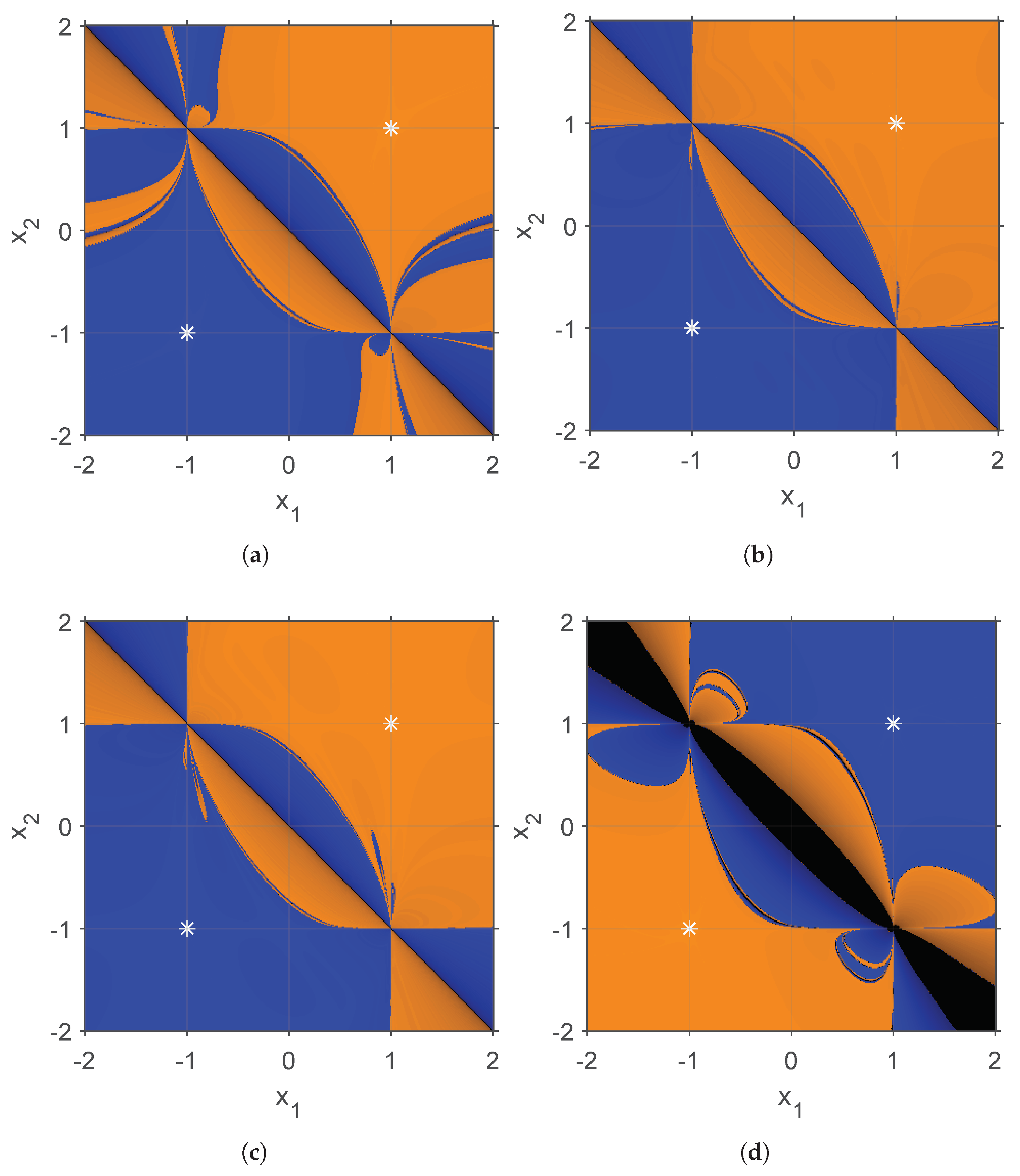
3. Numerical Results

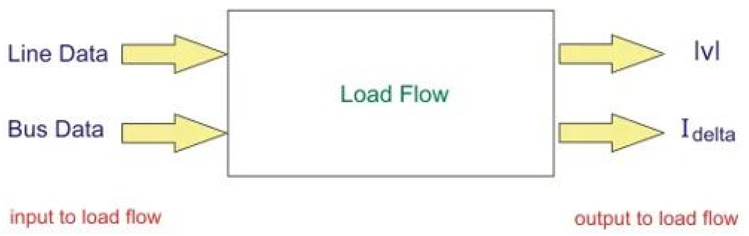
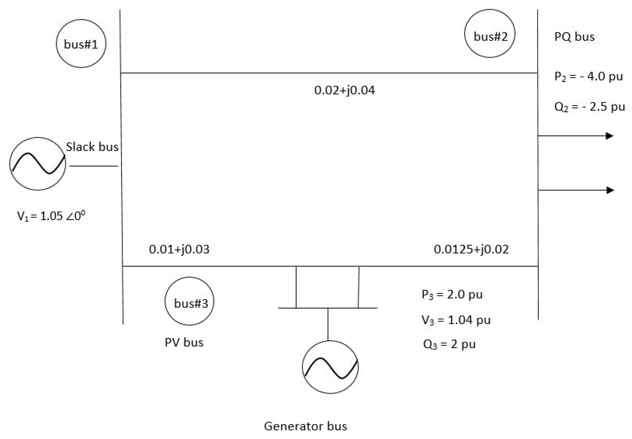
3.1. Equations for Load Flow Analysis

The traditional power flow equation is defined in terms of real power $\left(P\right)$, reactive power $\left(Q\right)$ and voltage $\left(V\right)$ as:

$$R_i=P_i+j{Q}_i,$$

where $P_i$ is the real power injection (positive) or withdrawal (negative) at bus $n,Q_i$ is the reactive power injection or withdrawal at bus n and $R_i$ is the net complex power injection.

$$R_i=V_i{I}^{*}=V_i{(\sum _{k=1}^n{Y}_{ik}{V}_k)}^{*},$$

so the power injections can be written as,

$$R_i^{*}=P_i-j{Q}_i=V_i^{*}I=V_i^{*}\sum _{k=1}^n{Y}_{ik}{V}_k.$$

The transformation from rectangular to polar coordinates for the complex voltage is given as:

$$V_i=|V_i|\angle {\delta }_i,V_k=|V_k|\angle {\delta }_k,Y_{ik}=\left|Y_{ik}\right|\angle {\theta }_{ik},$$

Hence,

$$R_i^{*}=P_i-j{Q}_i=\left(\right|V_i|\angle -{\delta }_i)\sum _{k=1}^n\left(\right|Y_{ik}|\angle {\theta }_{ik}\left)\right(|V_k|\angle {\delta }_k),$$

$$R_i^{*}=\sum _{k=1}^n\left|Y_{ik}{V}_k{V}_i\right|\angle ({\theta }_{ik}+{\delta }_k-{\delta }_i),$$

where $\theta$ be the voltage angle and $\delta$ be the current angle. Now separating real and imaginary components, we obtain the equations for real and reactive power as follows:

$$P_i=|V_i|\sum _{k=1}^n\left|Y_{ik}{V}_k\right|cos({\theta }_{ik}+{\delta }_k-{\delta }_i),$$

(15)

and

$$Q_i=-|V_i|\sum _{k=1}^n\left|Y_{ik}{V}_k\right|sin({\theta }_{ik}+{\delta }_k-{\delta }_i).$$

(16)

Now, we want to verify the numerical results of our iterative method so, we consider the power flow problem and compare the numerical results of our scheme namely $F{S}_1$, $F{S}_2$ and $F{S}_3$ with respect to the number of iterations m, the absolute residual error of the corresponding function $∥G\left(r^{\left(m\right)}\right)∥$, absolute error in two consecutive iterations $∥r^{\left(m\right)}-r^{(m-1)}∥$ and computational order of convergence [23] expressed as $\delta \approx \frac{ln\left(\frac{∥G\left(r^{(m+1)}\right)∥}{∥G\left(r^{\left(m\right)}\right)∥}\right)}{ln\left(\frac{∥G\left(r^{\left(m\right)}\right)∥}{∥G\left(r^{(m-1)}\right)∥}\right)}$. All numerical results are obtained by using Maple 13 in a PC with specifications: Intel(R) Core(TM) i5 CPU 6300U @ 2.40 GHz, 2.50 GHz (64-bit Operating System) Microsoft Windows 10 Professional and 8 GB RAM with a precision of 300 digits. We compare our method with the seventh-order method presented by Abad et al. [17] named as AC.

Example 1. 

Let us consider 3 bus power system with the generator at bus 1 and bus 3 where the unit for measurement is per-unit (p.u.). The magnitude of the voltage at bus1 is adjusted to 1.05 pu. Voltage magnitude at bus 3 is fixed at 1.04 pu with a real power generation of 2.0 pu. A load consisting of $-4.0$ pu and $-2.5$ pu is taken from bus 2. Line impedances can be shown in Figure 4.

As the numbers of buses are three so, $Y_{bus}$ can be written as:

$Y_{bus}$$=\left[\begin{array}{ccc}{Y}_{11}& Y_{12}& Y_{13}\\ Y_{21}& Y_{22}& Y_{23}\\ Y_{31}& Y_{32}& Y_{33}\end{array}\right]=\left[\begin{array}{ccc}53.851\angle -68.{198}^0& 22.360\angle 116.{56}^0& 31.6228\angle 108.{434}^0\\ 22.360\angle 116.{56}^0& 58.137\angle -63.{434}^0& 35.777\angle 116.{565}^0\\ 31.6228\angle 108.{434}^0& 35.777\angle 116.{565}^0& 67.2309\angle -67.{249}^0\end{array}\right]$

By expanding (15) and (16) we get:

$$\begin{array}{c}\hfill P_2=V_2\sum _{k=1}^3{Y}_{2k}{V}_{k}cos({\theta }_{2k}+{\delta }_k-{\delta }_2),\end{array}$$

(17)

$$\begin{array}{c}\hfill P_3=V_3\sum _{k=1}^3{Y}_{3k}{V}_{k}cos({\theta }_{3k}+{\delta }_k-{\delta }_3),\end{array}$$

(18)

$$\begin{array}{c}\hfill Q_2=-V_2\sum _{k=1}^3{Y}_{2k}{V}_{k}sin({\theta }_{2k}+{\delta }_k-{\delta }_2).\end{array}$$

(19)

After substituting values of $Y_{bus}$ in (17)–(19) we get a system of three nonlinear equations with three unknowns given as:

$$\begin{array}{ccc}\hfill P_2& =& 23.478630V_{2}cos(-2.0344+{\delta }_2)+26.00005V_2^2\hfill \\ \hfill & & +37.20818V_{2}cos(-2.0344-{\delta }_3+{\delta }_2)+4,\hfill \\ \hfill P_3& =& 34.53209cos(-1.89254+{\delta }_3)+37.208184V_{2}cos(2.034444788+{\delta }_2-{\delta }_3)\hfill \\ \hfill & & +26.12160874,\hfill \\ \hfill Q_2& =& 23.47863V_{2}sin(-2.03444+{\delta }_2)+52.0000V_2^2\hfill \\ \hfill & & +37.20818V_{2}sin(-2.034444788-{\delta }_3+{\delta }_2)+2.5.\hfill \end{array}$$

The value $r^{\left(0\right)}={(0,0,1)}^t$ is taken as the initial value and the solution of the nonlinear system for the given problem is $\mathsf{{\rm Y}}={(-0.047062483774,-0.00870636568,0.971677789143)}^t.$

Remark 1. 

We have calculated the voltage magnitude and phase angles of the three-bus power system with greater accuracy. The efficiency index (I) and computational efficiency index (CI) [22] of the above example indicate that the four methods present an efficiency index of I = 7${}^{(1/30)}$. However, they have marginal differences in the computational efficiency indexes, with values 7${}^{(1/117)}$, 7${}^{(1/119)}$ and 7${}^{(1/128)}$ for the AC, FS${}_1$-FS${}_3$ and FS${}_2$ methods, respectively. However, these small differences are reflected in the accuracy of the results as evident from

Table 3. Comparison of methods for the load flow problem.

$\mathbf{Cases}$	m	${\Vert {\mathit{r}}^{\left(\mathit{m}\right)}-{\mathit{r}}^{(\mathit{m}-1)}\Vert }_{\mathit{\infty }}$	$\Vert \mathit{G}\left({\mathit{r}}^{\left(\mathit{m}\right)}\right){\Vert }_{\mathit{\infty }}$	$\mathit{\delta }$
$F{S}_1$	1	$4.706246e(-2)$	$1.464301e(-6)$	−
	2	$2.639187e(-8)$	$1.199179e(-38)$	$5.10062$
	3	$1.665677e(-40)$	$4.493960e(-198)$	$7.33718$
${FS}_2$	1	$4.706248e(-2)$	$7.325844e(-7)$	−
	2	$2.713283e(-8)$	$2.067714e(-38)$	$4.78636$
	3	$6.219538e(-40)$	$1.170039e(-196)$	$7.42478$
$F{S}_3$	1	$4.706248e(-2)$	$1.539407e(-6)$	−
	2	$2.497081e(-8)$	$2.147565e(-37)$	$4.92188$
	3	$3.587427e(-39)$	$5.018327e(-192)$	$7.40976$
$AC$	1	$4.706248e(-2)$	$2.850094e(-6)$	−
	2	$3.482259e(-8)$	$1.527893e(-36)$	$5.04385$
	3	$2.406074e(-38)$	$1.218126e(-187)$	$7.37009$

.

3.2. Stability of the Methods

The iterative methods under study will be employed to solve two academic nonlinear systems with the objective of analyzing the proximity of the initial estimate to the solution. In this regard, their corresponding dynamical planes are represented.

Dynamical planes are commonly used to analyze the stability of a method. To solve nonlinear equations, a set of initial estimates $z_0\in \widehat{\mathbb{C}}$ is selected, representing the real and imaginary parts of $z_0$ on the abscissae and ordinates, respectively. Each root is assigned a color, and each initial point is represented by the color to whose root it converges. To solve nonlinear systems of two equations, a set of initial guesses $x^{\left(0\right)}={\left(\begin{array}{c}{x}_1\\ x_2\end{array}\right)}^{\left(0\right)}$ is selected, and the representation follows the same rules as in the case of nonlinear equations.

A set of 400 equally spaced initial estimates in the square $\{x^{\left(0\right)}\in {\mathbb{R}}^2:-2\le x_1,x_2\le 2\}$ is taken. The convergence is set when $\parallel x^{(k+1)}-x^{\left(k\right)}\parallel <{10}^{-6}$. If this condition is not achieved after 50 iterations, divergence is interpreted. The information about the number of iterations is also included by scaling the brightness of the points: the darkest scaling, the most number of iterations. The roots of the nonlinear system of equations are represented with white stars. The generation of the dynamical planes follows the guidelines given in [24].

The discussion begins with the uncoupled system of nonlinear equations

$$\left\{\begin{array}{c}{x}_1^2-1=0,\hfill \\ x_2^2-1=0,\hfill \end{array}\right.$$

(20)

whose solutions are $(1,1)$, $(1,-1)$, $(-1,-1)$, and $(-1,1)$. Purple, green, orange and blue colors represent the initial points whose orbit converges to the roots $(1,1)$, $(1,-1)$, $(-1,-1)$, and $(-1,1)$, respectively. Black color represents divergence, and white stars represent the roots. Figure 5 collects the dynamical planes of the methods AC, FS1, FS2 and FS3.

Global convergence can be observed at Figure 5 applying methods AC, FS1 and FS2, with slower convergence for those initial guesses that are close to the axis. Method FS3 has wide convergence except for initial guesses that are close to the axis, since the denominators are very close to zero at these points.

The second system of nonlinear equations to discuss is

$$\left\{\begin{array}{c}{x}_1{x}_2+x_1-x_2-1=0,\hfill \\ x_1{x}_2-x_1+x_2-1=0,\hfill \end{array}\right.$$

(21)

whose solutions are $(1,1)$, and $(-1,-1)$. Blue and orange colors represent the initial points whose orbit converges to the roots $(1,1)$, and $(-1,-1)$, respectively. Black color represents divergence, and white stars represent the roots. Figure 6 collects the dynamical planes of the methods AC, FS1, FS2 and FS3.

Global convergence can be again observed at Figure 6 applying methods AC, FS1 and FS2, but the line $x_1+x_2=0$. This band is broader in method FS3. The darkness of this line is caused by the proximity of the denominator operator to zero, leading to regions of slow convergence or even divergence. The basins of attraction of Figure 6b,c are less intricate than Figure 6a, improving the stability of methods FS1 and FS2 with respect to AC.

Let us remark that both FS1 and FS2 methods allow using values of the initial estimate more distant from the solution.

4. Conclusions

We developed a new seventh-order scheme for a solving nonlinear system of equations using weight functions. We analyzed a power flow problem and calculated phase angle and voltage magnitude using the new schemes. Numerical results of the power flow-based problem are further supported when we compare our scheme with existing families of the same domain [17]. In addition, methods FS1 and FS2 show global convergence, allowing initial guesses further away from the solution.

References

1. Moré, J.J. A collection of nonlinear model problems. In Computational Solution of Nonlinear Systems of Equations, Lectures in Applied Mathematics; Allgower, E.L., Georg, K., Eds.; American Mathematical Society: Providence, RI, USA, 1990; Volume 26, pp. 723–762. [Google Scholar]
2. Grosan, C.; Abraham, A. A new approach for solving nonlinear equations systems. IEEE Trans. Syst. Man Cybernet Part A Syst. Humans 2008, 38, 698–714. [Google Scholar] [CrossRef]
3. Lin, Y.; Bao, L.; Jia, X. Convergence analysis of a variant of the newton method for solving nonlinear equations. Comput. Math. Appl. 2010, 59, 2121–2127. [Google Scholar] [CrossRef] [Green Version]
4. Ward, J.B.; Hale, H.W. Digital computer solution of power flow problems. AIEE Trans. 1956, 75, 398–404. [Google Scholar]
5. Iwamoto, S.; Tamura, Y. Load flow calculation method for ill-conditioned power systems. IEEE Trans. Power Appar. Syst. 1981, 100, 1736–1743. [Google Scholar] [CrossRef]
6. Stott, B. Review of load-flow calculation methods. Proc. IEEE 1974, 62, 916–929. [Google Scholar] [CrossRef]
7. Tinney, W.F.; Hart, C.E. Power flow solution by Newton’s method. IEEE Trans. Power Appar. Syst. 1967, PAS-86, 1449–1460. [Google Scholar] [CrossRef]
8. Stott, B.; Alsac, O. Fast decoupled load flow. IEEE Trans. Power Appar. Syst. 1974, PAS-93, 859–869. [Google Scholar] [CrossRef]
9. Changbum, C.; Neta, B. A third-order modification of Newton’s method for multiple roots. Appl. Math. Comput. 2009, 211, 474–479. [Google Scholar]
10. Dzunic, J.; Petkovic, M.S. A family of three-point methods of Ostrowski’s type for solving nonlinear equations. J. Appl. Math. 2012, 2012, 425867. [Google Scholar] [CrossRef] [Green Version]
11. Soleymani, F.; Vanani, S.K. Numerical solution of nonlinear equations by an optimal eighth-order class of iterative methods. Ann. Univ. Ferrara 2013, 59, 159–171. [Google Scholar] [CrossRef]
12. Behl, R.; Argyros, I.K. A new higher order iterative scheme for the solutions of nonlinear systems. Mathematics 2020, 8, 271. [Google Scholar] [CrossRef] [Green Version]
13. Behl, R.; Sarría, I.; González, R.; Magreñán, A.A. Highly efficient family of iterative methods for solving nonlinear models. J. Comput. Appl. Math. 2019, 346, 110–132. [Google Scholar] [CrossRef]
14. Kansal, M.; Cordero, A.; Bhalla, S.; Torregrosa, J.R. New fourth and sixth-order classes of iterative methods for solving systems of nonlinear equations and their stability analysis. Numer. Algor. 2021, 87, 1017–1060. [Google Scholar] [CrossRef]
15. Lee, M.Y.; Kim, Y.I. Development of a family of Jarratt-like sixth-order iterative methods for solving nonlinear systems with their basins of attraction. Algorithms 2020, 13, 303. [Google Scholar] [CrossRef]
16. Amiri, A.; Cordero, A.; Darvishi, M.T.; Torregrosa, J.R. Stability analysis of a parametric family of seventh-order iterative methods for solving nonlinear systems. Appl. Math. Comput. 2018, 323, 43–57. [Google Scholar] [CrossRef]
17. Abad, M.; Cordero, A.; Torregrosa, J.R. A family of seventh order schemes for solving nonlinear systems. Bull. Math. Soc. Sci. Math. Roum. Tome 2014, 57, 133–145. [Google Scholar]
18. Behl, R.; Arora, H. A novel scheme having seventh-order convergence for nonlinear systems. J. Comput. Appl. Math. 2022, 404, 113301. [Google Scholar] [CrossRef]
19. Grau-Sánchez, M.; Noguera, M.; Amat, S. On the approximation of derivatives using divided difference operators preserving the local convergence order of iterative methods. J. Comput. Appl. Math. 2013, 237, 363–372. [Google Scholar] [CrossRef]
20. Moysi, A.; Ezquerro, J.A.; Hernández-Verón, M.Á.; Magreñán, Á.A. On the set of initial guesses for the secant method. Math. Meth. Appl. Sci. 2023, 2023, 1–14. [Google Scholar] [CrossRef]
21. Ortega, J.M.; Rheinboldt, W.G. Iterative Solutions of Nonlinear Equations in Several Variables; Academic Press: New York, NY, USA, 1970. [Google Scholar]
22. Cordero, A.; Torregrosa, J.R. On interpolation variants of Newton’s method for functions of several variables. J. Comput. Appl. Math. 2010, 234, 34–43. [Google Scholar] [CrossRef] [Green Version]
23. Soleymani, F.; Sharifi, M.; Shateyi, S.; Haghani, F.K. Iterative methods for nonlinear equations or systems and their applications. J. Appl. Math. 2014, 2014, 705375. [Google Scholar] [CrossRef]
24. Chicharro, F.I.; Cordero, A.; Torregrosa, J.R. Drawing dynamical and parameters planes of iterative families and methods. Sci. World J. 2013, 780153. [Google Scholar] [CrossRef] [PubMed] [Green Version]
Figure 1. Schematic of the power flow problem.
Fractalfract 07 00317 g001
Figure 2. Comparison of Computational Efficiency for 2 n 10 .
Fractalfract 07 00317 g002
Figure 3. Comparison of Computational Efficiency for 10 n 20 .
Fractalfract 07 00317 g003
Figure 4. Power System.
Fractalfract 07 00317 g004
Figure 5. Dynamical planes of solving system (20) with the methods (a) AC, (b) FS1, (c) FS2, and (d) FS3.
Fractalfract 07 00317 g005
Figure 6. Dynamical planes of solving system (21) with the methods (a) AC, (b) FS1, (c) FS2, and (d) FS3.
Fractalfract 07 00317 g006