Article

Sequential Predictors for Uncertain Euler–Lagrange Systems with Large Transmission Delays

1
School of Microelectronics and Control Engineering, Changzhou University, Changzhou 213164, China
2
School of Automation and Electrical Engineering, Linyi University, Linyi 276000, China
3
School of Instrument Science and Engineering, Southeast University, Nanjing 210096, China
4
School of Automation Engineering, Nanjing University of Aeronautics and Astronautics, Nanjing 211106, China
*
Author to whom correspondence should be addressed.
Fractal Fract. 2023, 7(3), 244; https://doi.org/10.3390/fractalfract7030244
Submission received: 3 January 2023 / Revised: 6 March 2023 / Accepted: 7 March 2023 / Published: 8 March 2023

Abstract

:
This paper investigates the state prediction problems for uncertain Euler–Lagrange systems with large time delays during data transmissions. A set of sequential predictors is proposed to estimate the actual real-time states of the systems by using the delayed information of measurements. The arbitrarily large delays are handled by applying adequate numbers of serial sub-predictors. Meanwhile, the novel prediction structure of each subsystem is designed to deal with nonlinearities and unknown dynamics in the systems. Then, the predictor design is extended to the case without using delayed velocity measurements by updating the structure of the first sub-predictor. Sufficient conditions for the design of predictor gains, ensuring the boundness of prediction errors, are obtained through Lyapunov–Krasovskii functionals. The effectiveness and robustness of the uncertainties of the proposed method are verified by comparative results in simulations.

1. Introduction

Time delays have attracted great attentions in the design of control systems with the development of Internet technology over the recent two decades [1,2,3,4,5]. Since the large transmission delays are unavoidable in long-distance sensor and communication networks, they badly damage the performance of remotely controlled system [6,7], such as in robotic systems [8], multiagent systems [9], and network systems [10]. Though a large amount of control and estimation techniques have been proposed to deal with time delays in the state variables or inputs [11,12,13,14], only a few results are available for systems with delayed output measurements. Especially for relatively large communication delays, the predictor design based on the delayed outputs remains an open problem.
Numerous control and state prediction methods have been proposed for linear systems with time delay, such as the famous Smith predictor [15] and Artstein reduction model [16]. In [17], a nonlinear version of the Smith predictor is proposed for forward complete nonlinear systems. Then, this approach is extended to multi-input systems [18], Euler–Lagrange systems [19], and the cases of distributed unbounded input delays [20,21], respectively. In [22], the reduction model is developed with nonlinear systems to compensate the input delays. Though these mentioned methods are able to deal with delays with arbitrary sizes, they are sensitive to noises and uncertainties, due to the open-loop structure of predictors. Recently, several observer-based prediction methods were proposed to estimate the actual state of nonlinear systems by using delayed outputs. For examples, high gain predictors were applied to nonlinear systems for state estimation and controller design in [23,24,25]. In [26,27], predictor-based continuous-discrete observers were designed for systems with delayed and sampled outputs. However, these observer-based predictors can only deal with relatively small delays.
Sequential predictor approaches were introduced by using several interconnected observer-based sub-predictors [28,29,30]. Each sub-predictor provides a prediction of the output state of the previous one in a small prediction horizon, such that arbitrarily long input/output delays can be compensated through applying sufficient numbers of sub-predictors. In [29,30,31], sequential predictors were proposed to reconstruct the states of nonlinear systems with constant measurement delays. An output reconstruction method was proposed in [32] to deal with time-varying delays by intentionally further delaying the original outputs. Moreover, the designs of sequential predictors in cases of sampled measurements [33,34] and discrete nonlinear systems [35] were successively studied. Nevertheless, the above-mentioned predictors were designed based on the assumptions of Lipschitz conditions for nonlinearities, which are not suitable for general Euler–Lagrange systems.
Motivated by recent studies on predictive controller design methods for nonlinear systems in [36,37,38], this paper presents a new prediction approach for a class of uncertain Euler–Lagrange systems subject to large transmission delays, which can be applied to robotic and other mechanical systems [39,40]. Through applying adequate sub-predictors, the arbitrary large output delay can be handled by the designed sequential predictor. Meanwhile, novel prediction algorithms of sub-predictors are proposed to deal with the nonlinearities and uncertainties in the Euler–Lagrange system. The boundness of prediction errors can be verified by using Lyapunov–Krasovskii functionals. In addition, the velocity-free case is considered in this paper. By updating the structure of the first sub-predictor, the actual states of the system can be estimated by the proposed sequential predictor by using only the delayed position measurements. The main contributions and novelties of this paper are summarized as follows:
1. Three major problems during the state estimation, including large output delay, nonlinearity, and uncertainty, are addressed simultaneously by the proposed sequential predictor. In particular, different from the previous works in [29,30,31,32], the prediction method in this paper is designed specially for Euler–Lagrange systems, which does not need the nonlinearities in the systems to satisfy the Lipschitz condition.
2. A simple modified prediction method is proposed to extend the predictor design to the velocity-free case. Compared with previous studies, where observers are applied in front of the cascade sub-predictors to estimate the delayed velocities [40,41,42], the updated sequential predictor is easier to implement, and the prediction results will not be affected by the observation error.
The rest of this paper is organized as follows. In Section 2, some preliminary and problem statements are illustrated. Then, the sequential predictor design using both delayed position and velocity measurements is presented in Section 3. Additionally, the prediction method is extended to the velocity-free case in Section 4. Next, the simulation results are given in Section 5 to show the effectiveness of the proposed approaches. Finally, Section 6 summarizes this paper.

2. Preliminaries and Problem Statement

Consider a class of an uncertain Euler–Lagrange system with transmission delay, which is described as follows:
x ˙ 1 ( t ) = x 2 ( t ) , M ( x 1 ) x ˙ 2 ( t ) + C ( x 1 , x 2 ) x 2 ( t ) = F ( x 1 , x 2 , u , t ) , y ( t ) = x ( t τ ) , t [ t 0 , ) .
with any initial conditions
x ( t ) = x 0 ( t ) , t [ t 0 τ , t 0 ] .
where x ( t ) = [ x 1 ( t ) T x 2 ( t ) T ] T represents the state variable, x 1 ( t ) and x 2 ( t ) n are the joint positions and velocities, respectively, M ( x 1 ) n × n is a positive definite inertia matrix, C i ( x 1 , x 2 ) n × n is the matrix of the centripetal and coriolis torques, and F ( x 1 , x 2 , u , t ) is an uncertain function containing unknown dynamics and input. y ( t ) = [ y 1 ( t ) T y 2 ( t ) T ] T is the delayed output with a constant time delay τ , where y 1 ( t ) = x 1 ( t τ ) and y 2 ( t ) = x 2 ( t τ ) .
As is mentioned in the Introduction, the first objective of this paper is to design a sequential predictor that renders an estimation of the actual state x ( t ) by using the delayed outputs y ( t ) . Then, the proposed method is extended to the case, without applying velocity measurements y 2 ( t ) . Two main challenges shall be addressed when designing the predictor. The first one is the large transmission delay in the output and the second deals with the nonlinearities and uncertainties in the Euler–Lagrange system.
The following common assumptions are useful during the predictor design:
Assumption A1
([43]). The inertia matrix M i ( q i ) is positive definite and satisfies λ 1 I M ( x 1 ) λ 2 I , where λ 1 and λ 2 are positive constants.
Assumption A2.
The state variable x ( t ) is bounded.
Assumption A3.
The unknown function F ( x 1 , x 2 , u , t ) is bounded when x ( t ) is bounded, and there is a known constant d ¯ , such that
| | F ( x 1 , x 2 , u , t ) | | d ¯ .
where | | · | | represents the standard Euclidean norm.
Remark 1.
Assumptions 2 and 3 are commonly used when designing the predictors and controllers, such as in [37,38].

3. Sequential Predictor Design Using Both Delayed Position and Velocity Measurements

3.1. Construction of Sequential Predictor

In the case that both the delayed position and velocity measurements are available, the proposed sequential predictor for system (1) is formed by several sub-predictors in series, which is given by the following set of equations, for i = 1 , 2 , , m , and t t 0 :
x ^ ˙ 1 i ( t ) = x ^ 2 i ( t ) M ( x ^ 1 i ( t ) ) x ^ ˙ 2 i ( t ) = C ( x ^ 1 i ( t ) , x ^ 2 i ( t ) ) x ^ 2 i ( t ) + k r τ i ( t )
where m 1 is the number of sub-predictors, x ^ i = [ x ^ 1 i T x ^ 2 i T ] T represents the predicted state variable of each sub-predictor, k = k a + k b + k c + k d is the positive predictor gain, k a , k b , k c , k d are auxiliary positive predictor gains, and r τ i ( t ) is the term of error feedback, which is formulated as:
for i = 1 ,
r τ 1 ( t ) = α ( y 1 ( t ) x ^ 11 ( t τ m ) ) + y 2 ( t ) x ^ 21 ( t τ m ) M 1 ( x ^ 1 i ( t τ m ) ) θ τ 1 ( t ) ;
for 2 i m ,
r τ i ( t ) = α ( x ^ 1 , i 1 ( t ) x ^ 1 i ( t τ m ) ) + x ^ 2 , i 1 ( t ) x ^ 2 i ( t τ m ) M 1 ( x ^ 1 i ( t τ m ) ) θ τ i ( t ) ,
where α is a positive constant gain, and
θ τ i ( t ) = t τ / m t k r τ i ( σ ) d σ , i = 1 , , m .
The actual state of x ( t ) is estimated by the last sub-predictors, i.e., x ^ m ( t ) = [ x ^ ˙ 1 m T ( t ) x ^ ˙ 2 m T ( t ) ] T . The prediction errors are defined as
e 1 i ( t ) = x 1 i ( t ) x ^ 1 i ( t ) , e 2 i ( t ) = x 2 i ( t ) x ^ 2 i ( t ) ,
where x i ( t ) = [ x 1 i T ( t ) x 2 i T ( t ) ] T is defined as [30]:
x 1 i ( t ) = x 1 ( t τ + i m τ ) , x 2 i ( t ) = x 2 ( t τ + i m τ ) .
Obviously, there is x i = m ( t ) = x ( t ) . Additionally, the following relationship is satisfied:
x i ( t τ m ) = x i 1 ( t ) , i 2 .
Actually, from (5) and (6), each sub-predictor provides an estimation of x i ( t ) through predicting x ^ i 1 ( t ) (or y ( t ) when i = 1 ) in a time horizon τ / m .

3.2. Convergence Analysis of Prediction Errors

Consider the following auxiliary error variables
r i ( t τ m ) = r τ i ( t ) ,
θ i ( t ) = t τ m t k r i ( σ ) d σ ,
R i ( t ) = e 2 i ( t ) + α e 1 i ( t ) M 1 ( x ^ 1 i ( t ) ) θ i ( t ) .
By using the relationship (10), it can be obtained from Equations (5)–(7) and (11)–(13) that
R 1 ( t τ m ) = r 1 ( t τ m ) ,
and for 2 i m ,
R i ( t τ m ) = r i ( t τ m ) + e 2 , i 1 ( t ) + α e 1 , i 1 ( t ) .
After defining
e 1 , 0 ( t ) = e 2 , 0 ( t ) = 0 ,
it can be concluded from Equations (14) and (15) that
R i ( t ) = r i ( t ) + E i 1 ( t ) , i = 1 , 2 , , m ,
where E i 1 ( t ) = e 2 , i 1 ( t + τ / m ) + α e 1 , i 1 ( t + τ / m ) .
Subsequently, through taking the time derivative of R i ( t ) in (13) and multiplying both sides by M ( x ^ 1 i ( t ) ) , the closed-loop prediction error system can be presented as follows (the time argument t is omitted for brevity):
M ( x ^ 1 i ) R ˙ i = M ( x ^ 1 i ) [ x ˙ 2 i x ^ ˙ 2 i + α e 2 i ] + M 1 ( x ^ 1 i ) θ i + k ( r τ i r i ) = f ˜ i 1 2 M ˙ ( x ^ 1 i ) x ^ 2 i R i e 1 i + F k R i k E i 1 ,
where i = 1 , 2 , , m , the auxiliary term f ˜ i ( t ) is defined as
f ˜ i ( t ) = M ( x ^ 1 i ) [ M 1 ( x 1 i ) C ( x 1 i , x 2 i ) x 2 i + M 1 ( x ^ 1 i ) C ( x ^ 1 i , x ^ 2 i ) x ^ 2 i ] + α M ( x ^ 1 i ) ( R i α e 1 i + M ( x ^ 1 i ) 1 θ i ) + M 1 ( x ^ 1 i ) θ i + 1 2 M ˙ ( x ^ 1 i ) x ^ 2 i R i + e 1 i .
Similar to [43,44], the mean value theorem is utilized into the expression in (19) to obtain the upper bound of f ˜ i ( t ) as
| | f ˜ i ( t ) | | ρ ( | | z i ( t ) | | ) | | z i ( t ) | | ,
where ρ ( · ) is a positive and non-decreasing function, z i 3 n is defined as
z i ( t ) = e 1 i T ( t ) R i T ( t ) θ i T ( t ) T .
Theorem 1.
Consider system (1) subject to Assumptions 1–3 and sequential predictor (4)–(7). If both the number of sub-predictors m and the predictor gain k are designed to be sufficiently large, relative to the initial conditions of the system, then the prediction errors e 1 i ( t ) and e 2 i ( t ) converge to the bounded regions. More precisely, if the following conditions are simultaneously fulfilled for all i = 1 , 2 , , m :
m > k 2 ( λ 1 2 + 2 ) 2 κ 1 δ τ ,
α > δ 2 , δ < 2 ,
k a > 0 , k b > ρ 2 ( | | z i ( t 0 ) | | ) 4 s 1 ( 1 δ 2 ) , k c > δ + 2 κ 2 + 2 κ 1 τ m 1 δ 2 , k d > 0 .
then there exists positive constants ϵ 0 , ϵ 1 and ϵ 2 i such that for all i = 1 , 2 , , m ,
| | e 1 i ( t ) | | ϵ 0 e ϵ 1 t + ϵ 2 i ,
where δ, κ 1 , κ 2 are some arbitrarily designed positive constants, and
s 1 = min α δ 2 , ( 1 δ 2 ) k a , κ 1 m k 2 τ λ 1 2 + 2 2 δ .
Proof of Theorem 1.
For the brevity of subsequent analysis, the time argument t is omitted throughout this proof.
Consider the following Lyapunov–Krasovskii functional for i = 1 , 2 , , m :
V i = 1 2 e 1 i T e 1 i + 1 2 R i T M ( x ^ 1 i ) R i + 1 2 k θ i T θ i + Q i + P i ,
where Q i , P i n are given as
Q i = κ 1 t τ / m t s t | | r i ( σ ) | | 2 d σ d s ,
P i = κ 2 t τ / m t | | r i ( σ ) | | 2 d σ .
Based on Assumption 1, V i is bounded by
c 1 | | w i | | 2 V i ( y , t ) c 2 | | w i | | 2 .
where c 1 = m i n 1 2 , 1 2 λ 1 , 1 2 k , and c 2 = m a x 1 , 1 2 λ 2 , 1 2 k , and w i 5 n is defined as
w i = e 1 i T R i T θ i T Q i P i T ,
Utilizing Equations (12), (13), and (18), the time derivative of V i can be calculated as:
V ˙ i = e 1 i T ( R i α e 1 i M 1 θ i ) + R i T ( f ˜ i e 1 i + F k ( R i E i 1 ) ) + θ i T ( r τ i r i ) + Q ˙ i + P ˙ i = α | | e 1 i | | 2 e 1 i T M 1 θ i + R i T ( f ˜ i + F ) + k R i T E i 1 k | | R i | | 2 + θ i T ( r τ i r i ) + κ 1 τ m | | r i | | 2 κ 1 t τ / m t | | r i ( σ ) | | 2 d σ + κ 2 ( | | r i | | 2 | | r τ i | | 2 ) .
By applying Assumption 1–3, and the following general Young’s inequality
| | a b | | δ 2 | | a | | 2 + 1 2 δ | | b | | 2 ,
V ˙ i in the expression (32) can be upper bounded as:
V ˙ i ( α δ 2 ) | | e 1 i | | 2 ( 1 δ 2 ) k | | R i | | 2 + | | R i | | ρ ( | | z i | | ) | | z i | | + | | R i | | d ¯ + k 2 δ | | E i 1 | | 2 ( κ 2 δ 2 ) | | r τ i | | 2 + ( δ 2 + κ 2 + κ 1 τ m ) | | r i | | 2 + λ 1 2 + 2 2 δ | | θ i | | 2 κ 1 t τ / m t | | r i ( σ ) | | 2 d σ
Based on (12), the Cauchy–Schwarz inequality is used to derive the upper bound of | | θ i | | 2 , as in [44]
| | θ i | | 2 k 2 τ m t τ / m t | | r i ( σ ) | | 2 d σ .
Thus, V ˙ i can be further upper bounded as
V ˙ i ( α δ 2 ) | | e 1 i | | 2 ( 1 δ 2 ) k | | R i | | 2 + | | R i | | ρ ( | | z i | | ) | | z i | | + | | R i | | d ¯ + k 2 δ | | E i 1 | | 2 ( κ 2 δ 2 ) | | r τ i | | 2 + ( δ 2 + κ 2 + κ 1 τ m ) | | r i | | 2 κ 1 m k 2 τ λ 1 2 + 2 2 δ ζ 1 ζ 2 | | θ i | | 2 ( ζ 1 + ζ 2 ) k 2 τ m t τ / m t | | r i ( σ ) | | 2 d σ .
where ζ 1 and ζ 2 are positive constants that can be designed arbitrarily as close to 0. Further, consider the following inequalities
k c | | R i | | 2 = k c | | r i + E i 1 | | 2 k c ( 1 2 | | r i | | 2 + | | E i 1 | | 2 ) ,
Q i κ 1 τ / m t τ / m t | | r i ( σ ) | | 2 d σ .
Through applying (37) and (38) to (36) and completing the squares, the upper bound of V ˙ i is obtained as
V ˙ i s 1 ρ 2 ( | | z i | | ) 4 ( 1 δ 2 ) k b | | z i | | 2 ζ 1 k 2 κ 1 Q i τ ζ 2 k 2 m κ 2 P i + Γ i 1 s 2 c 2 V i + Γ i 1 ,
where s 1 was defined in (26),
s 2 = min s 1 ρ 2 ( | | z i | | ) 4 ( 1 δ 2 ) k b , ζ 1 k 2 κ 1 , τ ζ 2 k 2 m κ 2 ,
Γ i 1 = k 2 δ + ( 1 δ 2 ) k c | | E i 1 | | 2 + d ¯ 2 4 ( 1 δ 2 ) k d .
Consider a set D defined as
D | | z i | | R 3 n | | | z i | | ρ 1 2 s 1 ( 1 δ 2 ) k b
In D, s 2 can be lower bounded by a constant s R + as s 2 s . Since k b can be designed according to the sufficient condition (24), such that | | z i ( 0 ) | | D , the comparison lemma is applied to obtain
V i V i ( 0 ) e s c 2 t + c 2 s Γ i 1 .
Because Γ i 1 is determined by e 1 , i 1 , e 2 , i 1 and d ¯ based on (41), in view of the definitions of V i in (27) and R i in (30), if e 1 , i 1 and e 2 , i 1 are bounded, then the semi-global convergence of e 1 i and e 1 i can be derived from (43). Noticing that e 10 = e 20 = 0 , therefore, it can be deduced step-by-step that e 1 i and e 2 i converge to the bounded regions, and the result in (25) holds for all i = 1 , 2 , , m . □
Remark 2.
Based on (39) and (41), the prediction errors that resulted from the bound of uncertainties d ¯ can be made sufficiently small by using a high value of the predictor gain k d . Meanwhile, another parameter m should also be big enough according to the condition (22), which means large numbers of sub-predictors should be applied. Thus, there is a compromise between the choices of k and m.
Remark 3.
The proposed sequential prediction method is built on the relationship (10), which is satisfied only under constant output delays. In the case of time-varying delays, one feasible solution is further delaying y ( t ) to obtain a new output with a constant delay, which is equal to the upper bound of the time-varying delay [32]. Another possible way is applying a time-varying prediction horizon [40], instead of τ / m , in order to establish a relationship similarly to Equation (10).

4. Sequential Predictor Design without Velocity Measurements

In this section, the predictor design is carried out without using velocity measurements. That is, only y 1 ( t ) = x 1 ( t τ ) is available. In this case, an alternative approach is to apply an observer to estimate the velocity, such as in [40,41,42]. By this way, however, the structure of predictor becomes complicated consequently, and the precision of prediction is affected by the observer error.
To overcome the above shortcomings, the term r τ 1 ( t ) in the first sub-predictor is redesigned as
r τ 1 ( t ) = γ ( y 1 ( t ) ξ τ ( t ) ) + α ( y 1 ( t ) x ^ 11 ( t τ m ) ) M 1 ( x ^ 1 i ( t τ m ) ) θ τ 1 ( t ) ,
ξ ˙ τ ( t ) = γ ( y 1 ( t ) ξ τ ( t ) ) + x ^ 21 ( t τ m )
where ξ τ ( t ) n is an auxiliary variable, and γ is a positive constant which will be designed latter. The rest of the parts of the predictor, including r τ i ( t ) ( i 2 ) , remain unchanged, as in the expressions (4), (6), and (7).
Theorem 2.
Consider system (1), subject to Assumptions 1–3 and sequential predictors (4), (6), (7), and (44). If the conditions (22)–(24), as well as the following inequalities, are simultaneously fulfilled:
γ > k δ + ( 2 δ ) k c ,
α > δ 2 + γ 2 ,
k b > ρ g 2 ( | | z 1 ( t 0 ) | | ) 4 s 3 ( 1 δ 2 ) ,
then the prediction errors e 1 i ( t ) and e 2 i ( t ) converge to the bounded regions for all i = 1 , 2 , , m , where ρ g ( · ) is another positive and non-decreasing function,
s 3 = min α δ 2 γ 2 , ( 1 δ 2 ) k a , κ 1 m k 2 τ λ 1 2 + 2 2 δ .
Proof of Theorem 2.
Since just the first sub-predictor has been updated, we only need to prove the convergence of e 11 and e 21 . Then, by applying the same proof method as in the Theorem 1, it can be proved that the remaining errors e 1 i and e 2 i converge to the bounded regions for i = 2 , , m .
By comparing the definitions of r 1 ( t ) , R 1 ( t ) and r τ 1 ( t ) in the Equations (11), (13) and (44), it can be concluded that
R 1 ( t ) = r 1 ( t ) + e 21 ( t ) γ e 11 ( t ) γ ( x ^ 11 ( t ) ξ ( t ) ) .
where
ξ ˙ ( t ) = γ ( x 11 ( t ) ξ ( t ) ) + x ^ 21 ( t )
Accordingly, similar to Equation (18), the closed-loop system of prediction error is obtained through taking the time derivative of R 1 ( t ) in (13), with i = 1 as
M ( x ^ 11 ) R ˙ 1 = g ˜ 1 2 M ˙ ( x ^ 11 ) x ^ 21 R 1 e 11 + F k [ R 1 + γ ( x ^ 11 ξ ) ] ,
where g ˜ ( t ) is defined as
g ˜ ( t ) = M ( x ^ 11 ) [ M 1 ( x 11 ) ( C ( x 11 , x 21 ) x 21 ) + M 1 ( x ^ 11 ) ( C ( x ^ 11 , x ^ 21 ) x ^ 21 ] + M 1 ( x ^ 11 ) θ 1 + α M ( x ^ 11 ) ( R 1 α e 11 + M ( x ^ 11 ) θ 1 ) + 1 2 M ˙ ( x ^ 11 ) x ^ 21 R 1 + ( 1 γ ) e 11 .
Meanwhile, there is a positive and non-decreasing function ρ g ( · ) , such that the upper bound of g ˜ ( t ) can be represented as
| | g ˜ ( t ) | | ρ g ( | | z 1 ( t ) | | ) | | z 1 ( t ) | | ,
Consider the following Lyapunov–Krasovskii functional
W = V 1 + 1 2 ( x ^ 11 ξ ) T ( x ^ 11 ξ ) ,
where V 1 are defined the same as Equation (27) with i = 1 .
Based on (51), the time derivative of W satisfies:
W ˙ = V ˙ 1 γ ( x ^ 11 ξ ) T ( x 11 ξ ) s 3 ρ g 2 ( | | z i | | ) 4 ( 1 δ 2 ) k b | | z i | | 2 ζ 1 k 2 κ 1 Q i τ ζ 2 k 2 m κ 2 P i + d ¯ 2 4 ( 1 δ 2 ) k d 1 2 γ k 2 δ + ( 1 δ 2 ) k c | | x ^ 11 ξ | | 2 s 4 c 2 W + d ¯ 2 4 ( 1 δ 2 ) k d ,
where
s 4 = min s 3 ρ g 2 ( | | z i | | ) 4 ( 1 δ 2 ) k b , ζ 1 k 2 κ 1 , τ ζ 2 k 2 m κ 2 , 1 2 γ k 2 δ + ( 1 δ 2 ) k c ,
If the sufficient conditions in (22)–(24) and (46)–(48) are fulfilled, using the comparison lemma yields
W W ( 0 ) e s c 2 t + d ¯ c 2 4 ( 1 δ 2 ) k d s .
Thus, the prediction errors e 11 and e 21 are bounded. Then, for 2 i m , because the structures of sub-predictors are unchanged, the inequality (43) remains valid, which implies the prediction errors e 1 i and e 2 i are also bounded. □
Remark 4.
From Equation (58), although the velocity measurements are unavailable to the designed predictor, the prediction errors are determined by the upper bound of uncertainties and predictor gain, which leads to a similar results with Theorem 1. The updated sequential predictor is easier to implement than those methods by using additional velocity observers.

5. Simulation Results

The effectiveness of the proposed method is verified through Matlab/Simulink software, applied to a 2-DOF robot arm with the following dynamic model [45]
M = 1 4 ( cos x 1 ( 2 ) + 1 2 ) + 3 8 1 8 + 1 8 cos x 1 ( 2 ) 1 8 + 1 8 cos x 1 ( 2 ) 1 8 ,
C = 1 8 x 2 ( 2 ) sin x 1 ( 2 ) 1 8 ( x 2 ( 1 ) + x 2 ( 2 ) ) sin x 1 ( 2 ) 1 8 x 2 ( 1 ) sin x 1 ( 2 ) 0 ,
F = 0.1 x 2 ( 2 ) sin x 1 ( 2 ) 0.1 ( x 2 ( 1 ) + x 2 ( 2 ) ) sin ( x 1 2 ) 0.1 x 2 ( 1 ) sin x 1 ( 2 ) 0 x 2 + u + d ,
where x 1 = x 1 ( 1 ) x 1 ( 2 ) , x 2 = x 2 ( 1 ) x 2 ( 2 ) , x 1 ( 1 ) , x 1 ( 2 ) are joint positions of each joint, and x 2 ( 1 ) , x 2 ( 2 ) are joint velocities, respectively. u = 30 ( x d x 1 ) + 3 ( x ˙ d x 2 ) is a position tracking controller, in which x d = [ x d 1 T x d 2 T ] T is the desired joint position. d is a Gaussian noise satisfying d [ 0 , 0.01 ] N , which represents the disturbance. The transmission delay is selected as τ = 2   s .
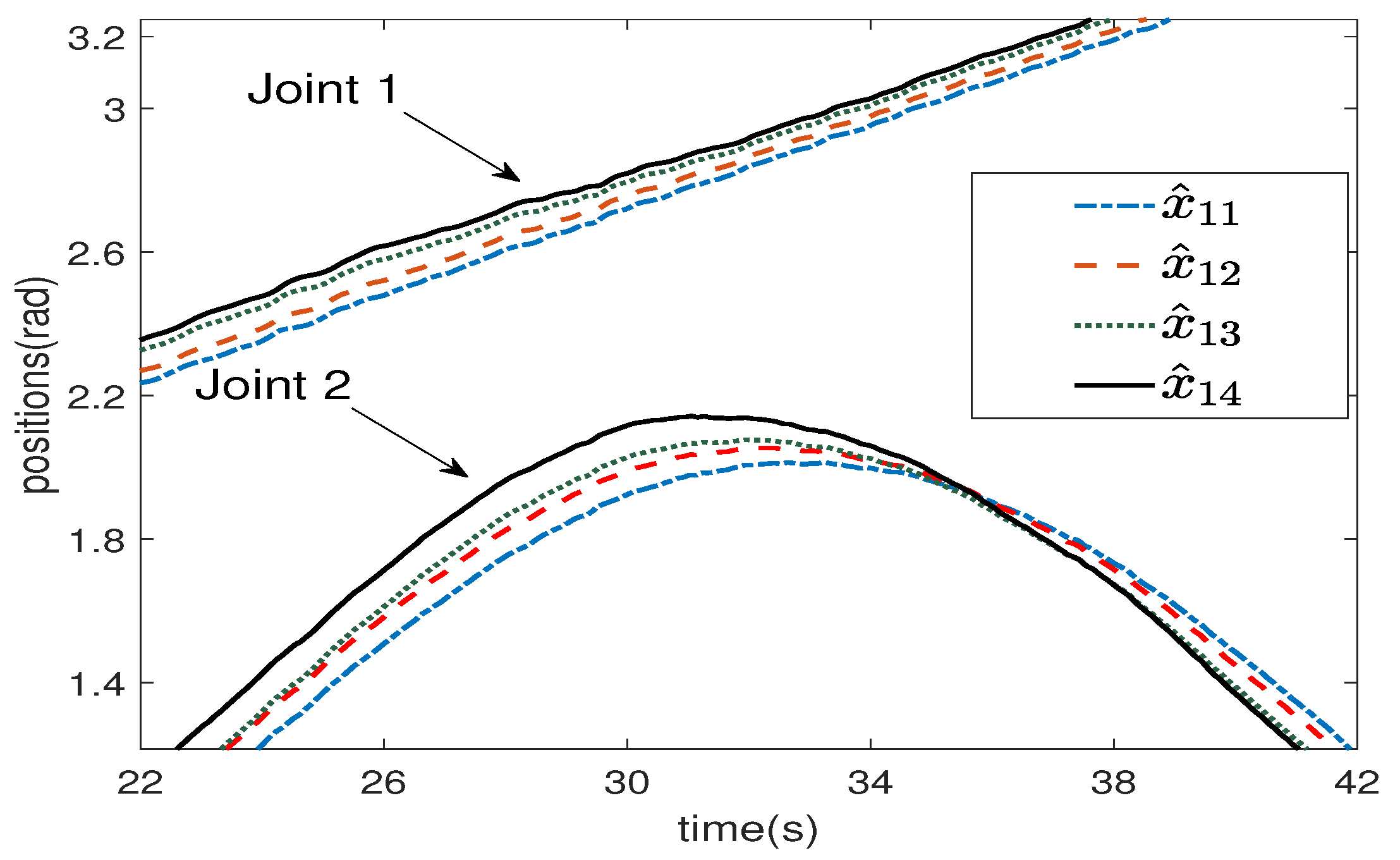
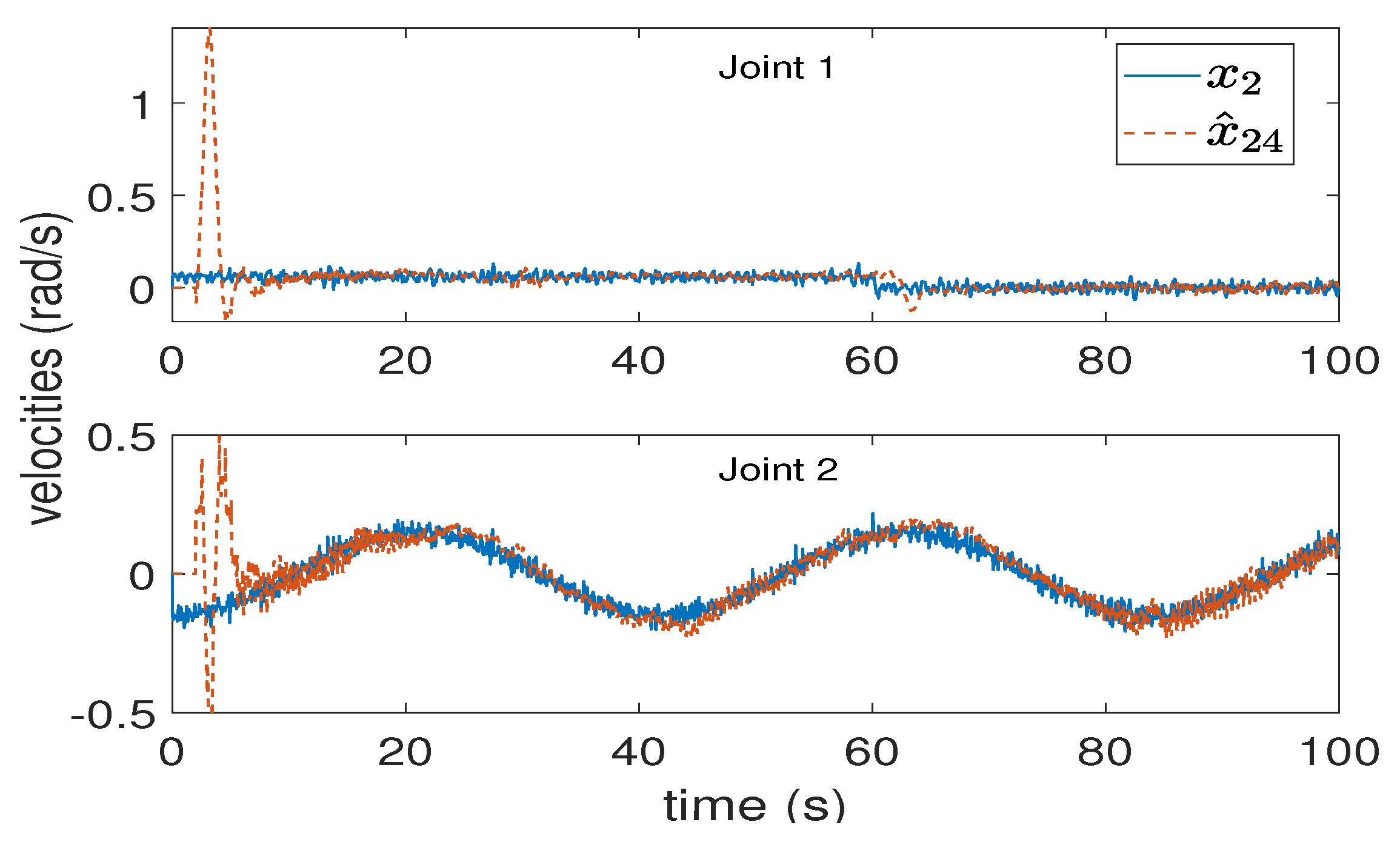
First, in the case that both delayed position and velocity measurements (i.e., y 1 ( t ) , y 2 ( t ) ) are available, the prediction results of joint positions and velocities are shown in Figure 1 and Figure 2, respectively, while the parameters of the predictors are set as m = 4 , k = 10 , α = 0.4 . It can be seen that both the predicted state x ^ 14 and x ^ 24 can coincide with the actual state x 1 and x 2 , while the measurements y 1 (the red dotted line in Figure 1) are conspicuously delayed. The effectiveness of proposed sequential predictor can be verified from these results. On the other hand, the predicted state variables x ^ 1 i of every sub-predictor ( i = 1 , 2 , 3 , 4 ) are given in Figure 3. As has been analyzed in Section 3, from Figure 3, each x ^ 1 i is a prediction of x ^ 1 , i 1 .
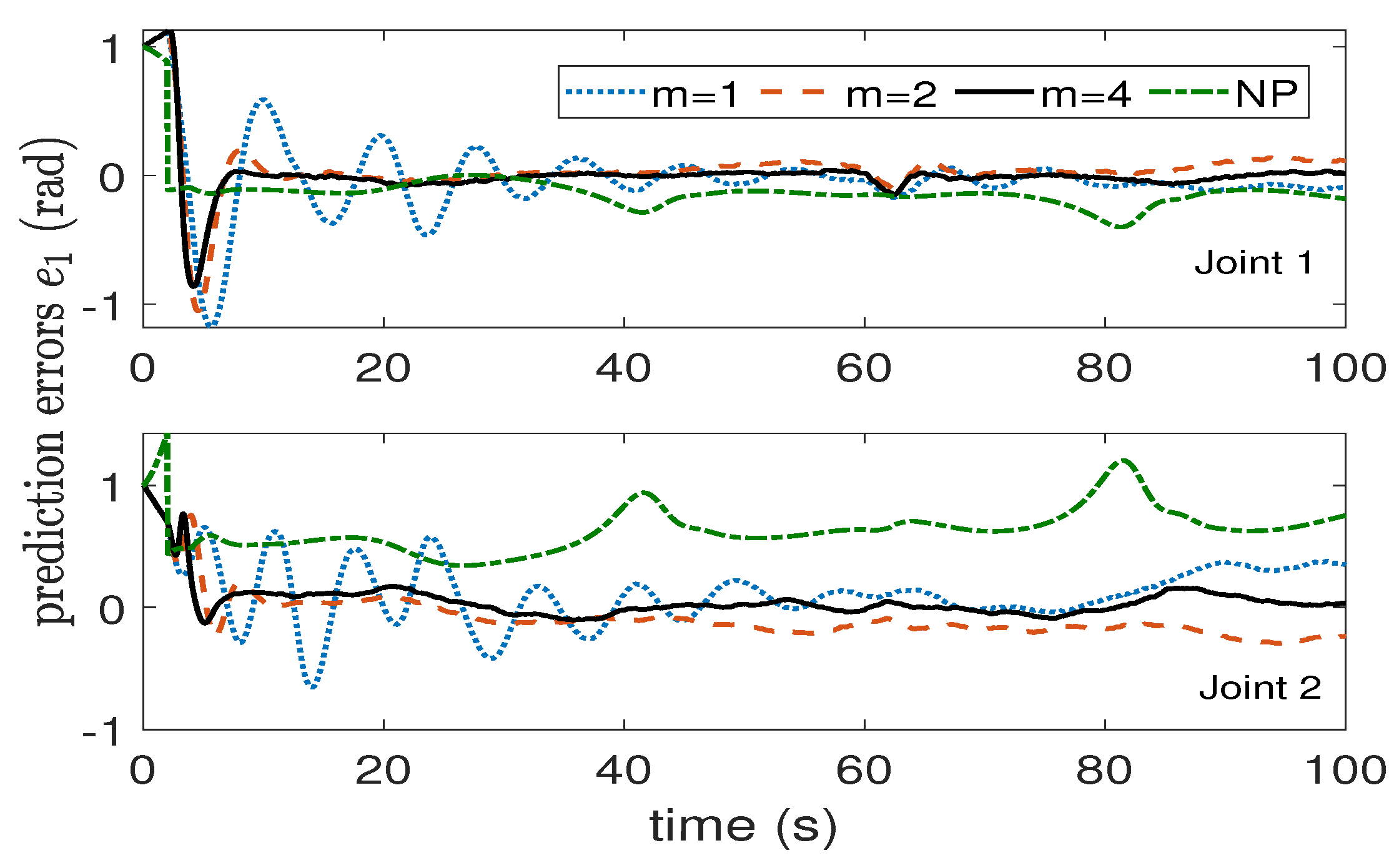
The prediction errors e 1 corresponding to different numbers of sub-predictors are compared in Figure 4, namely the parameters are designed as m = 1 , 2 , 4 , respectively, while k = 10 and α = 0.6 . The comparative results indicate that faster convergence of prediction errors can be obtained through using more sub-predictors. Moreover, the prediction error by utilizing the nonlinear predictor (NP) proposed in [19] has also been given in Figure 4. Because the NP is an open-loop predictor that is sensitive to the uncertainties and disturbances, it is clear in Figure 4 that a better performance with smaller prediction errors can be achieved from the proposed sequential predictor.
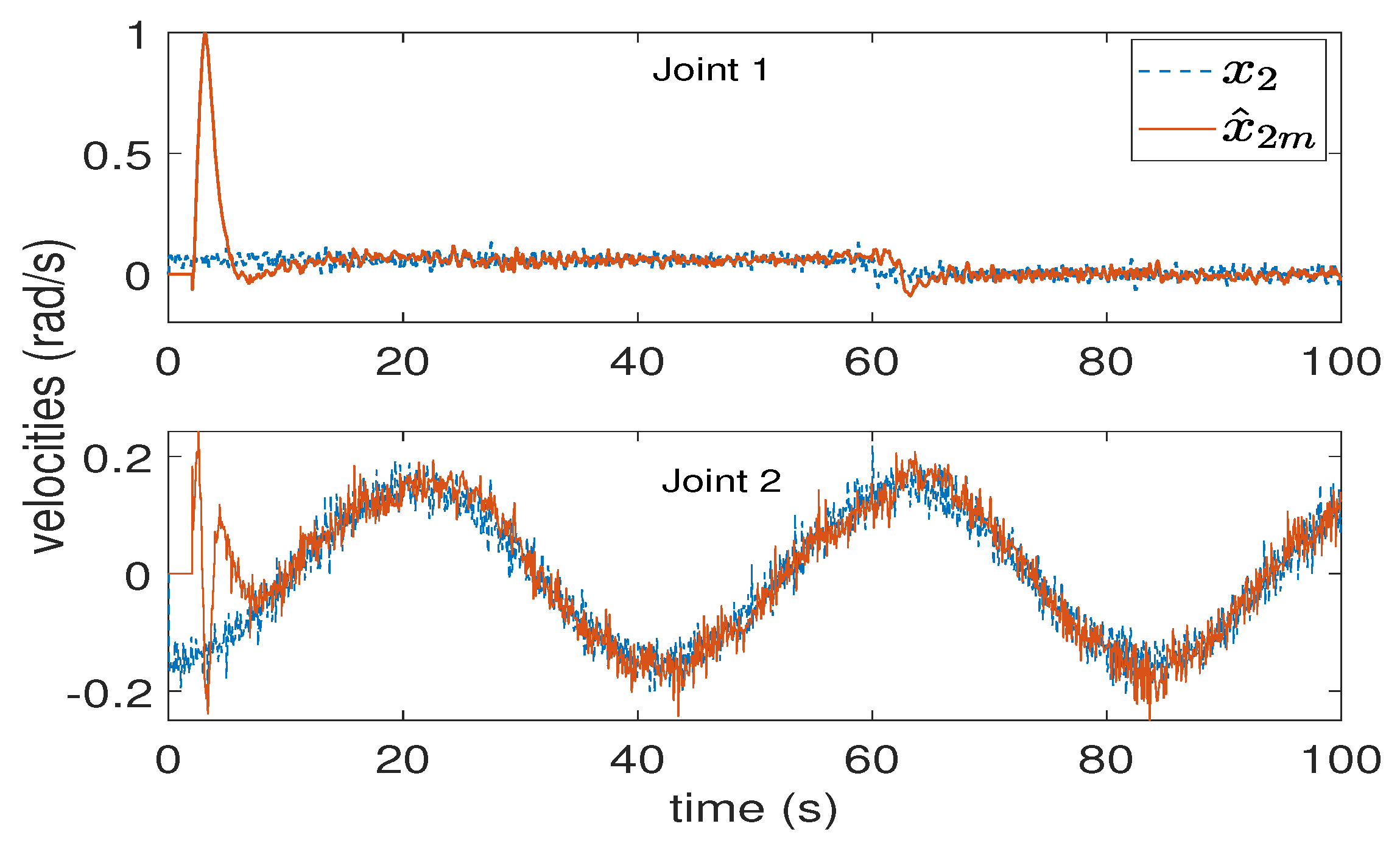
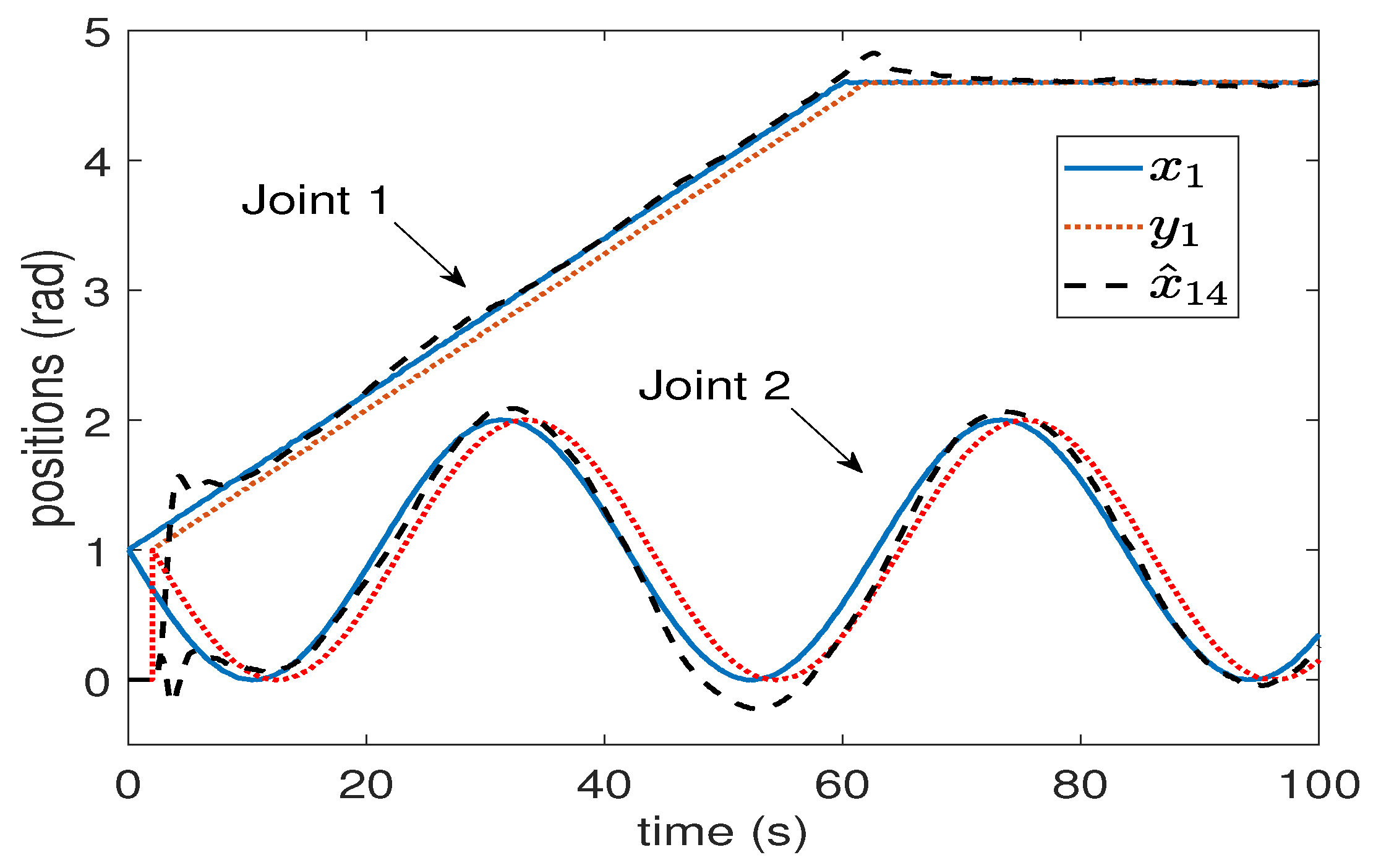
Second, in the case that only y 1 ( t ) is available, by applying Equation (44) to the predictor with parameters setting as γ = 5 , m = 4 , k = 10 , a = 0.5 , the prediction results of positions x 1 , x ^ 1 , y 1 ( t ) and velocities x 2 , x ^ 2 are given in Figure 5 and Figure 6, respectively. The results indicate that the predictions can converge to real ones, although the prediction errors, compared with Figure 1 and Figure 2, increased a bit due to the lacking velocity measurements. The effectiveness of proposed predictor without velocity measurements can be verified.
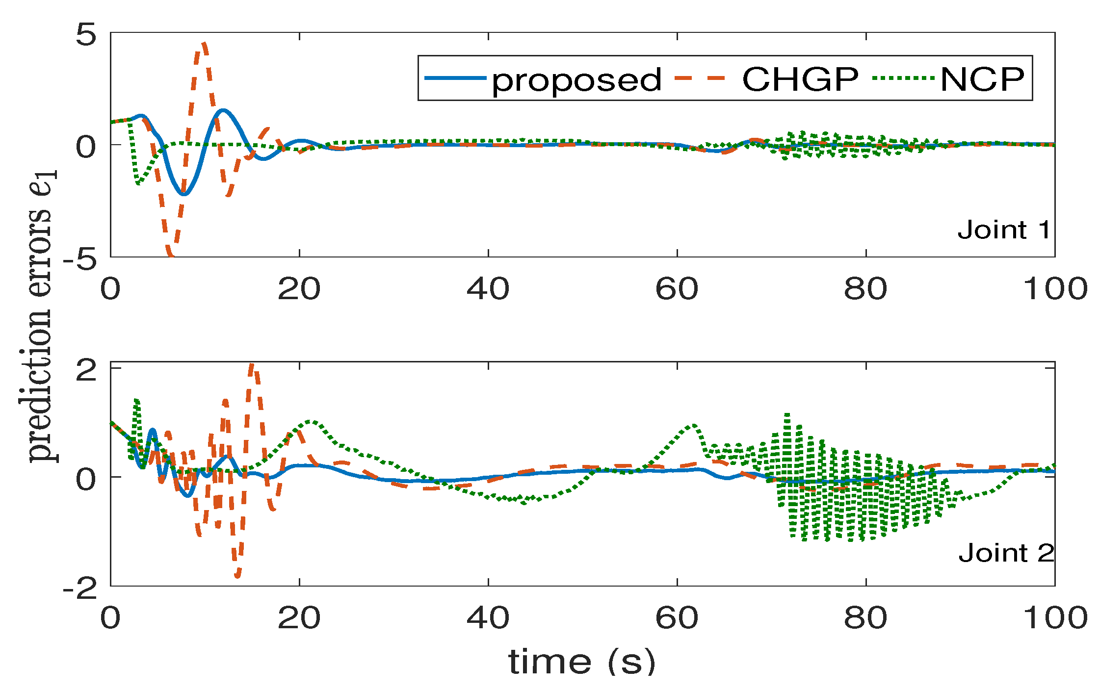
Finally, the proposed predictor is compared with the cascade high gain predictor (CHGP) [41] and nonlinear cascade predictor (NCP) [31] in the velocity-free case. In the performed simulations, the CHGP becomes unstable, with a large predictor gain when m = 4 . Thus, the parameters of three kinds of predictors are designed, same as m = 4 and k = 1 . The comparative results of the prediction errors are shown in Figure 7. Since the CHGP and CNP are designed based on Lipschitz nonlinearities, the prediction errors of these two predictors are larger than the proposed method. These results verify the stronger robustness to nonlinearities and large time delays of the proposed predictor in this paper.

6. Conclusions

In this paper, sequential predictors are proposed to estimate the actual states of uncertain Euler–Lagrange systems by using delayed outputs in the presence or absence of velocity signals. The large time delays are addressed with applying enough sub-predictors in a cascade structure. The parameter design method of the predictor is proposed to ensure the convergence of prediction errors based on Lyapunov method. Additionally, a simple modification approach of the first sub-predictor is presented to avoid the employment of velocity observers. From the simulation results, compared with other predictors, the good performance and robustness to nonlinearities and large time delays of the proposed predictor can be shown. Further, the output feedback control based on the proposed sequential predictor will be investigated, which could be applied to the robotic predictive control systems [8]. Another interesting direction is to develop event-triggered predictors [46] for systems with large communication delays.

Author Contributions

Conceptualization, S.S. and A.S.; methodology, S.S.; software, S.S. and L.F.; validation, S.S. and L.F.; formal analysis, T.L.; investigation, S.S. and T.L.; resources, A.S.; data curation, S.S.; writing—original draft preparation, S.S. and L.F.; writing—review and editing, A.S. and T.L.; visualization, S.S.; supervision, A.S.; project administration, A.S.; funding acquisition, A.S. All authors have read and agreed to the published version of the manuscript.

Funding

This work was supported in part by the Natural Science Foundation Program of Shandong Province under Grant no. ZR2022QF121.

Institutional Review Board Statement

Not applicable.

Informed Consent Statement

Not applicable.

Data Availability Statement

Not applicable.

Conflicts of Interest

The authors declare no conflict of interest. The funders had no role in the design of the study; in the collection, analyses, or interpretation of data; in the writing of the manuscript; or in the decision to publish the results.

References

  1. Makhbouche, A.; Boudjehem, B.; Birs, I.; Muresan, C. Fractional-order PID controller based on immune feedback mechanism for time-delay systems. Fractal Fract. 2023, 7, 53. [Google Scholar] [CrossRef]
  2. Li, X.; Li, P. Stability of time-delay systems with impulsive control involving stabilizing delays. Automatica 2021, 124, 109336. [Google Scholar] [CrossRef]
  3. Chen, Y.; Cao, Y.; Wang, R. Acoustic Source Tracking Based on Probabilistic Data Association and Distributed Cubature Kalman Filtering in Acoustic Sensor Networks. Sensors 2022, 22, 7160. [Google Scholar] [CrossRef] [PubMed]
  4. Zhao, K. Stability of a nonlinear Langevin system of ML-type fractional derivative affected by time-varying delays and differential feedback control. Fractal Fract. 2022, 6, 725. [Google Scholar] [CrossRef]
  5. Boonsatit, N.; Rajendran, S.; Lim, C.; Jirawattanapanit, A.; Mohandas, P. New adaptive finite-time cluster synchronization of neutral-type complex-valued coupled neural networks with mixed time delays. Fractal Fract. 2022, 6, 515. [Google Scholar] [CrossRef]
  6. Yang, X.; Liu, Y.; Cao, J.; Rutkowski, L. Synchronization of coupled time-delay neural networks with mode-dependent average dwell time switching. IEEE Trans. Neural Netw. Learn. Syst. 2020, 31, 5483–5496. [Google Scholar] [CrossRef]
  7. Chen, Y.; Zhang, G.; Wang, R.; Rong, H.; Yang, B. Acoustic vector sensor multi-source detection based on multimodal fusion. Sensors 2023, 23, 1301. [Google Scholar] [CrossRef]
  8. Yang, B.; Yan, G.; Wang, P.; Chan, C.; Song, X.; Chen, Y. A novel graph-based trajectory predictor with pseudo-oracle. IEEE Trans. Neural Netw. Learn. Syst. 2022, 33, 7064–7078. [Google Scholar] [CrossRef]
  9. Wang, Y.; Zhang, J.; Wu, H. Distributed adaptive mittag–leffler formation control for second-order fractional multi-agent systems via event-triggered control strategy. Fractal Fract. 2022, 6, 380. [Google Scholar] [CrossRef]
  10. Yan, B.; Lev-Ari, H.; Stanković, A.M. Networked state estimation with delayed and irregularly spaced time-stamped observations. IEEE Trans. Control Netw. Syst. 2017, 5, 888–900. [Google Scholar] [CrossRef]
  11. Hou, M.; Zítek, P.; Patton, R.J. An observer design for linear time-delay systems. IEEE Trans. Autom. Control 2002, 47, 121–125. [Google Scholar] [CrossRef]
  12. Sanz, R.; Garcia, P.; Fridman, E.; Albertos, P. Rejection of mismatched disturbances for systems with input delay via a predictive extended state observer. Int. J. Robust Nonlinear Control 2018, 28, 2457–2467. [Google Scholar] [CrossRef]
  13. Li, W.; Xie, Z.; Zhao, J.; Wong, P.K.; Wang, H.; Wang, X. Static-output-feedback based robust fuzzy wheelbase preview control for uncertain active suspensions with time delay and finite frequency constraint. IEEE/CAA J. Autom. Sin. 2020, 8, 664–678. [Google Scholar] [CrossRef]
  14. Wang, C.; Zuo, Z.; Lin, Z.; Ding, Z. A truncated prediction approach to consensus control of lipschitz nonlinear multiagent systems with input delay. IEEE Trans. Control Netw. Syst. 2016, 4, 716–724. [Google Scholar] [CrossRef]
  15. Astrom, K.J.; Hang, C.C.; Lim, B. A new smith predictor for controlling a process with an integrator and long dead-time. IEEE Trans. Autom. Control 1994, 39, 343–345. [Google Scholar] [CrossRef] [Green Version]
  16. Artstein, Z. Linear systems with delayed controls: A reduction. IEEE Trans. Autom. Control 1982, 27, 869–879. [Google Scholar] [CrossRef]
  17. Krstic, M. Input delay compensation for forward complete and strict-feedforward nonlinear systems. IEEE Trans. Autom. Control 2009, 55, 287–303. [Google Scholar] [CrossRef]
  18. Bekiaris-Liberis, N.; Krstic, M. Predictor-feedback stabilization of multi-input nonlinear systems. IEEE Trans. Autom. Control 2016, 62, 516–531. [Google Scholar] [CrossRef] [Green Version]
  19. Osuna-Ibarra, L.P.; Caballero-Barragan, H.; Loukianov, A. Predictor-based control for nonlinear mechanical systems with measurement delay. IFAC-PapersOnLine 2020, 53, 5783–5788. [Google Scholar] [CrossRef]
  20. Liberis, N.B.; Krstic, M. Stability of predictor-based feedback for nonlinear systems with distributed input delay. Automatica 2016, 70, 195–203. [Google Scholar] [CrossRef]
  21. Xu, X.; Liu, L.; Krstic, M.; Feng, G. Stability analysis and predictor feedback control for systems with unbounded delays. Automatica 2022, 135, 109958. [Google Scholar] [CrossRef]
  22. Mazenc, F.; Malisoff, M. Local stabilization of nonlinear systems through the reduction model approach. IEEE Trans. Autom. Control 2014, 59, 3033–3039. [Google Scholar] [CrossRef] [Green Version]
  23. Lei, J.; Khalil, H.K. High-gain-predictor-based output feedback control for time-delay nonlinear systems. Automatica 2016, 71, 324–333. [Google Scholar] [CrossRef] [Green Version]
  24. Cacace, F.; Germani, A.; Manes, C. An observer for a class of nonlinear systems with time varying observation delay. Syst. Control Lett. 2010, 59, 305–312. [Google Scholar] [CrossRef]
  25. Assche, V.V.; Ahmed-Ali, T.; Hann, C.; Lamnabhi-Lagarrigue, F. High gain observer design for nonlinear systems with time varying delayed measurements. IFAC Proc. Vol. 2011, 44, 692–696. [Google Scholar] [CrossRef] [Green Version]
  26. Sun, J.; Yang, J.; Zeng, Z. Predictor-based periodic event-triggered control for nonlinear uncertain systems with input delay. Automatica 2022, 136, 110055. [Google Scholar] [CrossRef]
  27. Sun, J.; Yang, J.; Li, S.; Zeng, Z. Predictor-based global sampled-data output feedback stabilization for nonlinear uncertain systems subject to delayed output. IEEE Trans. Autom. Control 2022, 68, 1839–1846. [Google Scholar] [CrossRef]
  28. Bhogaraju, I.; Farasat, M.; Malisoff, M.; Krstic, M. Sequential predictors for delay-compensating feedback stabilization of bilinear systems with uncertainties. Syst. Control Lett. 2021, 152, 104933. [Google Scholar] [CrossRef]
  29. Ahmed-Ali, T.; Cherrier, E.; Lamnabhi-Lagarrigue, F. Cascade high gain predictors for a class of nonlinear systems. IEEE Trans. Autom. Control 2011, 57, 221–226. [Google Scholar] [CrossRef] [Green Version]
  30. Germani, A.; Manes, C.; Pepe, P. A new approach to state observation of nonlinear systems with delayed output. IEEE Trans. Autom. Control 2002, 47, 96–101. [Google Scholar] [CrossRef]
  31. Farza, M.; Hernández-González, O.; Ménard, T.; Targui, B.; M’saad, M.; Astorga-Zaragoza, A.C.-M. Cascade observer design for a class of uncertain nonlinear systems with delayed outputs. Automatica 2018, 89, 125–134. [Google Scholar] [CrossRef]
  32. Farza, M.; M’Saad, M.; Menard, T.; Fall, M.L.; Gehan, O.; Pigeon, E. Simple cascade observer for a class of nonlinear systems with long output delays. IEEE Trans. Autom. Control 2015, 60, 3338–3343. [Google Scholar] [CrossRef]
  33. Battilotti, S. Continuous-time and sampled-data stabilizers for nonlinear systems with input and measurement delays. IEEE Trans. Autom. Control 2019, 65, 1568–1583. [Google Scholar] [CrossRef]
  34. Ramírez-Rasgado, F.; Farza, M.; M’Saad, M.; Hernández-González, O.; Astorga-Zaragoza, A.C. Observer design for a class of disturbed nonlinear systems with multirate sampled outputs involving multiple long time-varying delays. In Proceedings of the 2021 9th International Conference on Systems and Control (ICSC), Caen, France, 24–26 November 2021; pp. 493–498. [Google Scholar]
  35. Mazenc, F.; Malisoff, M.; Bhogaraju, I.N.S. Sequential predictors for delay compensation for discrete time systems with time-varying delays. Automatica 2020, 122, 109188. [Google Scholar] [CrossRef]
  36. Obuz, S.; Parikh, A.; Chakraborty, I.; Dixon, W. Lyapunov-based control of an uncertain euler-lagrange system with uncertain time-varying input delays without delay rate constraints. IFAC-PapersOnLine 2016, 49, 141–146. [Google Scholar] [CrossRef]
  37. Obuz, S.; Klotz, J.R.; Kamalapurkar, R.; Dixon, W. Unknown time-varying input delay compensation for uncertain nonlinear systems. Automatica 2017, 76, 222–229. [Google Scholar] [CrossRef]
  38. Kamalapurkar, R.; Fischer, N.; Obuz, S.; Dixon, W.E. Time-varying input and state delay compensation for uncertain nonlinear systems. IEEE Trans. Autom. Control 2015, 61, 834–839. [Google Scholar] [CrossRef] [Green Version]
  39. Yang, B.; Fan, F.; Ni, R.; Li, J.; Kiong, L.; Liu, X. Continual learning-based trajectory prediction with memory augmented networks. Knowl.-Based Syst. 2022, 258, 110022. [Google Scholar] [CrossRef]
  40. Shen, S.; Song, A.; Li, H.; Li, T. Cascade predictor for a class of mechanical systems under large uncertain measurement delays. Mech. Syst. Signal Process. 2022, 167, 108536. [Google Scholar] [CrossRef]
  41. Sajadi, M.; Ataei, M.; Ekramian, M. Cascade high-gain observers for a class of nonlinear systems with large delayed measurements. Int. J. Syst. Sci. 2018, 49, 2558–2570. [Google Scholar] [CrossRef]
  42. Tréangle, C.; Farza, M.; M’Saad, M. Observer design for a class of disturbed nonlinear systems with time-varying delayed outputs using mixed time-continuous and sampled measurements. Automatica 2019, 107, 231–240. [Google Scholar] [CrossRef]
  43. Sun, T.; Cheng, L.; Wang, W.; Pan, Y. Semiglobal exponential control of euler–lagrange systems using a sliding-mode disturbance observer. Automatica 2020, 112, 108677. [Google Scholar] [CrossRef]
  44. Sharma, N.; Bhasin, S.; Wang, Q.; Dixon, W.E. Predictor-based control for an uncertain euler–lagrange system with input delay. Automatica 2011, 47, 2332–2342. [Google Scholar] [CrossRef]
  45. Hua, C.; Liu, X. Delay-dependent stability criteria of teleoperation systems with asymmetric time-varying delays. IEEE Trans. Robot. 2010, 26, 925–932. [Google Scholar] [CrossRef]
  46. Yuan, J.; Chen, T. Switched fractional order multiagent systems containment control with event-triggered mechanism and input quantization. Fractal Fract. 2022, 6, 77. [Google Scholar] [CrossRef]
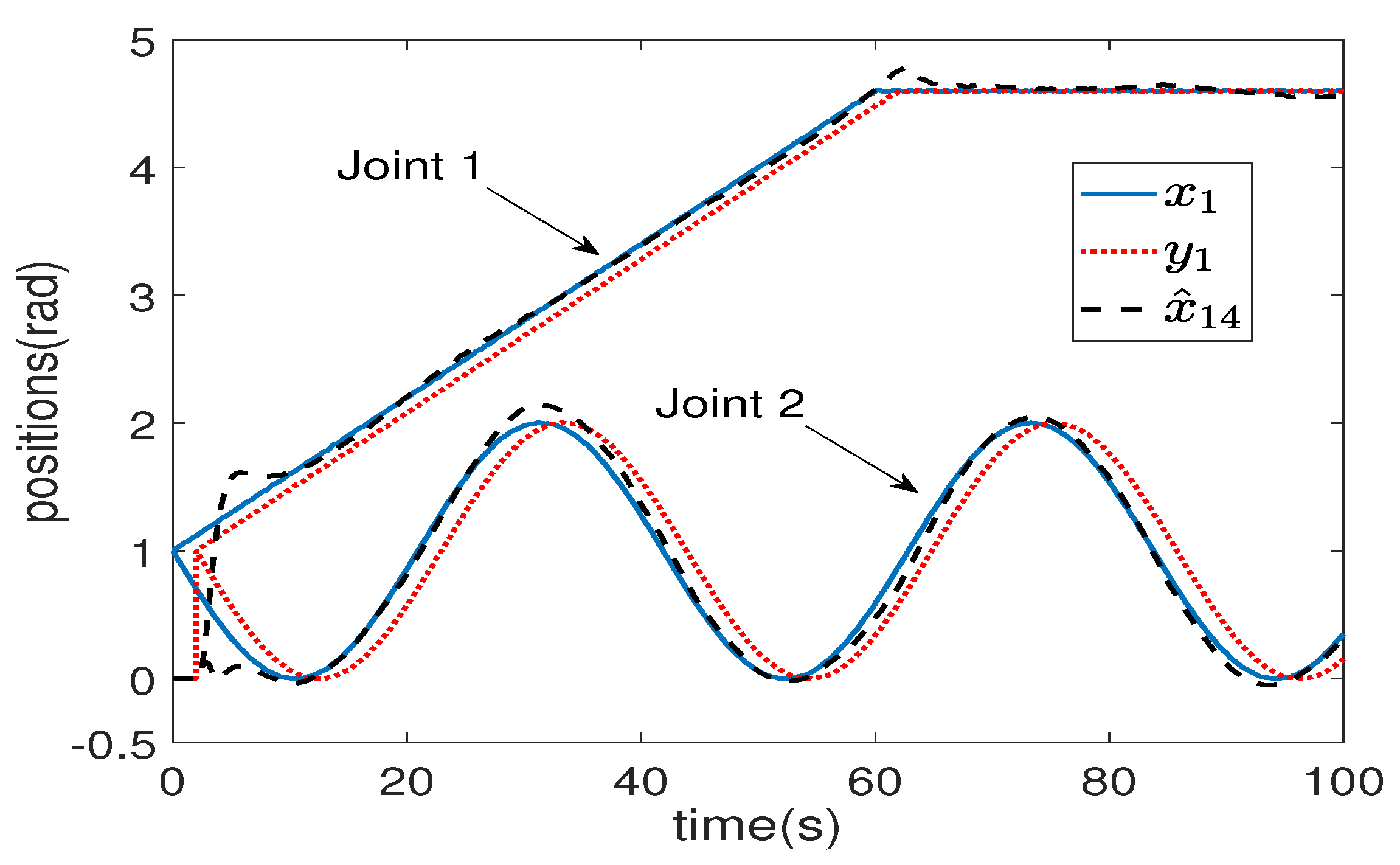
Figure 1. Prediction results of joint positions of a 2-DOF robot.
Fractalfract 07 00244 g001
Figure 2. Prediction results of joint velocities of a 2-DOF robot.
Fractalfract 07 00244 g002
Figure 3. Predicted states x ^ 1 i of every sub-predictors ( i = 1 , 2 , 3 , 4 ).
Fractalfract 07 00244 g003
Figure 4. Comparative results of e 1 with different m and NP.
Fractalfract 07 00244 g004
Figure 5. Prediction results of joint position without using velocity measurement.
Fractalfract 07 00244 g005
Figure 6. Prediction results of joint velocities without using velocity measurement.
Fractalfract 07 00244 g006
Figure 7. Comparative results of 3 kinds of predictors without using velocity measurements.
Fractalfract 07 00244 g007
Disclaimer/Publisher’s Note: The statements, opinions and data contained in all publications are solely those of the individual author(s) and contributor(s) and not of MDPI and/or the editor(s). MDPI and/or the editor(s) disclaim responsibility for any injury to people or property resulting from any ideas, methods, instructions or products referred to in the content.