Article

Neural Network-Based Adaptive Fractional-Order Backstepping Control of Uncertain Quadrotors with Unknown Input Delays

School of Engineering Technology, Purdue University, 401 Grant Street, West Lafayette, IN 47907, USA
*
Authors to whom correspondence should be addressed.
Fractal Fract. 2023, 7(3), 232; https://doi.org/10.3390/fractalfract7030232
Submission received: 31 January 2023 / Revised: 27 February 2023 / Accepted: 4 March 2023 / Published: 5 March 2023

Abstract

:
Adaptive control is essential and effective for reliable quadrotor operations in the presence of uncertain modeling parameters and unknown time-delayed inputs. This paper presents an original radial basis function neural network-based adaptive fractional-order backstepping controller (RBF-ADFOBC). The nonlinearity of the time-delayed inputs is eliminated by introducing an augmented state variable via Pade’s approximation method. For each subsystem in the quadrotor dynamics, a companioned second-order compensation system is developed. The candidate Lyapunov functions are then properly designed by incorporating the control errors, parameter uncertainties and estimation errors of the neural networks’ weight vectors. It is shown that the semi-globally uniformly ultimately boundedness of all the state variables and the estimation error of uncertain parameters can be guaranteed. In addition, the trajectory-tracking error of the state variables can be driven to an adjustable small neighborhood of origin by properly setting the selectable parameters. Numerical simulations reveal that the tracking performance of the proposed controller can be improved continuously as the fractional order increases to a specific positive value, and the controller with a negative order may demonstrate higher robustness to the modeling uncertainties. Favorably, the comparison to the other two previous controllers further reveals the superior tracking accuracy and robustness of the proposed RBF-ADFOBC controller.

1. Introduction

A quadrotor is a type of helicopter with its lifting force generated via the rotations of four rotors [1,2]. Quadrotors have been witnessed in a large number of applications such as disaster rescue, forest fire surveillance, battlefield air control and topographical mapping [3,4]. Due to the high demand for reliable autonomous navigation of quadrotors in complex environments, e.g., the transportation of heavy loads through confined pipelines, effective control schemes with high path tracking accuracy and robustness to modeling uncertainties are necessary for quadrotors [5,6]. In addition, importantly, the time delays arising from the computational latency of sensors, actuators and edge computing units in the quadrotors bring new challenges for controller design [7,8].
In view of the underactuated, strongly coupled characteristics of quadrotors, multiple types of controllers have been developed, including the proportional integral derivative (PID) control [9], the sliding mode control [10], the backstepping control [11], the neural network control [11], the adaptive control [11], etc. However, due to external disturbances and time delays in control signals, these controllers may exhibit certain limitations. For instance, the conventional PID controller usually leads to large system overshoot and hardly adapts the system to external disturbances. Some traditional nonlinear control strategies, such as sliding mode control and backstepping control, guarantee the global stability of the quadrotor system by introducing Lyapunov functions, but these approaches alone cannot mitigate the effects of external disturbances and input time delays either. Neural network control, on the other hand, utilized the neural networks to learn the full picture of a quadrotor system, including the unmodeled dynamics, thus it provides an effective strategy for handling intractable system characteristics (e.g., nonlinearity, unboundedness) [12]. In contrast, the conventional adaptive controllers can compensate for the changes of uncertain parameters in real time, but the development of the adaptive control laws needs to consider the dynamics of the system itself, and some unwieldy feedback variables may cause the instantaneous expansion of the control rates and even the sudden collapse of the whole system [11]. To cope with the limitations of the aforementioned controllers, researchers have tried to combine two or more control strategies to complement each other and form new controllers with high overall control performance and improved robustness [13,14]. Notable examples for quadrotors include adaptive control via sliding mode and neural networks [15]. A hybrid control algorithm that combined the advantages of a PID approach with a multi-loop approach was proposed, delivering greatly improved performance in quadcopter altitude control [16]. Through an extended state observer, a robust backstepping trajectory-tracking controller for the quadrotor under control input saturation was proposed, which advances the current state of the art in three ways: it does not require full state information, it can account for the presence of lumped disturbances, and it was verified as being stable using Lyapunov theory [17]. More attractively, a nonlinear control method, by combining the adaptive sliding mode controller with an unknown time-varying parameter and a water discharge system, was proposed. The method delivers a significantly improved performance with regard to both settling time and robustness against the varying terms [18]. An adaptive radial basis function neural network-based active disturbance rejection controller (RBF-ADRC) was developed, and the authors proved that the anti-disturbance, robustness and tracking accuracy of the RBF-ADRC are better than the traditional ADRC and PID control methods [19]. Similarly, a quadrotor system based on a backpropagation neural network and adaptive linear active disturbance rejection control (ALADRC) was then demonstrated [20]. A common feature of these controllers discussed so far is that their derivation depends completely on the nonlinear transformation of the integer-order system state variables or the integer-order gradient-based optimization of the energy functions. Additionally, this feature in some sense may hinder the exploration of controllers with better performance.
Over the last few decades, the introduction of fractional calculus theory into automatic control has led to the emergence of new ideas and potentially more effective control schemes [21,22,23,24,25,26,27,28,29,30]. Compared to conventional integer-order controllers, there are at least two strengths of fractional-order controllers [31,32]. Firstly, the fractional-order state variables act as the intermediate interpolation of two consecutive integer-order states. As nonlocal operators, fractional-order integration and differentiation make fuller use of the memory information of the state variables, and thus, exhibit stronger time sensitivity than integer-order operators [33]. This suggests that as the state spectrum of the system expands toward fractional orders, the controller may achieve stronger suppression of the time-sensitive error components. In addition, the fractionalization of control laws will bring additional adjustable parameters, which may compensate for the errors brought by unmodeled system dynamics. Recently, a growing number of successful fractional-order control trials has been witnessed, such as a fuzzy fractional-order PD vibration control of uncertain building structures [34], a linear matrix inequality optimization-based H control of switched delay systems with linear fractional perturbations [35], a combined backstepping and fractional-order PID controller for trajectory tracking of mobile robots [36], an SA-PSO optimized fractional PID (FOPID) control of quadrotors [37], a fractional-order sliding mode control of quadrotors [38] and an adaptive fractional-order PID control of a quadrotor [39]. These enlightening examples motivate us to develop a fractional-order adaptive backstepping and neural networks control strategy.
The control of quadrotor systems poses several difficulties due to their highly nonlinear, time-varying and uncertain dynamics. In particular, nonlinear time-delayed inputs, modeling uncertainties and unmodeled dynamics are significant challenges that must be addressed for effective control. In this work, we propose a novel RBF neural network-based adaptive fractional-order backstepping controller (RBF-ADFOBC) for quadrotor systems that can overcome these difficulties. Our approach uses Pade’s approximation to convert the nonlinear time-delayed inputs into a linear combination of an augmented state variable and system state variable, and incorporates second-order compensation and RBF neural networks to approximate the intractable parts of the augmented state-space model. Moreover, the Lyapunov function candidates are designed to incorporate the modeling uncertainties and neural network approximation errors, and a fractional-order integral (derivative) term is added to the virtual control laws, resulting in generalized fractional-order control laws. Our approach also includes online adaptation of the RBF neural networks and the uncertain parameters to compensate for the unmodeled dynamics and time delays in the inputs, resulting in a more robust and adaptive control system. The proposed RBF-ADFOBC can guarantee that all the signals in the closed-loop system are semi-globally uniformly ultimately bounded (SGUUB) and can be applied not only to any type of quadrotor with different geometrical parameters, but can also be extended to the control of other high-order, nonlinear, strongly coupled and uncertain systems. The feasibility of the RBF-ADFOBC is demonstrated through numerical simulations, including comparison to the SA-PSO optimized FOPID controller [37] and a linear quadratic regulator (LQR) controller with an integrative action term [40]. Overall, our work contributes a new and effective approach to the control of quadrotor systems and addresses several significant difficulties, while improving the performance and robustness of the control system.

2. Preliminaries

The fractional integral and Caputo’s fractional derivative are given in this section and will be used later. The α -th order Caputo’s fractional derivative of a function f ( t ) is [22]:
D t 0 C t β f ( t ) = 1 Γ ( n β ) t 0 t f ( n ) ( τ ) ( t τ ) β n + 1 d τ
where n 1 < β < n + and Γ ( x ) = 0 e τ τ x 1 d τ for x is the gamma function. The fractional integral of an integrable function f ( t ) is defined by [22]:
I t 0   t β f ( t ) = 1 Γ ( β ) t 0 t f ( τ ) ( t τ ) 1 β d τ
where β + is the order of the fractional integral. Then, in this work, D β is taken as the unified notation for Caputo’s fractional derivative and fractional integral, where D β = D t 0 C t β for β > 0 and D β = I t 0   t β for β < 0 . The properties of D β are summarized as follows:
Property 1 (Linear property [25]): Fractional derivative (integral) operator is linear, i.e., given functions f ( t ) and g ( t ) ,
D β [ a f ( t ) + b g ( t ) ] = a D β f ( t ) + b D β g ( t )
holds for any constants a and b .
Property 2 (Interpolation property [25]): Fractional derivative (integral) operator is the interpolation of the integer-order derivative (integral) operators, i.e.,
lim β n D β f ( t ) = f ( n ) ( t ) lim β n 1 D β f ( t ) = f ( n 1 ) ( t )
holds for n 1 < β < n .
Property 3 (Composition with integer derivatives [25]): Fractional derivative (integral) operator composes with integer-order derivative by
D β ( d m d t m f ( t ) ) = ( 1 ) D β + m f ( t ) = ( 2 ) d m d t m ( D β f ( t ) )
where the equality (1) is deduced from the definition of Caputo’s fractional derivative and the equality (2) holds for f ( s ) ( 0 ) = 0 , s = n , n + 1 , , m ( m = 0 , 1 , ; n 1 < β < n ).
In real implementations, the fractional derivative (integral) operations can be tackled in s space via the Laplace transform. The Laplace transform of D β f ( t ) is given by [25]:
{ D β f ( t ) } = { s β F ( s ) ,         if   β 0 s β F ( s ) k = 0 n 1 s β k 1 f ( k ) ( 0 ) ,         if   β > 0
where F ( s ) is the Laplace transform of f ( t ) . The fractional-order operators can be estimated using the Oustaloup filter [41], i.e.,
s β K n = 1 N s z n s p n
where z n and p n ( n = 1 , 2 , , N ) are zeros and poles, K is a gain factor, and N is the order of the Oustaloup filter. In the Oustaloup filter, 0 < β < 1 can be assumed since s β = s | β | s β | β | if β | β | , where | β | is the floor integer part of β . In addition to the basics of fractional calculus, the following definition for the radial basis function neural network (RBF NN) is needed for the controller design. The RBF NN employs linearly weighted RBF kernels to approximate the unknown function F ( x ) :   n , i.e., [42]
F ( x ) = w T S ( x ) + δ ( x )
where x Ω x n is the input vector and the training inputs are selected from a compact subset Ω x . w = [ w 1 , w 2 , , w l ] T l is the weight vector and l is the number of basis neurons in the RBF NN. δ ( x ) is the estimate error. S ( x ) = [ s 1 ( x ) , s 2 ( x ) , , s l ( x ) ] T l ( Ω x ) is the basis function vector, and s i ( x ) is given as:
s i ( x ) = exp [ ( x μ i ) T ( x μ i ) / η i 2 ]
where μ i = [ μ i 1 , μ i 2 , , μ i n ] T is the center of the receptive field and η i denotes the standard deviation of the Gaussian. Note that in practice there should be an error for this approximation, and the ideal weight vector is defined by:
W = arg min w l { sup x Ω x | F ( x ) w T S ( x ) | }

3. Dynamic Model of Quadrotor UAV

The dynamic model developed in this work follows the notations shown in Figure 1, where the subscripts b and e denote the body and the earth coordinate systems, respectively. The rotational motion (i.e., roll angle ϕ , pitch angle θ and yaw angle ψ ) in the attitude subsystem is described in the body frame, and the translational motion (i.e., linear positions x , y and z of the mass center) is described in the earth frame. To derive the dynamic model of the quadrotor UAV, several assumptions need to be made: the thrust and drag of each rotor are considered to be proportional to the squared angular velocity of the propeller. The quadrotor flies at low speed indoors or outdoors without wind, so air resistance is negligible. Due to a high degree of symmetry in the rigid structure, the inertia matrix of the quadrotor is symmetric with the trial nondiagonal components. In addition, the moment of inertia J r can be omitted given the small mass and volume of the rotors. Based on these assumptions, the translational and rotational dynamics of the uncertain quadrotor can be given in Equation (11):
x ¨ = sin θ cos ϕ cos ψ + sin ϕ sin ψ u 1 t τ 1 m + d 1 y ¨ = sin θ cos ϕ sin ψ sin ϕ cos ψ u 1 t τ 1 m + d 2 z ¨ = cos θ cos ϕ u 1 t τ 1 m g + d 3 ϕ ¨ = I y I z θ ˙ ψ ˙ + u 2 t τ 2 I x + d 4 θ ¨ = I z I x ϕ ˙ ψ ˙ + u 3 t τ 3 I y + d 5 ψ ¨ = I x I y ϕ ˙ θ ˙ + u 4 t τ 4 I z + d 6
where x , y and z are translational coordinates in the earth frame system, and ϕ , θ and ψ are the roll angle, pitch angle and yaw angle, respectively, in the body frame system. where m is the mass of the quadrotor, and I x , I y and I z are the three diagonal components of the inertia matrix. where d i   ( i = 1 , 2 , , 6 ) are the unknown external disturbances on the position and attitude subsystems, and τ 1 , τ 2 , τ 3 and τ 4 are the time delays of the virtual control inputs. Moreover, u 1 , u 2 , u 3 and u 4 are the time-delayed control inputs, which are related to the rotational speed of the four rotor motors by:
{ u 1 = b ( Ω 1 2 + Ω 2 2 + Ω 3 2 + Ω 4 2 ) u 2 = l b ( Ω 4 2 Ω 2 2 ) u 3 = l b ( Ω 3 2 Ω 1 2 ) u 4 = d ( Ω 1 2 + Ω 2 2 Ω 3 2 + Ω 4 2 )
where b is the is the lift coefficient, d is the drag coefficient, and l is the distance between the center of mass of the UAV and the four rotor axes. where Ω 1 , Ω 2 , Ω 3 and Ω 4 are the angular velocities of the four rotors, respectively. In this work, the nominal values for the model parameters of an uncertain quadrotor UAV system are presented in Table 1, and these nominal values are obtained from measurements and the manufacturer’s specifications. It should be mentioned that the adaptive control laws will be proposed in terms of the virtual controls (i.e., u 1 , u 2 , u 3 and u 4 ). In this sense, the uncertainty in the aerodynamics and geometry-related model parameters (e.g., b , l and d in Equation (2)) will not be considered in this work. In addition, for the clarity and unification of notations, the state variables in the state-space model are specified as x 1 = x , x 2 = x ˙ , x 3 = y , x 4 = y ˙ , x 5 = z , x 6 = z ˙ , x 7 = ϕ , x 8 = ϕ ˙ , x 9 = θ , x 10 = θ ˙ , x 11 = ψ and x 12 = ψ ˙ . Besides, two assumptions are required in this work:
Assumption (1): The uncertain external disturbances, d i   ( i = 1 , 2 , , 6 ) in Equation (11), are bounded by known upper bounds, denoted by D i   ( i = 1 , 2 , , 6 ) .
Assumption (2): The desired trajectory x i d of the state variables are second-order continuous, i.e., x i d C 2 ( [ 0 , ) ) for i = 1 , 3 , 5 , 7 , 9 , 11 . Thus, x i d , x ˙ i d and x ¨ i d are bounded.
Figure 1. The schematic of the quadrotor UAV system.
Fractalfract 07 00232 g001
Table 1. Nominal values for the parameters of an uncertain quadrotor UAV.
ParameterNominal ValueParameterNominal Value
m 0.53 kg I x 6.228 × 10 3 kg·m2
I y 6.228 × 10 3 kg·m2 I z 1.121 × 10 2 kg·m2
l 0.232 m b 3.130 × 10 5
d 7.500 × 10 7 g 9.8 m/s2

4. Controller Design

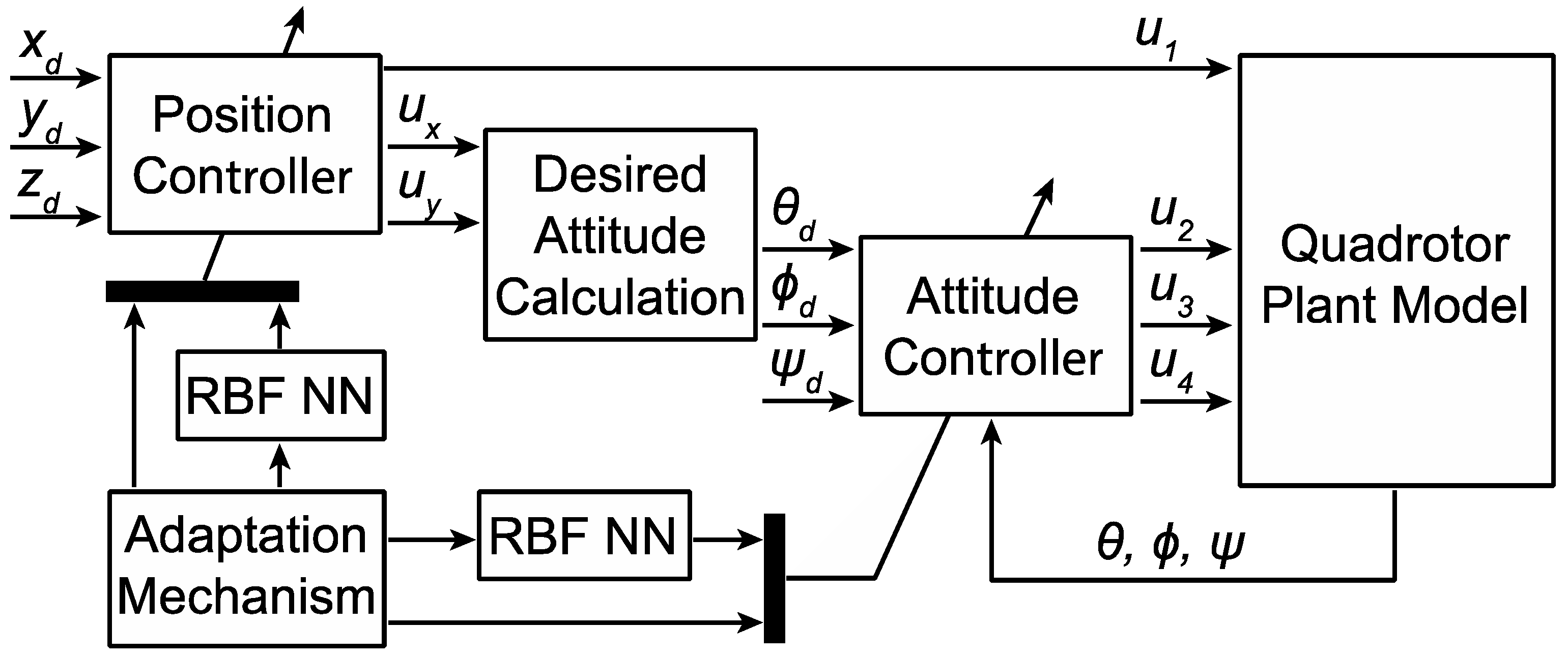
As shown in Figure 2, to cope with the semi-coupling relationship between the position and attitude subsystems, the inner loop (attitude control) is designed first, and the outer loop (position control) follows. The inner control loop aims to ensure the stability of the quadrotor when it is steadily flying or staying in a fixed position. The outer loop is to achieve the tracking control of the quadrotor to the target path. In Figure 2, x d , y d , z d are the desired tracking position of the quadrotor, and θ d , ϕ d and ψ d are the desired attitude angle to be tracked. Define the virtual control inputs for the position subsystem as:
{ u x = ( sin θ cos ϕ cos ψ + sin ϕ sin ψ ) u 1 ( t τ 1 ) u y = ( sin θ cos ϕ sin ψ sin ϕ cos ψ ) u 1 ( t τ 1 ) u z = ( cos θ cos ϕ ) u 1 ( t τ 1 )
Substitute Equation (13) into Equation (11), the position subsystem can be reformulated as:
{ x ¨ = 1 m u x ( t τ 1 ) + d 1 y ¨ = 1 m u y ( t τ 1 ) + d 2 z ¨ = 1 m u z ( t τ 1 ) g + d 3
The outer loop (position) controller achieves the adaptive tracking control of the position subsystem in Equation (14) using three virtual controls: u x , u y and u z . Then, given the desired yaw angle ψ d , inverting Equation (13) yields the desired roll and pitch angles that can be used by the inner loop (attitude) controller:
{ u 1 = u z cos θ cos ϕ ϕ d = arcsin ( u x sin ψ d u y cos ψ d u 1 ) θ d = arcsin ( u x u 1 sin ϕ sin ψ d cos ϕ cos ψ d )
Figure 2. Schematic diagram of the closed-loop neural network-based adaptive quadrotor control system.
Fractalfract 07 00232 g002

4.1. Position Control

As indicated in Equation (14), the virtual controls u x , u y and u z in the position subsystem have the same unknown time delays, τ 1 . To resolve the unknown input delays in the virtual controls, Pade’s approximation approach is used in this work. Pade’s approximation is a volatile transformation approach to approximate the nonlinear function with linear functionals. For instance, with the Laplace transform of u x ( t τ 1 ) , one has:
  { u x ( t τ 1 ) } = exp ( τ 1 s ) { u x ( t ) } = exp ( τ 1 s / 2 ) exp ( τ 1 s / 2 ) { u x ( t ) } 1 τ 1 s / 2 1 + τ 1 s / 2 { u x ( t ) }
For further investigation, an additional variable y 2 is introduced to make the following equation hold,
1 τ 1 s / 2 1 + τ 1 s / 2 { u x ( t ) } = { y 2 } { u x ( t ) }
Then, it is straightforward to find that ux(tτ1) ≈ y2ux(t) and an additional differential equation can be deduced from Equation (17), i.e.,
y ˙ 2 = 2 τ 1 y 2 + 4 τ 1 u x ( t )
In the position subsystem, if x1 = x and x 2   =   x ˙ , the second-order differential equation in the x direction can be represented as:
{ x ˙ 1 = x 2 x ˙ 2 = 1 m y 2 1 m u x ( t ) + d 1 y ˙ 2 = 2 τ 1 y 2 + 4 τ 1 u x ( t )
where Equation (19) can be treated as an augmented state-space model of the position subsystem in the x direction.
Remark 1: Inspect Equation (19) and follow the standard backstepping derivations, it will find that the estimate error associated with y 2 , i.e., y ˜ 2 = y 2 y ^ 2 , with y ^ 2 being the estimate of y 2 , cannot be eliminated in the final step. This problem arises from the virtual control u x ( t ) that is present in two separate equations of the augmented state-space model. Unfortunately, this issue has not been fully resolved in previous literature, e.g., [43,44,45,46]. In this work, a compensation state-space system is proposed to tackle this issue and it will show that all the estimate errors of the augmented state-space model in Equation (19) are eliminated with the aid of the compensation system in Equation (20),
{ y ˙ 1 = τ 1 2 m y 2 λ 1 τ 1 2 y 1 y ˙ 2 = 2 τ 1 y 2 + 4 τ 1 u x ( t )
where λ 1 > 0 is a selectable positive parameter. Before the controller design, the following change of coordinates are introduced:
{ z 1 = x 1 x 1 d y 1 z 2 = x 2 α 1 x ˙ 1 d + τ 1 2 m y 2
where x 1 d is the desired trajectory of the state variable x 1 (i.e., x ) in the position subsystem and α 1 is a virtual control to be designed. The adaptive fractional-order backstepping controller for the position subsystem in the x direction is derived as follows:
Step 1: Consider the following candidate Lyapunov function,
V 1 = 1 2 z 1 2 + 1 2 γ 11 θ ˜ 11 2
where γ 11 > 0 is a selectable positive parameter, θ ˜ 11 = θ 11 θ ^ 11 is the estimate error of the unknown model parameter, θ 11 . Here, θ ^ 11 is an estimate of θ 11 , and θ 11 will be defined later. Given Equations (19)–(21), the first derivative of V 1 can be given as:
V ˙ 1 = z 1 ( x 2 x ˙ 1 d + τ 1 2 m y 2 + λ 1 τ 1 2 y 1 ) 1 γ 11 θ ˜ 11 θ ^ ˙ 11 = z 1 ( z 2 + α 1 + λ 1 τ 1 2 y 1 ) 1 γ 11 θ ˜ 11 θ ^ ˙ 11
From Young’s inequality, one has:
z 1 z 2 z 1 2 2 + z 2 2 2 z 1 2 + z 2 2 2
Substituting Equation (24) into Equation (23) yields:
V ˙ 1 z 1 ( z 1 + α 1 + λ 1 τ 1 2 y 1 ) + 1 2 z 2 2 1 γ 11 θ ˜ 11 θ ^ ˙ 11 = z 1 ( z 1 + α 1 + F 1 ( y 1 ) ) + 1 2 z 2 2 1 γ 11 θ ˜ 11 θ ^ ˙ 11
where F 1 ( y 1 ) = λ 1 τ 1 y 1 / 2 is an intractable function, whose boundedness is unknown. Thus, RBF NN is utilized to approximate this intractable function,
V ˙ 1 z 1 ( z 1 + α 1 + W 1 T S 1 ( y 1 ) + δ 1 ( y 1 ) ) + 1 2 z 2 2 1 γ 11 θ ˜ 11 θ ^ ˙ 11 z 1 ( z 1 + α 1 + z 1 2 a 1 | | W 1 | | 2 S 1 T S 1 ) + a 1 W 1 T W 1 2 | | W 1 | | 2 + z 1 2 2 + ϵ 1 2 2 + z 2 2 2 1 γ 11 θ ˜ 11 θ ^ ˙ 11 = z 1 ( 3 2 z 1 + α 1 + b 1 z 1 2 a 1 θ 11 S 1 T S 1 ) + a 1 2 + ϵ 1 2 2 + z 2 2 2 1 γ 11 θ ˜ 11 θ ^ ˙ 11
where a 1 > 0 and b 1 > 0 are two selectable positive parameters, the unknown parameter θ 11 = | | W 1 | | 2 / b 1 , which inherits the uncertainty of the ideal weight vector, W 1 . where ϵ 1 denotes an error bound of the RBF NN approximation. Then, the virtual control and the adaptive laws can be set as:
α 1 = ( c 11 + 3 2 ) z 1 b 1 z 1 2 a 1 θ ^ 11 S 1 T S 1 h 1 ( D β 1 z 1 z 1 ) e r 1 t
θ ^ ˙ 11 = γ 11 b 1 z 1 2 2 a 1 S 1 T S 1 ν 11 θ ^ 11
where c 11 > 0 , h 1 > 0 , ν 11 > 0 and r 1 > 0 are four selectable positive parameters and D β 1 is the fractional derivative operator with order 1 < β 1 < 1 . Substituting Equations (27) and (28) into Equation (26), one has:
V ˙ 1 c 11 z 11 2 + a 1 2 + ϵ 1 2 2 + z 2 2 2 + ν 11 γ 11 θ ˜ 11 θ ^ 11 h 1 z 1 ( D β 1 z 1 z 1 ) e r 1 t
Since Young’s inequality gives θ ˜ 11 θ ^ 11 = θ ˜ 11 ( θ 11 θ ˜ 11 ) θ 11 2 / 2 θ ˜ 11 2 / 2 , one has:
V ˙ 1 c 11 z 11 2 ν 11 2 γ 11 θ ˜ 11 2 + a 1 2 + ϵ 1 2 2 + z 2 2 2 + ν 11 2 γ 11 θ 11 2 h 1 z 1 ( D β 1 z 1 z 1 ) e r 1 t
Step 2: Consider the following Lyapunov function,
V 2 = V 1 + 1 2 z 2 2 + θ ˜ 12 2 2 γ 12 θ 12 + θ ˜ 13 2 2 γ 13
where γ 12 > 0 and γ 13 > 0 are two selectable positive parameters, θ ˜ 12 = θ 12 θ ^ 12 is the estimate error of the unknown model parameter θ 12 = m . where θ 13 is an uncertain parameter to be defined later. Then, it produces:
V ˙ 2 c 11 z 11 2 ν 11 2 γ 11 θ ~ 11 2 + a 1 2 + ϵ 1 2 2 + z 2 2 2 + ν 11 2 γ 11 θ 11 2 h 1 z 1 D β 1 z 1 z 1 e r 1 t + z 2 1 m y 2 1 m u x t + d 1 α ˙ 1 x ¨ 1 d + τ 1 2 m y ˙ 2 θ ~ 12 θ ^ ˙ 12 γ 12 θ 12 θ ~ 13 θ ^ ˙ 13 γ 13 = c 11 z 11 2 ν 11 2 γ 11 θ ~ 11 2 + a 1 2 + 1 2 ϵ 1 2 + 1 2 z 2 2 + ν 11 2 γ 11 θ 11 2 h 1 z 1 D β 1 z 1 z 1 e r 1 t + z 2 1 m u x t + d 1 α ˙ 1 x ¨ 1 d θ ~ 12 θ ^ ˙ 12 γ 12 θ 12 θ ~ 13 θ ^ ˙ 13 γ 13
From Young’s inequality, one has z 2 d 1 z 2 2 / 2 + D 1 2 / 2 , where D 1 is a known upper bound of d 1 . Then, it follows that:
V ˙ 2 c 11 z 1 2 ν 11 2 γ 11 θ ~ 11 2 + a 1 2 + ϵ 1 2 2 + D 1 2 2 + ν 11 θ 11 2 2 γ 11 h 1 z 1 D β 1 z 1 z 1 e r 1 t + z 2 1 m u x t + z 2 α ˙ 1 x ¨ 1 d θ ~ 12 θ ^ ˙ 12 γ 12 θ 12 θ ~ 13 θ ^ ˙ 13 γ 13
Since α ˙ 1 is an intractable function, whose boundedness is hard to infer from y 1 and y 2 , an RBF NN is used to approximate F 2 ( α 1 ) = α ˙ 1 x ¨ 1 d . Then, one has:
V ˙ 2 c 11 z 1 2 ν 11 2 γ 11 θ ~ 11 2 + a 1 2 + ϵ 1 2 2 + D 1 2 2 + ν 11 θ 11 2 2 γ 11 h 1 z 1 D β 1 z 1 z 1 e r 1 t + z 2 1 m u x t + z 2 + W 2 T S 2 α 1 + δ 2 α 1 θ ~ 12 θ ^ ˙ 12 γ 12 θ 12 θ ~ 13 θ ^ ˙ 13 γ 13 c 11 z 1 2 ν 11 θ ~ 11 2 2 γ 11 + a 1 2 + ϵ 1 2 2 + D 1 2 2 + ν 11 θ 11 2 2 γ 11 h 1 z 1 D β 1 z 1 z 1 e r 1 t + z 2 1 m u x t + 3 2 z 2 + b 2 z 2 2 a 2 θ 13 S 2 T S 2 + a 2 2 + ϵ 2 2 2 θ 12 θ 12 γ 12 θ 12 θ ~ 13 θ ^ ˙ 13 γ 13
where a 2 and b 2 are two selectable positive parameters, θ 13 = | | W 2 | | 2 / b 2 . Consider the virtual controls and the adaptive laws,
u x = θ ^ 12 [ ( c 12 + 3 2 ) z 2 b 2 z 2 2 a 2 θ ^ 13 S 2 T S 2 + h 1 z 1 ρ ( z 2 , ε ) ( D β 1 z 1 z 1 ) e r 1 t ]
θ ^ ˙ 12 = γ 12 z 2 [ ( c 12 + 3 2 ) z 2 b 2 z 2 2 a 2 θ ^ 13 S 2 T S 2 + h 1 z 1 ρ ( z 2 , ε ) ( D β 1 z 1 z 1 ) e r 1 t ] ν 12 θ ^ 12
θ ^ ˙ 13 = γ 13 b 2 z 2 2 2 a 2 S 2 T S 2 ν 13 θ ^ 13
where c 12 > 0 , ν 12 > 0 and ν 13 > 0 are three selectable positive parameters. where ρ ( z 2 , ε ) is a factor function defined as:
ρ ( z 2 , ε ) = { 1 z 2 ,       if   | z 2 | > ε 1 ε ,         if   | z 2 | ε
where ε > 0 is a threshold parameter. Substituting Equations (35)–(37) into Equation (34) yields:
V ˙ 2 c 11 z 1 2 c 12 z 2 2 ν 11 2 γ 11 θ ~ 11 2 ν 12 θ ~ 12 2 2 γ 12 θ 12 ν 13 θ ~ 13 2 2 γ 13 + a 1 2 + ϵ 1 2 2 + D 1 2 2 + a 2 2 + 1 2 ϵ 2 2 + h 1 z 2 ρ z 2 , ε 1 z 1 D β 1 z 1 z 1 e r 1 t + ν 11 2 γ 11 θ 11 2 + ν 12 θ 12 2 γ 12 + ν 13 θ 13 2 2 γ 13
Remark 2: There are two motivations to introduce the fractional-order derivative (integral) term in the virtual control, α 1 . Firstly, Equation (4) implies that ( D β 1 z 1 z 1 ) e r 1 t in Equation (27) vanishes and the fractional-order backstepping controller degenerates into the conventional (integer-order) backstepping controller if β 1 = 0 . The extension of the integer-order adaptive control laws to the fractional-order domain can bring in extra tunable parameters (e.g., β 1 in our case) and make use of the nonlocal and “memory” property of the fractional-order operator directly. Furthermore, assume zero initial conditions and consider Equation (5), the inclusion of α ˙ 1 in u x will lead to an additional fractional-order derivative term (i.e., D β 1 + 1 z 1 ) in the virtual control u x , although in practical implementation α ˙ 1 is approximated by an RBF NN. Assume that β 1 < 0 , D β 1 z 1 in α 1 is a fractional integral term, while the D β 1 + 1 z 1 in u x  is a fractional derivative term. Equations (1) and (2) imply that D β 1 z 1 and D β 1 + 1 z 1 can be treated as the weighted integral of z 1 and z ˙ 1 , respectively. Thus, the two fractional-order operators in our adaptive control laws manifest the “memory” information that may be omitted in the conventional PD controllers (i.e., only the local information of z 1 and z ˙ 1 can be utilized in a PD controller). This argument also applies in the case where β 1 > 0 .
Remark 3: In the previous discussions, the control and adaptive laws for the position subsystem in the x direction are given in Equations (27), (28), (35)–(37). The control and adaptive laws associated with the position subsystem in the y direction and in the z direction can be derived in a similar way.

4.2. Attitude Control

Pade’s approximation can be applied to u 2 ( t τ 2 ) , and the time-delayed virtual control can be estimated by u 2 ( t τ 2 ) y 8 u 2 ( t ) , where y 8 is the augmented state variable associated to the rolling dynamics. Then, the rolling dynamics in the attitude subsystem can be represented in the state space,
{ x ˙ 7 = x 8 x ˙ 8 = ( I y I z ) x 10 x 12 I x + 1 I x y 8 1 I x u 2 ( t ) + d 4
The compensation system for the rolling dynamics is defined as:
{ y ˙ 7 = τ 2 2 I x y 8 λ 7 τ 2 2 y 7 y ˙ 8 = 2 τ 2 y 8 + 4 τ 2 u 2 ( t )
where λ 7 > 0 is a selectable positive parameter. And similarly, the following change of coordinates are considered,
{ z 7 = x 7 x 7 d y 7 z 8 = x 8 α 7 x ˙ 7 d + τ 2 2 I x y 8
Step 1: Consider the following candidate Lyapunov function,
V 7 = 1 2 z 7 2 + 1 2 γ 71 θ ˜ 71 2    
where γ 71 > 0 is a selectable positive parameter and the unknown parameter θ 71 will be defined later. The first derivative of V 7 is then evaluated as:
V ˙ 7 = z 7 ( z 8 + α 7 + λ 7 τ 2 2 y 7 ) 1 γ 71 θ ˜ 71 θ ^ ˙ 71 z 7 ( z 7 + α 7 + F 7 ( y 7 ) ) + 1 2 z 8 2 1 γ 71 θ ˜ 71 θ ^ ˙ 71 = z 7 ( z 7 + α 7 + W 7 T S 7 ( y 7 ) + δ 7 ( y 7 ) ) + 1 2 z 8 2 1 γ 71 θ ˜ 71 θ ^ ˙ 71
where F 7 ( y 7 ) = λ 7 τ 2 y 7 / 2 is an unknown and intractable function to be approximated by RBF NN, W 7 is the ideal weight vector and S 7 is the basis functions. Choose θ 71 = | | W 7 | | 2 / b 7 and it gives:
V ˙ 7 z 7 ( 3 2 z 7 + α 7 + b 7 z 1 2 a 7 θ 71 S 7 T S 7 ) + a 7 2 + ϵ 7 2 2 + z 8 2 2 1 γ 71 θ ˜ 71 θ ^ ˙ 71
where a 7 and b 7 are two selectable positive parameters and ϵ 7 is the upper bound of the RBF NN estimate error δ 7 . Set the virtual control and adaptive laws as:
α 7 = ( c 71 + 3 2 ) z 7 b 7 z 7 2 a 7 θ ^ 71 S 7 T S 7 h 7 ( D β 7 z 7 z 7 ) e r 7 t
θ ^ ˙ 71 = γ 71 b 7 z 7 2 2 a 7 S 7 T S 7 ν 71 θ ^ 71
where c 71 > 0 , h 7 > 0 , ν 71 > 0 and r 7 > 0 are four selectable positive parameters, and 1 < β 7 < 1 is the order of D β 7 . Substituting Equations (46) and (47) into Equation (45) yields,
V ˙ 7 c 71 z 7 2 ν 71 2 γ 71 θ ˜ 71 2 + a 7 2 + ϵ 7 2 2 + 1 2 z 8 2 + ν 71 2 γ 71 θ 71 2 h 7 z 7 ( D β 7 z 7 z 7 ) e r 7 t
Step 2: Consider the following Lyapunov function,
V 8 = V 7 + 1 2 z 8 2 + θ ˜ 72 x 2 2 γ 72 x θ 72 x + θ ˜ 72 y 2 2 γ 72 y θ 72 x + θ ˜ 72 z 2 2 γ 72 z θ 72 x + θ ˜ 73 2 2 γ 73
where γ 72 x , γ 72 y , γ 72 z and γ 73 are four selectable positive parameters, and θ 72 x = I x , θ 72 y = I y and θ 72 z = I z are three unknown parameters in the rolling dynamics. where θ 73 will be defined later. Then, one has:
V ˙ 8 c 71 z 7 2 ν 71 2 γ 71 θ ~ 71 2 θ ~ 72 x θ ^ ˙ 72 x γ 72 x θ 72 x θ ~ 72 y θ ^ ˙ 72 y γ 72 y θ 72 x θ ~ 72 z θ ^ ˙ 72 z γ 72 z θ 72 x θ ~ 73 θ ^ ˙ 73 γ 73 + z 8 I y I z x 10 x 12 I x + 1 I x u 2 t + z 8 α ˙ 7 x ¨ 7 d + a 7 2 + 1 2 D 4 2 + ν 71 2 γ 71 θ 71 2 + ϵ 7 2 2 h 7 z 7 D β 7 z 7 z 7 e r 7 t
where D 4 is a known upper bound of d 4 . Use an RBF NN to estimate the intractable function F 8 ( α 7 ) = α ˙ 7 x ¨ 7 d = W 8 T S 8 ( α 7 ) + δ 8 ( α 7 ) and one has:
V ˙ 8 c 71 z 7 2 ν 71 2 γ 71 θ ~ 71 2 θ ~ 72 x θ ^ ˙ 72 x γ 72 x θ 72 x θ ~ 72 y θ ^ ˙ 72 y γ 72 y θ 72 x θ ~ 72 z θ ^ ˙ 72 z γ 72 z θ 72 x θ ~ 73 θ ^ ˙ 73 γ 73 + z 8 I y I z x 10 x 12 I x + 1 I x u 2 t + 3 2 z 8 + b 8 z 8 2 a 8 θ 73 S 8 T S 8 + a 7 2 + 1 2 D 4 2 + a 8 2 + ϵ 8 2 2 + ν 71 2 γ 71 θ 71 2 + ϵ 7 2 2 h 7 z 7 D β 7 z 7 z 7 e r 7 t
where θ 73 = | | W 8 | | 2 / b 8 . Then, the following virtual control and adaptive laws are considered,
u 2 = θ ^ 72 x [ ( c 72 + 3 2 ) z 8 b 8 z 8 2 a 8 θ ^ 73 S 8 T S 8 + h 7 z 7 ρ ( z 8 , ε ) ( D β 7 z 7 z 7 ) e r 7 t ] ( θ ^ 72 y θ ^ 72 z ) x 10 x 12
θ ^ ˙ 72 x = γ 72 x z 8 [ ( c 72 + 3 2 ) z 8 b 8 z 8 2 a 8 θ ^ 73 S 8 T S 8 + h 7 z 7 ρ ( z 8 , ε ) ( D β 7 z 7 z 7 ) e r 7 t ] ν 72 x θ ^ 72 x
θ ^ ˙ 72 y = γ 72 y z 8 x 10 x 12 ν 72 y θ ^ 72 y
θ ^ ˙ 72 z = γ 72 z z 8 x 10 x 12 ν 72 z θ ^ 72 z
θ ^ ˙ 73 = γ 73 b 8 z 8 2 2 a 8 S 8 T S 8 ν 73 θ ^ 73
where c 72 , h 7 , ν 72 x , ν 72 y , ν 72 z and ν 73 are six selectable positive parameters. Substituting Equations (52)–(56) into Equation (51) yields:
V ˙ 8 c 71 z 7 2 c 72 z 8 2 ν 71 θ ~ 71 2 2 γ 71 ν 72 x θ ~ 72 x 2 2 γ 72 x θ 72 x ν 72 y θ ~ 72 y 2 2 γ 72 y θ 72 x ν 72 z θ ~ 72 z 2 2 γ 72 z θ 72 x ν 73 θ ~ 73 2 2 γ 73 + h 7 z 8 ρ z 8 , ε 1 z 7 D β 7 z 7 z 7 e r 7 t + a 7 2 + 1 2 ϵ 7 2 + 1 2 D 4 2 + a 8 2 + ϵ 8 2 2 + ν 71 θ 71 2 2 γ 71 + ν 72 x θ 72 x 2 γ 72 x + ν 72 y θ 72 y 2 2 γ 72 y θ 72 x + ν 72 z θ 72 z 2 2 γ 72 z θ 72 x + ν 73 θ 73 2 2 γ 73
Remark 4: The control and adaptive laws for the rolling dynamics in the attitude subsystem are given in Equations (46), (47), (52)–(56). The adaptive control laws for the pitching ( θ ) and yawing ( ψ ) dynamics in the attitude subsystem can be derived in a similar way.

4.3. Stability Analysis

Without loss of generality, the stability of the position subsystem in the x direction is analyzed. The main results are presented in the following theorem.
Theorem 1.
Consider the closed-loop systems (19), (20) under the two assumptions in Section 3, if the fractional-order −1 < β ≤ 0, the adaptive controller (35) combined with the adaptive laws (28), (36), (37) and the virtual controller (27) can guarantee the semi-globally uniformly ultimately boundedness of all the state variables and the estimate error of the uncertain parameters. In addition, the trajectory-tracking error of the state variables can be driven to an adjustable small neighborhood of origin by properly setting the selectable parameters (e.g., a 1 , a 2 , b 1 , b 2 , c 11 , c 12 , etc., in the Lyapunov function candidates).
Proof of Theorem 1.
We can easily know that | | h 1 [ z 2 ρ ( z 2 , ε ) 1 ] z 1 ( D β 1 z 1 z 1 ) e r 1 t | | H 0 from the definition of ρ ( z 2 , ε ) . Then, the first derivative of the candidate Lyapunov function in Equation (39) can be expressed as:
V ˙ 2 c 1 V 2 + σ 1
where the constant coefficients are c 1 = min { 2 c 11 , 2 c 12 , ν 11 , ν 12 } and σ 1 = a 1 / 2 + ϵ 1 2 / 2 + D 1 2 / 2 + a 2 / 2 + ϵ 2 2 / 2 + ν 11 θ 11 2 / ( 2 γ 11 ) + ν 12 θ 12 / ( 2 γ 12 ) + ν 13 θ 13 2 / ( 2 γ 13 ) + H 0 . Integrating on both sides of the differential inequality yields,
V 2 ( t ) V 2 ( 0 ) e c 1 t + σ 1 c 1 ( 1 e c 1 t ) V 2 ( 0 ) + σ 1 c 1
which shows that V 2 ( t ) is uniformly bounded, and hence z 1 ,   z 2 ,   θ ˜ 11 and θ ˜ 12 are also uniformly bounded. According to the assumption (2) that x 1 d , x ˙ 1 d and x ¨ 1 d are bounded, we know that the virtual controls α 1 and u x in Equations (27) and (35) are bounded if ( D β 1 z 1 z 1 ) e r 1 t is bounded. For −1 < β1 < 0, ( D β 1 z 1 z 1 ) e r 1 t is evaluated by:
| ( D β 1 z 1 z 1 ) e r 1 t | = 1 | Γ ( β 1 ) | | 0 t z 1 e r 1 t ( t τ ) 1 + β 1 d τ z 1 e r 1 t | ( 1 ) 1 | Γ ( β 1 ) | ( | | z 1 ( t ) t 1 β 1 | | + | | z 1 ( t ) | | ) e r 1 t ( 2 ) 1 | Γ ( β 1 ) | ( | | z 1 ( t ) | | | | t 1 β 1 | | 1 + | | z 1 ( t ) | | ) e r 1 t = 1 | Γ ( β 1 ) | ( | | z 1 ( t ) | | t β 1 | β 1 | + | | z 1 ( t ) | | ) e r 1 t 0
where is the convolution operator and signs (1) and (2) come from triangular inequality and Hölder’s inequality, respectively. It implies that ( D β 1 z 1 z 1 ) e r 1 t is globally bounded. Moreover, ( D β 1 z 1 z 1 ) e r 1 t vanishes at β 1 = 0 . Then, from Equation (59), one has lim t | z 1 | 2 σ 1 / c 1 and lim t | z 2 | 2 σ 1 / c 1 . Also note that:
| | ( D β 1 z 1 z 1 ) e r 1 t | | 1 | Γ ( β 1 ) | | | t β 1 e r 1 t | β 1 | + e r 1 t | | | | z 1 ( t ) | | H 1 | Γ ( β 1 ) | 2 σ 1 c 1 + 2 V 2 ( 0 )
where H 1 is a positive constant related to the relative size of β 1 and r 1 . Then, from Equations (27) and (35), one has:
lim t | α 1 | ( c 11 + 3 2 ) lim t | z 1 | + b 1 θ ^ 11 2 a 1 lim t | z 2 | ( c 11 + 3 2 + b 1 θ ^ 11 2 a 1 ) 2 σ 1 c 1
lim t | u x | θ ^ 12 ( c 12 + 3 2 + b 2 θ ^ 13 2 a 2 ) lim t | z 2 | θ ^ 12 ( c 12 + 3 2 + b 2 θ ^ 13 2 a 2 ) 2 σ 1 c 1
  | | α 1 | | ( c 11 + 3 2 ) | | z 1 | | + b 1 θ ^ 11 2 a 1 | | z 2 | | + | | h 1 ( D β 1 z 1 z 1 ) e r 1 t | | ( c 11 + 3 2 + b 1 θ ^ 11 2 a 1 + h 1 H 1 | Γ ( β 1 ) | ) 2 σ 1 c 1 + 2 V 2 ( 0 )
| | u x | | θ ^ 12 ( c 12 + 3 2 + b 2 θ ^ 13 2 a 2 ) | | z 2 | | + θ ^ 12 | | h 1 z 1 ρ ( z 2 , ε ) ( D β 1 z 1 z 1 ) e r 1 t | | θ ^ 12 ( c 12 + 3 2 + b 2 θ ^ 13 2 a 2 + h 1 H 1 ε | Γ ( β 1 ) | 2 σ 1 c 1 + 2 V 2 ( 0 ) ) 2 σ 1 c 1 + 2 V 2 ( 0 )
In addition, integrating on both sides of Equation (20) produces:
lim t | y 2 | lim t | y 2 ( 0 ) e 2 t / τ 1 + 2 | | u x | | ( 1 e 2 t / τ 1 ) | 2 | | u x | | 2 θ ^ 12 ( c 12 + 3 2 + b 2 θ ^ 13 2 a 2 + h 1 H 1 ε | Γ ( β 1 ) | 2 σ 1 c 1 + 2 V 2 ( 0 ) ) 2 σ 1 c 1 + 2 V 2 ( 0 )
lim t | y 1 | lim t | y 1 ( 0 ) e λ 1 τ 1 t / 2 + | | y 2 | | m λ 1 ( 1 e λ 1 τ 1 t / 2 ) | | | y 2 | | m λ 1 1 m λ 1 ( | y 2 ( 0 ) | + 2 | | u x | | )
Thus, from Equation (21), one has:
lim t | x 1 x 1 d | = lim t | z 1 + y 1 | 2 σ 1 c 1 + 1 m λ 1 ( | y 2 ( 0 ) | + 2 | | u x | | )
lim t | x 2 x ˙ 1 d | = lim t | z 2 + α 1 τ 1 2 m y 2 | ( c 11 + 5 2 + b 1 θ ^ 11 2 a 1 ) 2 σ 1 c 1 + τ 1 m | | u x | |
From Equations (68) and (69), we can easily find that the trajectory-tracking error can be driven to an arbitrarily small neighborhood of the origin by properly choosing the selectable parameter values. This completes our proof. □
Remark 5: The stability theorem is established by assuming 1 < β 1 0 . In the real implementation, however, the fractional order can be relaxed to 1 < β 1 < 1 , since the simulation results will show that the skew to the positive β 1 will not degrade the overall stability of the quadrotor.
Remark 6: Note that the change of coordinates (e.g., z 1 , z 2 in Equation (21)) contains uncertain parameters (e.g., τ 1 , m ). In the implementation, the uncertain parameters are replaced with their estimate values, i.e., τ ^ 1 = 2 W ^ 1 T S 1 ( y 1 ) / ( λ 1 y 1 ) and m ^ = θ ^ 12 . This claim similarly applies to other change of coordinates. By following a similar derivation, we can show that the above statement will not impact the main results of Theorem 1. In addition, to solve the weight vector W ^ 1 from the adaptively updated θ ^ 11 in the RBF NN, an inverse optimization problem is tackled (see Appendix A).

5. Numerical Simulation and Discussions

To evaluate the effectiveness and robustness of the proposed controller in the trajectory-tracking control of uncertain quadrotors with unknown input delays, numerical simulations are conducted using Matlab Simulink, with the nominal parameter values of the quadrotor dynamics specified in Table 1. The implementation details are given in Appendix B. In this section, simulation results under three different scenarios are presented. The first set of simulations concern the closed-loop simulation with modeling uncertainties, i.e., different payloads (disturbances on d 3 ) are applied to the quadrotor dynamics. The second set of simulations investigate the effect of input time delays on the performance of the proposed controller. The last set of simulations explore the combined effect of the above two factors on the controller performance. The desired yaw angle is ψ d = π rad, and the desired path to be tracked is defined by:
{ x d ( t ) = 4 sin ( 0.5 t ) y d ( t ) = 4 cos ( 0.5 t ) z d ( t ) = 0.2 t
To fairly compare the robustness of the controller under different fractional orders, the values of the selectable controller parameters are fixed in the subsequent numerical simulations. In this work, the selectable parameter values are specified in Table 2. In addition, the threshold value ε is set to be 0.01 in the function ρ ( z i , ε ) . The design parameter values are selected by iteratively adjusting their values and evaluating the performance of the resulting control system. Numerical simulations are used to compare the performance of the controlled system under different parameter values and the parameters that provided the best performance are recorded in Table 2.

5.1. Closed-Loop Simulation with Modeling Uncertainties

The robustness of the proposed controller to the modeling uncertainties in quadrotor dynamics is evaluated by imposing different payloads to the quadrotor. The simulated results with the adaptive controller under different fractional orders ( β ) are shown in Figure 3, and the root mean squared error (RMSE) of the simulated trajectory with respect to the desired path is recorded in Table 3. It can be seen from the data in Table 3 that the controller with a larger β in 0.9 β 0.5 can render a more accurate tracking path. For instance, with a payload of 6 m/s2, the RMSE can be reduced by 23.7% if β is switched from −0.9 to 0.5. Moreover, it can be observed from Figure 3 that the settling time of the closed-loop quadrotor system decreases as β increases from −0.9 to 0.5, i.e., the trajectory with a larger β will converge faster to the desired path than those with a smaller β . These findings suggest that the adaptive fractional-order backstepping controller with 0 < β 0.5 can demonstrate a better tracking performance (in terms of settling time and tracking error) and a higher robustness to modeling uncertainties than a conventional adaptive (integer-order) backstepping controller ( β = 0 ). However, a surprising result emerging from Figure 3 and Table 3 is that both the tracking error and the settling time expand at β = 0.9 . A possible explanation for this finding is that the stability of the proposed fractional-order controller may not be guaranteed at large β values, as suggested by Theorem 1. Additionally, in these sets of simulations under various payloads, the system stability at β = 0.9 is degraded compared to the case when β = 0.5 .
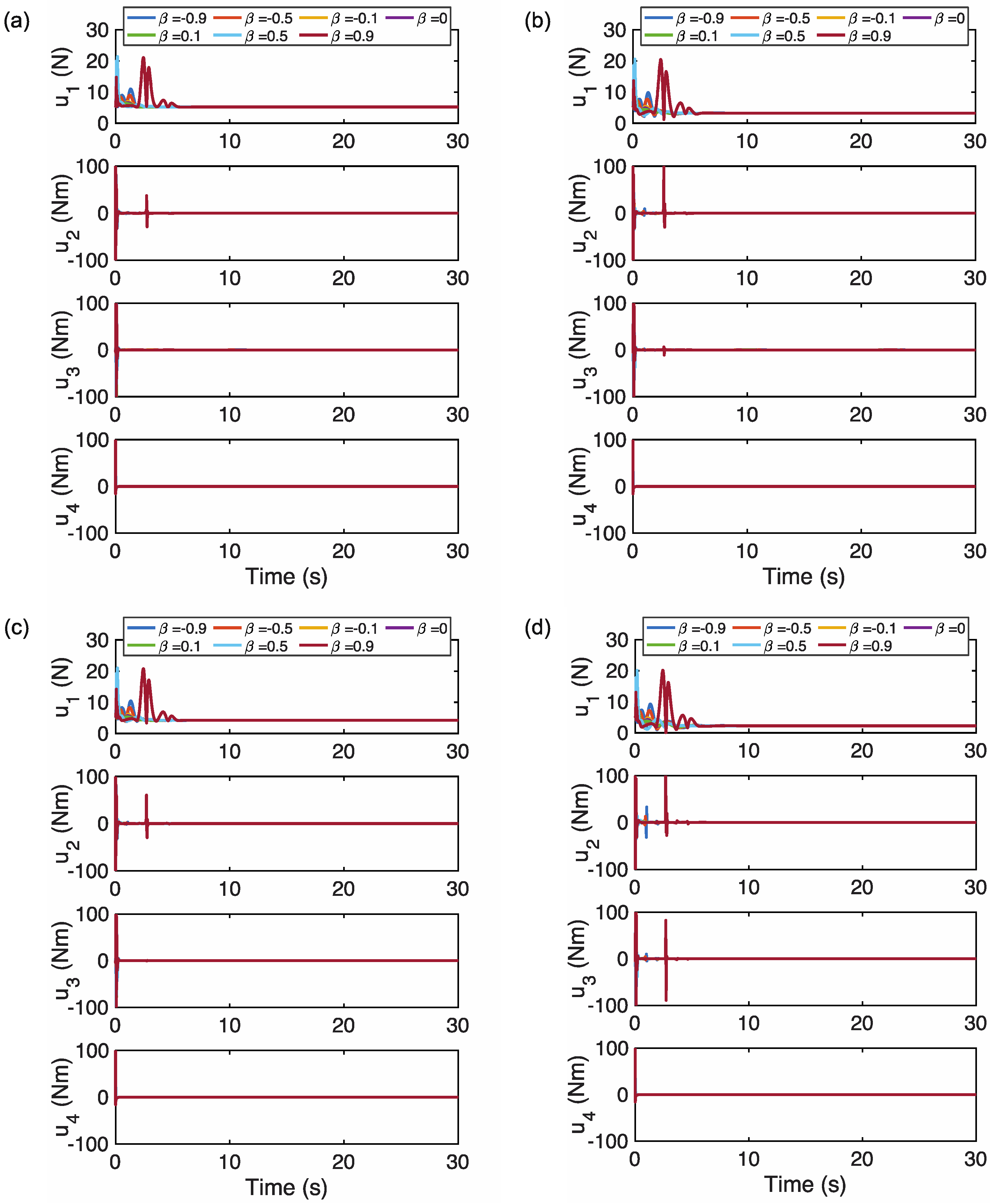
Correspondingly, the simulated control signals of varying fractional orders in the proposed RBF-ADFOBC controller in response to four different external loads are demonstrated in Figure 4, and the root mean squared values of the four control signals in the first 30 s are presented in Table 4, Table 5, Table 6 and Table 7. As the fractional order increases, the control input increases and reaches its maximum at β = 0.9 . This trend aligns with the evolving RMSE of the tracking accuracy, where higher accuracy requires higher control effort.

5.2. Closed-Loop Simulation with Unknown Input Delays

Since the Pade’s approximation in Equation (16) is only valid for small time delays, the numerical simulations in this section target the quadrotor systems with two small time delays, i.e., τ = 0.05 s and τ = 0.1 s. The simulated trajectories of the quadrotor with the controller having the two time delays at different fractional orders are shown in Figure 5. Moreover, the RMSE of the simulated trajectory with respect to the desired path in these different scenarios are presented in Table 8. It has been witnessed that the RMSE and settling time gradually decreases as β increases from −0.9 to 0.1, and it follows with larger RMSEs at β = 0.5 and β = 0.9 compared to that at β = 0.1 . These findings, while preliminary, suggest that the trajectory with the smallest RMSE can be achieved by the controller with its fractional order located at some value between 0.1 and 0.5 . In addition, an interesting observation from Table 8 is that the controller with small β values (e.g., β = 0.9 and β = 0.5 ) can demonstrate enhanced robustness to uncertain input time delays, since at these two β values, smaller RMSEs can be achieved at larger time delays. This phenomenon may be attributed to the fact that the convolution operation in higher-order fractional integrals allows the heavy-tailed kernel function (i.e., 1 / t 1 + β with β 0.5 ) to weight z1 over a wider time domain, which results in a larger virtual control α 1 at larger time delays.
Similarly, the control signals of the proposed RBF-ADFOBC controller in response to varying fractional orders and two time delays are obtained, as demonstrated in Figure 6. The root mean squared values of the control signals during the initial 30 s are provided in Table 9, Table 10, Table 11 and Table 12. The results also show that the control input has a tendency to increase with increasing fractional order and reaches its global peak at β = 0.9 . Although the root mean squared values of the control signals reach a local maximum at β = 0.9 , it should be noted that the RBF-ADFOBC with this fractional order has a significantly smaller action time region (<0.5 s) compared to the RBF-ADFOBC with other fractional orders. As a result, the RMSE of the simulated trajectory remains higher than those with other fractional orders. Furthermore, the simulated trajectory and control signal data reveal that while the maximum control effort occurs at β = 0.9 , the RMSE of the simulated trajectory at this fractional order is not necessarily the smallest. The reason is that the system stability cannot be ensured at larger positive β values, as shown in Theorem 1.

5.3. Closed-Loop Simulation with Modleing Uncertainties and Unknown Input Delays

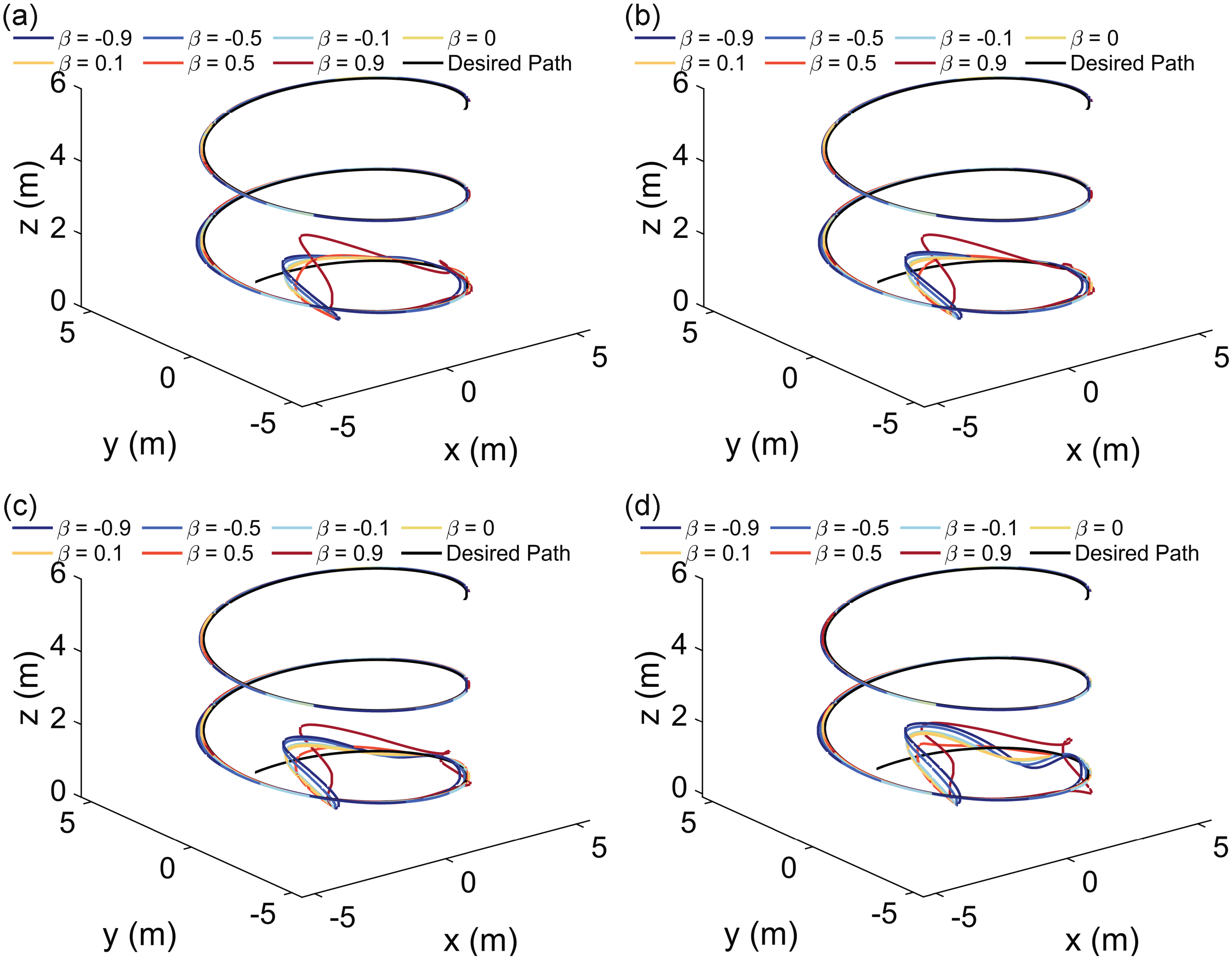
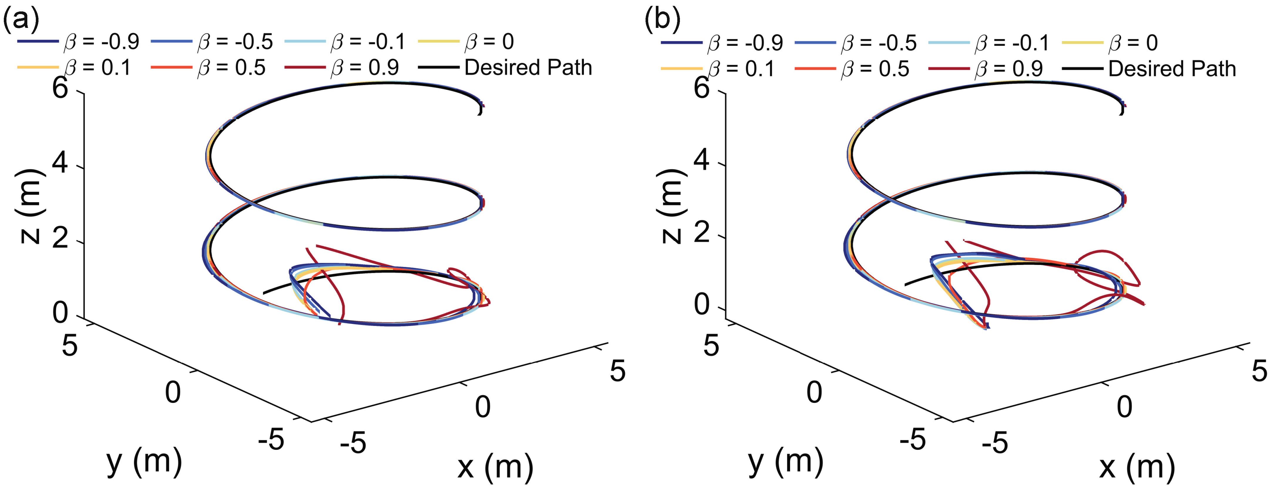
In the last set of numerical simulations, both the modeling uncertainties and input time delays are present in the quadrotor system. The simulated trajectories and the RMSEs with respect to the desired path are given in Figure 7 and Table 13, respectively. It can be seen that for either payload, the controller with β = 0.5 and β = 0.1 renders the smallest RMSEs in scenarios with τ = 0.05 s and τ = 0.1 s, respectively. In contrast to the integer-order adaptive backstepping control, the fractional-order controllers with β = 0.5 and β = 0.1 can reduce the RMSE of the tracking path by 3.7% and 2.2%, respectively. It indicates that the adaptive fractional-order control laws developed in this work can effectively improve the tracking accuracy and enhance the robustness to the co-existence of the modeling uncertainties and the uncertain input time delays at the same time. However, it can be found that the closed-loop system with β = 0.9 loses its stability when a payload of 4 m/s2 and τ = 0.1 s is considered. This observation is consistent with the implication of Theorem 1 that the stability of fractional-order controllers with large positive β values may not be guaranteed in this work.
Subsequently, Figure 8 demonstrates the control signals of the proposed RBF-ADFOBC controller in response to varying fractional orders and the presence of input delays and external payloads. Table 14, Table 15, Table 16 and Table 17 provide the root mean squared values of the control signals during the initial 30 s. The results reveal that the control input tends to increase with increasing fractional order and reaches its global peak at β = 0.9 , which is a similar consequence as the previous two sets of numerical simulations. Nonetheless, it is crucial to note that when the quadrotor is subject to a payload of 2 m/s2 and an input delay of 0.10 s, the control signal at β = 0.9 experiences an explosion, leading to the destabilization of the closed-loop system.

6. Comparison to Other Controllers

In the previous section, the simulation results of the RBF-ADFOBC with seven fractional orders have been compared, revealing that the RBF-ADFOBC with β = 0.5 (or β = 0.1) can demonstrate the best path tracking accuracy and robustness to modeling uncertainties and input time delays. In this section, the RBF-ADFOBC approach is further compared with two previous controllers to highlight the effectiveness and robustness of our RBF-ADFOBC approach. The two previous controllers include a fractional-order PID (FOPID) controller with its five parameters optimized via the particle swarm optimization (PSO) algorithm [37], and a linear quadratic regulator (LQR) controller [40]. The FOPID controller (or the LQR controller) is employed in the inner loop responsible for attitude control, as well as the outer loop tasked with position control of the quadrotor system. The transfer function of the FOPID controller is given as:
C ( s ) = K p + K i s λ + K d s μ
where K p , K i and K d are three gains of the FOPID controller, and λ and μ are the fractional orders of the integral and derivative terms, with 0 < λ , μ < 2 .
The feedback gain of the LQR controller is defined as K = R 1 B T P , where R is a positive weight parameter, B is the coefficient matrix associated with the input of the linearized state-space model of a quadrotor subsystem, and P is a positive-definite matrix that is the unique solution to the algebraic Riccati equation (ARE), ATP + PAPBR−1BTP + Q = 0, with A being the coefficient matrix of the linearized quadrotor model and Q being a positive-definite weight matrix. In [40], to mitigate the impact of perturbations and address the issue of steady-state error, the LQR controller was augmented with an integrator. Thus, the difference between the system output and the reference signal is expressed as the time derivative of an augmented state-space variable, resulting from the inclusion of a referred integrator, denoted by the symbol ξ. Then, the augmented state-space model of the position subsystem in the z direction is:
[ x ˙ 5 x ˙ 6 ξ ˙ ] = A ˜ [ x 5 x 6 ξ ] + B ˜ u z  
where A ˜ and B ˜ are the augmented coefficient matrix of the subsystem. Consider the output of the subsystem y = x 5 , and that ξ ˙ = x 5 d y , the augmented coefficient matrices are thus given by:
A ˜ = [ 0 1 0 0 0 0 1 0 0 ] ,     B ˜ = [ 0 1 / m 0 ]  
Accordingly, the augmented coefficient matrices of other subsystems can be derived in a similar way. In this work, the Q and R matrices along with the resulting optimal gains of the LQR controller are given in Table 18.
In addition, the PSO-rendered optimal parameters for the FOPID controller are given as K p = 4.0124 , K i = 3.3088 , K d = 2.9811 , λ = 0.6861 and μ = 1.1786 . To maintain presentation simplicity, we have exclusively conducted the third group of numerical simulations outlined in Section 5 for these two supplementary controllers, and the comparison of the simulated trajectories is presented in Figure 9. Meanwhile, the RMSE of the simulated trajectories rendered by the three different controllers is given in Table 19. In this section, we investigated the performance of three controllers, the optimized FOPID controller, the LQR controller, and our RBF-ADFOBC controller, under different settings of external loads and input time delays. Our results demonstrate that RBF-ADFOBC with a β value of 0.5 achieves significantly higher tracking accuracy than both the FOPID and LQR controllers, with improvements of at least 32.3% and 6%, respectively. While all three controllers maintain stability in the quadrotor system under the simulated settings, they exhibit different levels of robustness to the external loads and input time delays. Specifically, the RMSE of the simulated trajectories increases by 1.43%, 268.8% and 4.6% for FOPID, LQR and RBF-ADFOBC, respectively. Our findings suggest that the optimal FOPID controller may demonstrate the best robustness among the three controllers, possibly due to its five parameters being optimized through particle swarm optimization within a feasible parameter domain, while the parameters of the other two controllers were obtained through limited trial and error. However, despite potentially lower robustness, the RBF-ADFOBC still outperforms FOPID in terms of tracking accuracy.
A comparison is also given for the control signals of the three controllers. As shown in Figure 10 and Table 20, the root mean squared value of the first control signal u 1 in our RBF-ADFOBC controller is only 0.5% higher than that of the optimal FOPID controller, while it is 87% less than that of the LQR controller. Similar observations were made for the other three control signals. These results indicate that the optimal FOPID controller has superior control efficacy over the other three controllers. Our comparison further highlights the remarkable trajectory-tracking capability and relatively excellent control efficiency of the RBF-ADFOBC controller. Moreover, it underscores the effectiveness of fractional-order controllers in contrast to their integer-order counterparts.

7. Conclusions

In this paper, a radial basis function neural network-based adaptive fractional-order backstepping controller (RBF-ADFOBC) is proposed to achieve the robust trajectory tracking and attitude control of uncertain quadrotors with unknown input time delays. For every subsystem in the quadrotor dynamics, a compensation system and Lyapunov function are developed to guarantee the semi-globally uniformly ultimately boundedness of all the state variables and the estimation error of the uncertain parameters. Numerical simulations have been given to demonstrate the trajectory tracking accuracy and robustness of the proposed controller to the modeling uncertainties and the unknown input time delays. It has been found that the tracking error (RMSE) and settling time decrease as the fractional order β increases from −0.9 to some positive value, and the RMSE and settling time will then increase as β increases from that positive value to 0.9. In our case (with controllers evaluated at seven different β values), the best trajectory tracking performance is achieved at β = 0.1 or β = 0.5 . In contrast to the conventional (integer-order) adaptive backstepping controller (i.e., β = 0 ), the fractional-order controllers with β = 0.5 and β = 0.1 can reduce the RMSE by more than 3.7% and 2.2%, respectively, when the quadrotor is under the presence of two different payloads and input time delays. Further comparison simulations reveal that the RBF-ADFOBC controller with β = 0.5 achieved significantly higher tracking accuracy compared to the optimized FOPID and LQR controllers, with improvements of at least 32.3% and 6%, respectively, while all three controllers maintained stability. The optimal FOPID controller demonstrated the best robustness, but RBF-ADFOBC still outperformed FOPID in terms of tracking accuracy and exhibited relatively excellent control efficiency.
This work greatly enriches fractional-order adaptive control theory. The accuracy and robustness of a novel adaptive fractional-order backstepping controller is evaluated using the control of a quadrotor UAV, which is widely used in engineering and military applications, and the related theory will be extended to the control of higher-order coupled nonlinear systems as well as fractional-order systems in the next stage.

Author Contributions

Conceptualization, Y.Y.; Data curation, Y.Y.; Formal analysis, Y.Y.; Funding acquisition, H.H.Z.; Investigation, Y.Y.; Methodology, Y.Y.; Project administration, H.H.Z.; Resources, H.H.Z.; Software, Y.Y.; Supervision, H.H.Z.; Validation, Y.Y.; Visualization, Y.Y.; Writing—original draft, Y.Y.; Writing—review & editing, Y.Y. and H.H.Z. All authors have read and agreed to the published version of the manuscript.

Funding

Publication of this article was funded in part by Purdue University Libraries Open Access Publishing Fund.

Data Availability Statement

All data included in this study is self-contained in the manuscript and also available upon request via contact with the corresponding author.

Conflicts of Interest

The authors declare no conflict of interest.

Appendix A

In the RBF NN, the estimate of the weight vector W ^ 1 can be updated from the feedback θ ^ 11 . Here, | | W ^ 1 | | = b 1 θ ^ 11 is given, the input y 1 and output F 1 e = λ 1 τ 1 y 1 / 2 to the RBF NN are also given, the goal is to find W ^ 1 , such that the approximation error | | F 1 F 1 e | | is minimized, where F 1 = W ^ 1 T S 1 . That is,
W ^ 1 = arg min W 1 G | | W 1 T S 1 λ 1 τ 1 y 1 / 2 | | Subject   to   | | W ^ 1 | | = b 1 θ ^ 11
To solve this problem, a Lagrange multiplier λ is introduced and an augmented equation is given as:
f ( W 1 , λ ) = ( W 1 T S 1 λ 1 τ 1 y 1 / 2 ) T ( W 1 T S 1 λ 1 τ 1 y 1 / 2 ) λ ( | | W 1 | | 2 b 1 θ ^ 11 )
Then, taking the first partial derivatives of f yields:
f W 1 = 2 ( W 1 T S 1 λ 1 τ 1 y 1 / 2 ) S 1 2 λ W 1 = 0
f λ = | | W 1 | | 2 b 1 θ ^ 11 = 0
From Equations (A3) and (A4), the RBF approximated W ^ 1 can be obtained. Consider that the RBF NN has five radial basis nodes in this work, we can easily obtain the generic formulas for the five components of W ^ 1 5 by using the syms toolbox in Matlab. Similar procedures apply to RBF NN2 F 2 ( α 1 ) and other RBF NNs used in the controller.

Appendix B

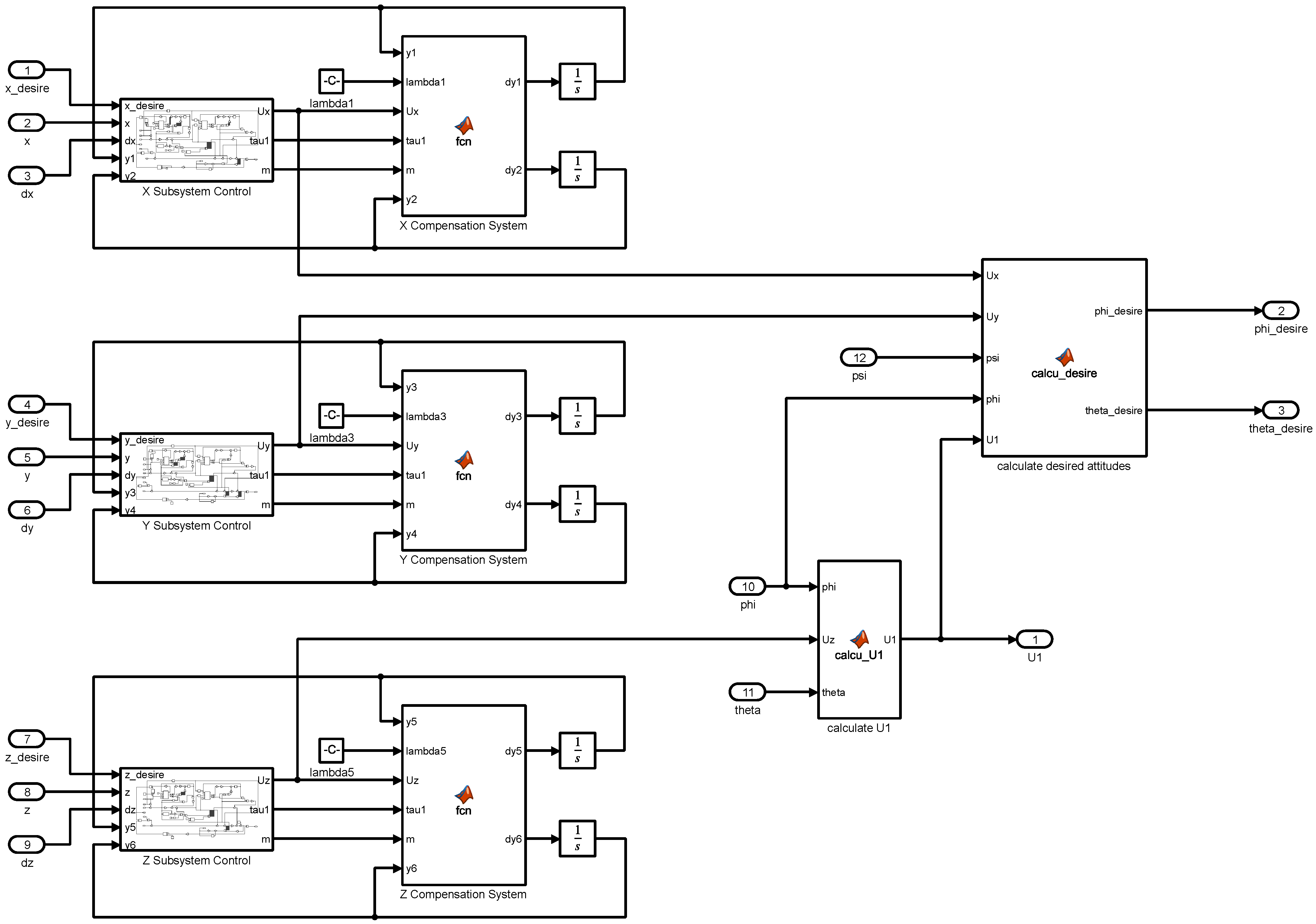
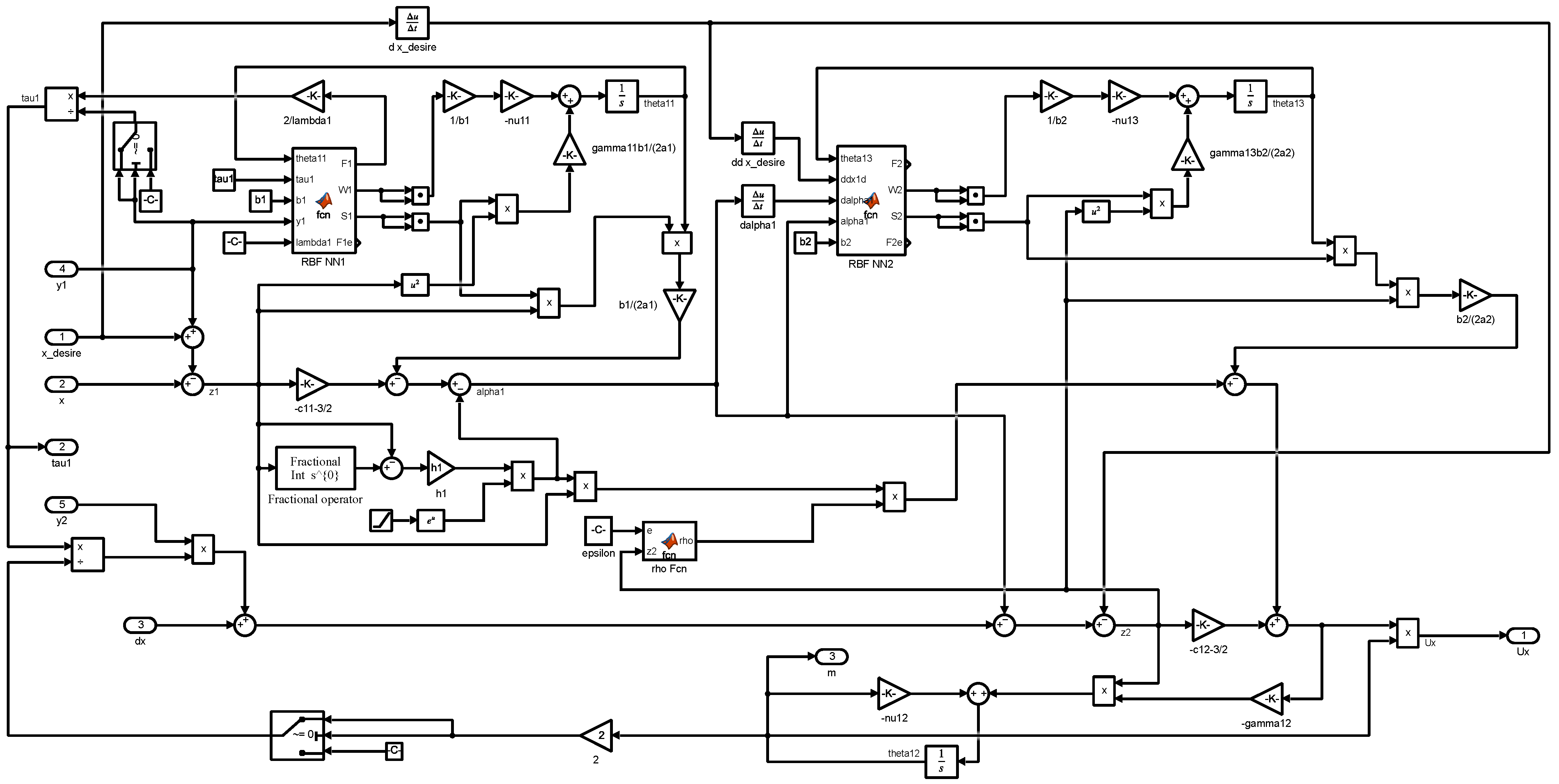
The Simulink diagram of the proposed controller is shown in Figure A1. The Simulink diagram of the position controller block is shown in Figure A2, and the expanded implementation of the X subsystem control is shown in Figure A3. The implementation for the attitude controller is omitted as it has the same internal structure as that of the position controller.
Figure A1. Simulink diagram of the closed-loop quadrotor UAV system with the proposed neural network-based adaptive fractional-order backstepping controller.
Fractalfract 07 00232 g0a1
Figure A2. Simulink diagram of the position controller.
Fractalfract 07 00232 g0a2
Figure A3. Simulink diagram of the X subsystem control block in the position controller.
Fractalfract 07 00232 g0a3

References

  1. Özbek, N.S.; Önkol, M.; Efe, M.Ö. Feedback control strategies for quadrotor-type aerial robots: A survey. Trans. Inst. Meas. Control 2015, 38, 529–554. [Google Scholar] [CrossRef]
  2. Jarray, R.; Al-Dhaifallah, M.; Rezk, H.; Bouallègue, S. Path planning of quadrotors in a dynamic environment using a multicriteria multi-verse optimizer. Comput. Mater. Contin. 2021, 69, 2159–2180. [Google Scholar] [CrossRef]
  3. Rosser, J.C.; Vignesh, V.; Terwilliger, B.A.; Parker, B.C. Surgical and medical applications of drones: A comprehensive review. J. Soc. Laparoendosc. Surg. 2018, 22, e2018.00018. [Google Scholar] [CrossRef] [Green Version]
  4. Wannberg, M. The Quadrotor Platform: From a Military Point of View; KTH Royal Institute of Technology: Stockholm, Sweden, 2012. [Google Scholar]
  5. Dhadekar, D.D.; Sanghani, P.D.; Mangrulkar, K.K.; Talole, S.E. Robust control of quadrotor using uncertainty and disturbance estimation. J. Intell. Robot. Syst. Theory Appl. 2021, 101, 60. [Google Scholar] [CrossRef]
  6. Nguyen, A.T.; Xuan-Mung, N.; Hong, S.K. Quadcopter adaptive trajectory tracking control: A new approach via backstepping technique. Appl. Sci. 2019, 9, 3873. [Google Scholar] [CrossRef] [Green Version]
  7. Sankaranarayanan, V.N.; Satpute, S.; Nikolakopoulos, G. adaptive robust control for quadrotors with unknown time-varying delays and uncertainties in dynamics. Drones 2022, 6, 220. [Google Scholar] [CrossRef]
  8. Mofid, O.; Mobayen, S.; Zhang, C.; Esakki, B. Desired tracking of delayed quadrotor UAV under model uncertainty and wind disturbance using adaptive super-twisting terminal sliding mode control. ISA Trans. 2022, 123, 455–471. [Google Scholar] [CrossRef]
  9. Li, J.; Li, Y. Dynamic analysis and PID control for a quadrotor. In Proceedings of the IEEE International Conference on Mechatronics and Automation (ICMA 2011), Beijing, China, 7–10 August 2011; IEEE: Beijing, China, 2011; pp. 573–578. [Google Scholar]
  10. Xu, R.; Özgüner, Ü. Sliding mode control of a quadrotor helicopter. In Proceedings of the IEEE Conference on Decision and Control, San Diego, CA, USA, 13–15 December 2006; IEEE: San Diego, CA, USA, 2006; pp. 4957–4962. [Google Scholar]
  11. Madani, T.; Benallegue, A. Backstepping control for a quadrotor helicopter. In Proceedings of the IEEE International Conference on Intelligent Robots and Systems, Beijing, China, 9–15 October 2006; IEEE: Beijing, China, 2006; pp. 3255–3260. [Google Scholar]
  12. Dierks, T.; Jagannathan, S. Neural network control of quadrotor UAV formations. In Proceedings of the American Control Conference, St. Louis, MO, USA, 10–12 June 2009; IEEE: St. Louis, MO, USA, 2009; pp. 2990–2996. [Google Scholar]
  13. Vaidyanathan, S. Adaptive integral sliding mode controller design for the control and synchronization of a novel jerk chaotic system. In Applications of Sliding Mode Control in Science and Engineering. Studies in Computational Intelligence; Springer: Cham, Switzerland, 2017; Volume 709, pp. 393–417. [Google Scholar]
  14. Jiang, B.; Liu, D.; Karimi, H.R.; Li, B. RBF neural network sliding mode control for passification of nonlinear time-varying delay systems with application to offshore cranes. Sensors 2022, 22, 5253. [Google Scholar] [CrossRef] [PubMed]
  15. Nguyen, N.P.; Mung, N.X.; Thanh, H.L.N.N.; Huynh, T.T.; Lam, N.T.; Hong, S.K. Adaptive sliding mode control for attitude and altitude system of a quadcopter UAV via neural network. IEEE Access 2021, 9, 40076–40085. [Google Scholar] [CrossRef]
  16. Xuan-Mung, N.; Hong, S.K. Improved altitude control algorithm for quadcopter unmanned aerial vehicles. Appl. Sci. 2019, 9, 2122. [Google Scholar] [CrossRef] [Green Version]
  17. Xuan-Mung, N.; Hong, S.K. Robust backstepping trajectory tracking control of a quadrotor with input saturation via extended state observer. Appl. Sci. 2019, 9, 5184. [Google Scholar] [CrossRef] [Green Version]
  18. Lee, J.W.; Xuan-Mung, N.; Nguyen, N.P.; Hong, S.K. Adaptive altitude flight control of quadcopter under ground effect and time-varying load: Theory and experiments. J. Vib. Control 2023, 29, 571–581. [Google Scholar] [CrossRef]
  19. Shen, S.; Xu, J. Adaptive neural network-based active disturbance rejection flight control of an unmanned helicopter. Aerosp. Sci. Technol. 2021, 119, 107062. [Google Scholar] [CrossRef]
  20. Gao, Y.; Zhu, G.; Zhao, T. Based on backpropagation neural network and adaptive linear active disturbance rejection control for attitude of a quadrotor carrying a load. Appl. Sci. 2022, 12, 12698. [Google Scholar] [CrossRef]
  21. De Ayres Junior, F.A.C.; Da Costa Junior, C.T.; De Medeiros, R.L.P.; Junior, W.B.; Das Neves, C.C.; Lenzi, M.K.; Veroneze, G.M. A fractional order power system stabilizer applied on a small-scale generation system. Energies 2018, 11, 2052. [Google Scholar] [CrossRef] [Green Version]
  22. Podlubny, I. Fractional Differential Equations, 1st ed.; Academic Press: Cambridge, MA, USA, 1999; ISBN 9780080531984. [Google Scholar]
  23. Monje, C.A.; Chen, Y.Q.; Vinagre, B.M.; Xue, D.; Feliu, V. Fractional-Order Systems and Controls: Fundamentals and Applications; Springer Science & Business Media: Berlin, Germany, 2010. [Google Scholar]
  24. Xue, D. Fractional-Order Control Systems: Fundamentals and Numerical Implementations; De Gruyter: Berlin, Germany, 2017; ISBN 9783110497977. [Google Scholar]
  25. Yang, Y.; Zhang, H.H. Fractional Calculus with Its Applications in Engineering and Technology, 1st ed.; Morgan & Claypool Publishers LLC: San Rafael, CA, USA, 2019; Volume 3. [Google Scholar]
  26. Caponetto, R.; Tenereiro Machado, J.A.; Trujillo, J.J. Theory and applications of fractional order systems. Math. Probl. Eng. 2014, 2014, 596195. [Google Scholar] [CrossRef]
  27. Baleanu, D.; Caponetto, R.; Machado, J.T. Challenges in fractional dynamics and control theory. J. Vib. Control 2016, 22, 2151–2152. [Google Scholar] [CrossRef] [Green Version]
  28. Lopes, A.M.; Chen, L. Fractional Order Systems and Their Applications. Fractal Fract. 2022, 6, 389. [Google Scholar] [CrossRef]
  29. David, S.A.; Linares, J.L.; Pallone, E.M.J.A. Fractional order calculus: Historical apologia, basic concepts and some applications. Rev. Bras. Ensino Fis. 2011, 33, 4302. [Google Scholar] [CrossRef]
  30. Yang, Y.; Zhang, H.H.; Voyles, R.M. Rotary inverted pendulum system tracking and stability control based on input-output feedback linearization and PSO-optimized fractional order PID controller. In Automatic Control, Mechatronics and Industrial Engineering; CRC Press: Boca Raton, FL, USA, 2019; pp. 79–84. ISBN 9780429468605. [Google Scholar]
  31. Yang, Y.; Zhang, H.H.; Voyles, R.M. Optimal fractional-order proportional– integral–derivative control enabling full actuation of decomposed rotary inverted pendulum system. Trans. Inst. Meas. Control 2023, in press. [Google Scholar] [CrossRef]
  32. Yang, Y.; Zhang, H.H.; Yu, W.; Tan, L. Optimal design of discrete-time fractional-order PID controller for idle speed control of an IC engine. Int. J. Powertrains 2020, 9, 79–97. [Google Scholar] [CrossRef]
  33. Yang, Y.; Nawrocki, R.; Voyles, R.; Zhang, H.H. A fractional drift diffusion model for organic semiconductor devices. Comput. Mater. Contin. 2021, 69, 237–266. [Google Scholar] [CrossRef]
  34. Xu, K.; Cheng, T.; Lopes, A.M.; Chen, L.; Zhu, X.; Wang, M. Fuzzy fractional-order PD vibration control of uncertain building structures. Fractal Fract. 2022, 6, 473. [Google Scholar] [CrossRef]
  35. Lien, C.-H.; Chang, H.-C.; Yu, K.-W.; Li, H.-C.; Hou, Y.-Y.; Lien, C.-H.; Chang, H.-C.; Yu, K.-W.; Li, H.-C.; Hou, Y.-Y. Robust H controller design of switched delay systems with linear fractional perturbations by synchronous switching of rule and sampling input. Fractal Fract. 2022, 6, 479. [Google Scholar] [CrossRef]
  36. Xu, L.; Du, J.; Song, B.; Cao, M. A combined backstepping and fractional-order PID controller to trajectory tracking of mobile robots. Syst. Sci. Control Eng. 2022, 10, 133–140. [Google Scholar] [CrossRef]
  37. Shao, K.; Liu, J.; Li Keyong Shao, M.; Li, M. Fractional order PID control of quadrotor UAV based on SA-PSO algorithm. In Proceedings of the Third International Conference on Computer Science and Communication Technology (ICCSCT 2022), Virtual, 25–26 November 2022; Lu, Y., Cheng, C., Eds.; SPIE: Bellingham, WA, USA, 2022; Volume 12506, pp. 73–81. [Google Scholar]
  38. Labbadi, M.; Boukal, Y.; Cherkaoui, M.; Djemai, M. Fractional-order global sliding mode controller for an uncertain quadrotor UAVs subjected to external disturbances. J. Frankl. Inst. 2021, 358, 4822–4847. [Google Scholar] [CrossRef]
  39. Timis, D.D.; Muresan, C.I.; Dulf, E.H. Design and experimental results of an adaptive fractional-order controller for a quadrotor. Fractal Fract. 2022, 6, 204. [Google Scholar] [CrossRef]
  40. Martins, L.; Cardeira, C.; Oliveira, P. Linear quadratic regulator for trajectory tracking of a quadrotor. IFAC-Pap. 2019, 52, 176–181. [Google Scholar] [CrossRef]
  41. Oustaloup, A. La Dérivation non Entière: Théorie, Synthèse et Applications; Hermes: Paris, France, 1995; ISBN 9782866014568. [Google Scholar]
  42. Moody, J.; Darken, C.J. Fast learning in networks of locally-tuned processing units. Neural Comput. 1989, 1, 281–294. [Google Scholar] [CrossRef]
  43. Khanesar, M.A.; Kaynak, O.; Yin, S.; Gao, H. Adaptive indirect fuzzy sliding mode controller for networked control systems subject to time-varying network-induced time delay. IEEE Trans. Fuzzy Syst. 2015, 23, 205–214. [Google Scholar] [CrossRef]
  44. Obuz, S.; Klotz, J.R.; Kamalapurkar, R.; Dixon, W. Unknown time-varying input delay compensation for uncertain nonlinear systems. Automatica 2017, 76, 222–229. [Google Scholar] [CrossRef]
  45. Deng, W.; Yao, J.; Ma, D. Time-varying input delay compensation for nonlinear systems with additive disturbance: An output feedback approach. Int. J. Robust Nonlinear Control 2018, 28, 31–52. [Google Scholar] [CrossRef]
  46. Li, H.; Wang, L.; Du, H.; Boulkroune, A. Adaptive fuzzy backstepping tracking control for strict-feedback systems with input delay. IEEE Trans. Fuzzy Syst. 2017, 25, 642–652. [Google Scholar] [CrossRef]
Figure 3. Simulated results that demonstrate the robustness of the varying fractional orders in the proposed controller to uncertainty in the quadrotor dynamics with various payloads: (a) d 3 = 0 m/s2, (b) d 3 = 2 m/s2, (c) d 3 = 4 m/s2, (d) d 3 = 6 m/s2. (Assume that d 1 = d 2 = d 4 = d 5 = d 6 = 0 and no input time delay.)
Fractalfract 07 00232 g003
Figure 4. Simulated control inputs of the varying fractional orders in the proposed controller to uncertainty in the quadrotor dynamics with various payloads: (a) d 3 = 0 m/s2, (b) d 3 = 2 m/s2, (c) d 3 = 4 m/s2, (d) d 3 = 6 m/s2. (Assume that d 1 = d 2 = d 4 = d 5 = d 6 = 0 and no input time delay.)
Fractalfract 07 00232 g004
Figure 5. Simulated results that demonstrate the robustness of the varying fractional orders in the proposed controller to various input delays: (a) τ = 0.05 s, (b) τ = 0.1 s. (Assume that τ = τ 1 = τ 2 = τ 3 = τ 4 and no payload is applied.)
Fractalfract 07 00232 g005
Figure 6. Simulated control inputs of the varying fractional orders in the proposed controller to various input delays: (a) τ = 0.05 s, (b) τ = 0.1 s. (Assume that τ = τ 1 = τ 2 = τ 3 = τ 4 and no payload is applied.)
Fractalfract 07 00232 g006
Figure 7. Simulated results that demonstrate the robustness of the varying fractional orders in the proposed controller to uncertainty in the quadrotor dynamics with various payloads and uncertain input time delays: (a) d 3 = 2 m/s2 and τ = 0.05 s, (b) d 3 = 2 m/s2 and τ = 0.10 s, (c) d 3 = 4 m/s2 and τ = 0.05 s, (d) d 3 = 4 m/s2 and τ = 0.10 s. (Assume that d 1 = d 2 = d 4 = d 5 = d 6 = 0 and τ = τ 1 = τ 2 = τ 3 = τ 4 .)
Fractalfract 07 00232 g007
Figure 8. Simulated control inputs of the varying fractional orders in the proposed controller to uncertainty in the quadrotor dynamics with various payloads and uncertain input time delays: (a) d 3 = 2 m/s2 and τ = 0.05 s, (b) d 3 = 2 m/s2 and τ = 0.10 s, (c) d 3 = 4 m/s2 and τ = 0.05 s, (d) d 3 = 4 m/s2 and τ = 0.10 s. (Assume that d 1 = d 2 = d 4 = d 5 = d 6 = 0 and τ = τ 1 = τ 2 = τ 3 = τ 4 .)
Fractalfract 07 00232 g008
Figure 9. Comparison of the simulated trajectories with three controllers ( β = 0.5 in RBF-ADFOBC) in response to various payloads and uncertain input time delays: (a) d 3 = 2 m/s2 and τ = 0.05 s, (b) d 3 = 2 m/s2 and τ = 0.10 s, (c) d 3 = 4 m/s2 and τ = 0.05 s, (d) d 3 = 4 m/s2 and τ = 0.10 s. (Assume that d 1 = d 2 = d 4 = d 5 = d 6 = 0 and τ = τ 1 = τ 2 = τ 3 = τ 4 .)
Fractalfract 07 00232 g009
Figure 10. Comparison of the simulated control signals with three controllers ( β = 0.5 in RBF-ADFOBC) in response to various payloads and uncertain input time delays: (a) d 3 = 2 m/s2 and τ = 0.05 s, (b) d 3 = 2 m/s2 and τ = 0.10 s, (c) d 3 = 4 m/s2 and τ = 0.05 s, (d) d 3 = 4 m/s2 and τ = 0.10 s. (Assume that d 1 = d 2 = d 4 = d 5 = d 6 = 0 and τ = τ 1 = τ 2 = τ 3 = τ 4 .)
Fractalfract 07 00232 g010
Table 2. Values for the selectable parameters in the proposed controllers.
ParamValueParamValueParamValueParamValueParamValue
a 1 5 a 2 5 b 1 1 b 2 1 c 11 5
c 12 5 γ 11 10 γ 12 10 γ 13 10 ν 11 10
ν 12 10 ν 13 10 h 1 2 r 1 0.1 λ 1 2
a 3 5 a 4 5 b 3 1 b 4 1 c 31 5
c 32 5 γ 31 10 γ 32 10 γ 33 10 ν 31 10
ν 32 10 ν 33 10 h 3 2 r 3 0.1 λ 3 2
a 5 5 a 6 5 b 5 1 b 6 1 c 51 5
c 52 5 γ 51 10 γ 52 10 γ 53 10 ν 51 10
ν 52 10 ν 53 10 h 5 2 r 5 0.1 λ 5 2
a 7 5 a 8 5 b 7 1 b 8 1 c 71 5
c 72 5 γ 71 10 γ 72 10 γ 73 10 ν 71 10
ν 72 10 ν 73 10 h 7 2 r 7 0.1 λ 7 2
a 9 5 a 10 5 b 9 1 b 10 1 c 91 5
c 92 5 γ 91 10 γ 92 10 γ 93 10 ν 91 10
ν 92 10 ν 93 10 h 9 2 r 9 0.1 λ 9 2
a 11 5 a 12 5 b 11 1 b 12 1 c 111 5
c 112 5 γ 111 10 γ 112 10 γ 113 10 ν 111 10
ν 112 10 ν 113 10 h 11 2 r 11 0.1 λ 11 2
Table 3. Root mean squared error (RMSE) of the simulated tracks under different payloads and different fractional orders in the proposed controller.
Payloads (m/s2) β = 0.9 β = 0.5 β = 0.1 β = 0 β = 0.1 β = 0.5 β = 0.9
00.64930.59630.51270.49530.48300.47860.7251
20.64590.59430.51320.49620.48410.48000.7241
40.63870.59000.51290.49640.48460.48060.7208
60.62950.58420.51190.49610.48470.48020.7139
Table 4. Root mean squared value of the control signal u 1 in the first 30 s under different payloads and different fractional orders in the proposed controller.
Payloads (m/s2) β = 0.9 β = 0.5 β = 0.1 β = 0 β = 0.1 β = 0.5 β = 0.9
05.43615.37135.33445.34295.35305.38575.9943
24.48244.40714.36384.37334.38484.42145.1261
43.55543.46523.41223.42343.43693.47964.3215
62.69002.57642.50652.51962.53542.58493.6169
Table 5. Root mean squared value of the control signal u 2 in the first 30 s under different payloads and different fractional orders in the proposed controller.
Payloads (m/s2) β = 0.9 β = 0.5 β = 0.1 β = 0 β = 0.1 β = 0.5 β = 0.9
02.01061.58321.90392.36512.42812.52675.6396
22.02571.60091.93992.37532.43592.53595.6718
42.06231.62881.97382.38622.44472.54605.7331
62.23291.70232.00952.39902.45472.55925.8290
Table 6. Root mean squared value of the control signal u 3 in the first 30 s under different payloads and different fractional orders in the proposed controller.
Payloads (m/s2) β = 0.9 β = 0.5 β = 0.1 β = 0 β = 0.1 β = 0.5 β = 0.9
04.50574.01874.78544.79794.82034.82166.1584
24.51584.03174.80054.80294.82294.82256.1636
44.52644.04364.81384.80684.82424.82246.1761
64.54764.06094.82644.81024.82494.82246.4069
Table 7. Root mean squared value of the control signal u 4 in the first 30 s under different payloads and different fractional orders in the proposed controller.
Payloads (m/s2) β = 0.9 β = 0.5 β = 0.1 β = 0 β = 0.1 β = 0.5 β = 0.9
00.38470.38510.38710.38840.39030.42072.3505
20.38470.38510.38710.38840.39030.42072.3505
40.38470.38510.38710.38840.39030.42072.3505
60.38470.38510.38710.38840.39030.42072.3505
Table 8. Root mean squared error (RMSE) of the simulated tracks under different input time delays and different fractional orders in the proposed controller.
τ (s) β = 0.9 β = 0.5 β = 0.1 β = 0 β = 0.1 β = 0.5 β = 0.9
0.050.64840.59260.51870.50220.48980.48360.7429
0.100.63800.58550.52920.51500.50400.50750.7923
Table 9. Root mean squared value of the control signal u 1 in the first 30 s under different input time delays and different fractional orders in the proposed controller.
τ (s) β = 0.9 β = 0.5 β = 0.1 β = 0 β = 0.1 β = 0.5 β = 0.9
0.055.44115.37875.35415.36855.38295.44506.4784
0.105.47215.39845.37655.38305.39755.46497.4987
Table 10. Root mean squared value of the control signal u 2 in the first 30 s under different input time delays and different fractional orders in the proposed controller.
τ (s) β = 0.9 β = 0.5 β = 0.1 β = 0 β = 0.1 β = 0.5 β = 0.9
0.051.93311.50501.68912.31412.37882.54565.6385
0.101.92891.48891.61402.30262.36202.466513.3469
Table 11. Root mean squared value of the control signal u 3 in the first 30 s under different input time delays and different fractional orders in the proposed controller.
τ (s) β = 0.9 β = 0.5 β = 0.1 β = 0 β = 0.1 β = 0.5 β = 0.9
0.054.43773.93164.69764.79504.85024.96016.1635
0.104.41853.88994.66364.75694.81494.885315.0158
Table 12. Root mean squared value of the control signal u 4 in the first 30 s under different input time delays and different fractional orders in the proposed controller.
τ (s) β = 0.9 β = 0.5 β = 0.1 β = 0 β = 0.1 β = 0.5 β = 0.9
0.050.38420.38460.38660.38790.38850.42272.3533
0.100.38390.38410.38620.38730.38820.42232.3530
Table 13. Root mean squared error (RMSE) of the simulated tracks under different payloads, different input time delays and different fractional orders in the proposed controller.
Payloads (m/s2) τ (s) β = 0.9 β = 0.5 β = 0.1 β = 0 β = 0.1 β = 0.5 β = 0.9
20.050.64930.59440.51920.50270.49030.48430.7422
0.100.64360.58920.52980.51510.50400.50640.8158
40.050.64740.59420.51900.50250.49020.48440.7410
0.100.64470.59020.52960.51470.50370.5048116.7240
Table 14. Root mean squared value of the control signal u 1 in the first 30 s under different payloads, different input time delays and different fractional orders in the proposed controller.
Payloads (m/s2) τ (s) β = 0.9 β = 0.5 β = 0.1 β = 0 β = 0.1 β = 0.5 β = 0.9
20.054.49594.41874.38814.40584.42314.49695.7538
0.104.54434.44614.41624.42484.44224.528517.8763
40.054.03473.94763.91263.93233.95154.03285.4364
0.104.09413.98133.94543.95473.97364.07319850.6
Table 15. Root mean squared value of the control signal u 2 in the first 30 s under different payloads, different input time delays and different fractional orders in the proposed controller.
Payloads (m/s2) τ (s) β = 0.9 β = 0.5 β = 0.1 β = 0 β = 0.1 β = 0.5 β = 0.9
20.051.95051.52001.73072.32332.39122.58395.6791
0.101.96811.50591.70892.31232.36912.597026.4734
40.051.96921.53151.75402.32932.40052.61005.7090
0.102.29841.52671.74382.31972.37812.632560.9009
Table 16. Root mean squared value of the control signal u 3 in the first 30 s under different payloads, different input time delays and different fractional orders in the proposed controller.
Payloads (m/s2) τ (s) β = 0.9 β = 0.5 β = 0.1 β = 0 β = 0.1 β = 0.5 β = 0.9
20.054.44853.94364.72164.80834.86374.96366.1716
0.104.42913.90224.68444.77174.82614.923627.0198
40.054.45403.95074.73414.81524.87234.96496.1762
0.104.44023.90894.69604.77934.83214.933267.0480
Table 17. Root mean squared value of the control signal u 4 in the first 30 s under different payloads, different input time delays and different fractional orders in the proposed controller.
Payloads (m/s2) τ (s) β = 0.9 β = 0.5 β = 0.1 β = 0 β = 0.1 β = 0.5 β = 0.9
20.050.38350.38400.38550.38750.38920.42072.3505
0.100.38450.38490.38660.38830.39000.42112.3509
40.050.38500.38550.38750.38910.39050.42132.3515
0.100.38520.38660.38770.38990.39310.42222.3520
Table 18. Q and R matrices used in the LQR optimal gain calculation and the resulting optimal gains for each subsystem.
Subsystem Q R K
X Position ( x 1 )diag(1000, 20, 100)3[19.8524, 5.2640, −5.7735]
Y Position ( x 3 )diag(1000, 20, 100)3[19.8524, 5.2640, −5.7735]
Z Position ( x 5 )diag(1000, 20, 100)3[19.8524, 5.2640, −5.7735]
Roll Angle ( x 7 )diag(1000, 20, 100)3[19.0702, 2.6276, −5.7735]
Pitch Angle ( x 9 )diag(1000, 20, 100)3[19.0702, 2.6276, −5.7735]
Yaw Angle ( x 11 )diag(1000, 20, 100)3[19.0811, 2.6635, −5.7735]
Table 19. Root mean squared error (RMSE) of the simulated tracks under different payloads and different input time delays for the three different controllers.
Payloads (m/s2) τ (s)FOPIDLQR RBF ADFOBC   ( β = 0.5 )
20.050.75800.51550.4843
0.100.74800.59880.5064
40.050.76230.51990.4844
0.100.76141.90110.5048
Table 20. Comparison of the root mean squared value of the control signals in the three controllers under different payloads, different input time delays and different fractional orders.
Payloads (m/s2) τ (s)FOPIDLQR RBF ADFOBC   ( β = 0.5 )
u 1 u 2 u 3 u 4 u 1 u 2 u 3 u 4 u 1 u 2 u 3 u 4
20.054.47212.09720.63812.097734.981318.074217.083112.10744.49692.58394.96360.4207
0.104.48242.07070.80752.097755.817231.792023.889112.10744.52852.59704.92360.4211
40.053.99682.09920.64522.097729.248618.396017.163112.10744.03282.61004.96490.4213
0.104.03913.23321.29222.09771073.933.209832.398812.10744.07312.63254.93320.4222
Disclaimer/Publisher’s Note: The statements, opinions and data contained in all publications are solely those of the individual author(s) and contributor(s) and not of MDPI and/or the editor(s). MDPI and/or the editor(s) disclaim responsibility for any injury to people or property resulting from any ideas, methods, instructions or products referred to in the content.