Qualitatively Stable Schemes for the Black–Scholes Equation

Abstract

In this paper, the Black–Scholes equation is solved using a new technique. This scheme is derived by combining the Laplace transform method and the nonstandard finite difference (NSFD) strategy. The qualitative properties of the method are discussed, and it is shown that the new method is positive, stable, and consistent when low volatility is assumed. The efficiency of the new method is demonstrated by a numerical example.

1. Introduction

Derivatives are the basic pillars of financial and economic systems. The most common derivatives are options, futures, and forward contracts. Options are agreements that give the owner the possibility, not the commitment, to purchase or sell an asset at a specific price and at a specific time. These bonds are defined in two general types call options and put options. Additionally, in terms of how they are exercised, they are divided to two general types: American and European. The latter are only exercised on the maturity date, but American options may be applied at any time until the contract expires. In the financial derivatives market, fair pricing of the option is the most important issue. In the early 1970s, Black and Scholes took important steps in pricing the options. The result of their work led to the introduction of the Black–Scholes model, also famous as the Black–Scholes–Merton (BSM) model [1].

Several works are proposed for solving the BSM model. In [2], a semi-discretization method based on non-uniform grids using the second-order central finite difference is used to numerically solve the BSM model. The stability of the numerical solution is also studied. Using the Black–Scholes model, Milev and Tagliani [3] present a problem for pricing barrier options to the random movement of the asset. In this problem, choosing a similar approximation to the quadrature method for calculating an integral path is assumed. In [4], the ADE method is presented for one-factor option pricing models. Additionally, the stability, accuracy, and robust performance of this method are investigated. Golbabaei et al. [5] investigated the performance of the finite element method for option valuation. They showed that if this method is used correctly, the results of the method are superconvergent at the boundaries of the finite elements. In [6], Mehdizadeh Khalsarai and Shokri Jahandizi, an explicit method for pricing barrier options based on a non-standard discretization strategy is proposed. In their method, qualitative properties, such as positivity, stability, and compatibility, are preserved. A projection method for pricing barrier options is presented by Farnoush et al. [7]. Legendre polynomials are used as orthogonal bases in the implementation of the method. In [8], an explicit scheme to solve the BSM model without frontier data is presented. In this method, the numerical solution is calculated at each time point on the new node points, using the reduction of one or two node points. In [9], an explicit scheme is used to solve the BSM model with a hybrid boundary. In this method, a linear frontier data is used at the boundaries so that at least one asset is zero. They reduce the domain of the calculations by using a time step. Thus there is no need for boundary conditions. The Crank–Nicholson method to discretize the time for the valuation of European options and barrier options is proposed by Abdi–Mazrae et al. [10]. Then, to solve the ODE problems, the multiple shooting method with Lagrange polynomials is applied [11,12]. The error at each step is controlled by using the Crank–Nicholson method with variable step length, which prevents the propagation of error. This will lead to faster computations by increasing the step length at the smooth points of the domain. In [13], to solve the generalized Black–Scholes equation numerically, the temporal variable is discretized by the Crank–Nicholson scheme, and the spatial variable is discretized with the sextic B-spline collocation method. The method has second-order convergence with respect to the time variable and sixth-order convergence with respect to the space variable.

As the governing equation, the Black–Scholes model for pricing the European option is considered [14]:

$$-\frac{\partial v}{\partial t}+rS\frac{\partial v}{\partial S}+\frac{1}{2}{\sigma }^2{S}^2\frac{{\partial }^{2}v}{\partial S^2}-rv=0.$$

(1)

With prime and frontier data, the following

$$v(S,0)=max(S-\mathcal{K},0){\mathbf{1}}_{[\mathcal{L},\mathcal{U}]}\left(S\right),$$

(2)

$$v(S,t)\to 0asS\to 0orS\to \infty ,$$

(3)

by updating the prime data on the monitoring dates $t_i(i=0,\dots F)$

$$v(S,t_i)=v(S,t_i^{-}){\mathbf{1}}_{[\mathcal{L},\mathcal{U}]}\left(S\right),$$

(4)

where ${\mathbf{1}}_{[L,U]}$ is an indicator function and is defined as follows:

$${\mathbf{1}}_{[\mathcal{L},\mathcal{U}]}=\left\{\begin{array}{cc}\hfill 1& \mathrm{if}S\in [\mathcal{L},\mathcal{U}],\hfill \\ \hfill 0& \mathrm{if}S\notin [\mathcal{L},\mathcal{U}],\hfill \end{array}\right.$$

where $\mathcal{L}$ and $\mathcal{U}$ are lower and upper barriers actives at all times $t_n$. Moreover, S is the asset price, v the option price (a function of the underlying asset price and time), $\mathcal{K}$ the price of the strike, and T the expiration date. The payoff function of this option is equal to $max(S-\mathcal{K},0)$, but if the price of the asset falls outside the range of $[\mathcal{L},\mathcal{U}]$, the contract expires. The knock-out option at the monitoring dates indicates a discontinuity in obstacles $S=\mathcal{L}$ and $S=\mathcal{U}$, respectively.

Although standard finite difference methods (FDMs) are consistent with the principal equation and guarantee convergence, they may not maintain the qualitative behavior of the solution. In [14], a numerical method to solve (1) is presented in which a combination of the Laplace transform method and the standard FDM is used. The method produces negative values and spurious oscillations when the central differences are used to discretize first- and second-order derivatives in the case of ${\sigma }^2\ll r$.

In this paper, we modify the presented method in [14] by combining the Laplace transform method with the NSFD method. We use a non-local expression to approximate the reaction sentence in the proposed method. The new method is conditionally stable, positivity preserving and of second-order of convergence with respect to the space variable. The option price values are plotted for all time levels, which shows that the new method is positive and non-oscillating.

This paper is divided into the following sections. In Section 2, we briefly describe the Laplace transformation method. In Section 3, we apply the Laplace transformation method for the BSM equation. In Section 4, we have an overview of NSFD methods. In Section 5, we present the new method using non-local approximation for the reaction term of the BS equation. The evaluation of the novel method which pertains to the positivity-preserving property, truncation error and stability is presented in Section 6. The numerical experiments to confirm the efficiency of the new method are given in Section 7.

2. The Laplace Transform

Definition 1

([15]). Suppose $f\left(t\right)$ is a function, and its Laplace transform is defined by

$$\begin{array}{c}\hfill \mathcal{L}\left\{f\left(t\right)\right\}={\int }_0^{\infty }{e}^{-\lambda t}f\left(t\right)\mathrm{d}t,\end{array}$$

(5)

where the transform is denoted by $F\left(\lambda \right)$. Let $f\left(t\right)$ for all positive values t be defined in range $(0,\infty )$. Additionally, it is assumed that λ is real and the integral is convergent. For integral convergence (5), the following condition must hold:

$$\begin{array}{c}\hfill Re\lambda >\gamma ,\end{array}$$

where γ is a constant and $f\left(t\right)$ satisfying

$$\begin{array}{c}\hfill \left|f\left(t\right)\right|=O\left(e^{\gamma t}\right)\mathrm{as}t\to \infty .\end{array}$$

(6)

Theorem 1

([16]). Suppose $f\left(t\right)$ is a piecewise continuous function with exponential order γ on intervals $[0,\infty )$ and $\mathcal{L}\left(f\left(t\right)\right)=F\left(\lambda \right)$. Then

$$\begin{array}{c}\hfill F^{\left(k\right)}\left(\lambda \right)={(-1)}^k{\int }_0^{\infty }{t}^k{e}^{-\lambda t}f\left(t\right)\mathrm{d}t,k=1,2,3,\dots (\lambda >\gamma ).\end{array}$$

(7)

If $\mathcal{L}\left(f\left(t\right)\right)=F\left(\lambda \right)$, then the inverse Laplace transform is defined by

$$\begin{array}{c}\hfill f\left(t\right)={\mathcal{L}}^{-1}\left\{F\left(\lambda \right)\right\}.\end{array}$$

(8)

Theorem 2

((Post-Widder) [15]). If the integral

$$\begin{array}{c}\hfill \mathcal{L}\left\{f\left(t\right)\right\}={\int }_0^{\infty }{e}^{-\lambda t}f\left(t\right)\mathrm{d}t.\end{array}$$

(9)

converges for every $\lambda >\gamma$, then for every $t>0$ of continuity of $f\left(t\right)$, the inverse Laplace transform is defined as follows:

$$\begin{array}{c}\hfill f\left(t\right)=\underset{k\to \infty }{lim}\frac{{(-1)}^k}{k!}{\left(\frac{k}{t}\right)}^{k+1}{F}^{\left(k\right)}\left(\frac{k}{t}\right).\end{array}$$

(10)

The Laplace transform is a way to solve partial differential equations. In this method, by taking the Laplace transform with respect to a variable, a PDE transforms into an ODE.

For example, by taking the Laplace transform of $v(S,t)$ with respect to t, the following equation will be obtained:

$$\begin{array}{c}\hfill V(S,\lambda )={\int }_0^{\infty }{e}^{-\lambda t}v(S,t)\mathrm{d}t,\end{array}$$

(11)

where $v(S,t)$ is the solution to the PDE, and the k-th derivative of the Laplace transform is defined as follows:

$$\begin{array}{c}\hfill \frac{d^{k}V(S,\lambda )}{d{\lambda }^k}=:V^{\left(k\right)}(S,\lambda )={(-1)}^k{\int }_0^{\infty }{t}^k{e}^{-\lambda t}v(S,t)\mathrm{d}t.\end{array}$$

(12)

The Laplace transform of $v_t$ is defined as follows:

$$\begin{array}{c}\hfill \mathcal{L}\{\frac{\partial v}{\partial t}\}={\int }_0^{\infty }{e}^{-\lambda t}{v}_t(S,t)\mathrm{d}t=\lambda V(S,\lambda )-v(S,0),\end{array}$$

(13)

where $v(S,0)$ is the initial condition. Additionally, the Laplace transform of $\frac{\partial v}{\partial S}$ and $\frac{{\partial }^{2}v}{\partial S^2}$ is defined by

$$\begin{array}{c}\hfill \mathcal{L}\{\frac{\partial v}{\partial S}\}=\frac{\mathrm{d}}{\mathrm{d}S}\{\mathcal{L}\left[v(S,t)\right]\}=\frac{\mathrm{d}V(S,\lambda )}{\mathrm{d}S},\end{array}$$

(14)

and

$$\begin{array}{c}\hfill \mathcal{L}\{\frac{{\partial }^{2}v}{\partial S^2}\}=\frac{{\mathrm{d}}^2}{\mathrm{d}{S}^2}\{\mathcal{L}\left[v(S,t)\right]\}=\frac{{\mathrm{d}}^{2}V(S,\lambda )}{\mathrm{d}{S}^2},\end{array}$$

(15)

by eliminating variable t using the Laplace transform, the PDE transforms into an ODE with boundary conditions [17].

3. The Laplace Transform Method for the BSM Equation

In this section, the combination of the Laplace transform and FDM is used to numerically solve the BSM model (1). Multiplying each term of (1) by $t^k{e}^{-\lambda t}$ and integration on the interval $[0,\infty )$, we have

$$-{\int }_0^{\infty }{t}^k{e}^{-\lambda t}\frac{\partial v}{\partial t}+rS{\int }_0^{\infty }{t}^k{e}^{-\lambda t}\frac{\partial v}{\partial S}+\frac{1}{2}{\sigma }^2{S}^2{\int }_0^{\infty }{t}^k{e}^{-\lambda t}\frac{{\partial }^{2}v}{\partial S^2}-r{\int }_0^{\infty }{t}^k{e}^{-\lambda t}v=0.$$

(16)

Now, by taking the Laplace transform with respect to variable t and by using (11)–(15), the following ordinary differential equation (ODE) is obtained as follows:

$$-\frac{1}{2}{\sigma }^2{S}^2\frac{d^2{V}^{\left(k\right)}}{d{S}^2}-rS\frac{d{V}^{\left(k\right)}}{dS}+(r+\lambda )V^{\left(k\right)}=\left\{\begin{array}{ll}v(S,0),& k=0,\\ -k{V}^{(k-1)},& k=1,2,\cdots .\end{array}\right.$$

(17)

The above relative is a recursive relationship, relating two consecutive derivatives $V^{(k-1)}$ and $V^{\left(k\right)}$. Then all higher derivatives $V^{\left(k\right)}(S,\lambda )$ are obtained by an iterative procedure involving the ODE (17). Now, we can obtain the numerical solution of (17) with a finite difference method. By using the central difference for $\frac{d^2{V}^{\left(k\right)}}{d{S}^2}$ and the upwind difference for $\frac{d{V}^{\left(k\right)}}{dS}$, the following is obtained:

$$\begin{array}{cc}\hfill -\frac{1}{2}{\sigma }^2{S}_j^2[{\displaystyle \frac{V_{j-1}^{\left(k\right)}-2V_j^{\left(k\right)}+V_{j+1}^{\left(k\right)}}{\Delta S^2}}]-r{S}_j[{\displaystyle \frac{V_{j+1}^{\left(k\right)}-V_j^{\left(k\right)}}{\Delta S}}]+(r+\lambda )V_j^{\left(k\right)}=& \left\{\begin{array}{cc}v(S,0),\hfill & k=0,\hfill \\ -k{V}^{(k-1)},\hfill & k=1,2,\cdots ,\hfill \end{array}\right.\hfill \end{array}$$

(18)

and replacing the central difference for $\frac{d{V}^{\left(k\right)}}{dS}$, the following is given

$$\begin{array}{cc}\hfill -\frac{1}{2}{\sigma }^2{S}_j^2({\displaystyle \frac{V_{j-1}^{\left(k\right)}-2V_j^{\left(k\right)}+V_{j+1}^{\left(k\right)}}{\Delta S^2}})-r{S}_j({\displaystyle \frac{V_{j+1}^{\left(k\right)}-V_{j-1}^{\left(k\right)}}{2\Delta S}})+(r+\lambda )V_j^{\left(k\right)}=& \left\{\begin{array}{cc}v(S,0),\hfill & k=0,\hfill \\ -k{V}^{(k-1)},\hfill & k=1,2,\cdots ,\hfill \end{array}\right.\hfill \end{array}$$

(19)

with the frontier data $V^{\left(k\right)}(0,\lambda )=0$ and $V^{\left(k\right)}(\infty ,\lambda )=0$, where $V_j^{\left(k\right)}$ is approximation $V^{\left(k\right)}(S,\lambda )$ at the grid point $S_j$ with $S_j=j\Delta S(j=1,\dots ,M-1)$ and $\Delta S=\frac{S_{max}}{M}$, which leads to:

$$\begin{array}{cc}\hfill & \left\{\begin{array}{cc}{Q}_{pw}{V}^{\left(k\right)}=v(S,0),\hfill & k=0,\hfill \\ Q_{pw}{V}^{\left(k\right)}=-k{V}^{(k-1)},\hfill & k=1,2,\cdots ,\hfill \end{array}\right.\hfill \end{array}$$

(20)

where the tridiagonal matrices corresponding to (18) and (19) are respectively equal to

$$\begin{array}{c}\hfill Q_{pw}=\mathrm{tridiag}\left\{-\frac{1}{2}{\left(\frac{\sigma S_j}{\Delta S}\right)}^2;(r+\lambda )+{\left(\frac{\sigma S_j}{\Delta S}\right)}^2+\frac{r{S}_j}{\Delta S};-\frac{1}{2}{\left(\frac{\sigma S_j}{\Delta S}\right)}^2-\frac{r{S}_j}{\Delta S}\right\},\end{array}$$

(21)

and

$$\begin{array}{c}\hfill Q_{pw}=\mathrm{tridiag}\left\{-\frac{1}{2}\left[{\left(\frac{\sigma S_j}{\Delta S}\right)}^2-\frac{r{S}_j}{\Delta S}\right];(r+\lambda )+{\left(\frac{\sigma S_j}{\Delta S}\right)}^2;-\frac{1}{2}\left[{\left(\frac{\sigma S_j}{\Delta S}\right)}^2+\frac{r{S}_j}{\Delta S}\right]\right\}.\end{array}$$

(22)

As [14] if in (20) $k=1,\dots ,N$ and $\lambda =\frac{N}{T}$ are assumed, we obtain the following approximation $v_N(S_j,t)$ of $v(S_j,t)$ using the post-wider formula (10):

$$v_N(S_j,T)=\frac{{(-1)}^N}{N!}{(\frac{N}{T})}^{N+1}{V}^{\left(N\right)}(S_j,\frac{N}{T}).$$

(23)

With $\underset{N\to \infty }{lim}{v}_N(S_j,t)=v(S_j,t)$. An explicit form for $v_N(S_j,T)$ is obtained combining (20) with (23)

$$v_N(S_j,T)={\left(\frac{N}{T}{Q}_{PW}^{-1}\right)}^{N+1}v(S_j,0).$$

(24)

So, $\frac{N}{T}{Q}_{PW}^{-1}$ is the iteration matrix.

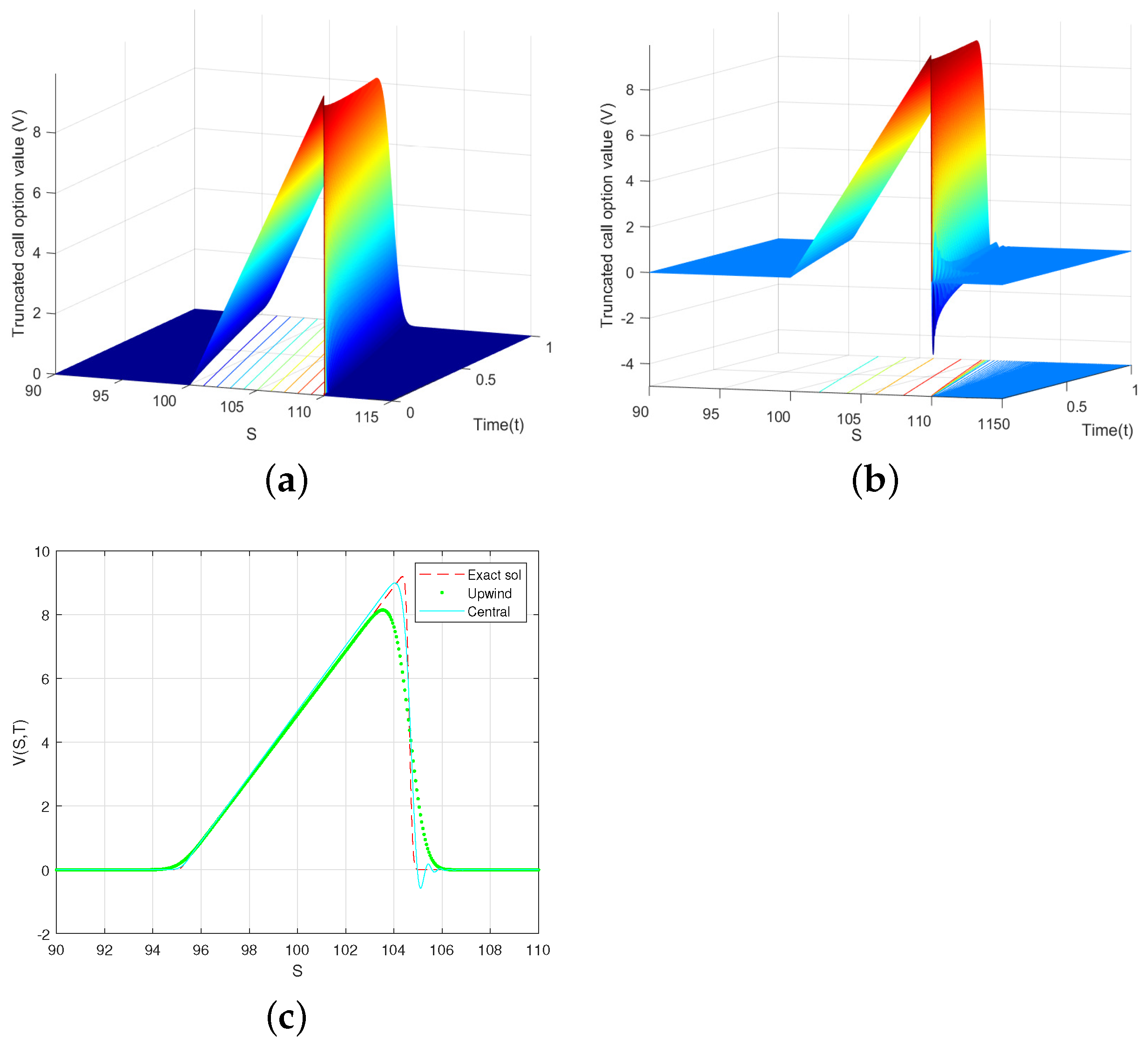
According to Figure 1a, Figure 2a and Figure 3a, the mixed method by using discretization (18) is free of spurious oscillations, and it preserves positivity. The mixed method by using discretization (19) often produces spurious oscillations and negative values in the solution when $\sigma$ and r are satisfied in ${\sigma }^2\ll r$ (see Figure 1b, Figure 2b and Figure 3b). It is shown clearly in Figure 1c, Figure 2c and Figure 3c, in which the cross section at $t=T$ of the analytical solution and different numerical methods are presented. Additionally, in

Table 1. Numerical solutions for the mixed method using the upwind difference and the central difference for $\frac{d{V}^{(k)}}{dS}$ term.

$\mathit{M}=4000,\mathit{S}\to$		95	96	102	103	104	105
For $N=100$
$t=0.2$	Upwind	$9.4810\times {10}^{-17}$	$4.1760\times {10}^{-12}$	$2.9441$	3.9437	4.9433	5.9429
	Central	$1.4900\times {10}^{-22}$	$2.6009\times {10}^{-16}$	2.9581	3.9625	4.9668	5.9712
$t=0.4$	Upwind	$3.5324\times {10}^{-9}$	$6.1635\times {10}^{-6}$	3.9275	4.9266	5.9258	6.9249
	Central	$8.4533\times {10}^{-13}$	$3.7451\times {10}^{-8}$	3.9659	4.9749	5.9838	6.9928
$t=0.6$	Upwind	$5.0885\times {10}^{-5}$	$6.4924\times {10}^{-3}$	4.9002	5.8989	6.8974	7.8717
	Central	$5.7477\times {10}^{-7}$	$8.6729\times {10}^{-4}$	4.9730	5.9865	7.0001	8.0120
For $N=1000$
$t=0.2$	Upwind	$2.9741\times {10}^{-87}$	$9.2550\times {10}^{-68}$	2.0949	3.0948	4.0948	5.0948
	Central	$3.4051\times {10}^{-112}$	$1.3075\times {10}^{-87}$	2.0958	3.0963	4.0967	5.0971
$t=0.4$	Upwind	$9.5591\times {10}^{-75}$	$1.0311\times {10}^{-56}$	2.1946	3.1946	4.1945	5.1944
	Central	$6.0345\times {10}^{-99}$	$7.9996\times {10}^{-76}$	2.1967	3.1976	4.1985	5.1994
$t=0.6$	Upwind	$9.9419\times {10}^{-66}$	$6.0477\times {10}^{-49}$	2.2943	3.2942	4.2940	5.2939
	Central	$3.3916\times {10}^{-89}$	$2.5116\times {10}^{-67}$	2.2976	3.2990	4.3003	5.3017
For N = 10,000
$t=0.2$	Upwind	$7.6032\times {10}^{-184}$	$4.3603\times {10}^{-145}$	2.0095	3.0095	4.0095	5.0095
	Central	$6.4119\times {10}^{-213}$	$2.2017\times {10}^{-168}$	2.010	3.010	4.010	5.010
$t=0.4$	Upwind	$1.3175\times {10}^{-170}$	$2.6163\times {10}^{-133}$	2.0195	3.0195	4.0195	5.0195
	Central	$1.3446\times {10}^{-199}$	$1.5994\times {10}^{-156}$	2.0197	3.0198	4.0199	5.0199
$t=0.6$	Upwind	$7.3729\times {10}^{-161}$	$8.2404\times {10}^{-125}$	2.0295	3.0295	4.0294	5.0294
	Central	$9.1041\times {10}^{-190}$	$6.0974\times {10}^{-148}$	2.0298	3.0299	4.0300	5.0302

, numerical approximations obtained by applying the mixed method at time levels $t=0.2,0.4,0.6$ and different spatial points are calculated for better comparison. The financial parameters for the numerical solution of Equation (15) are taken from [14]. In the following, the strategy of NSFD discretization to overcome the mentioned drawbacks for discretization (19) is used.

4. NSFD Strategy

In this section, a summary of the NSFDs is given, more details on which one can see in [18,19,20,21,22,23,24]. The initial foundation of NSFD schemes originated from the drawbacks of standard finite-difference schemes. Those numerical methods resting on the unsophisticated finite difference approximations which help solve ODEs and PDEs may fail to work properly. Additionally, properties such as positivity of solution may not be transferred to the numerical solution. Consequently, there is a need to devise and investigate numerical methods to solve this problem. To this end, Mickens introduced NSFD methods in [20]. The proposed methods preserve ordinary properties, such as stability, consistency, and convergence. Additionally, they are designed to maintain the qualitative properties of the exact answer.

The NSFD methods can be recognized in two ways: first, how to approximate the derivatives in the equations, and second, how to approximate nonlinear expressions. The forward Euler method is one of the most widely used methods for approximation of the first-order derivative. In the naive case, derivative $V_x$ is approximated by $\frac{V(x+h)-V\left(x\right)}{h}$, in which h represents the step length. In non-standard methods, $V_x$ is approximated by $\frac{V(x+h)-V\left(x\right)}{\psi \left(h\right)}$ so that $\psi \left(h\right)$ is an increasing continuous function of h and satisfies the following relation:

$$\psi \left(h\right)=h+O\left(h^2\right),0<\psi \left(h\right)<1,h\to 0.$$

(25)

It should be noted that whenever h tends to zero, the first derivative must be obtained

$$\frac{\mathrm{d}V}{\mathrm{d}x}=\underset{h\to 0}{lim}{\displaystyle \frac{V(x+{\psi }_1\left(h\right))-V\left(x\right)}{{\psi }_2\left(h\right)}},$$

(26)

where ${\psi }_1\left(h\right)$ and ${\psi }_2\left(h\right)$ are continuous functions of h and satisfy the relation (25). If the numerical method is verified in one of the following conditions, the method is called non-standard:

• In the discretization of the derivatives in the equation using standard finite difference methods, instead of h in the denominator, a complex function such as $\psi$ of h is used which satisfies (26). Therefore, a complex analytic function can be presented that satisfies the following relation:

  $$\psi \left(h\right)=h+O\left(h^2\right),0<\psi \left(h\right)<1,h\to 0,$$

  (27)
  Several functions $\psi \left(h\right)$ that satisfy in (27) are [20]:

  $$h,sin\left(h\right)\mathrm{or}{\displaystyle \frac{1-e^{-\lambda h}}{\lambda }}.$$
• Nonlinear terms in the differential equation are approximated by non-local phrases. The following are instances of this law (see [18,19,20,21,22,23,24]):

  $$\begin{array}{cc}\hfill & V\approx \alpha \left(V_{j+1}+V_{j-1}\right)+\beta \left(V_{j+1}+V_{j-1}\right)+\left(1-2\alpha -2\beta \right)V_j,\alpha ,\beta \in \mathbb{R},\hfill \\ \hfill & V\approx \alpha V_{j-1}+(1-\alpha )V_{j+1},\alpha \in \mathbb{R},\hfill \\ \hfill & V\approx \alpha V_{j-1}+\beta V_{j+1}+(1-\alpha -\beta )V_j,\alpha ,\beta \in \mathbb{R}.\hfill \end{array}$$

It should be noted that there is no general regulation for the selection of the denominator function or non-local approximations. However, there are some general rules in the literature. See for more details [18,19,20,21,22,23,24].

5. The New Scheme

In this section, by using values at different spatial points for discretization $V^{\left(k\right)}$ as

$$\begin{array}{cc}\hfill & V^{\left(k\right)}\approx (\alpha +\beta )\left(V_{j+1}^{\left(k\right)}+V_{j-1}^{\left(k\right)}\right)+\left(1-2\alpha -2\beta \right)V_j^{\left(k\right)},\alpha ,\beta \in \mathbb{R},\hfill \end{array}$$

the new method is proposed:

$$\begin{array}{cc}\hfill & -\frac{1}{2}{\sigma }^2{S}_j^2({\displaystyle \frac{V_{j-1}^{\left(k\right)}-2V_j^{\left(k\right)}+V_{j+1}^{\left(k\right)}}{\Delta S^2}})-r{S}_j({\displaystyle \frac{V_{j+1}^{\left(k\right)}-V_{j-1}^{\left(k\right)}}{2\Delta S}})+(r+\lambda )(\alpha +\beta )\left(V_{j+1}^{\left(k\right)}+V_{j-1}^{\left(k\right)}\right)\hfill \\ \hfill & +(r+\lambda )\left(1-2\alpha -2\beta \right)V_j^{\left(k\right)}=\left\{\begin{array}{cc}v(S,0),\hfill & k=0,\hfill \\ -k{V}^{(k-1)},\hfill & k=1,2,\cdots ,\hfill \end{array}\right.\hfill \end{array}$$

(28)

where $\alpha$ and $\beta$ are the parameters obtained by imposing positivity restrictions. The above discretization may be written in matrix form as follows:

$$\begin{array}{cc}\hfill & \left\{\begin{array}{cc}{\widehat{Q}}_{pw}{V}^{\left(k\right)}=v(S,0),\hfill & k=0,\hfill \\ {\widehat{Q}}_{pw}{V}^{\left(k\right)}=-k{V}^{(k-1)},\hfill & k=1,2,\cdots ,\hfill \end{array}\right.\hfill \end{array}$$

(29)

with

$$\begin{array}{cc}\hfill {\widehat{Q}}_{pw}=& \mathrm{tridiag}\{-\frac{1}{2}{({\displaystyle \frac{\sigma S_j}{\Delta S}})}^2+{\displaystyle \frac{r{S}_j}{2\Delta S}}+(\alpha +\beta )(r+\lambda );{({\displaystyle \frac{\sigma S_j}{\Delta S}})}^2-(2\alpha +2\beta -1)(r+\lambda );\hfill \\ & -\frac{1}{2}{({\displaystyle \frac{\sigma S_j}{\Delta S}})}^2-{\displaystyle \frac{r{S}_j}{2\Delta S}}+(\alpha +\beta )(r+\lambda )\}.\hfill \end{array}$$

The approximation $v_N(S_j,t)$ of $v(S_j,t)$ by using the Post-Widder formula is

$$\begin{array}{c}\hfill v_N(S_j,T)={(\frac{N}{T}{\widehat{Q}}_{PW}^{-1})}^{N+1}v(S_j,0).\end{array}$$

(30)

6. Analysis of the New Scheme

Here, the positivity preservation, stability, consistency and convergence properties of the new method are investigated. Firstly, we present some definitions and results that will be needed in the proof of Theorem 5.

Definition 2.

A matrix $A=\left(a_{ij}\right)$ is called essentially positive if A is irreducible and $a_{ij}\ge 0$, $i\ne j$.

Theorem 3

([25]). A matrix $A\in Z^{n\times n}$ is a nonsingular M-matrix if and only if $A^{-1}$ exists and $A^{-1}\ge 0$.

Definition 3.

A matrix $A=\left(a_{ij}\right)$ is called an L-matrix if $a_{ii}>0$, $\forall i\in N$ and $a_{ij}\le 0$, $i\ne j$.

Theorem 4

([25]). Let A be an L-matrix which is strongly row or column diagonally dominant, i.e., $Ae>0$ or $e^{T}A>0^T$. Then A is a nonsingular M-matrix.

Theorem 5.

Scheme (29) is positive, if

$$\begin{array}{c}\hfill (\alpha +\beta )\le -{\displaystyle \frac{r^2}{8{\sigma }^2(r+\lambda )}}.\end{array}$$

(31)

Proof. 

As the initial condition is positive, if ${\widehat{Q}}_{pw}^{-1}>0$, then we get that scheme (30) is positive. If ${\widehat{Q}}_{pw}$ is an M-matrix, then ${\widehat{Q}}_{pw}^{-1}>0$.

For ${\widehat{Q}}_{pw}$ to be an M-matrix, it should happen that

$$\begin{array}{cc}\hfill & -\frac{1}{2}{({\displaystyle \frac{\sigma S_j}{\Delta S}})}^2+{\displaystyle \frac{r{S}_j}{2\Delta S}}+(\alpha +\beta )(r+\lambda )\le 0,\hfill \\ & \iff (\alpha +\beta )(r+\lambda )\le \frac{1}{2}\left[{({\displaystyle \frac{\sigma S_j}{\Delta S}})}^2-{\displaystyle \frac{r{S}_j}{\Delta S}}\right],\hfill \end{array}$$

(32)

and

$$\begin{array}{cc}\hfill & -\frac{1}{2}{({\displaystyle \frac{\sigma S_j}{\Delta S}})}^2-{\displaystyle \frac{r{S}_j}{2\Delta S}}+(\alpha +\beta )(r+\lambda )\le 0,\hfill \\ \hfill & \iff (\alpha +\beta )(r+\lambda )\le \frac{1}{2}\left[{({\displaystyle \frac{\sigma S_j}{\Delta S}})}^2+{\displaystyle \frac{r{S}_j}{\Delta S}}\right],\hfill \end{array}$$

(33)

and

$$\begin{array}{c}\hfill {({\displaystyle \frac{\sigma S_j}{\Delta S}})}^2-(2\alpha +2\beta -1)(r+\lambda )\ge 0,\Rightarrow (\alpha +\beta )(r+\lambda )\le \frac{1}{2}\left[{({\displaystyle \frac{\sigma S_j}{\Delta S}})}^2+(r+\lambda )\right].\end{array}$$

(34)

From (32)–(34), we can write:

$$\begin{array}{cc}\hfill & (\alpha +\beta )(r+\lambda )\le \frac{1}{2}\left[{({\displaystyle \frac{\sigma S_j}{\Delta S}})}^2-{\displaystyle \frac{r{S}_j}{\Delta S}}\right],\hfill \\ \hfill & ⟺(\alpha +\beta )\le {\displaystyle \frac{1}{2(r+\lambda )}}\left[{({\displaystyle \frac{\sigma S_j}{\Delta S}})}^2-{\displaystyle \frac{r{S}_j}{\Delta S}}\right],\hfill \\ \hfill & ⟺(\alpha +\beta )\le {\displaystyle \frac{{\sigma }^2}{2(r+\lambda )}}\left[{({\displaystyle \frac{S_j}{\Delta S}})}^2-{\displaystyle \frac{r}{{\sigma }^2}}({\displaystyle \frac{S_j}{\Delta S}})+{\displaystyle \frac{r^2}{4{\sigma }^4}}-{\displaystyle \frac{r^2}{4{\sigma }^4}}\right],\hfill \\ \hfill & ⟺(\alpha +\beta )\le {\displaystyle \frac{{\sigma }^2}{2(r+\lambda )}}\left[{\left({\displaystyle \frac{S_j}{\Delta S}}-{\displaystyle \frac{r}{2{\sigma }^2}}\right)}^2-{\displaystyle \frac{r^2}{4{\sigma }^4}}\right],\hfill \\ \hfill & ⟺(\alpha +\beta )\le {\displaystyle \frac{{\sigma }^2}{2(r+\lambda )}}{\left({\displaystyle \frac{S_j}{\Delta S}}-{\displaystyle \frac{r}{2{\sigma }^2}}\right)}^2-{\displaystyle \frac{r^2}{8{\sigma }^2(r+\lambda )}}.\hfill \end{array}$$

(35)

Now, from the last inequality in (35), if $(\alpha +\beta )\le -{\displaystyle \frac{r^2}{8{\sigma }^2(r+\lambda )}}$ then (32) holds. In addition, (33) is a direct consequence of (32). This concludes the proof. □

Theorem 6.

The new method is conditionally stable and convergent to the exact solution with order two with respect to the spatial variable.

Proof. 

According to Theorem 3, ${\widehat{Q}}_{pw}$ is similar to a symmetric tridiagonal matrix (see [25], p. 24) so that the eigenvalues of ${\widehat{Q}}_{pw},{\lambda }_i\left({\widehat{Q}}_{PW}\right),i=1,...,N$ are real.

On the other hand, ${\widehat{Q}}_{pw}$ is row diagonally dominant with

$$\begin{array}{c}\hfill r_i=|a_{ii}|-\sum _{j\ne i}\left|a_{ij}\right|=r+\lambda ,i=1,\dots ,N-1,\end{array}$$

which yields $\parallel {\widehat{Q}}_{pw}^{-1}{\parallel }_{\infty }\le max\frac{1}{r_i}$ (see [25], proposition 1.3). So

$$\begin{array}{c}\hfill \rho ({\widehat{Q}}_{PW}^{-1})\le {\parallel {\widehat{Q}}_{pw}^{-1}\parallel }_{\infty }\le \frac{1}{r+\lambda }=\frac{1}{r+\frac{N}{T}}<1,\end{array}$$

(36)

where $\rho ({\widehat{Q}}_{PW}^{-1})$ is the spectral radius of the matrix ${\widehat{Q}}_{PW}^{-1}$. According to Lex’s theorem [26], the method is stable and convergent, and the local truncation error is equal to

$$\begin{array}{cc}\hfill T_j=& -\frac{1}{2}{\sigma }^2{S}_j^2\left({\displaystyle \frac{V^{(k)}(S_{j-1})-2V^{(k)}(S_j)+V^{(k)}S(j+1)}{\Delta S^2}}\right)-r{S}_j\left({\displaystyle \frac{V^{(k)}(S_{j+1})-V^{(k)}(S_{j-1})}{2\Delta S}}\right)\hfill \\ & +(r+\lambda )[\alpha \left(V^{(k)}(S_{j+1})+V^{(k)}(S_{j-1})\right)\hfill \\ & +\beta \left(V^{(k)}(S_{j+1})+V^{(k)}(S_{j-1})\right)+\left(1-2\alpha -2\beta \right)V^{(k)}(S_j)],\hfill \end{array}$$

(37)

Taylor’s expansion of $V^{(k)}(S_{j-1})$ and $V^{(k)}(S_{j+1})$ around $S_j$ for $j=1,2,\cdots ,n$ is equal to

$$\begin{array}{cc}\hfill & V^{(k)}(S_{j-1})=V_j^{(k)}-\Delta S\left(\frac{d{V}^{(k)}}{dS}\right)+\frac{\Delta S^2}{2!}\left(\frac{d^2{V}^{(k)}}{d{S}^2}\right)-\frac{\Delta S^3}{3!}\left(\frac{d^3{V}^{(k)}}{d{S}^3}\right)+\frac{\Delta S^4}{4!}\left(\frac{d^4{V}^{(k)}}{d{S}^4}\right)+\cdots ,\hfill \\ & V^{(k)}(S_{j+1})=V_j^{(k)}+\Delta S\left(\frac{d{V}^{(k)}}{dS}\right)+\frac{\Delta S^2}{2!}\left(\frac{d^2{V}^{(k)}}{d{S}^2}\right)+\frac{\Delta S^3}{3!}\left(\frac{d^3{V}^{(k)}}{d{S}^3}\right)+\frac{\Delta S^4}{4!}\left(\frac{d^4{V}^{(k)}}{d{S}^4}\right)+\cdots ,\hfill \end{array}$$

by substitution into (37) can write

$$\begin{array}{cc}\hfill T_j=(-\frac{1}{2}{\sigma }^2{S}_j^2\frac{d^2{V}^{(k)}}{d{S}^2}-r{S}_j\frac{d{V}^{(k)}}{dS}+& (r+\lambda )V^{(k)})+(\alpha +\beta )(r+\lambda ){(\Delta S)}^2\left(\frac{d^2{V}^{(k)}}{d{S}^2}\right)\hfill \\ & -\frac{r{S}_j}{3!}{(\Delta S)}^2\left(\frac{d^3{V}^{(k)}}{d{S}^3}\right)+\cdots ,\hfill \end{array}$$

but V is the solution of the ODE, then

$$\begin{array}{c}\hfill \left(-\frac{1}{2}{\sigma }^2{S}_j^2\frac{d^2{V}^{(k)}}{d{S}^2}-r{S}_j\frac{d{V}^{(k)}}{dS}+(r+\lambda )V^{(k)}\right)=0.\end{array}$$

Then, the principal term of the local truncation error (28) is equal to

$$\begin{array}{c}\hfill (\alpha +\beta )(r+\lambda ){(\Delta S)}^2\left(\frac{d^2{V}^{(k)}}{d{S}^2}\right)-\frac{r{S}_j}{3!}{(\Delta S)}^2\left(\frac{d^3{V}^{(k)}}{d{S}^3}\right)+\cdots ,\end{array}$$

which completes the proof. □

7. Numerical Experiments

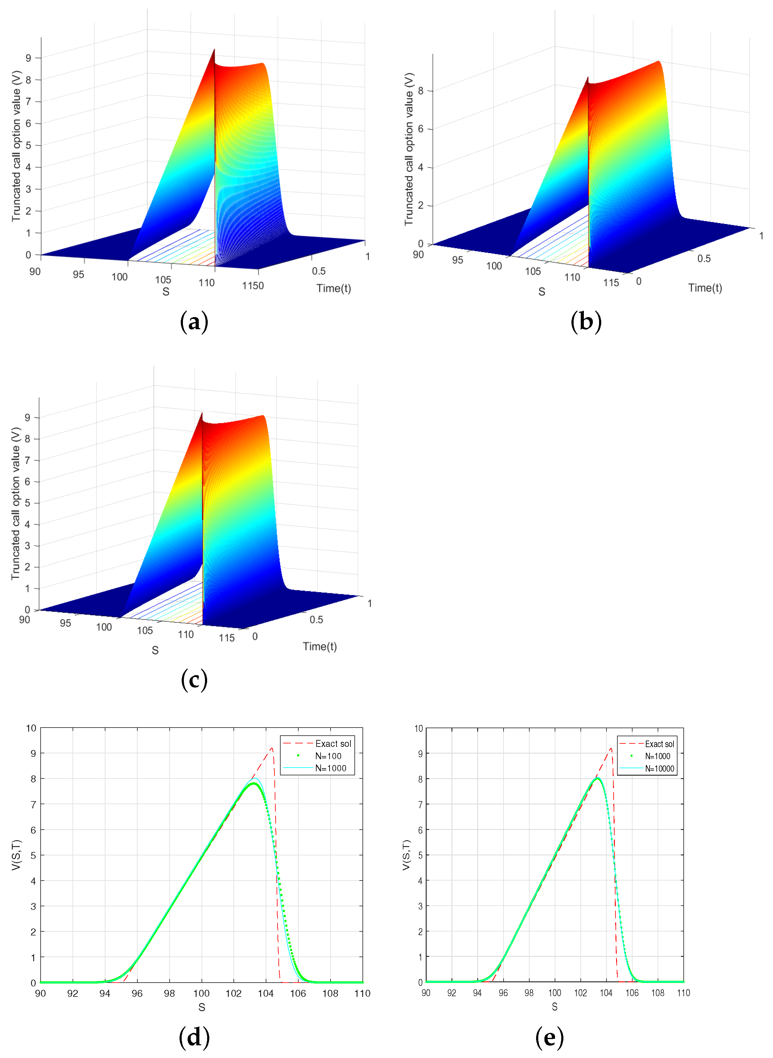
To prove the upside of the newly designed positive scheme with ${\sigma }^2\ll r$, again (17) is considered. In the proposed nonstandard scheme for different N, the solution is acceptable, free of spurious oscillations, and positivity is preserved (see Figure 4a–c). The cross sections of the analytical and numerical solutions at $t=T$ are shown in Figure 4d,e, respectively, using NSFD schemes.

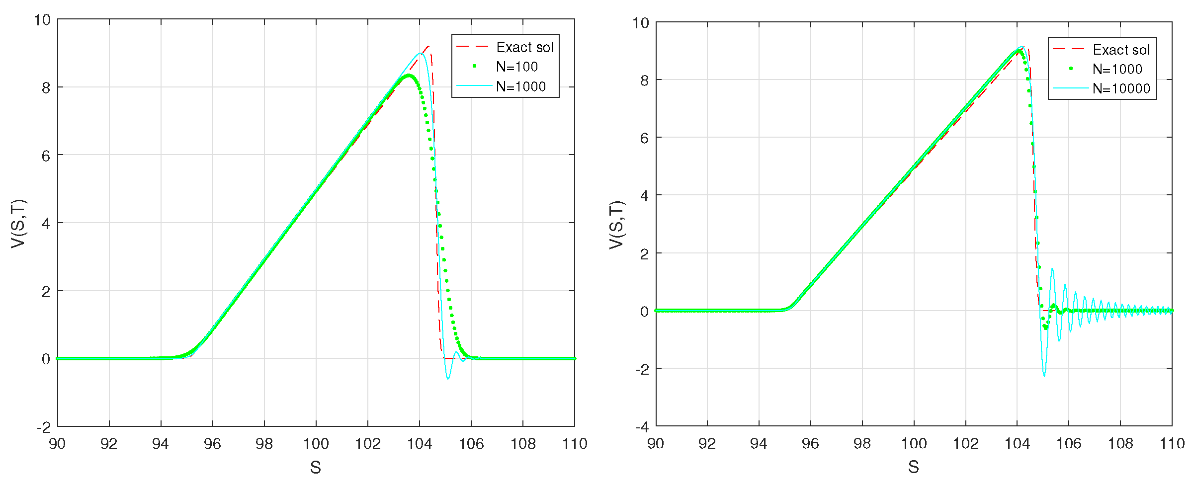
If condition (31) is violated, the solution obtained from the new method may produce abnormal oscillations and negative values in the results (see Figure 5).

The findings suggest that the combination of Laplace transforms method and the standard finite difference method to solve the Black–Scholes equation will lead to numerical issues, including spurious oscillations and numerical diffusion. These issues will rise if ${\sigma }^2\ll r$ and the central differences are employed to discretize the first- and second-order derivatives. Yet, if the Laplace transform method and the NSFD method are used together, we may have smoother behavior of the numerical solution than when the standard finite difference method is used.

Under uncertain economic conditions, sensitivity analysis is one of the best methods to assess investment risk. Indicators such as the time left until expiration of the option, the strike price, the volatility of the underlying asset, and, last but not least, the interest rate, are all important when determining the price of the options. Now, we will briefly review these variables and the consequences, viz, the calculation of sensitivities or Greeks, the most significant of which are

$$\begin{array}{cc}\hfill & \mathrm{Delta}\Delta ={\displaystyle \frac{\partial V}{\partial S}},\hfill \\ \hfill & \mathrm{Gamma}\Gamma ={\displaystyle \frac{{\partial }^{2}V}{\partial S^2}}.\hfill \end{array}$$

Delta represents the change in the price of an option as a result of the stock prices falling or rising. If the price sensitivity of the option to stock price is determined, the buyer can determine the amount of loss or gain incurred if the option contract is not exercised, as well as the maximum loss that may incur if the contract is not exercised.

The ratio of the change in Delta to the change in stock prices is called Gamma. The extent to which portfolio composition needs to change and be adapted can be determined by investors and buyers based on this parameter. The latter is comprised of shares and stock options, which help maintain a trading position during these changes. The portfolio’s structure and size will be less likely to fluctuate if the Gamma value is low. On the contrary, if the Gamma value increases, the need for such variation will be increased.

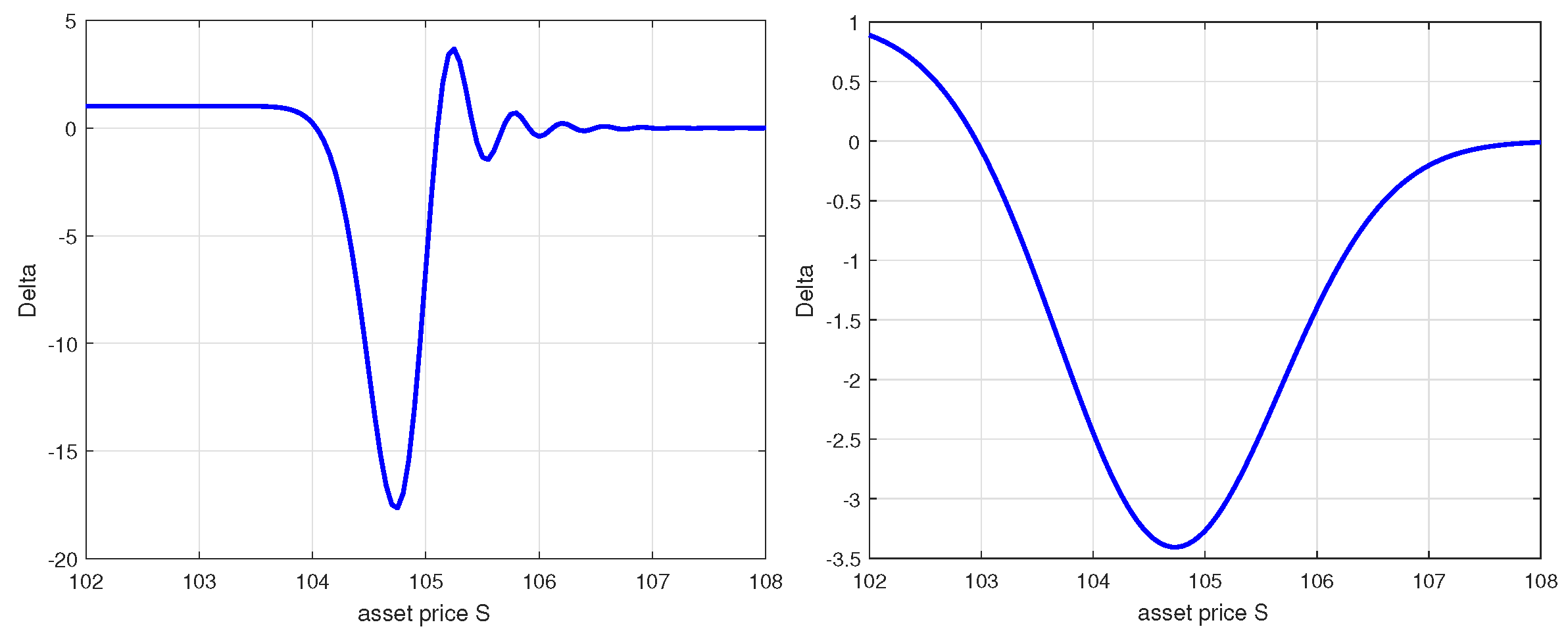
Now, using the mixed and NSFD schemes, Delta and Gamma are compared for $N=1000$. Figure 6 presents the results for Delta. The value of Delta using the mixed scheme generates spurious oscillations, while using the NSFD scheme cause the elimination of these oscillations. Furthermore, Figure 7 depicts the results for Gamma. The value of Gamma in the mixed scheme generates spurious oscillations, while applying the NSFD scheme eliminates these oscillations.

8. Conclusions and Discussion

In this article, one new NSFD scheme to numerically solve the BSM model is applied, which is used for options pricing. This scheme is derived by combining the Laplace transform method and the NSFD strategy. The results show that the new method retains the essential qualitative properties, such as positivity and stability. The local truncation error of the new scheme is $\mathcal{O}(\Delta S^2)$. The results of the novel method compared with those of other standard numerical methods, such as the mixed method, indicate that the unmistaken implementation of the method we have devised produces numerical solutions for the Black–Scholes equation. The results suggest that non-standard difference schemes may be of use when solving problems that can exert influence on the stock price similar to nonlinear Black–Scholes equations and generalized BSM models. The proposed method can be extended to a high-order method and for a class of nonlinear Black–Scholes equation [27].

References

1. Black, F.; Scholes, M. The pricing of options and corporate liabilities. J. Political Econ. 1973, 81, 637–659. [Google Scholar] [CrossRef]
2. Hout, K.J.; Volders, K. Stability of central finite difference schemes on non-uniform grids for the Black–Scholes equation. Appl. Numer. Math. 2009, 59, 2593–2609. [Google Scholar] [CrossRef]
3. Milev, M.; Tagliani, A. Numerical valuation of discrete double barrier options. J. Comput. Appl. Math. 2010, 233, 2468–2480. [Google Scholar] [CrossRef]
4. Pealat, G.; Duffy, D.J. The alternating direction explicit (ADE) method for one-factor problems. Wilmott 2011, 2011, 54–60. [Google Scholar] [CrossRef]
5. Golbabai, A.; Ballestra, L.V.; Ahmadian, D. Superconvergence of the finite element solutions of the Black–Scholes equation. Financ. Res. Lett. 2013, 10, 17–26. [Google Scholar] [CrossRef]
6. Mehdizadeh Khalsaraei, M.; Shokri Jahandizi, R. A modified explicit method for the Black–Scholes equation with positivity preserving property. J. Math. Comput. Sci. 2015, 15, 299–305. [Google Scholar] [CrossRef]
7. Farnoosh, R.; Sobhani, A.; Beheshti, M.H. Efficient and fast numerical method for pricing discrete double barrier option by projection method. Comput. Math. Appl. 2017, 73, 1539–1545. [Google Scholar] [CrossRef]
8. Jeong, D.; Yoo, M.; Kim, J. Finite difference method for the Black–Scholes equation without boundary conditions. Comput. Econ. 2018, 51, 961–972. [Google Scholar] [CrossRef]
9. Heo, Y.; Han, H.; Jang, H.; Chot, Y.; Kim, J. Finite difference method for the two-dimensional Black–Scholes equation whit a hybrid boundary condition. J. Korean Soc. Ind. Appl. Math. 2019, 23, 19–30. [Google Scholar]
10. Abdi-Mazraeh, S.; Khani, A.; Irandoust-Pakchin, S. Multiple shooting method for solving Black–Scholes equation. Comput. Econ. 2020, 56, 723–746. [Google Scholar] [CrossRef]
11. Shokri, A.; Saadat, H. Trigonometrically fitted high-order predictor-corrector method with phase-lag of order infinity for the numerical solution of radial Schrödinger equation. J. Math. Chem. 2014, 52, 1870–1894. [Google Scholar] [CrossRef]
12. Shokri, A. The symmetric two-step P-stable nonlinear predictor-corrector methods for the numerical solution of second order initial value problems. Bull. Iran. Math. Soci. 2015, 41, 201–215. [Google Scholar]
13. Roul, P.; Goura, V.M.K. A sixth order numerical method and its convergence for generalized Black–Scholes PDE. J. Comput. Appl. Math. 2020, 377, 112881. [Google Scholar] [CrossRef]
14. Milev, M.; Tagliani, A. Laplace transform and finite difference methods for the Black–Scholes equation. Appl. Math. Comput. 2013, 220, 649–658. [Google Scholar]
15. Cohen, A.M. Numerical Methods for Laplace Transform Inversion; Springer: New York, NY, USA, 2007. [Google Scholar]
16. Schiff, J.L. The Laplace Transform, Theory and Applications; Springer: New York, NY, USA, 1999. [Google Scholar]
17. Duffy, D.G. Transform Methods for Solving Partial Differential Equations; Chapman and Hall/CRC: Boca Raton, FL, USA, 2004. [Google Scholar]
18. Mehdizadeh Khalsaraei, M.; Shokri, A.; Ramos, H.; Heydari, S. A positive and elementary stable nonstandard explicit scheme for a mathematical model of the influenza disease. Math. Comput. Simul. 2021, 182, 397–410. [Google Scholar] [CrossRef]
19. Merton, R.C. Theory of rational option pricing. Bell J. Econ. Manag. Sci. 1973, 4, 141–183. [Google Scholar] [CrossRef]
20. Mickens, R.E. Nonstandard Finite Difference Models of Differential Equations; World Scientific: Singapore, 1994. [Google Scholar]
21. Mickens, R.E.; Jordan, P.M. A positivity-preserving nonstandard finite difference scheme for the damped wave equation. Numer. Meth. Par. Differ. Equ. 2004, 20, 639–649. [Google Scholar] [CrossRef]
22. Mickens, R.E.; Jordan, P.M. A new positivity-preserving nonstandard finite difference scheme for the DWE. Numer. Meth. Par. Differ. Equ. 2005, 21, 976–985. [Google Scholar] [CrossRef]
23. Milev, M.; Tagliani, A. Efficient implicit scheme with positivity preserving and smoothing properties. J. Comput. Appl. Math. 2013, 243, 1–9. [Google Scholar] [CrossRef]
24. Milev, M.; Tagliani, A. Low volatility options and numerical diffusion of finite difference schemes. Serd. Math. J. 2010, 36, 223–236. [Google Scholar]
25. Windish, G. M-matrices in numerical analysis. In Teubner-Texte Zur Mathematik; Vieweg+Teubner Verlag: Leipzig, Germany, 1989; Volume 115. [Google Scholar]
26. Smith, G.D. Numerical Solution of Partial Differential Equation: Finite Difference Method; Clarendon Press: Oxford, UK, 1985. [Google Scholar]
27. Jha, N.; Wagley, M. Stability Analysis of Quasi-variable Grids Cubic Spline Fourth-Order Compact Implicit Algorithms for Burger’s Type Parabolic PDEs. Iran. J. Sci. Technol. Trans. A 2020, 44, 1875–1890. [Google Scholar] [CrossRef]
Figure 1. Call option value for r = 0.05 , σ = 0.001 , T = 1 , U = 110 , K = 100 , L = 90 , S max = 200 , Δ S = 0.05 , N = 100 . (a) The mixed method using discretization (18). (b) The mixed method using discretization (19). (c) Solutions at t = T .
Fractalfract 07 00154 g001
Figure 2. Call option value for r = 0.05 , σ = 0.001 , T = 1 , U = 110 , K = 100 , L = 90 , S max = 200 , Δ S = 0.05 , N = 1000 . (a) The mixed method using discretization (18). (b) The mixed method using discretization (19). (c) Solutions at t = T .
Fractalfract 07 00154 g002
Figure 3. Call option value for r = 0.05 , σ = 0.001 , T = 1 , U = 110 , K = 100 , L = 90 , S max = 200 , Δ S = 0.05 , N = 10,000. (a) The mixed method using discretization (18). (b) The mixed method using discretization (19). (c) Solutions at t = T .
Fractalfract 07 00154 g003
Figure 4. Call option value for r = 0.05 , σ = 0.001 , T = 1 , U = 110 , K = 100 , L = 90 , S max = 200 , Δ S = 0.05 . (a) The NSFD method with N = 100 . (b) The NSFD method with N = 1000 . (c) The NSFD method with N = 10,000. (d) Compare solutions for N = 100 and N = 1000 at t = T . (e) Compare solutions for N = 1000 and N = 10,000 at t = T .
Fractalfract 07 00154 g004
Figure 5. Condition (31) is violated. Call option value for r = 0.05 , σ = 0.001 , T = 1 , U = 110 , K = 100 , L = 90 , S max = 200 , Δ S = 0.05 .
Fractalfract 07 00154 g005
Figure 6. Delta using the mixed scheme (left) and the NSFD scheme (right), with finance data r = 0.05 , σ = 0.001 , K = 100 , T = 1 , U = 110 , L = 90 , S m a x = 200 , Δ S = 0.05 and Δ t = 10 3 .
Fractalfract 07 00154 g006
Figure 7. Gamma using the mixed scheme (left) and the NSFD scheme (right), with finance data r = 0.05 , σ = 0.001 , K = 100 , T = 1 , U = 110 , L = 90 , S m a x = 200 , Δ S = 0.05 and Δ t = 10 3 .
Fractalfract 07 00154 g007