On Constructing a Family of Sixth-Order Methods for Multiple Roots

Abstract

A family of three-point, sixth-order, multiple-zero solvers is developed, and special cases of weight functions are investigated based on polynomials and low-order rational functions. The chosen cases of the proposed iterative method are compared with existing methods. The experiments show the superiority of the proposed schemes in terms of the number of divergent points and the average number of function evaluations per point. The dynamical characteristics of the developed methods, along with their illustrations, are represented with detailed analyses, comparisons, and comments.

1. Introduction

Nonlinear equations [1,2,3,4] occur frequently in various fields of science, artificial intelligence, and engineering. Finding the roots of a nonlinear equation [5,6,7,8] involves determining the value of a variable that satisfies a given equation. A zero $\alpha$ of $h\left(x\right)=0$ is called a multiple root with multiplicity m if $h^{\left(i\right)}\left(\alpha \right)=0,i=0,1,2,\cdots ,m-1$ and $h^{\left(m\right)}\left(\alpha \right)\ne 0$.

It is known that the Newton method is the most used method for solving the equations, given by

$$x_{n+1}=x_n-m\frac{f\left(x_n\right)}{f^{\prime }\left(x_n\right)},n=0,1,2,\cdots .$$

(1)

Researchers [9,10,11,12,13,14,15] are interested in finding multiple roots of nonlinear equations [16,17,18,19,20] and investigating the dynamics by exploring the relevant basins of attraction [21,22,23,24,25,26].

Geum-Kim-Neta [27,28] constructed a class of two-point, sixth-order, multiple-root solvers. Since the following two methods are faster and require fewer iterations per point on average, we have chosen two methods as follows. These two schemes, called here (X1) and (X2), are given by

$$\left\{\begin{array}{c}{y}_n=x_n-m\frac{f\left(x\right)}{f^{\prime }\left(x\right)},\hfill \\ x_{n+1}=y_n-m[2(m-1)(u-s)-u^2-2us+1]h,\hfill \end{array}\right.$$

(2)

and

$$\left\{\begin{array}{c}{y}_n=x_n-m\frac{f\left(x_n\right)}{f^{\prime }\left(x_n\right)},\hfill \\ x_{n+1}=y_n-\frac{au+m}{+c{u}^2+1+b\ast u}·\frac{1}{1+ds},\hfill \end{array}\right.$$

(3)

where

$$\begin{array}{cc}\hfill a=& \frac{13+2m(4m^4-16m^3+31m^2-30m+13)}{(m-1)(7+4m^2-8m)},b=\frac{4(2m^2-4m+3)}{(m-1)(4m^2-8m+7)},\hfill \\ \hfill c=& -\frac{3+4m^2-8m}{7+4m^2-8m},d=2(m-1),u={\left(\frac{f\left(y_n\right)}{f\left(x_n\right)}\right)}^{\frac{1}{m}},\hfill \\ \hfill s=& {\left(\frac{f^{\prime }\left(y_n\right)}{f^{\prime }\left(x_n\right)}\right)}^{\frac{1}{m-1}}.\hfill \end{array}$$

In this paper, we propose a three-point, sixth-order method by adding a third step, as follows:

$$\left\{\begin{array}{c}{y}_n=x_n-m\frac{f\left(x_n\right)}{f^{\prime }\left(x_n\right)},\hfill \\ w_n=x_n-m{A}_f\left(k\right)\frac{f\left(x_n\right)}{f^{\prime }\left(x_n\right)},k={\left(\frac{f^{\prime }\left(y_n\right)}{f^{\prime }\left(x_n\right)}\right)}^{\frac{1}{m-1}},\hfill \\ x_n=x_n-m{B}_f(k,v)\frac{f\left(x_n\right)}{f^{\prime }\left(x_n\right)},v={\left(\frac{f\left(w_n\right)}{f\left(x_n\right)}\right)}^{\frac{1}{m}},\hfill \end{array}\right.$$

(4)

where $A_f:C\to C$ is analytic in a small neighborhood of 0, and $B_f:C^2\to C$ is holomorphic in a neighborhood of $(0,0)$.

Definition 1.

Let $a_0,a_1,\cdots a_n\cdots$ be a sequence converging to a zero α and $e_n=a_n-\alpha$ be the n-th iterative error. If there exist real numbers $\beta \in R$ and $\delta \in R-\left\{0\right\}$, such that the following error equations satisfy

$$e_{n+1}=\delta {e_n}^{\beta }+O\left({e_n}^{\beta +1}\right),$$

then $\left|\delta \right|$ or δ is called the asymptotic error constant, and β is defined as the order of convergence [1].

Definition 2.

Suppose that the theoretical asymptotic error constant $\omega ={lim}_{n\to \infty }\frac{|e_n|}{|e_{n-1}{|}^{\beta }}$ and the convergence order $\beta \ge 1$ are known [2,3]. The computational convergence order ${\beta }_n=\frac{log|e_n/\omega |}{log|e_{n-1}|}$ is defined. Then ${lim}_{n\to \infty }{\beta }_n=\beta$.

Definition 3.

If a fixed point ρ of a rational map J is attracting, then all nearby points of ρ are attracted to ρ under a rational map J. The collection of all points whose iterates under J converge to ρ is called the basin of attraction of ρ.

We investigate the convergence behavior of the proposed scheme in Section 2. The numerical results and the basins of attraction for the typical examples are shown in Section 3. In addition, the basins of attraction for the equation in the blood rheology model are shown, and the convergent regions for selected values are plotted in Section 3. Finally, Section 4 is discussed in the last section.

2. Convergence Analysis

In this section, we determine the maximal convergence order of the developed schemes. We investigate the main theorem describing the convergent behavior of the proposed schemes and address how to construct weight functions $A_f$ and $B_f$ for sixth-order convergence. It is sufficient to consider weight functions $A_f$ and $B_f$ up to the fifth-order terms in $e_n$ in terms of $O\left(\frac{f\left(x_n\right)}{f^{\prime }\left(x_n\right)}\right)=O\left(e_n\right)$.

Let a function $f:C\to C$ have a root $\alpha$ of multiplicity $m>1$ and be analytic in a small neighborhood of $\alpha$.

$$\begin{array}{cc}\hfill y_n=& x_n-m\frac{f\left(x_n\right)}{f^{\prime }\left(x_n\right)},\hfill \\ \hfill w_n=& x_n-m·A_f\left(k\right)·\frac{f\left(x_n\right)}{f^{\prime }\left(x_n\right)},k={\left(\frac{f^{\prime }\left(y_n\right)}{f^{\prime }\left(x_n\right)}\right)}^{\frac{1}{m-1}},\hfill \\ \hfill x_n=& x_n-m·B_f(k,v)·\frac{f\left(x_n\right)}{f^{\prime }\left(x_n\right)},v={\left(\frac{f\left(w_n\right)}{f\left(x_n\right)}\right)}^{\frac{1}{m}},\hfill \end{array}$$

where $A_f:C\to C$ is analytic in a small neighborhood of the origin 0 and $B_f:C^2\to C$ is holomorphic in a small neighborhood of $(0,0)$.

Using the Taylor expansion about $\alpha$, we have

$$f\left(x_n\right)=e^m\Gamma (1+{\theta }_2{e}_n+{\theta }_3{e_n}^2+{\theta }_4{e_n}^3+{\theta }_5{e_n}^4+{\theta }_6{e_n}^5+{\theta }_7{e_n}^6+O\left({e_n}^7\right)),$$

(5)

$$\begin{array}{cc}\hfill f^{\prime }\left(x_n\right)=& e^{m-1}\Gamma (m+(1+m){\theta }_2{e}_n+(2+m){\theta }_3{e_n}^2+(3+m){\theta }_4{e_n}^3+(4+m){\theta }_5{e_n}^4\hfill \\ \hfill & +(5+m){\theta }_6{e_n}^5+(6+m){\theta }_7{e_n}^6+O\left({e_n}^7\right)),\hfill \end{array}$$

(6)

where $\Gamma =\frac{f^{\left(m\right)}\left(\alpha \right)}{m!}$, ${\theta }_j=\frac{m!}{(m+j-1)!}\frac{f^{(m+j-1)}\left(\alpha \right)}{f^{\left(m\right)}\left(\alpha \right)}$ for $j\in N-\left\{1\right\}$.

For convenience, we denote $e_n$ by e without subscript n. Dividing (5) by (6), we have

$$\frac{f\left(x_n\right)}{f^{\prime }\left(x_n\right)}=\frac{e}{m}-\frac{{\theta }_2{e}^2}{m^2}+\frac{t_3{e}^3}{m^3}+\frac{t_4{e}^4}{m^4}+\frac{t_5{e}^5}{m^5}+\frac{t_6{e}^6}{m^6}+O\left(e^7\right),$$

(7)

where

$$\begin{array}{cc}\hfill t_3=& ((1+m){{\theta }_2}^2-2m{\theta }_3),\hfill \\ \hfill t_4=& (-{(1+m)}^2{{\theta }_2}^3+m(4+3m){\theta }_2{\theta }_3-3m^2{\theta }_4),\hfill \\ \hfill t_5=& {(1+m)}^3{{\theta }_2}^4-2m(3+5m+2m^2){{\theta }_2}^2{\theta }_3+2m^2(3+2m){\theta }_2{\theta }_4\hfill \\ \hfill & +2m^2((2+m){{\theta }_3}^2-2m{\theta }_5),\hfill \end{array}$$

and

$$\begin{array}{cc}\hfill t_6=& -{(1+m)}^4{{\theta }_2}^5+m{(1+m)}^2(8+5m){{\theta }_2}^3{\theta }_3-m^2(9+14m+5m^2){{\theta }_2}^2{\theta }_4\hfill \\ \hfill & +m^2{\theta }_2(-\left((12+16m+5m^2){{\theta }_3}^2\right)+m(8+5m){\theta }_5)+m^3((12+5m){\theta }_3{\theta }_4-5m{\theta }_6).\hfill \end{array}$$

By Taylor’s expansion, we have expression k, as follows:

$$\begin{array}{cc}\hfill k=& {\left(\frac{f^{\prime }\left(y_n\right)}{f^{\prime }\left(x_n\right)}\right)}^{\frac{1}{m-1}},=\frac{{\theta }_2}{m}e+\frac{-m(1+m){{\theta }_2}^2-2m(1-m){\theta }_3}{m(-1+m)}{e}^2\hfill \\ \hfill & +\frac{w_3}{2{(m-1)}^2}{e}^3+\frac{w_4}{6{(-1+m)}^3}{e}^4+\frac{w_5}{24{(-1+m)}^4}{e}^5+\frac{w_6}{120{(-1+m)}^5}{e}^6+O\left(e^7\right)),\hfill \end{array}$$

(8)

where $w_i=w_i({\theta }_2,{\theta }_3,\cdots {\theta }_6)$ for $3\le i\le 6$.

Using k in (8), and expanding the Taylor series of $A_f\left(k\right)$ about 0 up to the fifth-order term, we find

$$A_f\left(k\right)=A_0+A_{1}k+A_2{k}^2+A_3{k}^3+A_4{k}^4+A_5{k}^5+O\left(e^6\right),$$

(9)

where $A_j=\frac{{A_f}^{\left(j\right)}\left(0\right)}{j!}$ for $0\le j\le 5$.

Substituting (5)–(9) into $w_n$, we have

$$w_n=\alpha +(1-A_0)e+\frac{(A_0-A_1)}{m}{\theta }_2{e}^2+z_3{e}^3+z_4{e}^4+z_5{e}^5+z_6{e}^6+O\left(e^7\right),$$

(10)

where

$z_3=\frac{(A_0-A_1+A_2+2A_{1}m-A_{2}m-A_0{m}^2+A_1{m}^2){{\theta }_2}^2+(-2A_{0}m+2A_{1}m+2A_0{m}^2-2A_2{m}^2){\theta }_3}{m^2(-1+m)},$

$z_i=z_i({\theta }_2,\cdots {\theta }_n,A_0,A_1,\cdots A_4)$ for $4\le i\le 6$.

Choosing $A_0=A_1=1$, $A_2=\frac{2m}{-1+m}$, we have

$$\begin{array}{cc}\hfill w_n=& \alpha +\frac{((2+m+m^3-2m^2(-4+A_3)-2A_3+4m{A}_3){{\theta }_2}^3-2(-1+m)m^2{\theta }_2{\theta }_3)}{2m^3{(-1+m)}^2}{e}^4\hfill \\ \hfill & +z_5{e}^5+z_6{e}^6+O\left(e^7\right).\hfill \end{array}$$

(11)

Then we obtain

$$\begin{array}{cc}\hfill f\left(w_n\right)=& \frac{e^{4m}\Gamma }{(-1+m)3^m}({\frac{1}{2}(2+m+m^3-2m^2(-4+A_3)-2A_3+4m{A}_3){{\theta }_2}^3-(-1+m)m^2{\theta }_2{\theta }_3}^m\hfill \\ \hfill & +\frac{1}{3}{((2+m+m^3-2m^2(-4+A_3)-2A_3+4m{A}_3){{\theta }_2}^3-2(-1+m)m^2{\theta }_2{\theta }_3)}^{-1+m}\hfill \\ \hfill & \left(\right(-7m^5+2m^4(-35+9A_3)+m(17+36A_3-18A_4)\hfill \\ \hfill & +6(2-A_3+A_4)-6m^3(9+2A_3+A_4)+m^2(14-36A_3+18A_4)){{\theta }_2}^4\hfill \\ \hfill & +12(-1+m)m(2+m+2m^3-3m^2(-4+A_3)-3A_3+6m{A}_3){{\theta }_2}^2{\theta }_3\hfill \\ \hfill & -12{(-1+m)}^2{m}^3{{\theta }_3}^2-12{(-1+m)}^2{m}^3{\theta }_2{\theta }_4)e+w_2{e}^2+w_3{e}^3+O\left(e^4\right)),\hfill \end{array}$$

(12)

where $w_i=w_i({\theta }_2,\cdots {\theta }_n,A_3,A_4),i=2,3$.

With the use of (5) and (12), we have v as follows:

$$\begin{array}{cc}\hfill v=& \frac{((2+m+m^3-2m^2(-4+A_3)-2A_3+4m{A}_3){{\theta }_2}^3-2(-1+m)m^2{\theta }_2{\theta }_3}{2{(-1+m)}^2{m}^3}{e}^3\hfill \\ \hfill & +\frac{1}{6{(-1+m)}^3{m}^4}\left(\right(-7m^5+m^4(-73+18A_3)+2m(7+27A_3-9A_4)\hfill \\ \hfill & +6(3-2A_3+A_4)-3m^3(25+2A_3+2A_4)+m^2(35-54A_3+18A_4)){{\theta }_2}^4\hfill \\ \hfill & +6(-1+m)m(4+m+4m^3+m^2(25-6A_3)-6A_3+12m{A}_3){{\theta }_2}^2{\theta }_3\hfill \\ \hfill & -12{(-1+m)}^2{m}^3{{\theta }_3}^2-12{(-1+m)}^2{m}^3{\theta }_2{\theta }_4)e^4+v_5{e}^5+O\left(e^6\right),\hfill \end{array}$$

(13)

where $v_5=v_5({\theta }_2,\cdots {\theta }_n,A_1,\cdots A_4)$.

Expanding the Taylor series of $B_f(k,v)$ about (0,0) up to the fifth-order term, we find

$$B_f(k,v)=B_{00}+B_{30}{k}^3+B_{40}{k}^4+B_{50}{k}^5+B_{01}v+k(B_{10}+B_{11}v)+k^2(B_{20}+B_{21}v)+O\left(e^6\right),$$

(14)

where $B_{ij}=\frac{1}{i!j!}\frac{{\partial }^{i+j}}{\partial k^i\partial v^j}{B}_f{(k,v)|}_{(k=0,v=0)}$ for $0\le i\le 5,0\le j\le 1$.

By Substituting (5)–(14) into the proposed scheme (4), we have

$$\begin{array}{cc}\hfill & x_{n+1}-\alpha =x_n-\alpha -B_f(k,v)\frac{f\left(x_n\right)}{f^{\prime }\left(x_n\right)}\hfill \end{array}$$

(15)

$$\begin{array}{cc}\hfill & =C_{1}e+C_2{e}^2+C_3{e}^3+C_4{e}^4+C_5{e}^5+C_6{e}^6+O\left(e^7\right),\hfill \end{array}$$

(16)

where $C_1=1-B_{00}$ and the coefficients $C_i(2\le i\le 6)$ depend of m, $A_j(j=0,1,\cdots 5)$, and ${\theta }_i(i=1,2,\cdots )$.

Solving $C_1$ for $B_{00}$, we have

$$B_{00}=1.$$

(17)

Using $B_{00}=1$ into $C_2$, we have

$$B_{10}=1.$$

(18)

Substituting $B_{00}=B_{10}=1$ into $C_3$, we obtain $\frac{(B_{20}+2m-B_{20}m){{\theta }_2}^2}{m(m-1)}=0$.

From which we find

$$B_{20}=\frac{2m}{-1+m}.$$

(19)

Substituting $B_{00}=B_{10}=1$ and $B_{20}=\frac{2m}{-1+m}$ into $C_4=0$, we have

$$\begin{array}{cc}\hfill C_4=& \frac{1}{2{(-1+m)}^2}{m}^{-\frac{3m}{-1+m}}(2(4+(-4+A_3)B_{01}-B_{30})m^{2+\frac{3}{-1+m}}\hfill \\ \hfill & -2(-1+B_{01}-A_3{B}_{01}+B_{30})m^{\frac{3}{-1+m}}+(1-B_{01})m^{\frac{3m}{-1+m}}\hfill \\ \hfill & +(-1-B_{01}-4A_4{B}_{01}+4B_{30})m^{\frac{2+m}{-1+m}}){{\theta }_2}^3\hfill \\ \hfill & +\frac{m^{-\frac{3m}{-1+m}}(2m^{2+\frac{3}{-1+m}}-2B_{01}{m}^{2+\frac{3}{-1+m}}-2(-1-B_{01})m^{\frac{3m}{-1+m}}){\theta }_2{\theta }_3}{2{(-1+m)}^2}.\hfill \end{array}$$

and

$$B_{01}=1,B_{30}=A_3.$$

(20)

Substituting $B_{00}=B_{10}=1$, $B_{20}=\frac{2m}{-1+m}$$B_{01}=1,B_{30}=A_3$ into $C_5=0$, we have

$$\begin{array}{cc}\hfill C_5=& \frac{1}{2{(-1+m)}^3}{m}^{-\frac{4m}{-1+m}}\left((-14-6A_4-6A_3(-2+B_{11})+7B_{11}+6B_{40})\right)m^{2+\frac{4}{-1+m}}+\hfill \\ \hfill & (14+2A_4+2A_3(-2+B_{11})-7B_{11}-2B_{40})m^{3+\frac{4}{-1+m}}\hfill \\ \hfill & +2(-2-A_4-A_3(-2+B_{11})+B_{11}+B_{40})m^{\frac{4}{-1+m}})\hfill \\ \hfill & +(2-B_{11})m^{\frac{4m}{-1+m}}+(2+6A_4+6A_3(-2+B_{11})-B_{11}-6B_{40})m^{\frac{3+m}{-1+m}}{{\theta }_2}^4\hfill \\ \hfill & +\frac{m^{-\frac{4m}{-1+m}}(2(-2+B_{11})m^{2+\frac{4}{-1+m}}-4(-2+B_{11})m^{3+\frac{4}{-1+m}}-2(2-B_{11})m^{\frac{4m}{-1+m}}){{\theta }_2}^2{\theta }_3}{2{(-1+m)}^3},\hfill \end{array}$$

and

$$B_{40}=A_4,B_{11}=2.$$

(21)

Putting (17)–(21) into $C_6$, we obtain

$$\begin{array}{cc}\hfill C_6=& \frac{p_1{{\theta }_2}^5+p_2{{\theta }_2}^3{\theta }_3+p_3{\theta }_2{{\theta }_3}^2}{4{(-1+m)}^3{m}^5},\hfill \end{array}$$

(22)

where

$$\begin{array}{cc}\hfill p_1=& 4A_5{(-1+m)}^3+4A_3{B}_{21}{(-1+m)}^3-4B_{50}{(-1+m)}^3-2B_{21}(-1+m)\hfill \\ \hfill & (2+m+8m^2+m^3)+(2-2A_3{(-1+m)}^2+m+m^2(8+m))(-3+m(10+m)),\hfill \\ \hfill p_2=& -4(-1+m)m(1+m^3-A_3-m^2(-9+B_{21}+A_3)+m(-1+B_{21}+2A_3)),\hfill \\ \hfill p_3=& 4{(-1+m)}^2{m}^3.\hfill \end{array}$$

Then the proposed method, (4), is of the sixth order and possesses the following error equation:

$$\begin{array}{cc}\hfill e_{n+1}=& \frac{p_1{{\theta }_2}^5+p_2{{\theta }_2}^3{\theta }_3+p_3{\theta }_2{{\theta }_3}^2}{4{(-1+m)}^3{m}^5}{e_n}^6+O\left({e_n}^7\right),\hfill \end{array}$$

(23)

where

$$\begin{array}{cc}\hfill p_1=& 4A_5{(-1+m)}^3+4A_3{B}_{21}{(-1+m)}^3-4B_{50}{(-1+m)}^3-2B_{21}(-1+m)\hfill \\ \hfill & (2+m+8m^2+m^3)+(2-2A_3{(-1+m)}^2+m+m^2(8+m))(-3+m(10+m)),\hfill \\ \hfill p_2=& -4(-1+m)m(1+m^3-A_3-m^2(-9+B_{21}+A_3)+m(-1+B_{21}+2A_3)),\hfill \\ \hfill p_3=& 4{(-1+m)}^2{m}^3.\hfill \end{array}$$

Theorem 1.

Let $m\in N-\left\{1\right\}$. Let a function $f:C\to C$ have a multiple root α with multiplicity m. Assume that f is analytic in a neighborhood of α. Let ${\theta }_j=\frac{m!}{(m+j-1)!}\frac{f^{(n+j-1)}\left(\alpha \right)}{f^{\left(m\right)}\left(\alpha \right)}$ for $j\in N-\left\{1\right\}$. Let $x_0$ be an initial value in a neighborhood of zero α. Let $A_j(0\le j\le 5)$ be defined in (9) and let $B_{ij}(0\le j\le 5,0\le j\le 1)$ be defined in (14). Suppose $A_0=A_1=1$, $A_2=\frac{2m}{-1+m}$, $|A_3| <\infty ,|A_4| <\infty ,|A_5| <\infty$ and $B_{00}=B_{10}=B_{01}=1,B_{20}=\frac{2m}{-1+m},B_{30}=A_3,B_{40}=A_4,B_{11}=2,|B_{50}|<\infty ,|B_{21}|<\infty$ hold. Then the iterative scheme, (4), is of the sixth-order and has the following error equation:

$$e_{n+1}=\frac{p_1{{\theta }_2}^5+p_2{{\theta }_2}^3{\theta }_3+p_3{\theta }_2{{\theta }_3}^2}{4{(-1+m)}^3{m}^5}{e_n}^6+O\left({e_n}^7\right),$$

where $p_i(i=1,2,3)$ is defined in (22).

3. Numerical Experiments

Based on the convergence analysis, Taylor-polynomial forms of $A_f\left(k\right)$ and $B_f(k,v)$ are given by

$$\left\{\begin{array}{c}{A}_f\left(k\right)=A_0+A_{1}k+A_2{k}^2+A_3{k}^3+A_4{k}^4+A_5{k}^5,\hfill \\ B_f(k,v)=B_{00}+B_{10}k+B_{20}{k}^2+B_{30}{k}^3+B_{40}{k}^4+B_{50}{k}^5+(B_{01}+B_{11}k+B_{21}{k}^2)v,\hfill \end{array}\right.$$

(24)

where $A_0=A_1=1,A_2=2m/(-1+m),A_3,A_4,A_5\left(free\right)$ and $B_{00}=B_{01}=B_{10}=1$, $B_{20}=2m/(-1+m),B_{11}=2$, $B_{30}=A_3,B_{40}=A_4$.

Even if various forms of $A_f\left(k\right)$ and $B_f(k,v)$ are possible, we limit ourselves to consider four forms, as follows:

$\left(M1\right)B_{50}=B_{21}=0$

$$\begin{array}{cc}\hfill A_f\left(k\right)=& 1+k+\frac{2m}{-1+m}{k}^2,\hfill \\ \hfill B_k(k,v)=& 1+k+\frac{2m}{-1+m}{k}^2+(1+2k)v.\hfill \end{array}$$

$\left(M2\right)B_{50}=0,B_{21}=1$

$$\begin{array}{cc}\hfill A_f\left(k\right)=& 1+k+\frac{2m}{-1+m}{k}^2,\hfill \\ \hfill B_k(k,v)=& 1+k+\frac{2m}{-1+m}{k}^2+(1+2k+k^2)v.\hfill \end{array}$$

$\left(M3\right)B_{50}=1,B_{21}=0$

$$\begin{array}{cc}\hfill A_f\left(k\right)=& 1+k+\frac{2m}{-1+m}{k}^2,\hfill \\ \hfill B_k(k,v)=& 1+k+\frac{2m}{-1+m}+k^5+(1+2k)v.\hfill \end{array}$$

$\left(M4\right)$ The product of two univariate functions

$$\begin{array}{cc}\hfill A_f\left(k\right)=& \frac{1+\frac{2m}{-1+m}{k}^2}{1-k},\hfill \\ \hfill B_k(k,v)=& \frac{1+\frac{2m}{-1+m}{k}^2}{1-k-v}.\hfill \end{array}$$

The numerical experiments are carried out using Mathematica programming to confirm the developed theory. For the experiments, we maintain a minimum of 100 digits of precision to achieve the specified accuracy. If the root is not exact, it is approximated by a value with greater precision, possessing more significant digits than the specified number of precision.

Various numerical experiments have been conducted with Mathematica software 13.0 [29] to confirm the developed theory. In

Table 1. Convergent process for $g_i\left(x\right),(i=1,2,3,4)$.

Method	Function	n	${\mathit{x}}_{\mathit{n}}$	$|{\mathit{x}}_{\mathit{n}}-\mathit{\alpha }|$	$|{\mathit{e}}_{\mathit{n}}/{{\mathit{e}}_{\mathit{n}-1}}^6|$	${\mathit{p}}_{\mathit{n}}$
$M1$	$h_1$	0	$-2.1$	0.0652751
		1	$-2.0372492017726$	$4.913\times {10}^{-8}$	0.3089431095	6.07933
		2	$-2.0372476627913$	$5.378\times {10}^{-45}$	0.428220700	6.00000
		3	$-2.0372476627913$	$0.0\times {10}^{-98}$
$M2$	$h_2$	0	$2.0$	0.0350903
		1	$2.0350902813353$	$2.389\times {10}^{-7}$	26.31721953	6.10370
		2	$2.0350903306632$	$7.978\times {10}^{-45}$	38.017167	6.00000
		3	$2.0350903306632$	$0.0\times {10}^{-99}$
$M3$	$h_3$	0	$1.084$	0.0425181
		1	$1.04148199694193$	$1.263\times {10}^{-7}$	21.38733354	6.06612
		2	$1.041481808433$	$1.076\times {10}^{-40}$	26.44205449	6.00000
		3	$1.041481808433$	$0.0\times {10}^{-99}$
$M4$	$h_4$	0	$1.35$	0.0582667
		1	$1.29173359504767$	$3.07\times {10}^{-7}$	7.7330687	6.23175
		2	$1.29173329265770$	$9.550\times {10}^{-40}$	12.73465793	6.00000
		3	$1.29173329265770$	$0.0\times {10}^{-99}$

, the computational convergence order approaches 6. They confirm the sixth-order convergence with test functions $h_1\left(x\right),h_2\left(x\right),h_3\left(x\right)$, and $h_4\left(x\right)$, as follows:

$$\begin{array}{cc}\hfill h_1(x)=& {(cos[\frac{\pi }{2}x]+x^2-\pi )}^5,m=5,\alpha \approx -2.0347.\hfill \\ \hfill h_2(x)=& (cos[x^2-1]+1-xlog[x^2-\pi ]){)}^2(x^2-1-\pi ),m=3,\alpha =\sqrt{1+\pi }.\hfill \\ \hfill h_3(x)=& ({sin}^{-1}[x-1]+x^{x^2}{-3)}^3,m=3,\alpha \approx 1.0414818.\hfill \\ \hfill h_4(x)=& (cos2x+9-2x-2x^4)(-{sin}^{2}x+5-x-x^4)m=2,\alpha \approx 1.29173329.\hfill \end{array}$$

Methods $\left(M1\right),\left(M2\right),\left(M3\right),\left(M4\right),\left(X1\right)$, and $\left(X2\right)$ have been applied to the test functions $f_1\left(x\right),f_2\left(x\right),f_3\left(x\right)$ below:

$$\begin{array}{cc}\hfill f_1\left(x\right)=& exp[\frac{{(1+x^3)}^2}{7cos(x^3+1)+x^5}]-1,\alpha =\frac{1+i\sqrt{3}}{2},m=2,x_0=0.51+0.83i,i=\sqrt{-1}\hfill \\ \hfill f_2\left(x\right)=& {(-\pi +2x+cos\left[x\right]log(x^2+1))}^3,\alpha =\pi /2,m=3,x_0=1.5,\hfill \\ \hfill f_3\left(x\right)=& (x-\sqrt{3}{x}^{3}cos[\frac{\pi x}{6}]+\frac{1}{x^2+1}-\frac{11}{5}+4\sqrt{3}){(x-2)}^3,\alpha =2,m=4,x_0=1.93,\hfill \end{array}$$

In

Table 2. Comparison of $|x_n-\alpha |$ for $f_1\left(x\right),f_2\left(x\right)$ and $f_3\left(x\right)$.

Function	$|{\mathit{x}}_{\mathit{n}}-\mathit{\alpha }|$	$\mathit{M}1$	$\mathit{M}2$	$\mathit{M}3$	$\mathit{M}4$	$\mathit{X}1$	$\mathit{X}2$
$f_1$	$|x_1-\alpha |$	$2.31\times {10}^{-11}$	$2.61\times {10}^{-7}$	$7.76\times {10}^{-10}$	$1.21\times {10}^{-8}$	$3.11\times {10}^{-7}$	$2.63\times {10}^{-6}$
	$|x_2-\alpha |$	$\mathbf{3}.\mathbf{71}\times {\mathbf{10}}^{-\mathbf{62}}$	$2.35\times {10}^{-43}$	$2.42\times {10}^{-55}$	$3.51\times {10}^{-47}$	$8.52\times {10}^{-40}$	$7.16\times {10}^{-41}$
$f_2$	$|x_1-\alpha |$	$5.16\times {10}^{-7}$	$5.57\times {10}^{-8}$	$3.12\times {10}^{-7}$	$2.12\times {10}^{-7}$	$5.32\times {10}^{-6}$	$2.22\times {10}^{-5}$
	$|x_2-\alpha |$	$\mathbf{2}.\mathbf{31}\times {\mathbf{10}}^{-\mathbf{41}}$	$1.66\times {10}^{-40}$	$4.16\times {10}^{-39}$	$3.51\times {10}^{-38}$	$2.12\times {10}^{-37}$	$5.31\times {10}^{-39}$
$f_3$	$|x_1-\alpha |$	$2.71\times {10}^{-6}$	$3.46\times {10}^{-6}$	$1.67\times {10}^{-5}$	$1.88\times {10}^{-6}$	$7.62\times {10}^{-5}$	$4.42\times {10}^{-8}$
	$|x_2-\alpha |$	$\mathbf{3}.\mathbf{71}\times {\mathbf{10}}^{-\mathbf{42}}$	$5.23\times {10}^{-42}$	$5.11\times {10}^{-41}$	$6.75\times {10}^{-40}$	$6.51\times {10}^{-35}$	$4.12\times {10}^{-41}$

, we compare errors $|x_n-\alpha |$ of methods $\left(M1\right),\left(M2\right),\left(M3\right),\left(M4\right),\left(X1\right)$, and $\left(X2\right)$. The least errors within the prescribed error bound are marked in boldface. Method $\left(M1\right)$ shows slightly better convergence in this experiment. The local convergence depends on the function, an initial guess, the root, the multiplicity, and the weight functions. So, for a selected set of test functions, one scheme is hardly expected to show better achievement than the others.

We study the dynamics of numerical methods $\left(M1\right),\left(M2\right),\left(M3\right),\left(M4\right),\left(X1\right)$, and $\left(X2\right)$. In

Table 3. Comparison of CPU time, tcon, avg, and tdiv.

${\mathit{p}}_{\mathit{m}}$	Method	CPU	tcon	avg	tdiv
$p_1\left(z\right)$	M1	120.922	360,000	8.73961	0
	M2	165.969	360,000	8.96783	0
	M3	177.515	360,000	8.96783	0
	M4	183.984	354,440	8.15107	5560
	X1	1234.78	0	-	360,000
	X2	333.578	0	-	360,000
$p_2\left(z\right)$	M1	274.985	360,000	9.09136	0
	M2	340.906	360,000	9.19766	0
	M3	266.187	360,000	9.07998	0
	M4	306.485	360,000	7.92103	0
	X1	10.822	20,880	142.582	339,120
	X2	1575.34	6118	37.9915	353,882
$p_3\left(z\right)$	M1	3104.25	360,000	9.30217	107,540
	M2	3584.16	249,022	8.94829	110,978
	M3	3660.17	249,022	8.94829	110,978
	M4	497.906	287,654	5.48361	72,346
	X1	519.563	0	-	360,000
	X2	3443.61	1054	26.759	358,946

, abbreviations CPU, tcon, avg, and tdiv denote the value of the CPU time for sixth-order convergence, the total number of convergent points, the value of the average iterative number for sixth-order convergence, and the number of divergent points. Table 3 shows the statistical data for the basins of attraction.

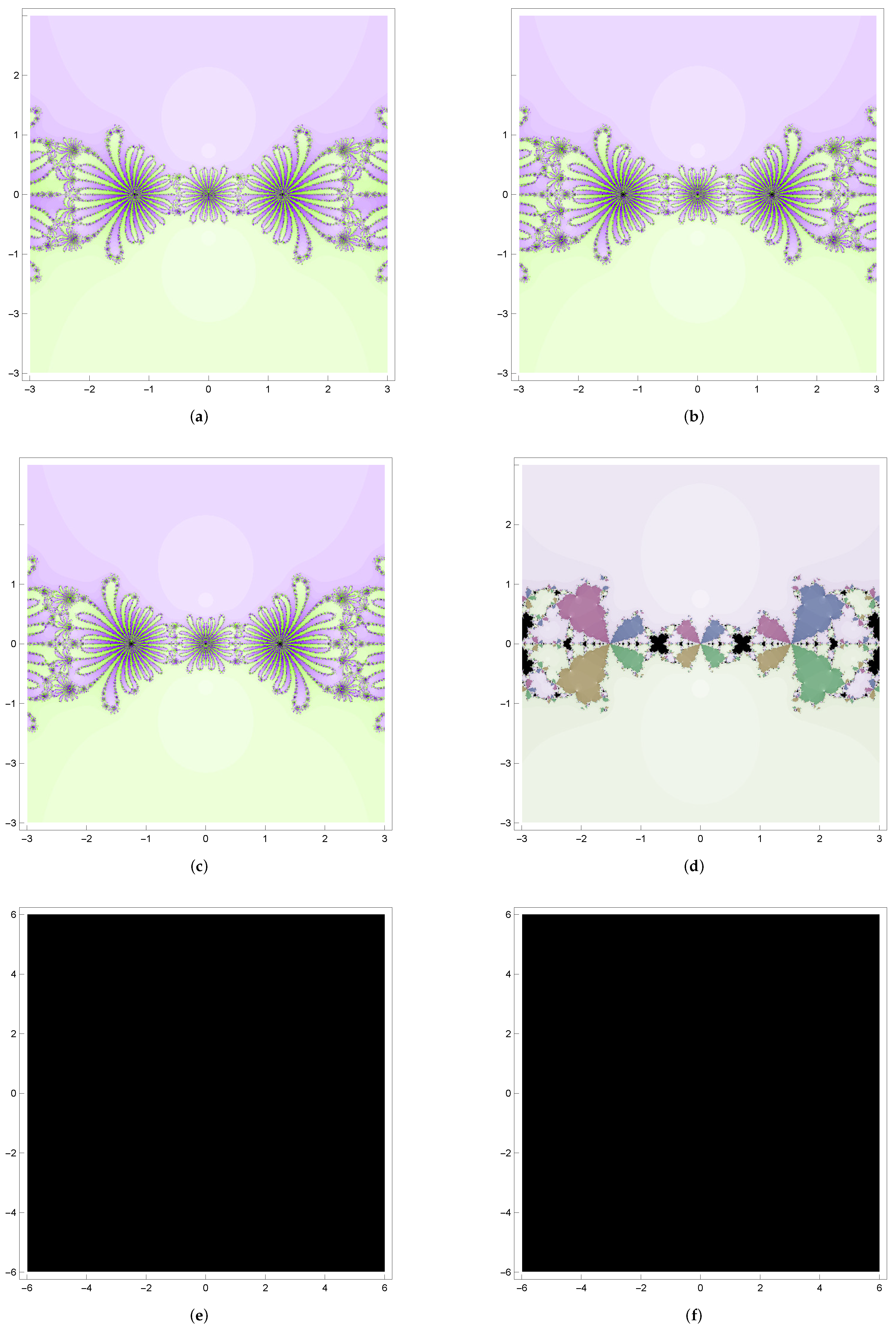
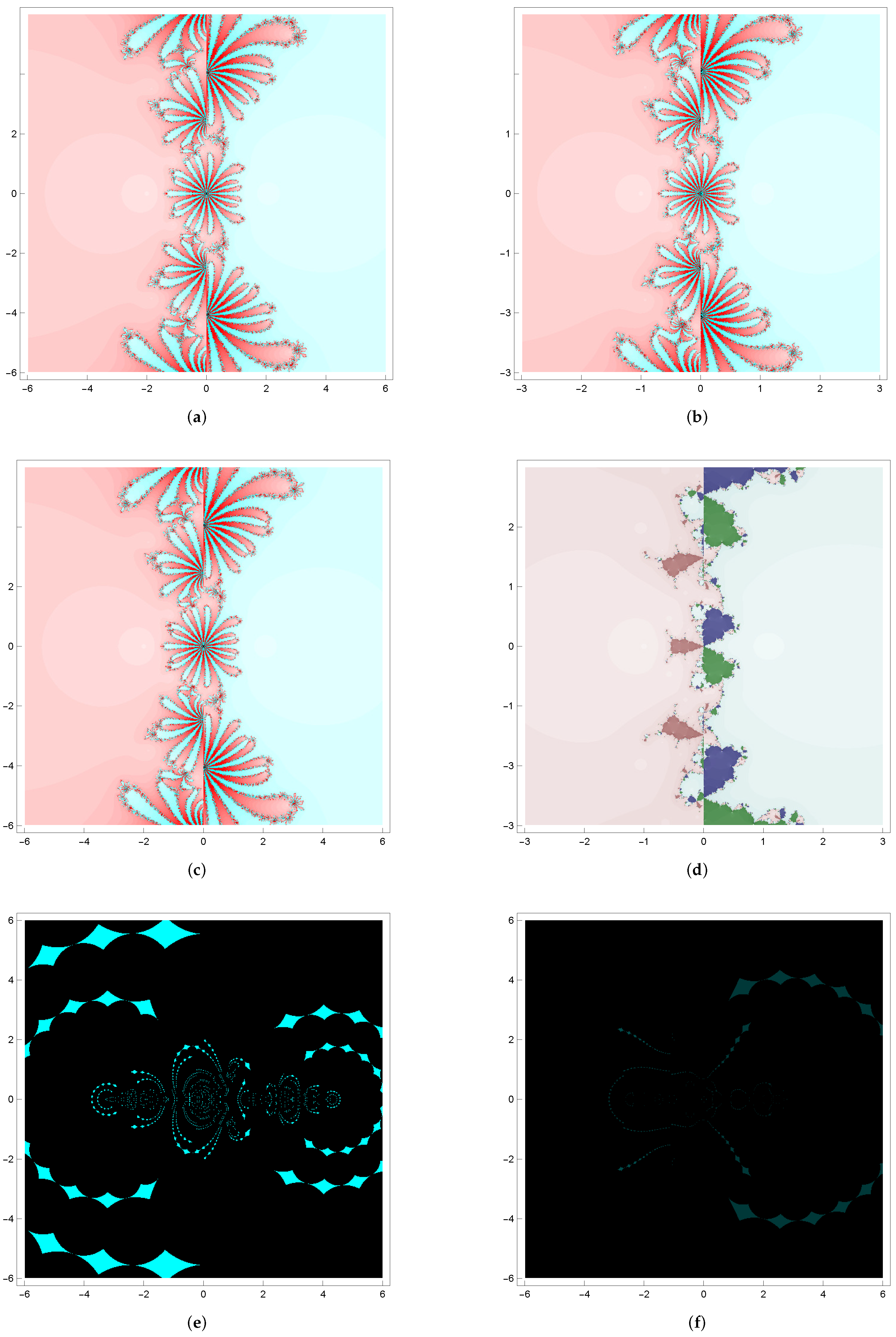
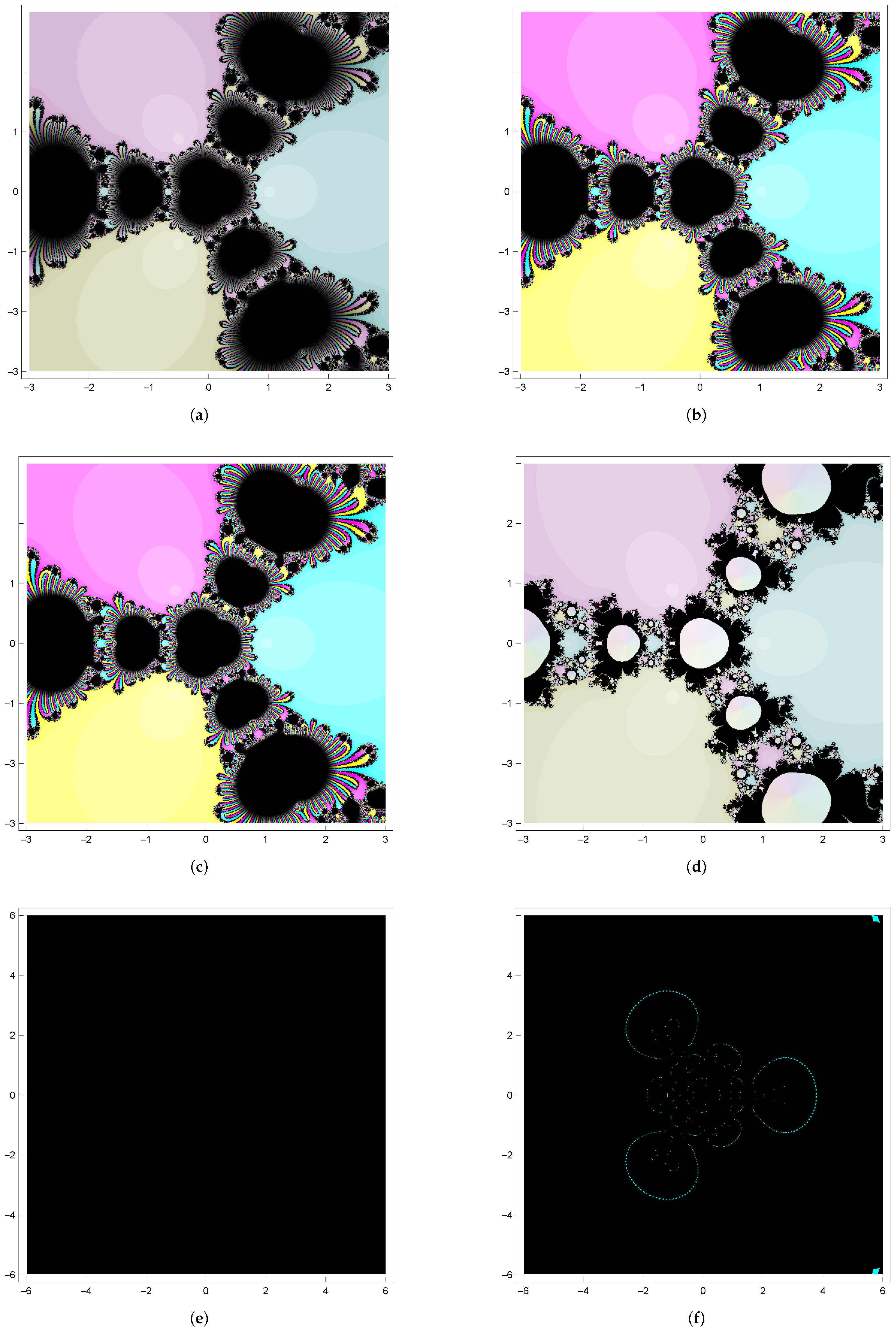
In Figure 1, Figure 2, Figure 3 and Figure 4, a six-by-six square region centered at the origin includes all the roots of the test functions. A $600\times 600$ uniform grid in this region is used to mark initial values for the iterative schemes to draw the basins of attraction. The grid point of a square is colored differently according to the number of iterations required for convergence. The point is colored in black if the methods do not converge.

Example 1.

We choose a quadratic polynomial raised to the power of two:

$$p_1\left(z\right)={(2z^2+1)}^2$$

with roots $\alpha =\pm 0.707107i$ with a multiplicity of 2. Basins of attraction for (M1), (M2), (M3), (M4), (X1), and (X2) are illustrated in Figure 1. Each basin is painted in various colors. Basins for $\alpha =+0.707107i$ are painted purple and basins for $\alpha =-0.707107i$ are painted green in Figure 1 (a)–(c). At zero, its color is light (white), while becoming darker for more iterative numbers required for convergence within the set iteration. Method (M1) performs better in terms of CPU, and M4 is better in terms of avg for $p_1\left(z\right)$. There are similar lobes along the boundaries of the basins in (a), (b), and (c). Picture (d) has colored (yellow, magenta, green, blue, and so on) carrot shapes around the boundary. Methods (X1) and (X2) do not have the value of the total convergent point, and pictures (e) and (f) show the black region.

Example 2.

As a second test example, we selected a quadratic polynomial raised to the power of three with all real roots:

$$p_2\left(z\right)={(z^2-1)}^3$$

The roots are $\alpha =\pm 1$ with a multiplicity of 3. Basins of attraction for (M1)-(X2) are illustrated in Figure 2. Method (M4) performs better in terms of avg. Basins for $\alpha =-1$ are painted red and basins for $\alpha =1$ are blue. There are similar lobes along the boundaries of the basins in Figure 2a–d has colored (blue, green, magenta) carrot shapes around the boundary. Methods (X1) and (X2) have considerable black points and circular patterns made up of blue diamond shapes in Figure 2e,f.

Example 3.

We choose a cubic polynomial raised to the power of two:

$$p_3\left(z\right)={(z^3-1)}^2,$$

with roots $\alpha =-0.5\pm 0.866025i,1$. Method (M4) is better regarding CPU and avg. The basins of method (X1) are represented by black regions and the basins of method (X2) are represented by circular light blue patterns in Figure 3.

The local convergence depends on the function, an initial value, the multiplicity, and a root. It cannot be said that one iterative method is always better than other methods. It is essential to choose an initial guess that guarantees the convergence of the numerical method. Deciding how close the initial guess should be to the root is not easy, as it depends on computational precision, the selected function, and the error bound. To choose a stable initial value, we can use basins of attraction in Figure 1, Figure 2, Figure 3 and Figure 4.

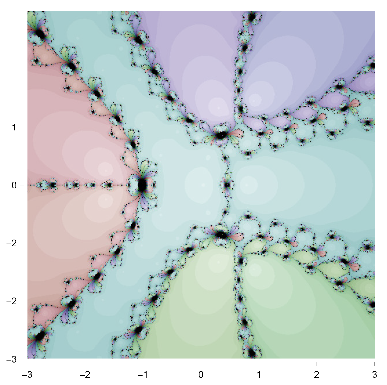
We use the equation in the blood rheology model [30]

$$f\left(x\right)={(\frac{x^8}{441}+\frac{8x^5}{63}-\frac{2,857,144,357x^4}{50,000,000,000}+\frac{16x^2}{9}-\frac{906,122,449x}{250,000,000}+\frac{3}{10})}^4$$

to carry out the experiment (M1) for the basins in Figure 4.

Substituting $A_0=A_1=1,A_2=2m/(-1+m),A_3=\lambda ,A_4=0,A_5=0$ and $B_{00}=B_{01}=B_{10}=1,B_{20}=2m/(-1+m),B_{11}=2,B_{21}=0,B_{30}=A_3=\lambda ,B_{40}=A_4=0$ into (24) to plot the convergent region, we select the following method, called (M5):

$$\left\{\begin{array}{c}{A}_f\left(k\right)=1+k+(2m/(-1+m))k^2+\lambda k^3,\hfill \\ B_f(k,v)=1+k+(2m/(-1+m))k^2+\lambda k^3+(1+2k)v,\hfill \end{array}\right.$$

(25)

Figure 5 shows the convergence region [31] of (M5) according to $\lambda =-2.375$ and $\lambda =-3.3305+0.0712i$.

4. Conclusions

Even though the proposed methods (M1)–(M4) are of the sixth order, like the existing methods (X1) and (X2), the number of divergent points for (M1)–(M4) is much smaller than for (X1) and (X2). The basins for (X1) and (X2) are black for $p_1\left(z\right)$ and the basins for (X1) and (X2) for $p_2\left(z\right)$ have some blue patterns but also a lot of black points. In summary, we find that the proposed methods are faster and require fewer iterations per point on average. It is important to choose the type of initial guess for the iterative schemes, ensuring it is chosen near the root for convergence. In future work, the fractal behavior behind the improved methods will be studied in more detail.

References

- Ahlfors, L.V. Complex Analysis; McGraw-Hill Book, Inc.: New York, NY, USA, 1979. [Google Scholar]
- Hörmander, L. An Introduction to Complex Analysis in Several Variables; North-Holland Publishing Company: Amsterdam, The Netherlands, 1973. [Google Scholar]
- Shabat, B.V. Introduction to Complex Analysis PART II, Functions of Several Variables; American Mathematical Society: Providence, RI, USA, 1992. [Google Scholar]
- Devaney, R.L. An Introduction to Chaotic Dynamical Systems; Addison-Wesley Publishing Company, Inc.: Boston, MA, USA, 1987. [Google Scholar]
- Kung, H.T.; Traub, J.F. Optimal order of one-point and multipoint iteration. J. Assoc. Comput. Mach. 1974, 21, 643–651. [Google Scholar] [CrossRef]
- Soleymani, F.; Babajee, D.K.R. Computing multiple zeros using a class of quartically convergent methods. Alex. Eng. J. 2013, 52, 531–541. [Google Scholar] [CrossRef]
- Chun, C.; Neta, B. Comparative study of eighth order methods for finding simple roots of nonlinear equations. Numer. Algorithms 2017, 74, 1169–1201. [Google Scholar] [CrossRef]
- Cordero, A.; Torresgrosa, J.R.; Vassileva, M.P. Three-step iterative methods with optimal eighth-order convergence. J. Comput. Appl. Math. 2011, 235, 3189–3194. [Google Scholar] [CrossRef]
- Geum, Y.H.; Kim, Y.I. A uniparametric family of three-step eighth-order multipoint iterative methods for simple roots. Appl. Math. Lett. 2011, 24, 929–935. [Google Scholar] [CrossRef]
- Liu, L.; Wang, X. Eighth-order methods with high efficiency index for solving nonlinear equations. Appl. Math. Comput. 2010, 15, 3449–3454. [Google Scholar] [CrossRef]
- Petković, M.S.; Neta, B.; Petković, L.D.; Džunić, J. Multipoint methods for solving nonlinear equations: A survey. Appl. Math. Comput. 2014, 226, 635–660. [Google Scholar] [CrossRef]
- Sharma, J.R.; Arora, H. A new family of optimal eighth order methods with dynamics for nonlinear equations. Appl. Math. Comput. 2016, 273, 924–933. [Google Scholar] [CrossRef]
- Traub, J.F. Iterative Methods for the Solution of Equations; Chelsea Publishing Company: Chelsea, VT, USA, 1982. [Google Scholar]
- Maroju, P.; Behl, R.; Motsa, S.S. Some novel and optimal families of King’s method with eighth and sixteenth-order of convergence. J. Comput. Appl. Math. 2017, 318, 136–148. [Google Scholar] [CrossRef]
- Sharma, J.R.; Argyros, I.K.; Kumar, D. On a general class of optimal order multipoint methods for solving nonlinear equations. J. Math. Anal. Appl. 2017, 449, 994–1014. [Google Scholar] [CrossRef]
- Li, S.G.; Cheng, L.Z.; Neta, B. Some fourth-order nonliear solvers with closed formulae for multiple roots. Comput. Math. Appl. 2010, 59, 126–135. [Google Scholar] [CrossRef]
- Liu, B.; Zhou, X. A new family of fourth-order methods for mulltiple roots of nonlinear equations. Nonlinear Anal. Model. Contral 2013, 18, 143–152. [Google Scholar] [CrossRef]
- Magreñán, A.A.; Cordero, A.; Gitiérrez, J.M.; Torregrosa, J.R. Real qualitative behavior of a fourth-order family of iterative methods by using the convergence plane. Math. Comput. Simulat. 2014, 105, 49–61. [Google Scholar] [CrossRef]
- Magreñán, A.A. Different anomalies in a Jarratt family of iterative root-finding methods. Appl. Math. Comput. 2014, 233, 29–38. [Google Scholar] [CrossRef]
- Geum, Y.H. Study on the dynamical analysis of a family of third order multiple-zero finders. Eur. J. Pure Appl. Math. 2023, 16, 2775–2785. [Google Scholar] [CrossRef]
- Neta, B.; Scott, N.; Chun, C. Basins of attractors for various methods for multiple root. Appl. Math. Comput. 2012, 218, 5043–5066. [Google Scholar] [CrossRef]
- Neta, B.; Chun, C. On a family of Laguerre methods to find multiple roots of nonlinear equations. Appl. Math. Comput. 2013, 219, 10987–11004. [Google Scholar] [CrossRef]
- Neta, B.; Johnson, A.N. High order nonliear solver for multiple roots. Comput. Math. Appl. 2008, 55, 2012–2017. [Google Scholar] [CrossRef]
- Neta, B. Extension of Murakami’s high order nonlinear solver to multiple roots. Int. J. Comput. Math. 2010, 8, 1023–1031. [Google Scholar] [CrossRef]
- Neta, B.; Chun, C.; Scott, M. Basins of attraction for optimal eighth order methods to find simple roots of nonlinear equations. Appl. Math. Comput. 2014, 227, 567–592. [Google Scholar] [CrossRef]
- Neta, B.; Chun, C. Basins of attraction for several optimal fourth order methods for multiple roots. Math. Comput. Simul. 2014, 103, 39–59. [Google Scholar] [CrossRef]
- Geum, Y.H.; Kim, Y.I.; Neta, B. A class of two-point sixth-order multiple-zero finders of modified double-Newton type and their dynamics. Appl. Math. Comput. 2015, 270, 387–400. [Google Scholar] [CrossRef]
- Geum, Y.H.; Kim, Y.I.; Neta, B. A sixth-order family of three-point modified Newton-like multiple-root finders and the dynamics behind their extraneous fixed points. Appl. Math. Comput. 2016, 283, 120–140. [Google Scholar] [CrossRef]
- Wolfram, S. The Mathematica Book, 5th ed.; Wolfram Media: Champaign, IL, USA, 2003. [Google Scholar]
- Fournier, R.L. Basic Transport Phenomena in Biomedical Engineering; CRC Press: Boca Raton, FL, USA, 2017. [Google Scholar]
- Deng, J.J.; Chiang, H.D. Convergence Region of Newton Iterative Power Flow Method: Numerical Studies. J. Appl. Math. 2013, 2013, 509496. [Google Scholar] [CrossRef]