
Load Distribution Analysis and Contact Stiffness Prediction of the Dual-Drive Ball Screw Pair Considering Guide Rail Geometric Error and Slide Position

Abstract
:1. Introduction
2. Axial Load Offset Analysis of the Dual-Drive Ball Screw Pair
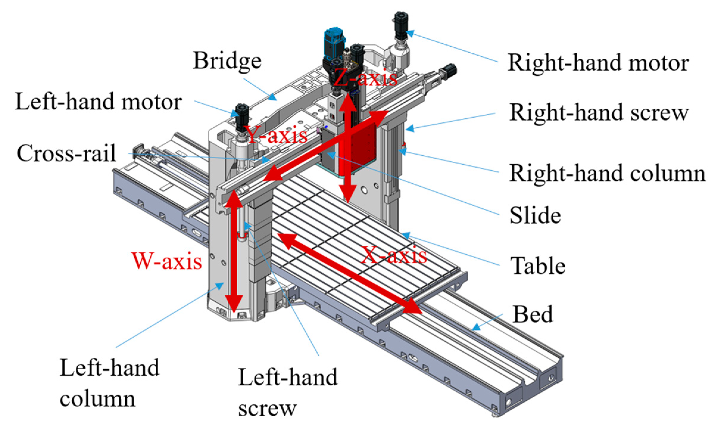
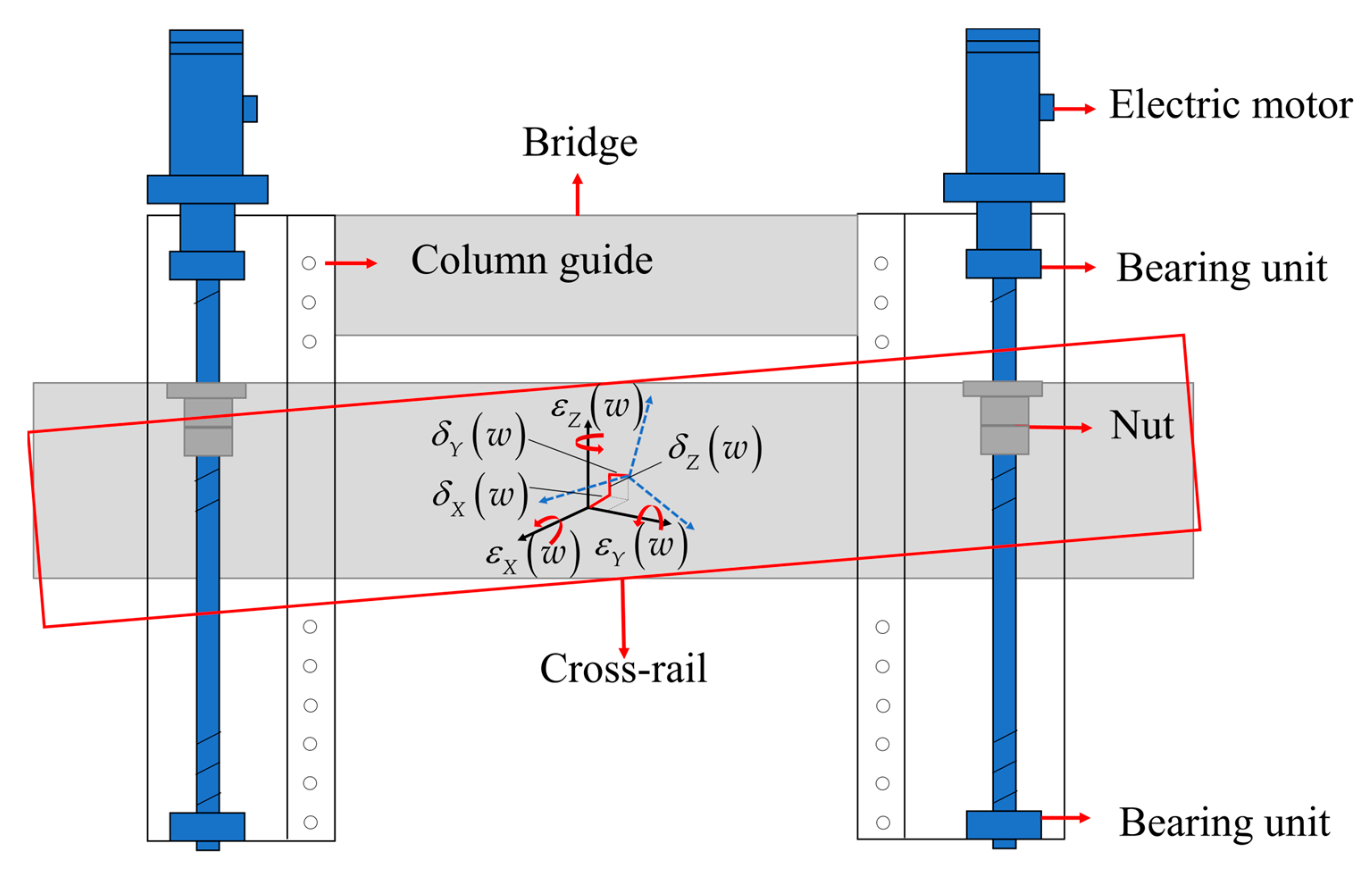
2.1. Structure Introduction of Machine Tool
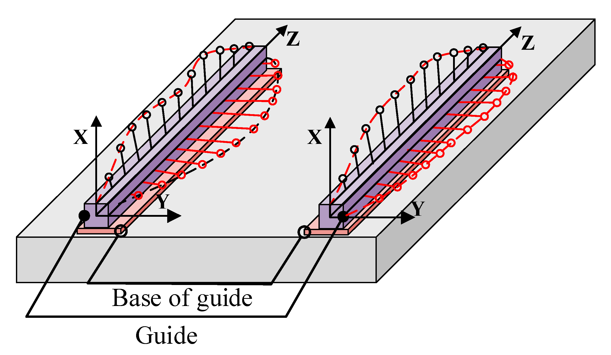
2.2. Mapping Relationship between Guide Tolerance and Geometric Error
2.3. Offset Analysis of Dual-Drive Ball Screw Pair
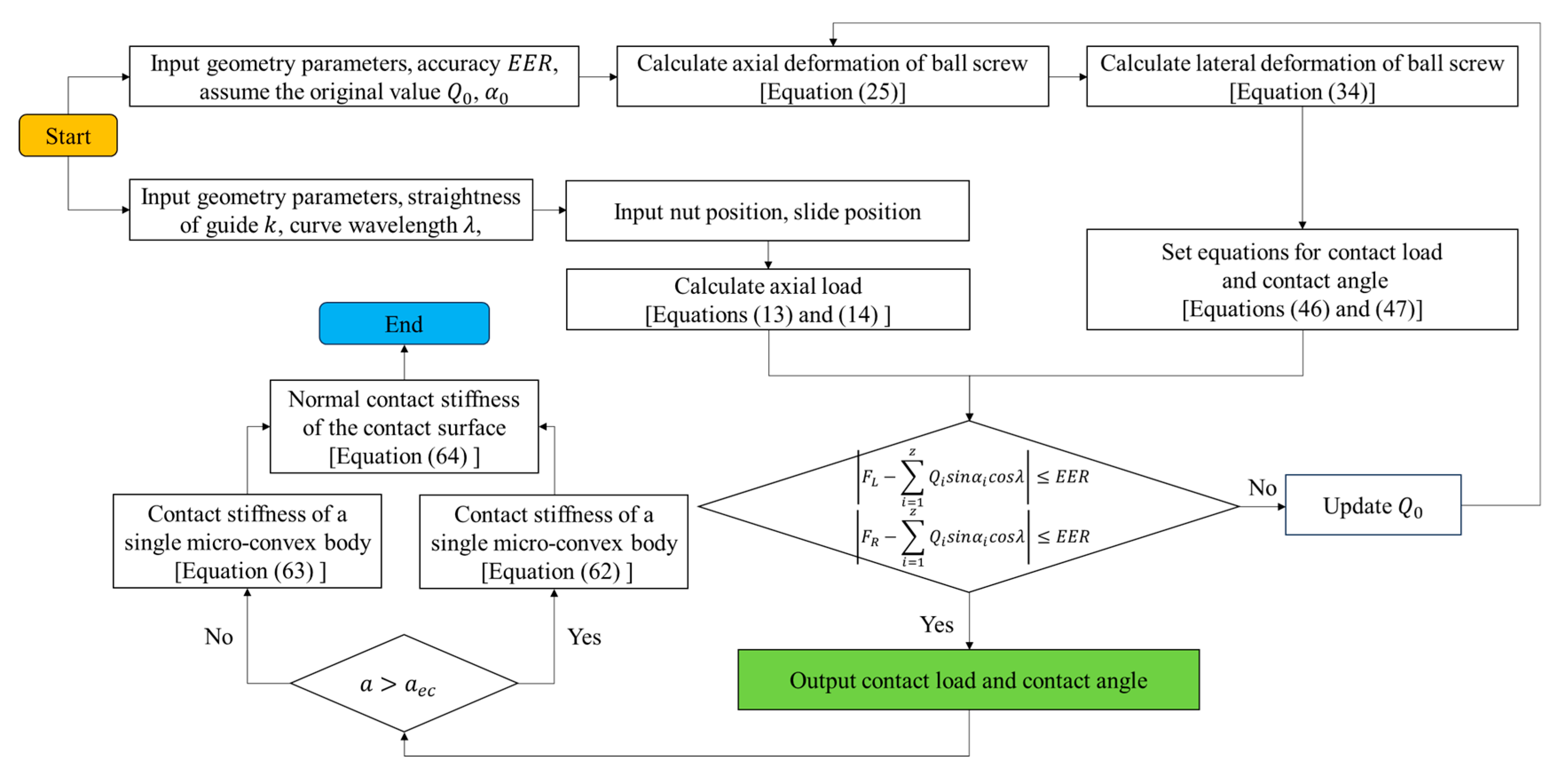
3. Contact Load Distribution Modeling and Verification Analysis
3.1. Axial Deformation of Ball Screw during Movement
3.2. Relation between Contact Angle and Elastic Deformation
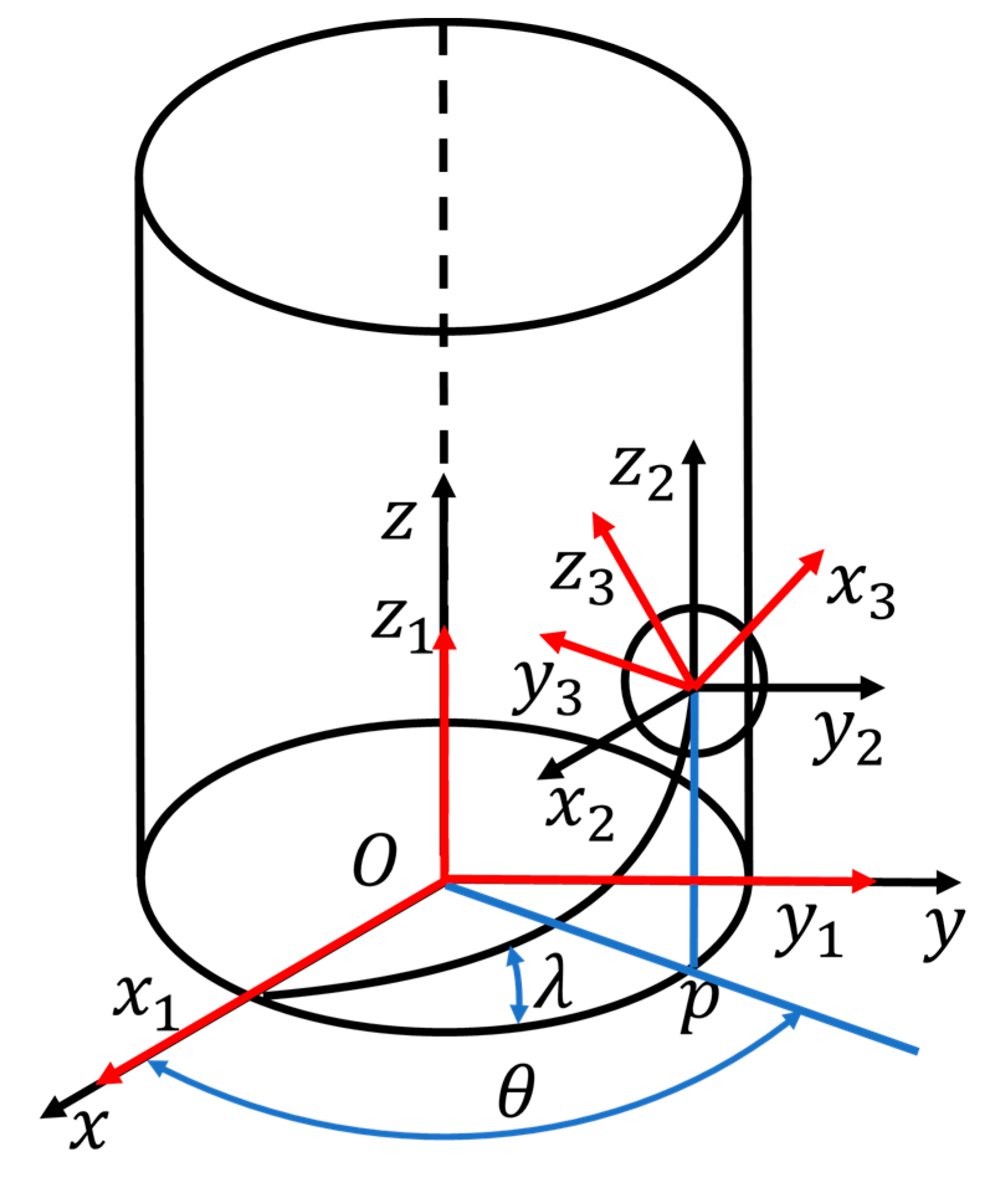
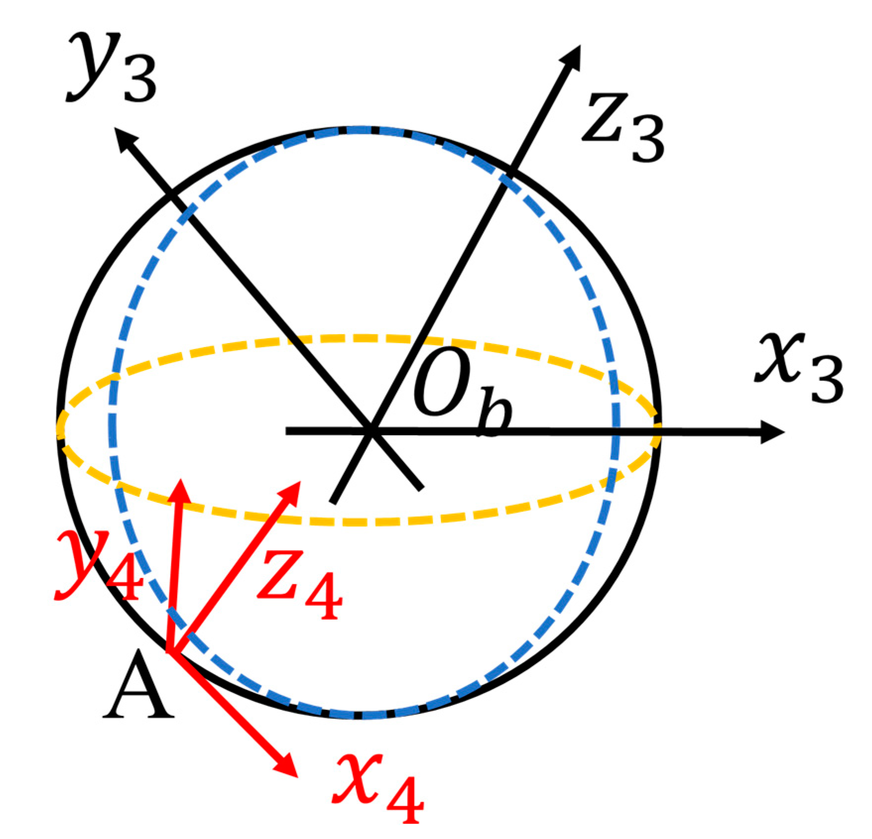
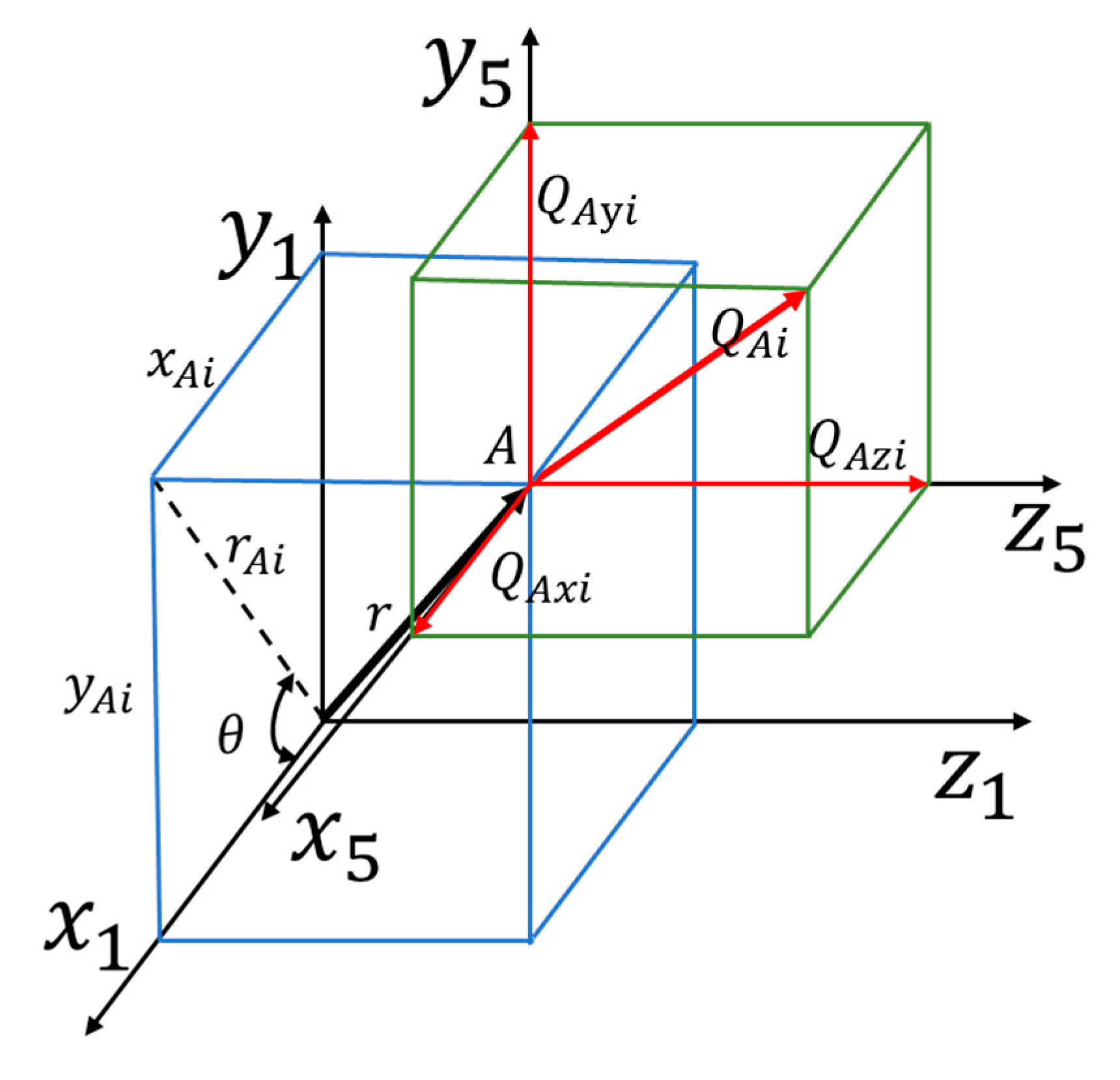
3.3. Homogeneous Co-Ordinate Transformation
3.4. Lateral Deformation Analysis of the Ball Screw
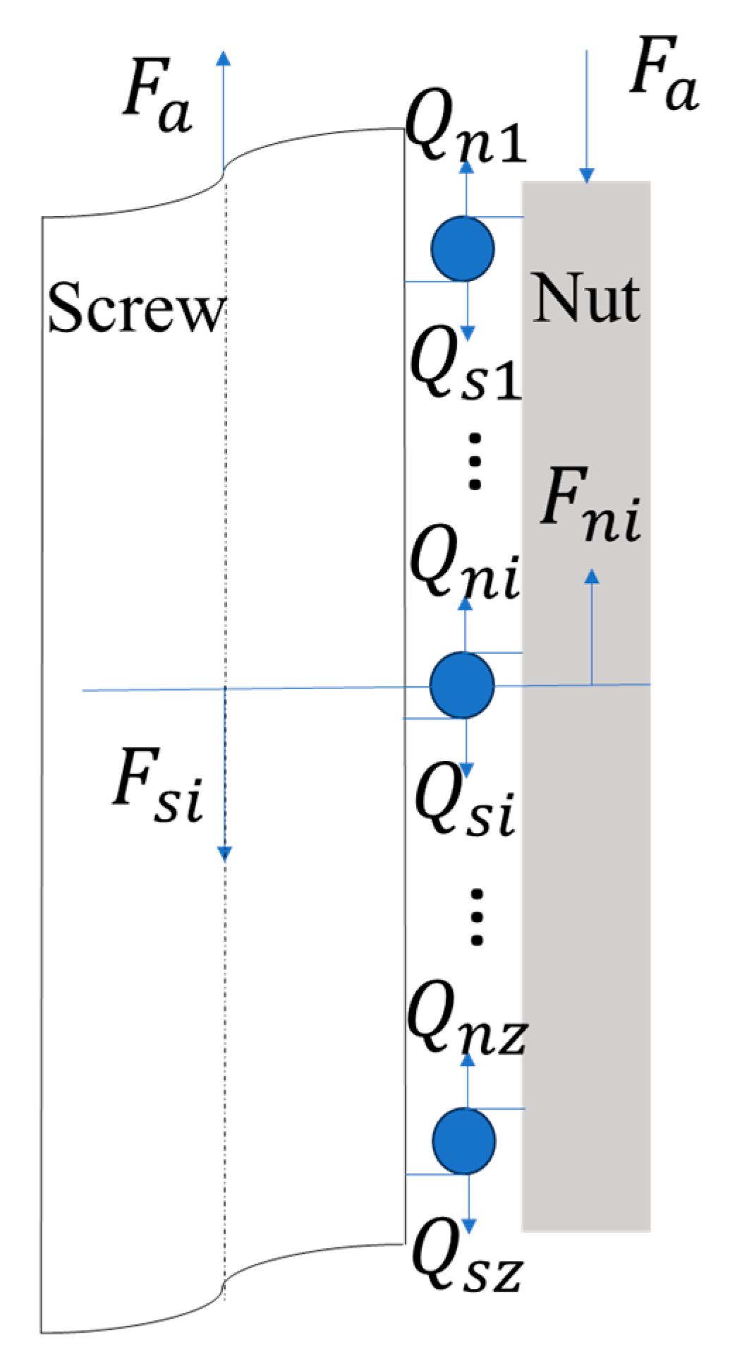
3.5. The Contact Load Modeling of the Ball Screw
3.6. Modeling of the Contact Stiffness Based on Fractal Theory
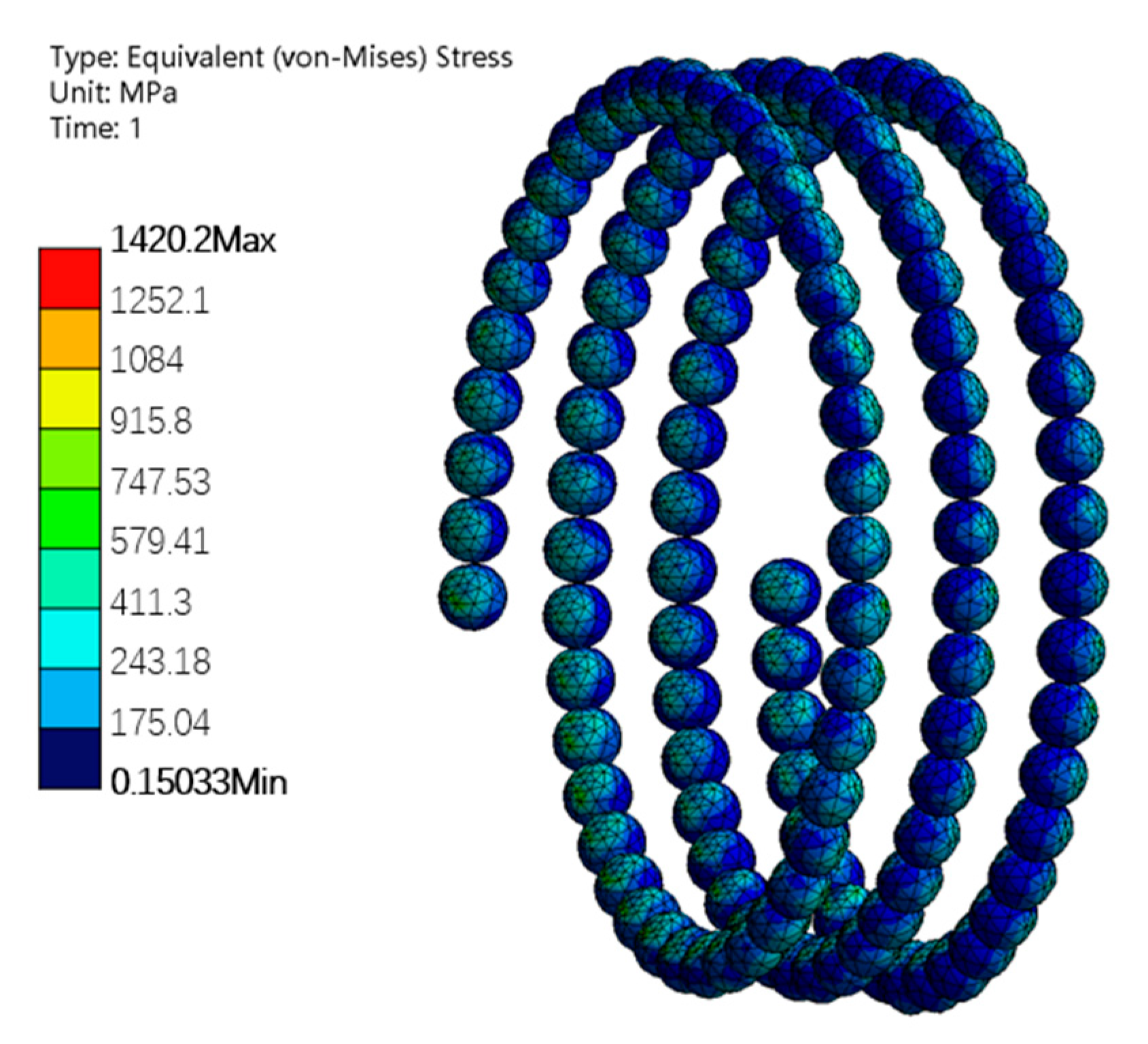
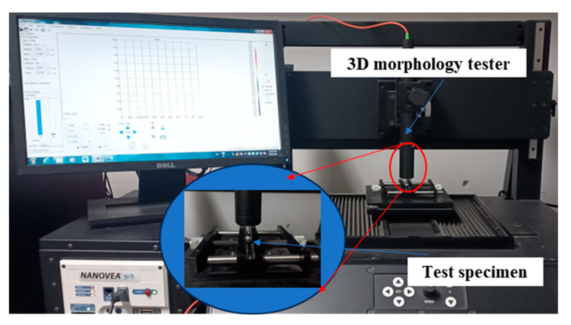
3.7. Finite Element Verification
4. Results and Discussion
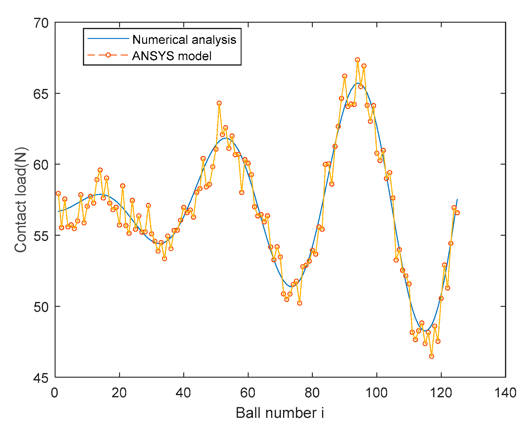
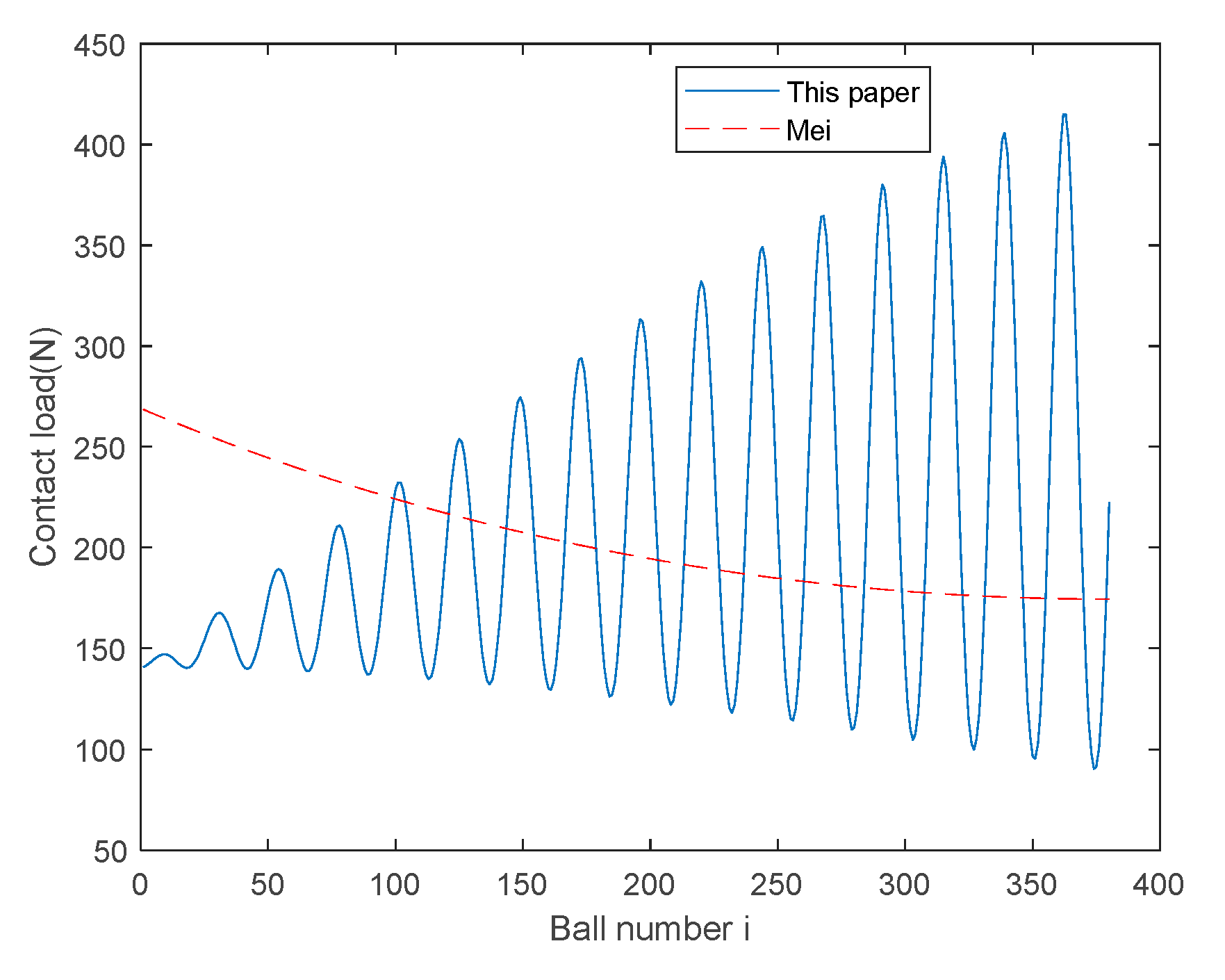
4.1. Verification of the Proposed Model
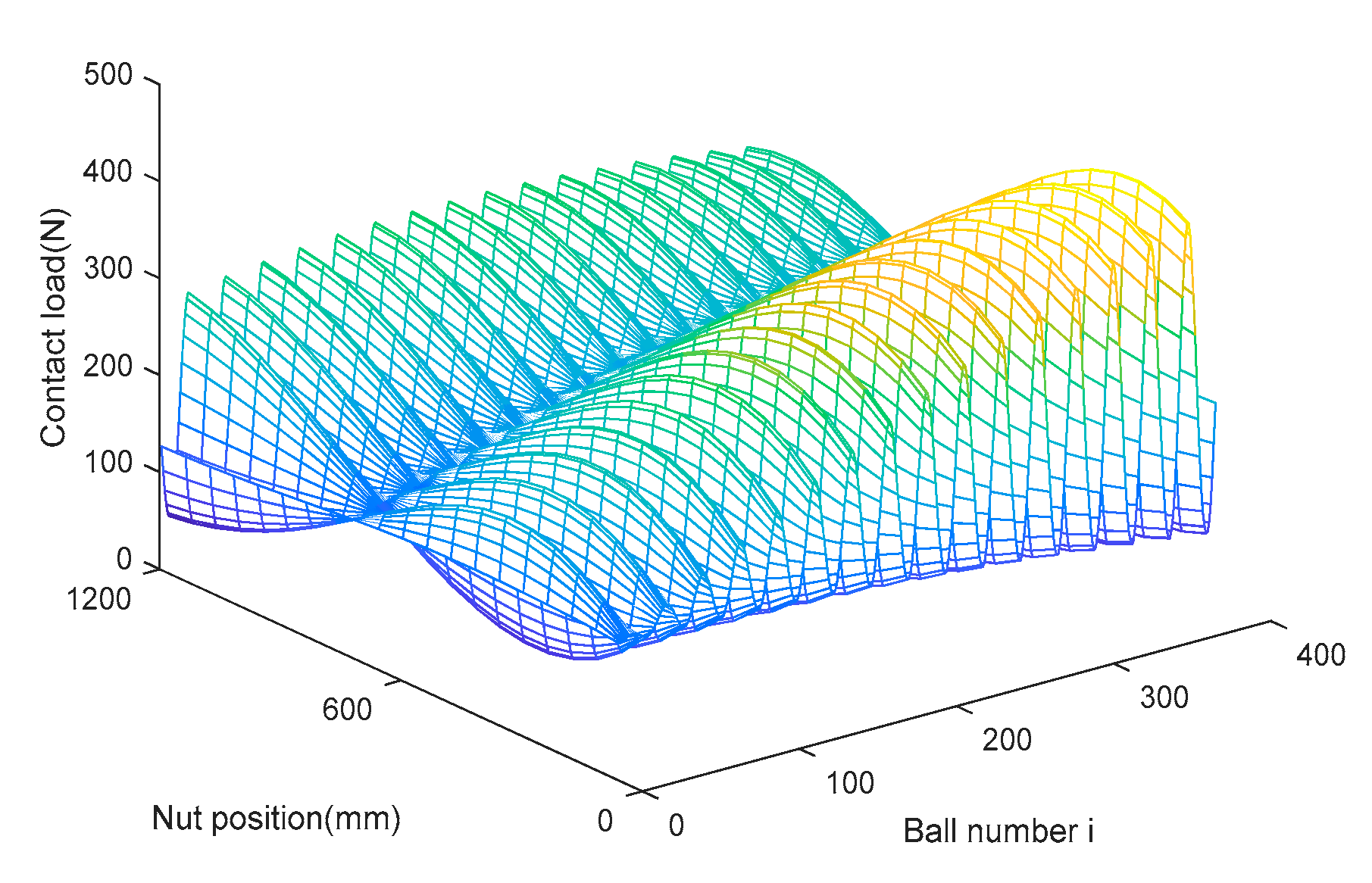
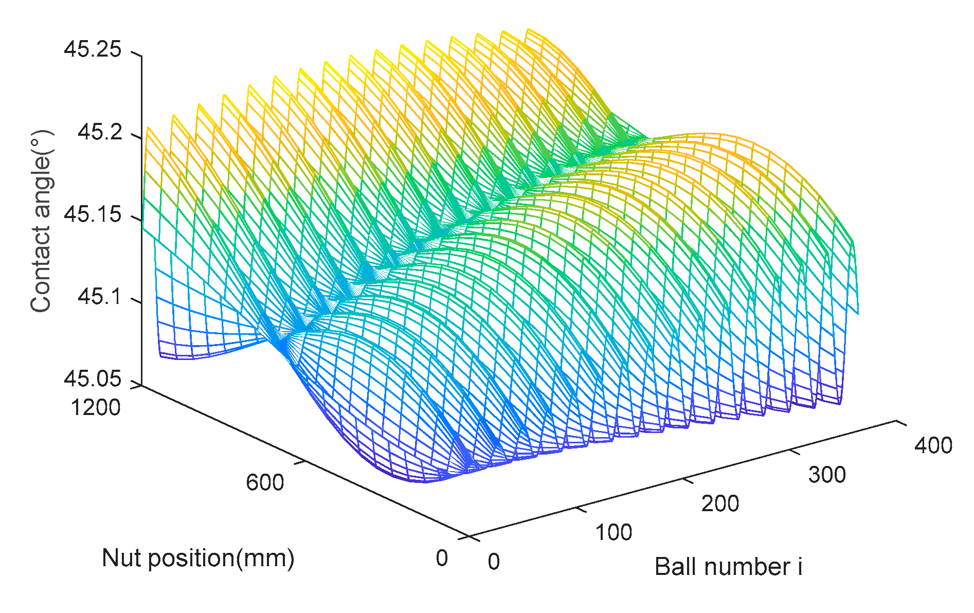
4.2. Distribution Analysis of Contact Load/Angle with Ball Screw Positions
4.3. Distribution Analysis of Contact Load Based on Multiple Influencing Factors
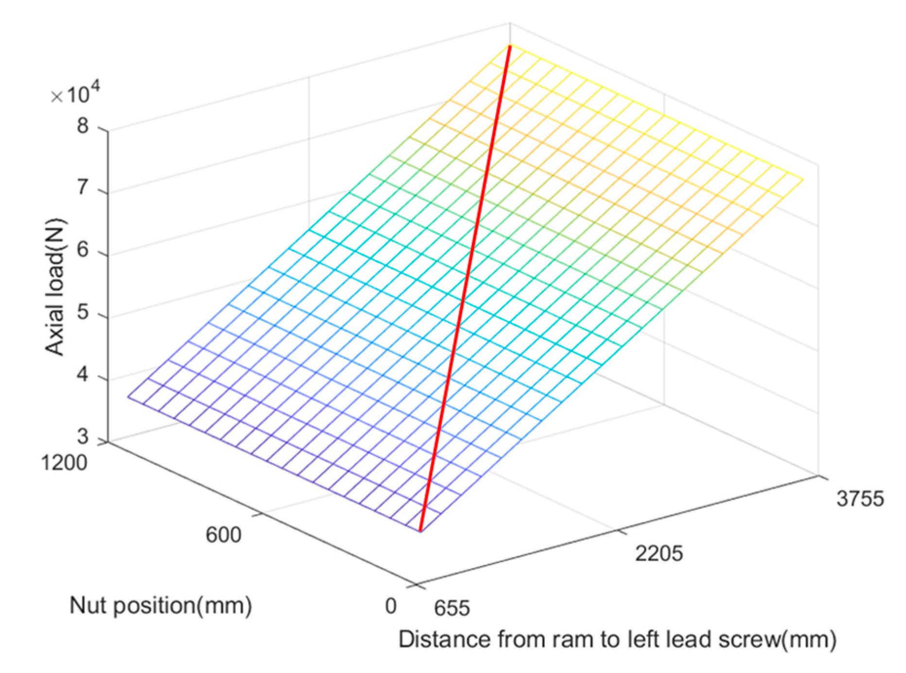
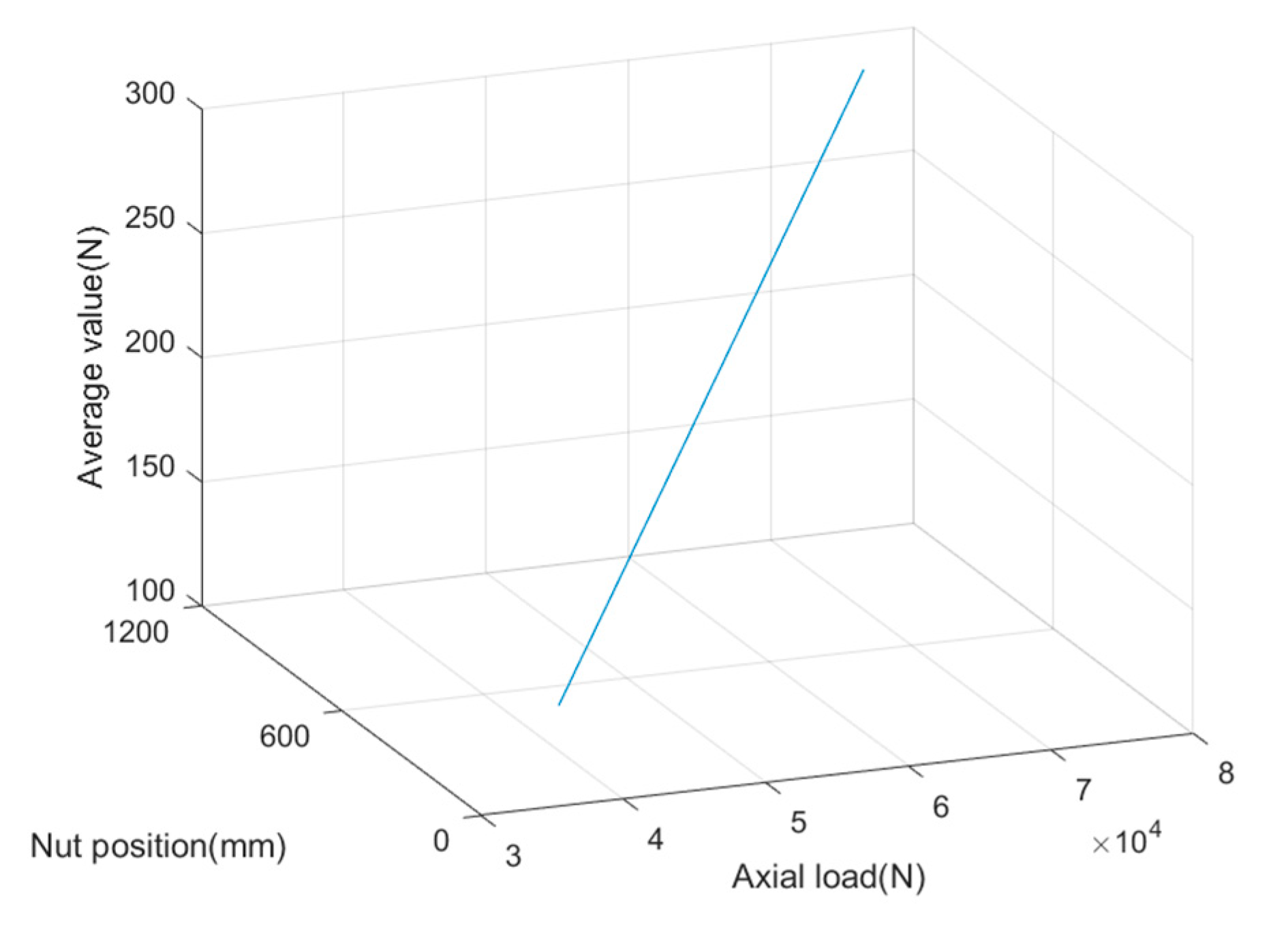
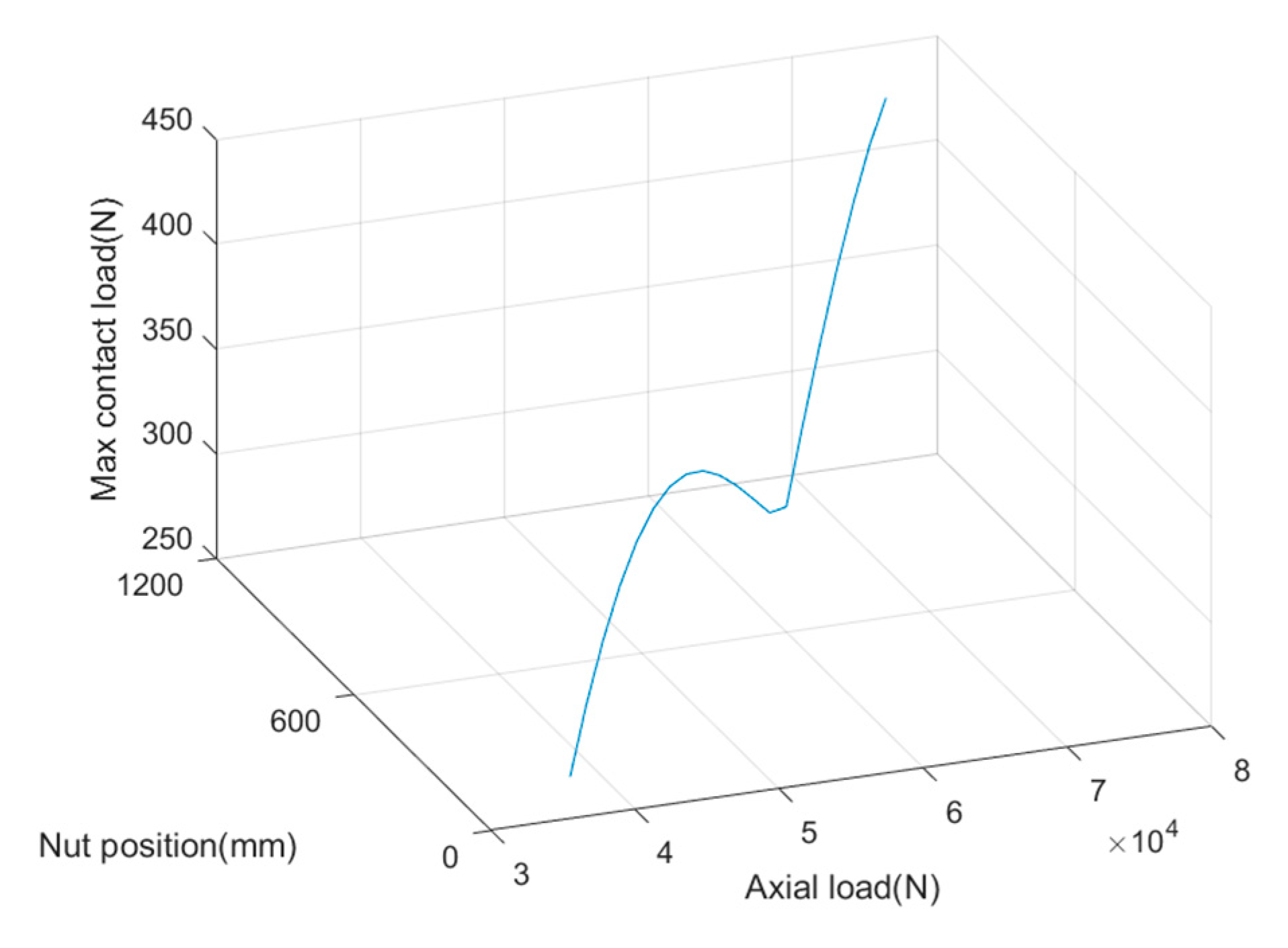
4.4. Axial Load Change on Dual-Drive Ball Screw Pair
4.5. Distribution of Contact Load and Contact Angle under an Offset
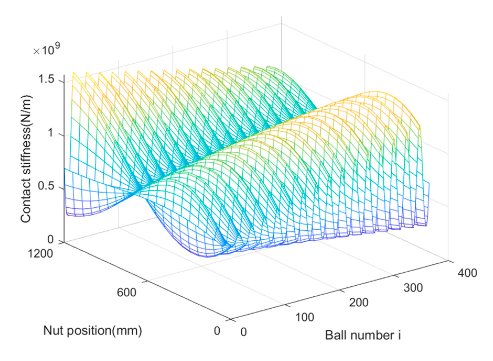
4.6. Contact Stiffness Analysis of Ball Screw Pair
5. Conclusions
- (1)
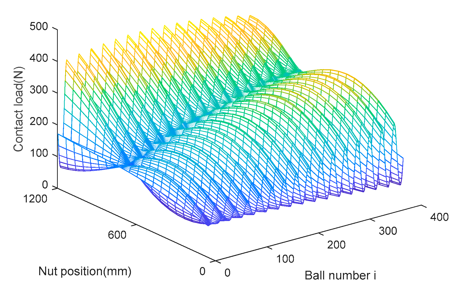
- The distribution curves of contact load and contact angle for nuts at different positions along the screw exhibit distinct variations, displaying complex nonlinear characteristics across the feed direction of the screw. The uneven contact load distribution in the middle position of the nut is superior to that at the screw ends. When the nut is located at the upper, middle, and lower end of the screw, the standard deviation of the contact load distribution is 78.38, 30.05, and 64.98, respectively. And the standard deviation of the contact angle distribution is 0.0337, 0.0130, and 0.0285, respectively.
- (2)
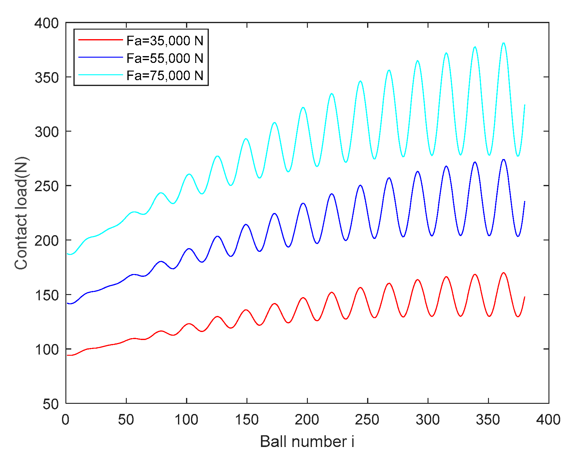
- There is a similar evolutionary trend between contact load and axial load, as well as between contact angle and axial load. The unevenness of contact load distribution and contact angle distribution increases with the increase in axial load. When the axial load is 35,000 N/55,000 N/75,000 N, the standard deviation of the contact load distribution is 18.71/32.74/37.95 and the standard deviation of the contact angle distribution is 0.0096/0.0144/0.0191.
- (3)
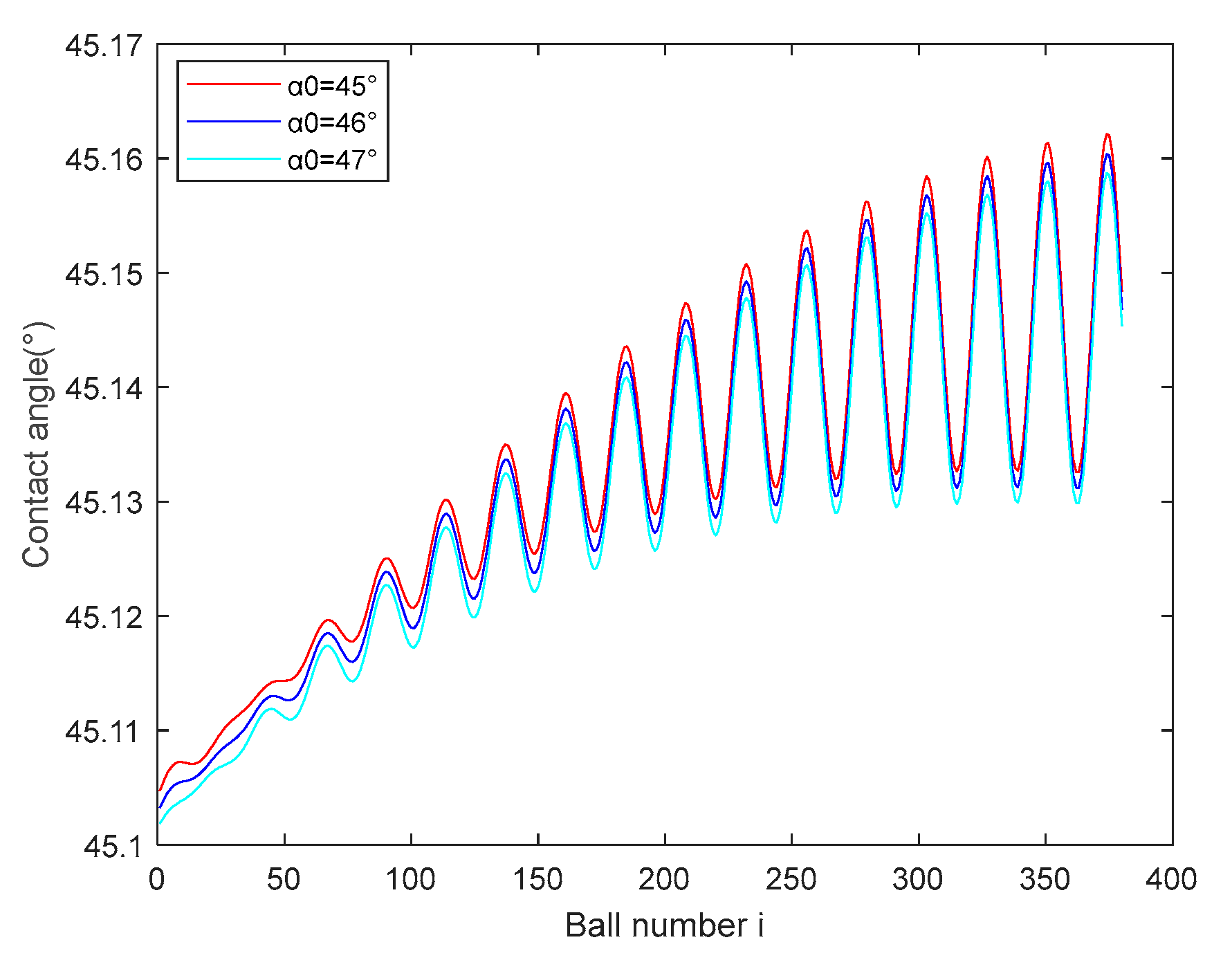
- The standard deviations of contact load distribution at different initial contact angles (, , and ) are 32.74, 32.44, and 32.17, respectively, indicating a decreasing trend. The standard deviations of the contact angle distribution are constant, which is 0.0144.
- (4)
- Due to the influence of guide rail geometric error and slide position, the contact stiffness of the double-drive ball screw pair shows complex nonlinearity as well.
Author Contributions
Funding
Data Availability Statement
Acknowledgments
Conflicts of Interest
References
- Huang, S.; Wang, S. Mechatronics and Control of a Long-Range Nanometer Positioning Servomechanism. Mechatronics 2009, 19, 14–28. [Google Scholar] [CrossRef]
- Cheng, Q.; Qi, B.; Liu, Z.; Zhang, C.; Xue, D. An Accuracy Degradation Analysis of Ball Screw Mechanism Considering Time-Varying Motion and Loading Working Conditions. Mech. Mach. Theory 2019, 134, 1–23. [Google Scholar] [CrossRef]
- Li, Y.; Mu, L.; Gao, P. Particle Swarm Optimization Fractional Slope Entropy: A New Time Series Complexity Indicator for Bearing Fault Diagnosis. Fractal Fract. 2022, 6, 345. [Google Scholar] [CrossRef]
- Liu, C.; Zhao, C.; Meng, X.; Wen, B. Static Load Distribution Analysis of Ball Screws with Nut Position Variation. Mech. Mach. Theory 2020, 151, 103893. [Google Scholar] [CrossRef]
- Qi, B.; Zhao, J.; Chen, C.; Song, X.; Jiang, H. Accuracy Decay Mechanism of Ball Screw in CNC Machine Tools for Mixed Sliding-Rolling Motion under Non-Constant Operating Conditions. Int. J. Adv. Manuf. Technol. 2023, 124, 4349–4363. [Google Scholar] [CrossRef]
- Li, Y.; Tang, B.; Geng, B.; Jiao, S. Fractional Order Fuzzy Dispersion Entropy and Its Application in Bearing Fault Diagnosis. Fractal Fract. 2022, 6, 544. [Google Scholar] [CrossRef]
- Meng, J.; Du, X.; Li, Y.; Chen, P.; Xia, F.; Wan, L. A Multiscale Accuracy Degradation Prediction Method of Planetary Roller Screw Mechanism Based on Fractal Theory Considering Thread Surface Roughness. Fractal Fract. 2021, 5, 237. [Google Scholar] [CrossRef]
- Nastac, S. On Vibration Joint Time-Frequency Investigations of CNC Milling Machines for Tool Trajectory Task Conformity Estimation. Shock Vib. 2018, 2018, 7375057. [Google Scholar] [CrossRef]
- Tang, H.; Duan, J.; Zhao, Q. A Systematic Approach on Analyzing the Relationship between Straightness & Angular Errors and Guideway Surface in Precise Linear Stage. Int. J. Mach. Tools Manuf. 2017, 120, 12–19. [Google Scholar]
- Wang, Z.; Wang, D.; Wu, Y.; Dong, H.; Yu, S. Error Calibration of Controlled Rotary Pairs in Five-Axis Machining Centers Based on the Mechanism Model and Kinematic Invariants. Int. J. Mach. Tools Manuf. 2017, 120, 1–11. [Google Scholar] [CrossRef]
- Qiao, Y.; Chen, Y.; Yang, J.; Chen, B. A Five-Axis Geometric Errors Calibration Model Based on the Common Perpendicular Line (CPL) Transformation Using the Product of Exponentials (POE) Formula. Int. J. Mach. Tools Manuf. 2017, 118–119, 49–60. [Google Scholar] [CrossRef]
- Huang, N.; Jin, Y.; Bi, Q.; Wang, Y. Integrated Post-Processor for 5-Axis Machine Tools with Geometric Errors Compensation. Int. J. Mach. Tools Manuf. 2015, 94, 65–73. [Google Scholar] [CrossRef]
- Feng, W.L.; Yao, X.D.; Azamat, A.; Yang, J.G. Straightness Error Compensation for Large CNC Gantry Type Milling Centers Based on B-Spline Curves Modeling. Int. J. Mach. Tools Manuf. 2015, 88, 165–174. [Google Scholar] [CrossRef]
- Niu, P.; Cheng, Q.; Zhang, T.; Yang, C.; Zhang, Z.; Liu, Z. Hyperstatic Mechanics Analysis of Guideway Assembly and Motion Errors Prediction Method under Thread Friction Coefficient Uncertainties. Tribol. Int. 2023, 180, 108275. [Google Scholar] [CrossRef]
- Hwang, J.; Park, C.; Gao, W.; Kim, S. A Three-Probe System for Measuring the Parallelism and Straightness of a Pair of Rails for Ultra-Precision Guideways. Int. J. Mach. Tools Manuf. 2007, 47, 1053–1058. [Google Scholar] [CrossRef]
- Feng, G.; Pan, Y. Investigation of Ball Screw Preload Variation Based on Dynamic Modeling of a Preload Adjustable Feed-Drive System and Spectrum Analysis of Ball-Nuts Sensed Vibration Signals. Int. J. Mach. Tools Manuf. 2012, 52, 85–96. [Google Scholar] [CrossRef]
- Ekinci, T.; Mayer, J. Relationships between Straightness and Angular Kinematic Errors in Machines. Int. J. Mach. Tools Manuf. 2007, 47, 1997–2004. [Google Scholar] [CrossRef]
- Zha, J.; Xue, F.; Chen, Y. Straightness Error Modeling and Compensation for Gantry Type Open Hydrostatic Guideways in Grinding Machine. Int. J. Mach. Tools Manuf. 2017, 112, 1–6. [Google Scholar] [CrossRef]
- Mei, X.; Tsutsumi, M.; Tao, T.; Sun, N. Study on the Load Distribution of Ball Screws with Errors. Mech. Mach. Theory 2003, 38, 1257–1269. [Google Scholar] [CrossRef]
- Wei, C.; Lin, J. Kinematic Analysis of the Ball Screw Mechanism Considering Variable Contact Angles and Elastic Deformations. J. Mech. Des. 2003, 125, 717–733. [Google Scholar] [CrossRef]
- Gu, J.; Zhang, Y. Dynamic Analysis of a Ball Screw Feed System with Time-Varying and Piecewise-Nonlinear Stiffness. Proc. Inst. Mech. Eng. Part C J. Mech. Eng. Sci. 2019, 233, 6503–6518. [Google Scholar] [CrossRef]
- Lin, M.; Ravani, B.; Velinsky, S. Kinematics of the Ball Screw Mechanism. J. Mech. Des. 1994, 116, 849–855. [Google Scholar] [CrossRef]
- Hu, J.; Wang, M.; Zan, T. The Kinematics of Ball-Screw Mechanisms via the Slide–Roll Ratio. Mech. Mach. Theory 2014, 79, 158–172. [Google Scholar] [CrossRef]
- Huang, H.; Tsai, M.; Huang, Y. Modeling and Elastic Deformation Compensation of Flexural Feed Drive System. Int. J. Mach. Tools Manuf. 2018, 132, 96–112. [Google Scholar] [CrossRef]
- Zhou, C.; Feng, H.; Chen, Z.; Ou, Y. Correlation between Preload and No-Load Drag Torque of Ball Screws. Int. J. Mach. Tools Manuf. 2016, 102, 35–40. [Google Scholar] [CrossRef]
- Liu, J.; Feng, H.; Zhou, C. Static Load Distribution and Axial Static Contact Stiffness of a Preloaded Double-Nut Ball Screw Considering Geometric Errors. Mech. Mach. Theory 2022, 167, 104460. [Google Scholar] [CrossRef]
- Zhao, J.; Lin, M.; Song, X.; Guo, Q. Investigation of Load Distribution and Deformations for Ball Screws with the Effects of Turning Torque and Geometric Errors. Mech. Mach. Theory 2019, 141, 95–116. [Google Scholar] [CrossRef]
- ISO 230-1:2012; Test Code for Machine Tools—Part 1: Geometric Accuracy of Machines Operating under No-Load or Quasi-static Conditions. ISO: Geneva, Switzerland, 2012.
- Lin, M.; Velinsky, S.; Ravani, B. Design of the Ball Screw Mechanism for Optimal Efficiency. J. Mech. Des. 1994, 116, 856–861. [Google Scholar] [CrossRef]
- Wei, C.; Lin, J.; Horng, J. Analysis of a Ball Screw with a Preload and Lubrication. Tribol. Int. 2009, 42, 1816–1831. [Google Scholar] [CrossRef]
- Zhao, H.; Wu, Q. Application Study of Fractal Theory in Mechanical Transmission. Chin. J. Mech. Eng. 2016, 29, 871–879. [Google Scholar] [CrossRef]
- Zhao, Y.; Wu, H.; Liu, Z.; Cheng, Q.; Yang, C. A Novel Nonlinear Contact Stiffness Model of Concrete–Steel Joint Based on the Fractal Contact Theory. Nonlinear Dyn. 2018, 94, 151–164. [Google Scholar] [CrossRef]
- Liu, J.; Ma, C.; Wang, S. Precision Loss Modeling Method of Ball Screw Pair. Mech. Syst. Signal Process. 2020, 135, 106397. [Google Scholar] [CrossRef]


| Parameters | Value | Unit |
|---|---|---|
| Ball radius | 6.35 | mm |
| Screw groove radius | 6.985 | mm |
| Nut groove radius | 6.985 | mm |
| Length of screw | 1200 | mm |
| Nominal pitch circle radius | 50 | mm |
| Nominal pitch | 16 | mm |
| Number of balls | 380 | / |
| Outer diameter of nut | 155 | mm |
| Length of nut | 311 | mm |
| Elastic modulus | 210×109 | Pa |
| Poisson ratio | 0.3 | / |
| Helix angle | 2.9155 | degree |
Disclaimer/Publisher’s Note: The statements, opinions and data contained in all publications are solely those of the individual author(s) and contributor(s) and not of MDPI and/or the editor(s). MDPI and/or the editor(s) disclaim responsibility for any injury to people or property resulting from any ideas, methods, instructions or products referred to in the content. |
© 2023 by the authors. Licensee MDPI, Basel, Switzerland. This article is an open access article distributed under the terms and conditions of the Creative Commons Attribution (CC BY) license (https://creativecommons.org/licenses/by/4.0/).
Share and Cite
Liu, Z.; Zuo, W.; Qi, B.; Chen, C.; Guo, J.; Li, D.; Gao, S. Load Distribution Analysis and Contact Stiffness Prediction of the Dual-Drive Ball Screw Pair Considering Guide Rail Geometric Error and Slide Position. Fractal Fract. 2023, 7, 873. https://doi.org/10.3390/fractalfract7120873
Liu Z, Zuo W, Qi B, Chen C, Guo J, Li D, Gao S. Load Distribution Analysis and Contact Stiffness Prediction of the Dual-Drive Ball Screw Pair Considering Guide Rail Geometric Error and Slide Position. Fractal and Fractional. 2023; 7(12):873. https://doi.org/10.3390/fractalfract7120873
Chicago/Turabian StyleLiu, Zhifeng, Weiliang Zuo, Baobao Qi, Chuanhai Chen, Jinyan Guo, Dong Li, and Shan Gao. 2023. "Load Distribution Analysis and Contact Stiffness Prediction of the Dual-Drive Ball Screw Pair Considering Guide Rail Geometric Error and Slide Position" Fractal and Fractional 7, no. 12: 873. https://doi.org/10.3390/fractalfract7120873
APA StyleLiu, Z., Zuo, W., Qi, B., Chen, C., Guo, J., Li, D., & Gao, S. (2023). Load Distribution Analysis and Contact Stiffness Prediction of the Dual-Drive Ball Screw Pair Considering Guide Rail Geometric Error and Slide Position. Fractal and Fractional, 7(12), 873. https://doi.org/10.3390/fractalfract7120873