Stability and Hopf Bifurcation Analysis of a Multi-Delay Vector-Borne Disease Model with Presence Awareness and Media Effect

Abstract

Vector-borne diseases, being one of the most difficult infectious diseases to understand, model, and control, account for a large proportion of human infectious diseases. In the current transmission process of infectious diseases, the latent period of pathogens in vivo, the influence of media coverage, and the presence of awareness on the spread and control of diseases are important factors that cannot be ignored. Based on this, a novel vector-borne disease model with latent delay and media coverage delay is proposed to discuss the impact of these factors. First, the global existence and ultimate boundedness of solutions for this model are obtained. Further, the exact expressions for the basic reproduction number are given, from which the existence and local stability of the disease-free and endemic equilibria are analyzed. Moreover, using the delay as a bifurcation parameter, we also discuss the existence, direction, and stability of the Hopf bifurcation. Finally, some numerical examples are carried out to explain the main theoretical results and discuss the impacts of the main parameters of this model on the transmission of vector-borne disease.

1. Introduction

Infectious diseases have traditionally been a major enemy of human life and health, and have caused tens of millions of deaths in the past hundred years. For example, severe acute respiratory syndrome coronavirus 2 (abbreviated as SARS-CoV-2), which started its epidemic at the end of 2019, has caused 6.5 million deaths in the world [1]. In the larger family of infectious diseases, vector-borne infectious diseases occupy a large proportion, caused by viruses, bacteria, protozoa, or rickettsia, and are primarily transmitted by disease-transmitting biological agents (anthropoids), called vectors, which carry the disease without getting it themselves. Typical vector-borne diseases include dengue fever virus, West Nile virus, rabies, malaria, and yellow fever virus, to name a few, which have taken away many lives since ancient times.

Mathematical models of vector-borne diseases began with the pioneering work of Dr. Ross [2] and then modified by MacDonald [3]. Since then, various dynamical models of vector-borne infectious diseases have emerged. For instance, Abdelrazec et al. [4] developed a compartment model, which is described by some ordinary differential equations to study the impacts of corvids and non-jays in the transmission of West Nile virus during the single-season mosquito–bird cycle; analyzed the existence and stability of the equilibria; and discussed the existence of backward bifurcation and the roles of corvids and non-corvids in the spread of virus. Garba et al. [5] presented a dengue fever virus transmission dynamical model that allows for transmission by exposed humans and mosquitoes, and studied the local asymptotic stability of a disease-free equilibrium and the phenomenon of backward bifurcation. Moreover, Simoy et al. [6] developed an SIS-SI model with active/inactive vectors to compare with the dynamics of the Ross–Macdonald model. Other relevant studies have been continuing [7,8,9,10,11,12,13].

As we all know, nothing in the world develops overnight. Just as it takes a certain amount of time for a pathogen to go from invading a vivo to showing symptoms and being able to infect other hosts (or vectors), it also takes some time. This period is called the incubation delay of this disease. Of course, there are also other forms of delays in the evolution of disease transmission, for example, immune delay, recovery delay, relapse delay, and so on. From the perspective of mathematical modeling, the delay differential equations give a precise description of these delay phenomena. In recent years, a few mathematical models with delays have been introduced to consider the effects of delays on the transmission of infectious diseases [14,15,16,17,18]. In the case of vector-borne diseases, it is more practical to consider the delays, as many vectors carrying the virus reach the end of their lives before they can infect the host. In Ref. [19], Cai et al. extend the Ross–Macdonald model to a multi-delay model to describe the extrinsic and intrinsic incubation delays, and showed that Hopf bifurcation did not occur in their model when the delays varied. Ding et al. [20] introduced a dynamic Schistosomiasis model incorporating five delays to analyze the effects of multi-delays on the stability of disease-free equilibrium. By constructing suitable Lyapunov functionals, Tian et al. [21] obtained the global asymptotical stability of the disease-free and endemic equilibria of a vector-borne disease model with two distributed delays and nonlinear incidence rate. Zhang et al. [22] proposed a Schistosomiasis model with three delays, and obtained the basic reproduction number and the global dynamics of this model. Here are just a few examples.

Recently, the rapid development of the Internet has enabled media coverage to play an increasingly important role in the transmission and control of infectious diseases. People learn about the epidemic situation, prevention and control methods, diagnostic criteria, and other related contents through the media, which makes the behavior of susceptible or infected people change to some extent, thus affecting the rate of human-to-human contact and the rate of transmission of pathogens [23,24,25,26,27,28,29]. In order to portray the effects of media coverage on infectious disease, some references have been made by introducing a new state variable M. For instance, Pawelek et al. [30] assumed that the transmission rate of pathogens $\beta$ is reduced by a factor $e^{-\alpha M}$ due to a change in public behavior after reading tweets about influenza, where $\alpha$ denotes how effectively disease messages affect transmission rate. Song et al. [31] constructed a SEIS-M model with two delays, and investigated the local and global bifurcations by taking the summation of two delays as the bifurcation parameter, and showed that the higher level of media influences the lower the number of infected individuals. Very recently, considering the influence of media on individual behaviors, Hu et al. [32] proposed a novel COVID-19 transmission model with personal protective awareness, investigated the existence and stability of equilibria, and discussed the influence of protective awareness on the spread and control of this disease.

Based on the above discussion, we propose, in this paper, a novel vector-borne model with two delays and the awareness of personal protection, and discuss the impacts of these factors on the control and distribution of disease. The paper is organized as follows: in Section 2, a model is formulated, and the basic properties of this model are given. In Section 3, the basic reproduction number, the stability of the disease-free equilibrium, and the existence of the endemic equilibrium are obtained. In Section 4, the local asymptotical stability of the endemic equilibrium and the existence of the Hopf bifurcation are discussed by using the Hurwitz bifurcation theory. Further, the direction and stability of the Hopf bifurcation is studied in Section 5. Some numerical examples are presented in Section 6 to explain the main theoretical results, and a brief conclusion is presented in the last section.

2. Model Formulation and Preliminaries

Let $S_h\left(t\right)$, $I_h\left(t\right)$, $R_h\left(t\right)$, and $P_h\left(t\right)$ denote the quantities of unconsciously susceptible, infected, recovered, and consciously susceptible hosts at time t, respectively. For the vector population, $S_v\left(t\right)$ and $I_v\left(t\right)$ represent the quantities of susceptible and infected individuals at time t, respectively. Therefore, the total sizes of host and vector populations at time t are $N_h\left(t\right)=S_h\left(t\right)+I_h\left(t\right)+R_h\left(t\right)+P_h\left(t\right)$, and $N_v\left(t\right)=S_v\left(t\right)+I_v\left(t\right)$, respectively. ${\mathrm{\Lambda }}_h$ and ${\mathrm{\Lambda }}_v$ are the recruitment rates of hosts and vectors, ${\mu }_h$ and ${\mu }_v$ denote the natural death rates of them, respectively; ${\beta }_{vh}$ and ${\beta }_{hv}$ are the probabilities that a bite by an infected vector results in transmission to the host, and a bite results in transmission of the infected host to a susceptible vector; $\gamma$ denotes the recover rate of from infected hosts to recovered hosts; $\eta$ is the rate at which the resistant become unconscious susceptible again. In order to emphasize the impact of media coverage on the spread of the infectious disease, we use the method in [30,31], that is, let $M\left(t\right)$ represent the cumulative density of various media at time t, $\delta$ is the implementation rate of media coverage, and the media influence dissipates at the rate of ${\mu }_m$. As a result of media, some unconscious susceptible will increase their awareness of self-protection and transform into conscious susceptible at the rate of $\kappa$ (that is, $\kappa S_h\left(t\right)M\left(t\right)$), while conscious susceptible transfers to unconscious susceptible at the rate of $\alpha$ due to memory loss or other factors (that is, $\alpha P_h\left(t\right)$). 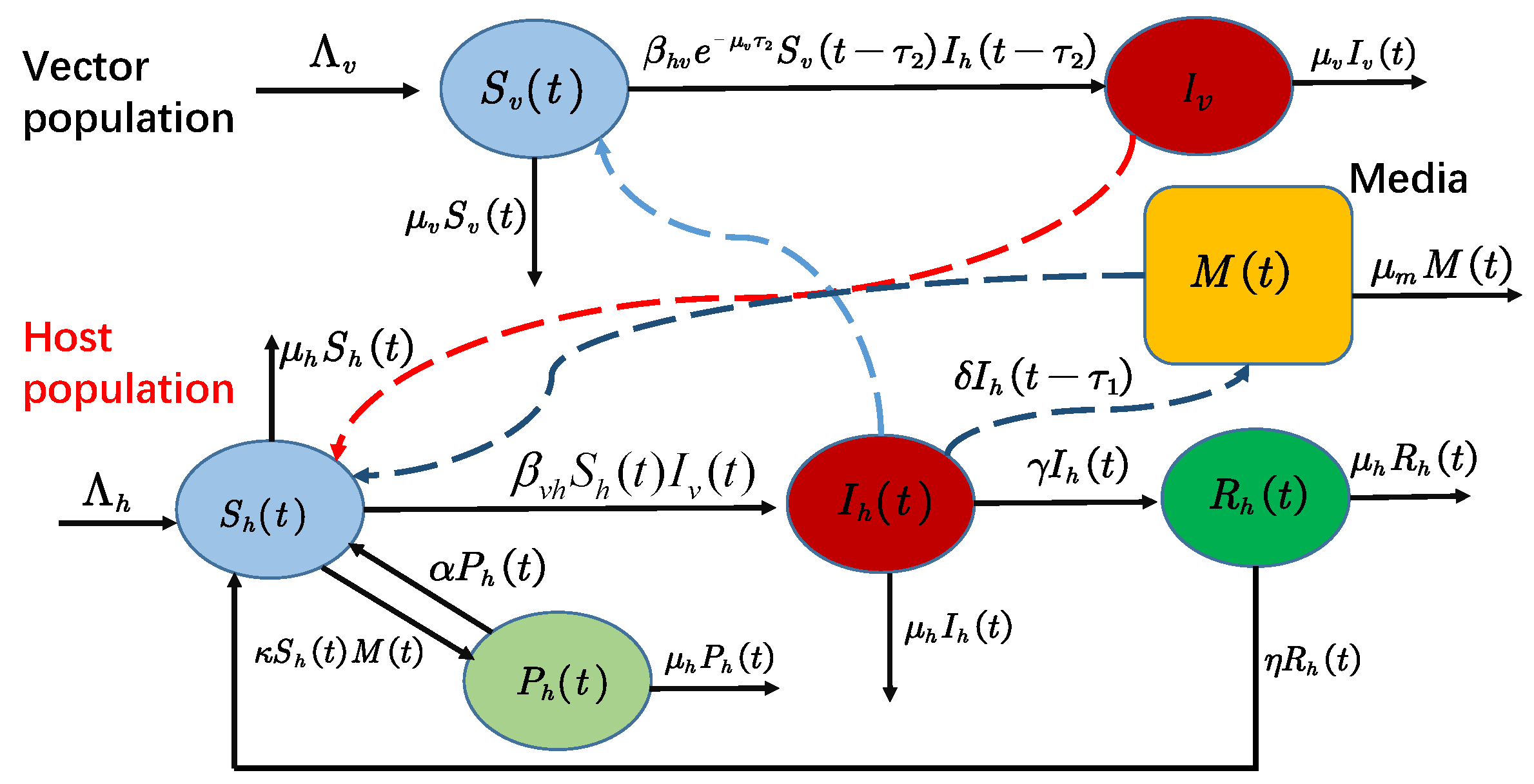In addition, delay ${\tau }_1$ is introduced to describe the delay between media reports and infectious disease screening and reporting of cases, and delay ${\tau }_2$ is given to describe the incubation period of the virus in vectors on disease transmission. Based on the classical vector-borne disease models (see [5,6,7,13,14,19,33] for more detail), the relationship between pathogens, hosts, vectors, and media coverage is shown in Figure 1. Based on the above assumption, a model reads as

$$\left\{\begin{array}{cc}\frac{\mathrm{d}{S}_h\left(t\right)}{\mathrm{d}t}=\hfill & {\mathrm{\Lambda }}_h-{\beta }_{vh}{S}_h\left(t\right)I_v\left(t\right)+\alpha P_h\left(t\right)-\kappa S_h\left(t\right)M\left(t\right)+\eta R_h\left(t\right)-{\mu }_h{S}_h\left(t\right),\hfill \\ \frac{\mathrm{d}{I}_h\left(t\right)}{\mathrm{d}t}=\hfill & {\beta }_{vh}{S}_h\left(t\right)I_v\left(t\right)-\gamma I_h\left(t\right)-{\mu }_h{I}_h\left(t\right),\hfill \\ \frac{\mathrm{d}{R}_h\left(t\right)}{\mathrm{d}t}=\hfill & \gamma I_h\left(t\right)-\eta R_h\left(t\right)-{\mu }_h{R}_h\left(t\right),\hfill \\ \frac{\mathrm{d}{P}_h\left(t\right)}{\mathrm{d}t}=\hfill & \kappa S_h\left(t\right)M\left(t\right)-\alpha P_h\left(t\right)-{\mu }_h{P}_h\left(t\right),\hfill \\ \frac{\mathrm{d}M\left(t\right)}{\mathrm{d}t}=\hfill & \delta I_h(t-{\tau }_1)-{\mu }_{m}M\left(t\right),\hfill \\ \frac{\mathrm{d}{S}_v\left(t\right)}{\mathrm{d}t}=\hfill & {\mathrm{\Lambda }}_v-{\beta }_{hv}{e}^{-{\mu }_v{\tau }_2}{S}_v(t-{\tau }_2)I_h(t-{\tau }_2)-{\mu }_v{S}_v\left(t\right),\hfill \\ \frac{\mathrm{d}{I}_v\left(t\right)}{\mathrm{d}t}=\hfill & {\beta }_{hv}{e}^{-{\mu }_v{\tau }_2}{S}_v(t-{\tau }_2)I_h(t-{\tau }_2)-{\mu }_v{I}_v\left(t\right).\hfill \end{array}\right.$$

(1)

The initial condition of Model (1) is

$$S_h\left(0\right)>0,I_h\left(\theta \right)={\varphi }_1\left(\theta \right),R_h\left(0\right)⩾0,P_h\left(0\right)⩾0,M\left(0\right)⩾0,S_v\left(\theta \right)={\varphi }_2\left(\theta \right),I_v\left(\theta \right)={\varphi }_3\left(\theta \right)$$

(2)

with ${\varphi }_i\left(\theta \right)$$(i=1,2,3)$ being non-negative continuous functions from $[-\tau ,0]$ to ${\mathbb{R}}_{+}^7:=\left\{(x_1,\cdots ,x_7)\right|x_i⩾0,i=1,\cdots ,7\}$ and $\tau =max\{{\tau }_1,{\tau }_2\}$.

The following Lemma 1 is on the existence of global positive solutions of Model (1), which is necessary for our discussion of its dynamics.

 Lemma 1. 

The solution $(S_h\left(t\right),I_h\left(t\right),R_h\left(t\right),P_h\left(t\right),M\left(t\right),S_v\left(t\right),S_v\left(t\right),I_v\left(t\right))$of Model (1) starting from the initial value (2) is existent, unique, and non-negative on $[0,\infty )$, which satisfies

$$\begin{array}{c}\hfill \underset{t\to \infty }{lim\; sup}N\left(t\right)⩽\frac{{\mathrm{\Lambda }}_h}{{\mu }_h},\underset{t\to \infty }{lim\; sup}{N}_v\left(t\right)⩽\frac{{\mathrm{\Lambda }}_v}{{\mu }_v},\underset{t\to \infty }{lim\; sup}M⩽\frac{\delta {\mathrm{\Lambda }}_h}{{\mu }_m{\mu }_h}.\end{array}$$

Further, if all initial values are positive, then the solution remains positive on $[0,\infty )$.

 Proof. 

Model (1) admits a unique solution $(S_h\left(t\right),I_h\left(t\right),R_h\left(t\right),P_h\left(t\right),M\left(t\right),S_v\left(t\right),I_v\left(t\right))$ with the initial condition (2) on $[0,T)$ by the basic theory of the functional differential equations [34], where $0<T⩽\infty$. Now, we verify, firstly, all components of the solution are positive on interval $[0,T)$, while all initial values are positive. If the conclusion is invalid, then there exists a positive constant $t^{*}\in (0,T)$ such that

$$\begin{array}{c}\hfill min\{S_h\left(t^{*}\right),I_h\left(t^{*}\right),R_h\left(t^{*}\right),P_h\left(t^{*}\right),M\left(t^{*}\right),S_v\left(t^{*}\right),I_v\left(t^{*}\right)\}=0\end{array}$$

and $S_h\left(t\right)>0$, $I_h\left(t\right)>0$, $R_h\left(t\right)>0$, $P_h\left(t\right)>0$, $M\left(t\right)>0$, $S_v\left(t\right)>0$, $I_v\left(t\right)>0$ for all $t\in [0,t^{*})$. Then, there are seven possible cases:$\left(i\right)$$S_h^{*}\left(t^{*}\right)=0$; $\left(ii\right)$$I_h\left(t^{*}\right)=0$; $R_h\left(t^{*}\right)=0$; $\left(iii\right)$$R_h\left(t^{*}\right)=0$; $\left(iv\right)$$P_h\left(t^{*}\right)=0$; $\left(v\right)$$M\left(t^{*}\right)=0$; $\left(vi\right)$$S_v\left(t^{*}\right)=0$ and $\left(vii\right)$$I_h\left(t^{*}\right)=0$. Now, we discuss only Cases $\left(i\right)$, $\left(ii\right)$, and $\left(v\right)$, the others are similar to these three.

 (i) 

If $S_h\left(t^{*}\right)=0$, then one has $\mathrm{d}{S}_h\left(t^{*}\right)/\mathrm{d}t⩽0$ due to $S\left(t\right)>0$ for $t\in [0,t^{*})$. However, from the S-equation of Model (1), it follows that

$$\begin{array}{c}\hfill \frac{\mathrm{d}{S}_h\left(t^{*}\right)}{\mathrm{d}t}=\mathrm{\Lambda }+\alpha P_h\left(t^{*}\right)+\eta R_h\left(t^{*}\right)⩾\mathrm{\Lambda }>0\end{array}$$

due to the fact that $R_h\left(t^{*}\right)⩾0$ and $P_h\left(t^{*}\right)⩾0$. This is a contradiction. Therefore, $S_h\left(t\right)>0$ for $t\in [0,T)$.

 (ii) 

If $I_h\left(t^{*}\right)=0$, this yields the $I_h$-equation of Model (1) that

$$\begin{array}{c}\hfill I_h\left(t^{*}\right)=\left(I_h\left(0\right)+{\int }_0^{t^{*}}{\beta }_{vh}{S}_h\left(t\right)I_v\left(t\right)e^{(\gamma +{\mu }_h)s}\mathrm{d}s\right)e^{-(\gamma +{\mu }_h)t^{*}}>0.\end{array}$$

This contradicts $I_h\left(t^{*}\right)=0$; that is, $I_h\left(t\right)>0$ for $t\in [0,T)$.

 (v) 

If $M\left(t^{*}\right)=0$, then one gets $\mathrm{d}M\left(t^{*}\right)/\mathrm{d}t⩽0$ due to $M\left(t\right)>0$ for $t\in [0,t^{*})$. However, from the M-equation, we can obtain

$$\begin{array}{c}\hfill \frac{\mathrm{d}M\left(t^{*}\right)}{\mathrm{d}t}=\delta I_h(t^{*}-{\tau }_1)-{\mu }_{m}M\left(t^{*}\right)=\delta I_h(t^{*}-{\tau }_1)>0\end{array}$$

due to $I_h\left(\theta \right)>0$ for $\theta \in [-\tau ,T)$. This also contradicts $M\left(t^{*}\right)=0$. Thus, $M\left(t\right)>0$ for $t\in [0,T)$.

To sum up the above discussion, we can find that all components of the solution are positive on interval $[0,T)$, while all initial values are positive. Further, from the continuous dependence of the solution on the initial value, we can see that the solution $(S_h\left(t\right)$, $I_h\left(t\right)$, $R_h\left(t\right)$, $P_h\left(t\right)$, $M\left(t\right)$, $S_v\left(t\right)$, $I_v\left(t\right))$ of Model (1) starting from the initial value (2) is existent, unique, and non-negative on $[0,T)$.

Finally, we focus on the global existence of solutions of Model (1). Adding the hosts equations and the last two equations of Model (1), respectively, one has

$$\begin{array}{c}\hfill \frac{\mathrm{d}{N}_h\left(t\right)}{\mathrm{d}t}={\mathrm{\Lambda }}_h-{\mu }_h{N}_h\left(t\right),\frac{\mathrm{d}{N}_v\left(t\right)}{\mathrm{d}t}={\mathrm{\Lambda }}_v-{\mu }_v{N}_v\left(t\right).\end{array}$$

Then, $N_h\left(t\right)$ and $N_v\left(t\right)$ are bounded in $t\in [0,T)$, and the bounds can be chosen to be ${\tilde{N}}_h^0=max\{N_h\left(0\right),{\mathrm{\Lambda }}_h/{\mu }_h\}$ and ${\tilde{N}}_v^0=max\{N_v\left(0\right),{\mathrm{\Lambda }}_v/{\mu }_v\}$. Further, it yields from the M-equation that $\mathrm{d}M\left(t\right)/\mathrm{d}t⩽\delta {\tilde{N}}_h^0-{\mu }_{m}M$. This implies that $M\left(t\right)$ is bound in interval $[0,T)$. Thus, again, utilizing the basic theory of functional differential equations, the solution $(S_h\left(t\right),I_h\left(t\right),R_h\left(t\right),P_h\left(t\right),M\left(t\right),S_v\left(t\right),I_v\left(t\right))$ is existent, unique, non-negative, and bounded on $[0,\infty )$. The proof is finished. □

According to the limit theory of dynamical systems [35], the dynamics of Model (1) are equivalent to the following model:

$$\left\{\begin{array}{cc}\frac{\mathrm{d}{S}_h\left(t\right)}{\mathrm{d}t}=\hfill & {\mathrm{\Lambda }}_h-{\beta }_{vh}{S}_h\left(t\right)I_v\left(t\right)+\alpha \left(\frac{{\mathrm{\Lambda }}_h}{{\mu }_h}-S_h\left(t\right)-I_h\left(t\right)-R_h\left(t\right)\right)\hfill \\ \hfill & -\kappa S_h\left(t\right)M\left(t\right)+\eta R_h\left(t\right)-{\mu }_h{S}_h\left(t\right),\hfill \\ \frac{\mathrm{d}{I}_h\left(t\right)}{\mathrm{d}t}=\hfill & {\beta }_{vh}{S}_h\left(t\right)I_v\left(t\right)-\gamma I_h\left(t\right)-{\mu }_h{I}_h\left(t\right),\hfill \\ \frac{\mathrm{d}{R}_h\left(t\right)}{\mathrm{d}t}=\hfill & \gamma I_h\left(t\right)-\eta R_h\left(t\right)-{\mu }_h{R}_h\left(t\right),\hfill \\ \frac{\mathrm{d}M\left(t\right)}{\mathrm{d}t}=\hfill & \delta I_h(t-{\tau }_1)-{\mu }_{m}M\left(t\right),\hfill \\ \frac{\mathrm{d}{I}_v\left(t\right)}{\mathrm{d}t}=\hfill & {\beta }_{hv}{e}^{-{\mu }_v{\tau }_2}\left(\frac{{\mathrm{\Lambda }}_v}{{\mu }_v}-I_v(t-{\tau }_2)\right)I_h(t-{\tau }_2)-{\mu }_v{I}_v\left(t\right).\hfill \end{array}\right.$$

(3)

From the proof of Lemma 1, $\mathrm{\Omega }$ is a positively invariant, where

$$\begin{array}{c}\hfill \mathrm{\Omega }=\left\{(S_h,I_h,R_h,M,I_v)\in {\mathbb{R}}_{+}^{5}0\le S_h,I_h,R_h\le \frac{{\mathrm{\Lambda }}_h}{{\mu }_h},0\le M\le \frac{\delta {\mathrm{\Lambda }}_h}{{\mu }_m{\mu }_h},0\le I_v\le \frac{{\mathrm{\Lambda }}_v}{{\mu }_v}\right\}.\end{array}$$

Therefore, in the rest of this paper, we study the dynamics of Model (3) on $\mathrm{\Omega }$.

3. Stability of Disease-Free Equilibrium

It is obvious that Model (3) admits the disease-free equilibrium ${\mathcal{E}}_0=({\mathrm{\Lambda }}_h/{\mu }_h,0,0,0,0)$. Define the basic reproduction number as

$$\begin{array}{c}\hfill {\mathcal{R}}_0=\sqrt{\frac{e^{-{\mu }_v{\tau }_2}{\beta }_{vh}{\beta }_{hv}{\mathrm{\Lambda }}_h{\mathrm{\Lambda }}_v}{{\mu }_h{\mu }_v^2(\gamma +{\mu }_h)}}.\end{array}$$

Further, the endemic equilibrium ${\mathcal{E}}^{*}=(S_h^{*},I_h^{*},R_h^{*},M^{*},I_v^{*})$ of (3) satisfies

$$\left\{\begin{array}{cc}\hfill 0=& {\mathrm{\Lambda }}_h-{\beta }_{vh}{S}_h^{*}{I}_v^{*}+\alpha \frac{{\mathrm{\Lambda }}_h}{{\mu }_h}-\alpha S_h^{*}-\alpha I_h^{*}-\alpha R_h^{*}-\kappa S_h^{*}{M}^{*}+\eta R_h^{*}-{\mu }_h{S}_h^{*},\hfill \\ \hfill 0=& {\beta }_{vh}{S}_h^{*}{I}_v^{*}-\gamma I_h^{*}-{\mu }_h{I}_h^{*},\hfill \\ \hfill 0=& \gamma I_h^{*}-\eta R_h^{*}-{\mu }_h{R}_h^{*},\hfill \\ \hfill 0=& \delta I_h^{*}-{\mu }_m{M}^{*},\hfill \\ \hfill 0=& {\beta }_{hv}{e}^{-{\mu }_v{\tau }_2}\left(\frac{{\mathrm{\Lambda }}_v}{{\mu }_v}-I_v^{*}\right)I_h^{*}-{\mu }_v{I}_v^{*}.\hfill \end{array}\right.$$

By direct calculation,

$$\begin{array}{cc}\hfill & S_h^{*}=\frac{{\mu }_v({\beta }_{hv}{e}^{-{\mu }_v{\tau }_2}{I}_h^{*}+{\mu }_v)[({\mathrm{\Lambda }}_h+\alpha \frac{{\mathrm{\Lambda }}_h}{{\mu }_h}-\alpha I_h^{*})(\eta +{\mu }_h)+\gamma (\eta -\alpha )I_h^{*}]}{(\eta +{\mu }_h)[{\beta }_{vh}{\beta }_{hv}{e}^{-{\mu }_v{\tau }_2}{\mathrm{\Lambda }}_v{I}_h^{*}+{\mu }_v(\alpha +\kappa \frac{\delta }{{\mu }_m}{I}_h^{*}+{\mu }_h)({\beta }_{hv}{e}^{-{\mu }_v{\tau }_2}{I}_h^{*}+{\mu }_v)]}\hfill \\ \hfill & I_h^{*}=\frac{{\beta }_{vh}{S}_h^{*}{I}_v^{*}}{\gamma +{\mu }_h},R_h^{*}=\frac{\gamma }{\eta +{\mu }_h}{I}_h^{*},I_v^{*}=\frac{{\beta }_{hv}{e}^{-{\mu }_v{\tau }_2}{\mathrm{\Lambda }}_v}{{\mu }_v({\beta }_{hv}{e}^{-{\mu }_v{\tau }_2}{I}_h^{*}+{\mu }_v)}{I}_h^{*},M^{*}=\frac{\delta }{{\mu }_m}{I}_h^{*},\hfill \end{array}$$

where $I_h^{*}$ is the positive root of the quadratic equation

$$C_1{I_h^{*}}^2+C_2{I}_h^{*}+C_3=0,$$

(4)

where

$$\begin{array}{cc}\hfill C_1=& {\mu }_v\kappa {\beta }_{hv}{e}^{-{\mu }_v{\tau }_2}\frac{\delta }{{\mu }_m}(\gamma +{\mu }_h)(\eta +{\mu }_h),\hfill \\ \hfill C_2=& {\mu }_v(\eta +{\mu }_h)(\gamma +{\mu }_h)(\alpha +{\mu }_h){\beta }_{hv}{e}^{-{\mu }_v{\tau }_2}+\kappa {\mu }_v^2(\eta +{\mu }_h)(\gamma +{\mu }_h)\frac{\delta }{{\mu }_m}\hfill \\ \hfill & +{\mathrm{\Lambda }}_v{\beta }_{vh}{\beta }_{hv}{e}^{-{\mu }_v{\tau }_2}\left[{\mu }_h^2+(\alpha +\eta +\gamma ){\mu }_h+\alpha (\gamma +\eta )\right],\hfill \\ \hfill C_3=& {\mu }_v^2(\alpha +{\mu }_h)(\gamma +{\mu }_h)(\eta +{\mu }_h)(1-{\mathcal{R}}_0^2).\hfill \end{array}$$

Let

$$\begin{array}{c}\hfill I_{h_1}^{*}=\frac{-C_2+\sqrt{C_2^2-4C_1{C}_3}}{2C_1},I_{h_2}^{*}=\frac{-C_2-\sqrt{C_2^2-4C_1{C}_3}}{2C_1}\end{array}$$

be two roots of (4). From the expressions, we have that $C_1>0$, $C_2>0$. Further, $C_3>0$ if ${\mathcal{R}}_0<1$, and $C_3<0$ if ${\mathcal{R}}_0>1$. It is easy to see that $I_1^{*}$ and $I_2^{*}$ are negative if ${\mathcal{R}}_0<1$, and $I_1^{*}$ is positive and $I_2^{*}$ is negative if ${\mathcal{R}}_0>1$. From the relationship between the roots of Equation (4) and the equilibrium of Model (3), the following result is valid.

 Theorem 1. 

There is always the disease-free equilibrium ${\mathcal{E}}_0$to Model (3); however, if ${\mathcal{R}}_0>1$, Model (3) admits a unique endemic equilibrium ${\mathcal{E}}^{*}$ in addition to ${\mathcal{E}}_0$.

In order to investigate the local stability of any equilibrium $\tilde{\mathcal{E}}=({\tilde{S}}_h,{\tilde{I}}_h,{\tilde{R}}_h,\tilde{M},{\tilde{I}}_v)$ of Model (3), we linearize this model and obtain the characteristic equation at $\tilde{\mathcal{E}}$ as

$$|\lambda E-J(\tilde{\mathcal{E}}\left)\right|=0,$$

where

$$\begin{array}{ccc}\hfill & J\left(\tilde{\mathcal{E}}\right)=\hfill & \hfill \left(\begin{array}{ccccc}-{\beta }_{vh}{\tilde{I}}_v-\alpha -\kappa \tilde{M}-{\mu }_h& -\alpha & -\alpha +\eta & -\kappa {\tilde{S}}_h& -{\beta }_{vh}{\tilde{S}}_h\\ {\beta }_{vh}{\tilde{I}}_v& -\gamma -{\mu }_h& 0& 0& {\beta }_{vh}{\tilde{S}}_h\\ 0& \gamma & -\eta -{\mu }_h& 0& 0\\ 0& \delta e^{-\lambda {\tau }_1}& 0& -{\mu }_m& 0\\ 0& {\beta }_{hv}{e}^{-({\mu }_v+\lambda ){\tau }_2}(\frac{{\mathrm{\Lambda }}_v}{{\mu }_v}-{\tilde{I}}_v)& 0& 0& -{\beta }_{hv}{e}^{-({\mu }_v+\lambda ){\tau }_2}{\tilde{I}}_h-{\mu }_v\end{array}\right).\end{array}$$

(5)

It is clear that the characteristic equation at ${\mathcal{E}}_0=({\mathrm{\Lambda }}_h/{\mu }_h,0,0,0,0)$ becomes

$$(\lambda +\alpha +{\mu }_h)(\lambda +\eta +{\mu }_h)(\lambda +{\mu }_m)[F\left(\lambda \right)-G\left(\lambda \right)]=0,$$

(6)

where $F\left(\lambda \right)={\lambda }^2+(\gamma +{\mu }_h+{\mu }_v)\lambda +(\gamma +{\mu }_h){\mu }_v,G\left(\lambda \right)={\beta }_{hv}{\beta }_{vh}({\mathrm{\Lambda }}_h{\mathrm{\Lambda }}_v/{\mu }_h{\mu }_v)e^{-({\mu }_v+\lambda ){\tau }_2}$. Note that three roots of (6) are ${\lambda }_1=-(\alpha +{\mu }_h)<0$, ${\lambda }_2=-(\eta +{\mu }_h)<0$, ${\lambda }_3=-{\mu }_m<0$. So, the stability of ${\mathcal{E}}_0$ is given by the real part of roots of the following equation

$$F\left(\lambda \right)-G\left(\lambda \right)={\lambda }^2+(\gamma +{\mu }_h+{\mu }_v)\lambda +(\gamma +{\mu }_h){\mu }_v-\frac{{\beta }_{hv}{\beta }_{vh}{\mathrm{\Lambda }}_h{\mathrm{\Lambda }}_v}{{\mu }_h{\mu }_v}{e}^{-({\mu }_v+\lambda ){\tau }_2}=0.$$

(7)

Obviously,

$$\begin{array}{c}\hfill (\gamma +{\mu }_h){\mu }_v-\frac{{\beta }_{hv}{\beta }_{vh}{\mathrm{\Lambda }}_h{\mathrm{\Lambda }}_v}{{\mu }_h{\mu }_v}{e}^{-({\mu }_v+\lambda ){\tau }_2}=(\gamma +{\mu }_h){\mu }_v\left(1-{\mathcal{R}}_0^2{e}^{-\lambda {\tau }_2}\right),\end{array}$$

and (7) reads as, for ${\tau }_2=0$,

$${\lambda }^2+(\gamma +{\mu }_h+{\mu }_v)\lambda +(\gamma +{\mu }_h){\mu }_v\left(1-{\mathcal{R}}_0^2\right)=0.$$

(8)

The roots of (8) have negative real parts if ${\mathcal{R}}_0<1$. Further, since the roots of (7) depend on ${\tau }_2$ continuously (see for [36] more details), then the real part of the root only becomes positive by crossing through the imaginary axis in the complex plane. Note that $\lambda =0$ is not a root, amd the roots of (7) can cross the imaginary axis, that is, $\lambda =i\omega (\omega >0)$. Now, substituting $\lambda =i\omega$ into (8) and separating the real and imaginary parts, one has

$$\begin{array}{cc}\hfill -{\omega }^2+(\gamma +{\mu }_h){\mu }_v=& {\beta }_{hv}{\beta }_{vh}\frac{{\mathrm{\Lambda }}_h{\mathrm{\Lambda }}_v}{{\mu }_h{\mu }_v}{e}^{-{\mu }_v{\tau }_2}cos\left(\omega {\tau }_2\right),\hfill \\ \hfill (\gamma +{\mu }_v+{\mu }_h)\omega =& -{\beta }_{hv}{\beta }_{vh}\frac{{\mathrm{\Lambda }}_h{\mathrm{\Lambda }}_v}{{\mu }_h{\mu }_v}{e}^{-{\mu }_v{\tau }_2}sin\left(\omega {\tau }_2\right).\hfill \end{array}$$

Squaring and taking the sum of the above two equations, one can easily obtain

$${\omega }^4+[{\mu }_v^2+{(\gamma +{\mu }_h)}^2]{\omega }^2+{\mu }_v^2{(\gamma +{\mu }_h)}^2\left(1-{\mathcal{R}}_0^4\right)=0.$$

(9)

From Expression (9), it is found that the equation has no positive roots for ${\mathcal{R}}_0<1$. Therefore, all of the roots of (7) are in the left-half plane for all ${\tau }_2>0$ if ${\mathcal{R}}_0<1$. That is, the disease-free equilibrium ${\mathcal{E}}_0$ of Model (3) is local asymptotically stable for this case. However, for ${\mathcal{R}}_0>1$, Equation (9) has a positive root, which implies ${\mathcal{E}}_0$ is unstable. By the above discussion, the following result is valid.

 Theorem 2. 

The disease-free equilibrium ${\mathcal{E}}_0$ of Model (3) is locally asymptotically stable if ${\mathcal{R}}_0<1$, and which is unstable for ${\mathcal{R}}_0>1$.

4. Stability of the Endemic Equilibrium and Bifurcatioan Analysis

From (5), the characteristic equation of Model (3) at ${\mathcal{E}}^{*}=(S_h^{*},I_h^{*},R_h^{*},M^{*},I_v^{*})$ reads as

$$\begin{array}{cc}\hfill & {\lambda }^5+A_1{\lambda }^4+A_2{\lambda }^3+A_3{\lambda }^2+A_4\lambda +A_5+e^{-\lambda {\tau }_2}(B_1{\lambda }^4+B_2{\lambda }^3+B_3{\lambda }^2+B_4\lambda +B_5)\hfill \\ \hfill & +e^{-\lambda {\tau }_1}(D_1{\lambda }^2+D_2\lambda +D_3)+e^{-\lambda ({\tau }_1+{\tau }_2)}(E_1\lambda +E_2)=0,\hfill \end{array}$$

(10)

where $B_1={\beta }_{hv}{I}_h^{*}{e}^{-{\mu }_v{\tau }_2}$, and

$$\begin{array}{cc}\hfill B_2=& {\beta }_{hv}{I}_h^{*}{e}^{-{\mu }_v{\tau }_2}(\eta +\gamma +2{\mu }_h+{\mu }_m+\alpha +{\mu }_h+\kappa M^{*}+{\beta }_{vh}{I}_v^{*})-{\beta }_{vh}{\beta }_{hv}{e}^{-{\mu }_v{\tau }_2}{S}_h^{*}\left(\frac{{\mathrm{\Lambda }}_v}{{\mu }_v}-I_v^{*}\right),\hfill \\ \hfill B_3=& \alpha {\beta }_{hv}{\beta }_{hv}{I}_h^{*}{I}_v^{*}{e}^{-{\mu }_v{\tau }_2}-{\beta }_{vh}{\beta }_{hv}{S}_h^{*}{e}^{-{\mu }_v{\tau }_2}\left(\frac{{\mathrm{\Lambda }}_v}{{\mu }_v}-I_v^{*}\right)(\eta +{\mu }_h+{\mu }_m+\alpha +{\mu }_h+\kappa M^{*}+{\beta }_{vh}{I}_v^{*})\hfill \\ \hfill & +{\beta }_{hv}{I}_h^{*}{e}^{-{\mu }_v{\tau }_2}[(\eta +{\mu }_h+{\mu }_m)(\gamma +{\mu }_h)+{\mu }_m(\eta +{\mu }_h)]+{\beta }_{vh}^2{\beta }_{hv}{e}^{-{\mu }_v{\tau }_2}{I}_v^{*}{S}_h^{*}\left(\frac{{\mathrm{\Lambda }}_v}{{\mu }_v}-I_v^{*}\right)\hfill \\ \hfill & +{\beta }_{hv}{I}_h^{*}{e}^{-{\mu }_v{\tau }_2}(\alpha +{\mu }_h+\kappa M^{*}+{\beta }_{vh}{I}_v^{*})(\eta +\gamma +2{\mu }_h+{\mu }_m),\hfill \\ \hfill B_4=& {\beta }_{vh}^2{\beta }_{hv}{e}^{-{\mu }_v{\tau }_2}{I}_v^{*}{S}_h^{*}\left(\frac{{\mathrm{\Lambda }}_v}{{\mu }_v}-I_v^{*}\right)(\eta +{\mu }_h+{\mu }_m)+{\beta }_{hv}{\beta }_{hv}{I}_h^{*}{I}_v^{*}{e}^{-{\mu }_v{\tau }_2}[\alpha (\eta +{\mu }_h+{\mu }_v)+\gamma (\alpha -\eta )]\hfill \\ \hfill & +{\beta }_{hv}{I}_h^{*}{e}^{-{\mu }_v{\tau }_2}[(\alpha +{\mu }_h+\kappa M^{*}+{\beta }_{vh}{I}_v^{*})(\eta +{\mu }_h+{\mu }_m)(\gamma +{\mu }_h)+{\mu }_m(\eta +{\mu }_h)(\gamma +{\mu }_h)]\hfill \\ \hfill & -{\beta }_{hv}{\beta }_{vh}{S}_h^{*}{e}^{-{\mu }_v{\tau }_2}\left(\frac{{\mathrm{\Lambda }}_v}{{\mu }_v}-I_v^{*}\right)[(\alpha +{\mu }_h+\kappa M^{*}+{\beta }_{vh}{I}_v^{*})(\eta +{\mu }_h+{\mu }_m)+{\mu }_m(\eta +{\mu }_h)],\hfill \\ \hfill B_5=& {\mu }_m{\beta }_{vh}^2{\beta }_{hv}{e}^{-{\mu }_v{\tau }_2}{I}_v^{*}{S}_h^{*}\left(\frac{{\mathrm{\Lambda }}_v}{{\mu }_v}-I_v^{*}\right)(\eta +{\mu }_h)+{\beta }_{hv}{\beta }_{hv}{I}_h^{*}{I}_v^{*}{e}^{-{\mu }_v{\tau }_2}[\alpha {\mu }_m(\eta +{\mu }_h)+\gamma {\mu }_m(\alpha -\eta )]\hfill \\ \hfill & +{\mu }_m{\beta }_{hv}{I}_h^{*}{e}^{-{\mu }_v{\tau }_2}(\alpha +{\mu }_h+\kappa M^{*}+{\beta }_{vh}{I}_v^{*})(\eta +{\mu }_h)(\gamma +{\mu }_h)\hfill \\ \hfill & -{\mu }_m{\beta }_{hv}{\beta }_{vh}{S}_h^{*}{e}^{-{\mu }_v{\tau }_2}\left(\frac{{\mathrm{\Lambda }}_v}{{\mu }_v}-I_v^{*}\right)(\alpha +{\mu }_h+\kappa M^{*}+{\beta }_{vh}{I}_v^{*})(\eta +{\mu }_h),\hfill \\ \hfill A_1=& \gamma +\eta +3{\mu }_h+{\mu }_v+{\mu }_m+\alpha +\kappa M^{*}+{\beta }_{vh}{I}_v^{*},\hfill \\ \hfill A_2=& {\mu }_v(\gamma +{\mu }_h)+{\mu }_m(\eta +{\mu }_h)+(\alpha +{\mu }_h+\kappa M^{*}+{\beta }_{vh}{I}_v^{*})(\gamma +\eta +2{\mu }_h+{\mu }_v+{\mu }_m)\hfill \\ \hfill & +(\eta +{\mu }_h+{\mu }_m)(\gamma +{\mu }_h+{\mu }_v)+\alpha {\beta }_{vh}{I}_v^{*},\hfill \\ \hfill A_3=& (\alpha +{\mu }_h+\kappa M^{*}+{\beta }_{vh}{I}_v^{*})[{\mu }_v(\gamma +{\mu }_h)+{\mu }_m(\eta +{\mu }_h)+(\eta +{\mu }_h+{\mu }_m)(\gamma +{\mu }_h+{\mu }_v)]\hfill \\ \hfill & +{\mu }_v(\gamma +{\mu }_h)(\eta +{\mu }_h+{\mu }_m)+{\mu }_m(\eta +{\mu }_h)(\gamma +{\mu }_h+{\mu }_v)\hfill \\ \hfill & +{\beta }_{vh}{I}_v^{*}[\alpha {\mu }_v+\alpha (\eta +{\mu }_h+{\mu }_m)+\gamma (\alpha -\eta )],\hfill \\ \hfill A_4=& (\alpha +{\mu }_h+\kappa M^{*}+{\beta }_{vh}{I}_v^{*})[{\mu }_v(\gamma +{\mu }_h)(\eta +{\mu }_h+{\mu }_m)+{\mu }_m(\eta +{\mu }_h)(\gamma +{\mu }_h+{\mu }_v)]\hfill \\ \hfill & +{\beta }_{vh}{I}_v^{*}[\alpha {\mu }_m(\eta +{\mu }_h)+\gamma {\mu }_m(\alpha -\eta )+{\mu }_v\alpha (\eta +{\mu }_h+{\mu }_m)+{\mu }_v\gamma (\alpha -\eta )]\hfill \\ \hfill & +{\mu }_m{\mu }_v(\eta +{\mu }_h)(\gamma +{\mu }_h),\hfill \\ \hfill A_5=& {\mu }_m{\mu }_v(\alpha +{\mu }_h+\kappa M^{*}+{\beta }_{vh}{I}_v^{*})(\eta +{\mu }_h)(\gamma +{\mu }_h)+{\mu }_v{\beta }_{vh}{I}_v^{*}[\alpha {\mu }_m(\eta +{\mu }_h)+\gamma {\mu }_m(\alpha -\eta )],\hfill \\ \hfill D_1=& \delta \kappa {\beta }_{vh}{I}_v^{*}{S}_h^{*},D_2=\delta \kappa {\beta }_{vh}{I}_v^{*}{S}_h^{*}(\eta +{\mu }_h+{\mu }_v),D_3={\mu }_v\delta \kappa {\beta }_{vh}{I}_v^{*}{S}_h^{*}(\eta +{\mu }_h),\hfill \\ \hfill E_1=& \delta \kappa {\beta }_{hv}{\beta }_{vh}{I}_v^{*}{I}_h^{*}{S}_h^{*}{e}^{-{\mu }_v{\tau }_2},E_2=\delta \kappa {\beta }_{hv}{\beta }_{vh}{I}_v^{*}{I}_h^{*}{S}_h^{*}{e}^{-{\mu }_v{\tau }_2}(\eta +{\mu }_h).\hfill \end{array}$$

Here, for the two different delays ${\tau }_1$ and ${\tau }_2$, the stability of the endemic equilibrium ${\mathcal{E}}^{*}$ can be categorized as follows: $\left(\mathrm{i}\right)$${\tau }_1={\tau }_2=0$; $\left(\mathrm{ii}\right)$${\tau }_1=0$ and ${\tau }_2>0$; $\left(\mathrm{iii}\right)$${\tau }_1>0$ and ${\tau }_2=0$; $\left(\mathrm{iv}\right)$${\tau }_1\in (0,{\tau }_1^0)$ and ${\tau }_2>0$; $\left(\mathrm{v}\right)$${\tau }_1>0$ and ${\tau }_2\in (0,{\tau }_2^0)$.

• Case (i) ${\tau }_1={\tau }_2=0$.

From the Jacobian matrix (5) in this case, the characteristic Equation (10) is equivalent to

$${\lambda }^5+K_1{\lambda }^4+K_2{\lambda }^3+K_3{\lambda }^2+K_4\lambda +K_5=0$$

(11)

with $K_i=A_i+B_i(i=1,2),K_3=A_3+B_3+D_1,K_4=A_4+B_4+D_2+E_1,K_5=A_5+B_5+D_3+E_2.$ Obviously, $K_1>0$ and $K_5>0$. As the application of Routh–Hurwitz criteria, if

$$\begin{array}{cc}\hfill & H_2=K_1{K}_2-K_3>0,H_3=K_3{H}_2-K_1^2{K}_4+K_1{K}_5>0,\hfill \\ & H_4=K_4{H}_3-K_2{K}_5{H}_2-K_5^2+K_1{K}_4{K}_5>0,\hfill \end{array}$$

(12)

then all roots of (11) have negative real parts; that is, the endemic equilibrium ${\mathcal{E}}^{*}$ is locally asymptotically stable.

Summarizing the above discussion, Theorem 3 is obvious.

 Theorem 3. 

If ${\mathcal{R}}_0>1$ and (12) hold, the endemic equilibrium ${\mathcal{E}}^{*}$ of Model (3) is locally asymptotically stable.

• Case (ii) ${\tau }_1=0$, ${\tau }_2>0$

If ${\tau }_1=0$ and ${\tau }_2>0$, it yields from (5) that the characteristic Equation (10) is

$$\begin{array}{cc}\hfill & {\lambda }^5+A_1{\lambda }^4+A_2{\lambda }^3+(A_4+D_2)\lambda +(A_5+D_3)\hfill \\ \hfill & +[B_1{\lambda }^4+B_2{\lambda }^3+B_3{\lambda }^2+(B_4+E_1)\lambda +e^{-\lambda {\tau }_2}(B_5+E_2)]=0.\hfill \end{array}$$

(13)

Suppose $\lambda =i\omega$$(\omega >0)$ is a root of Equation (13), then this separates the real and imaginary parts such that

$$\begin{array}{cc}\hfill & (B_1{\omega }^4-B_3{\omega }^2+B_5+E_2)cos\left(\omega {\tau }_2\right)+[B_2{\omega }^3(B_4+E_1)\omega -B_2{\omega }^3]sin\left(\omega {\tau }_2\right)\hfill \\ \hfill =& (A_3+D_1){\omega }^2-A_1{\omega }^4-(A_5+D_3)\hfill \end{array}$$

(14)

and

$$\begin{array}{cc}\hfill & -(B_1{\omega }^4-B_3{\omega }^2+B_5+E_2)sin\left(\omega {\tau }_2\right)+[(B_4+E_1)\omega -B_2{\omega }^3]cos\left(\omega {\tau }_2\right)\hfill \\ \hfill =& A_2{\omega }^3-{\omega }^5-(A_4+D_2)\omega .\hfill \end{array}$$

(15)

Squaring and adding both (14) and (15) leads to the following equation:

$${\omega }^{10}+T_1{\omega }^8+T_2{\omega }^6+T_3{\omega }^4+T_4{\omega }^2+T_5=0,$$

(16)

where

$$\begin{array}{cc}\hfill T_1=& A_1^2-B_1^2-2A_2,T_5={(A_5+D_3)}^2-{(B_5+E_2)}^2,\hfill \\ \hfill T_2=& A_2^2-B_2^2+2(A_4+D_2)-2A_1(A_3+D_1)+2B_1{B}_3,\hfill \\ \hfill T_4=& {(A_4+D_2)}^2-2(A_3+D_1)(A_5+D_3)-{(B_4+E_1)}^2+2(B_3{B}_5+B_3{E}_2),\hfill \\ \hfill T_3=& -B_3^2-2B_1{B}_5-2B_1{E}_2+2B_2(B_4+E_1)+{(A_3+D_1)}^2+2A_1(A_5+D_3)-2A_2(A_4+D_2).\hfill \end{array}$$

(17)

Set ${\omega }^2=\xi$ in Equation (16), then we obtain

$$\begin{array}{c}\hfill H\left(\xi \right):={\xi }^5+T_1{\xi }^4+T_2{\xi }^3+T_3{\xi }^2+T_4\xi +T_5=0.\end{array}$$

(18)

If ${(A_5+D_3)}^2<{(B_5+E_2)}^2$, then $H\left(0\right)=T_5<0$ and $H(\infty )=\infty$, Equation (18) has at least one positive root.

 Theorem 4. 

Suppose that the conditions of Theorem 3 hold and ${\tau }_1=0$. If ${(A_5+D_3)}^2<{(B_5+E_2)}^2$, then the endemic equilibrium ${\mathcal{E}}^{*}$ of Model (3) is asymptotically stable for $0<{\tau }_2<{\tau }_2^0$. Furthermore, if $\mathrm{d}H\left(\xi \right)/\mathrm{d}\xi >0$ for $\xi >0$, then Model (3) undergoes the Hopf bifurcation for ${\tau }_2={\tau }_2^0$, where

$$\begin{array}{c}\hfill {\tau }_2^0={\frac{1}{\omega }}_{2_0}arctan\left(\frac{L_1}{L_2}\right),\end{array}$$

${\omega }_{2_0}$ is the positive root of Equation (13) and

$$\begin{array}{cc}\hfill L_1=& (B_1{\omega }^4-B_3{\omega }^2+B_5+E_2)[A_2{\omega }^3-{\omega }^5-(A_4+D_2)\omega ]\hfill \\ \hfill & +[B_2{\omega }^3-(B_4+E_1)\omega ][(A_3+D_1){\omega }^2-A_1{\omega }^4-(A_5+D_3)],\hfill \\ \hfill L_2=& (B_1{\omega }^4-B_3{\omega }^2+B_5+E_2)[(A_3+D_1){\omega }^2-A_1{\omega }^4-(A_5+D_3)]\hfill \\ \hfill & -[B_2{\omega }^3-(B_4+E_1)\omega ][A_2{\omega }^3-{\omega }^5-(A_4+D_2)\omega ].\hfill \end{array}$$

(19)

 Proof. 

If ${(A_5+D_3)}^2<{(B_5+E_2)}^2$, then Equation (18) has at least one positive root ${\xi }_0$. So, Equation (16) admits a positive root ${\omega }_{2_0}$. Then, the characteristic Equation (13) has a pair of pure imaginary roots $\pm i{\omega }_{2_0}$. Further, from Equations (14) and (15), ${\tau }_{2_k}^0(k=0,1,2,\cdots )$ is a function of ${\omega }_{2_0}$, and

$${\tau }_{2_k}^0=\frac{1}{{\omega }_{2_0}}arctan\left(\frac{L_1}{L_2}\right)+\frac{k\pi }{{\omega }_{2_0}}.$$

Define ${\tau }_2^0={min}_{k\ge 0}\left\{{\tau }_{2_k}^0\right\}$. If the conditions of Theorem 3 hold and ${\tau }_2<{\tau }_2^0$, ${\mathcal{E}}^{*}$ keeps its stability from the Butler Lemma (see [37] for more details). In the following, we verify the transversality condition $sign{\left\{\mathrm{d}Re\left(\lambda {\tau }_2\right)/\mathrm{d}{\tau }_2\right\}}_{{\tau }_2={\tau }_2^0}$. Differentiating Equation (13), we obtain

$$\begin{array}{c}\hfill {\left(\frac{\mathrm{d}\lambda }{\mathrm{d}{\tau }_2}\right)}^{-1}=\frac{m_1}{\lambda G\left(\lambda \right)}+\frac{m_2}{\lambda m_3}-\frac{{\tau }_2}{\lambda }\end{array}$$

with

$$\begin{array}{cc}\hfill m_1& =5{\lambda }^4+4A_1{\lambda }^3+3A_2{\lambda }^2+2(A_3+D_1)\lambda +(A_4+D_2),\hfill \\ \hfill m_2& =4B_1{\lambda }^3+3B_2{\lambda }^2+2B_3\lambda +(B_4+E_1),\hfill \\ \hfill m_3& =B_1{\lambda }^4+B_2{\lambda }^3+B_3{\lambda }^2+(B_4+E_1)\lambda +(B_5+E_2),\hfill \\ \hfill G\left(\lambda \right)& =e^{\lambda {\tau }_2}[B_1{\lambda }^4+B_2{\lambda }^3+B_3{\lambda }^2+(B_4+E_1)\lambda +(B_5+E_2)].\hfill \end{array}$$

From (13) and (16), it yields that

$$\begin{array}{cc}\hfill & sign{\left\{\frac{\mathrm{d}Re\left(\lambda \left({\tau }_2\right)\right)}{\mathrm{d}{\tau }_2}\right\}}_{\lambda =i{\omega }_{2_0}}\hfill \\ \hfill =& sign{\left\{Re{\left(\frac{\mathrm{d}\lambda }{\mathrm{d}{\tau }_2}\right)}^{-1}\right\}}_{\lambda =i{\omega }_{2_0}}\hfill \\ \hfill =& sign\left\{Re{\left[\frac{5{\lambda }^4+4A_1{\lambda }^3+3A_2{\lambda }^2+2(A_3+D_1)\lambda +(A_4+D_2)}{-\lambda ({\lambda }^5+A_1{\lambda }^4+A_2{\lambda }^3+(A_3+D_1){\lambda }^2+(A_4+D_2)\lambda +(A_5+D_3))}\right]}_{\lambda =i{\omega }_{2_0}}\right.\hfill \\ \hfill & \left.+Re{\left[\frac{4B_1{\lambda }^3+3B_2{\lambda }^2+2B_3\lambda +(B_4+E_1)}{\lambda (B_1{\lambda }^4+B_2{\lambda }^3+B_3{\lambda }^2+(B_4+E_1)\lambda +(B_5+E_2))}\right]}_{\lambda =i{\omega }_{2_0}}\right\}\hfill \\ \hfill =& sign\left\{\frac{4(A_1^2-B_1^2-2A_2){\omega }_{2_0}^6+3[A_2^2-B_2^2+2(A_1+D_1)-2A_1(A_3+D_1)+2B_1{B}_3]{\omega }_{2_0}^4}{{(B_1{\omega }_{2_0}^4-B_3{\omega }_{2_0}^2+B_5+E_2)}^2+{[B_2{\omega }_{2_0}^3-(B_4+E_1){\omega }_{2_0}]}^2}\right.\hfill \\ \hfill & +\frac{2[-B_3^2-2B_1{B}_5-2B_1{B}_3+{(A_3+D_1)}^2+2A_1(A_5+D_3)+2B_2(B_4+E_1)-2A_2(A_4+D_2)]{\omega }_{2_0}^2}{{(B_1{\omega }_{2_0}^4-B_3{\omega }_{2_0}^2+B_5+E_2)}^2+{[B_2{\omega }_{2_0}^3-(B_4+E_1){\omega }_{2_0}]}^2}\hfill \\ \hfill & \left.+\frac{5{\omega }_{2_0}^8+{(A_4+D_2)}^2-2(A_3+D_1)(A_5+D_3)-{(B_4+E_1)}^2+2B_3(B_5+E_2)}{{(B_1{\omega }_{2_0}^4-B_3{\omega }_{2_0}^2+B_5+E_2)}^2+{[B_2{\omega }_{2_0}^3-(B_4+E_1){\omega }_{2_0}]}^2}\right\}\hfill \\ \hfill =& sign\left\{\frac{5{\omega }_{2_0}^8+4T_1{\omega }_{2_0}^6+3T_2{\omega }_{2_0}^4+2T_3{\omega }_{2_0}^2+T_4}{{(B_1{\omega }_{2_0}^4-B_3{\omega }_{2_0}^2+B_5+E_2)}^2+{[B_2{\omega }_{2_0}^3-(B_4+E_1){\omega }_{2_0}]}^2}\right\}\hfill \\ \hfill =& sign\left[\frac{\frac{\mathrm{d}H\left(\xi \right)}{\mathrm{d}\xi }\left|{}_{\xi ={\omega }_{2_0}}\right.}{{(B_1{\omega }_{2_0}^4-B_3{\omega }_{2_0}^2+B_5+E_2)}^2+{[B_2{\omega }_{2_0}^3-(B_4+E_1){\omega }_{2_0}]}^2}\right].\hfill \end{array}$$

If $\mathrm{d}H\left(\xi \right)/\mathrm{d}\xi >0$ for $\xi >0$, then

$$sign{\left\{\frac{\mathrm{d}Re\left(\lambda \left({\tau }_2\right)\right)}{\mathrm{d}{\tau }_2}\right\}}_{{\tau }_2={\tau }_{2_0}}>0,$$

that is, the transversality condition holds. So, Model (3) undergoes the Hopf bifurcation at ${\mathcal{E}}^{*}$ for ${\tau }_2={\tau }_{2_0}$. □

• Case (iii)${\tau }_1>0,{\tau }_2=0$

 Theorem 5. 

Suppose that the conditions of Theorem 3 hold and ${\tau }_2=0$. If ${(A_5+B_5)}^2<{(D_3+E_2)}^2$, then the endemic equilibrium ${\mathcal{E}}^{*}$ of Model (3) is locally asymptotically stable for $0<{\tau }_1<{\tau }_1^0$. Furthermore, if $\mathrm{d}H\left(\xi \right)/\mathrm{d}\xi >0$ for $\xi >0$, then Model (3) undergoes the Hopf bifurcation for ${\tau }_1={\tau }_1^0$ and

$$\begin{array}{c}\hfill {\tau }_1^0={\frac{1}{\omega }}_{1_0}arctan\left(\frac{{\overline{L}}_1}{{\overline{L}}_2}\right),\end{array}$$

where ${\omega }_{1_0}$ is a root of the characteristic equation

$$\begin{array}{cc}\hfill {\lambda }^5& +(A_1+B_1){\lambda }^4+(A_2+B_2){\lambda }^3+(A_3+B_3){\lambda }^2+(A_4+B_4)\lambda +(A_5+B_5)\hfill \\ \hfill & +e^{-\lambda {\tau }_1}[D_1{\lambda }^2+(D_2+E_1)\lambda +(D_3+E_2)]=0\hfill \end{array}$$

and

$$\begin{array}{cc}\hfill {\overline{L}}_1=& (D_1+E_1){\omega }_{1_0}[(A_3+B_3){\omega }_{1_0}^2-(A_1+B_1){\omega }_{1_0}^4-(A_5+B_5)]\hfill \\ \hfill & -(D_3+E_2-D_1{\omega }_{1_0}^2)[(A_2+B_2){\omega }_{1_0}^3-{\omega }_{1_0}^5-(A_4+B_4){\omega }_{1_0}],\hfill \\ \hfill {\overline{L}}_2=& (D_2+E_1){\omega }_{1_0}[(A_2+B_2){\omega }_{1_0}^3-{\omega }_{1_0}^5-(A_4+B_4){\omega }_{1_0}]\hfill \\ \hfill & +(D_3+E_2-D_1{\omega }_{1_0}^2)[(A_3+B_3){\omega }_{1_0}^2-(A_1+B_1){\omega }_{1_0}^4-(A_5+B_5)].\hfill \end{array}$$

The proof is the same as that of Theorem 4, so we omit it.

• Case (iv)${\tau }_1\in (0,{\tau }_1^0)$, ${\tau }_2>0$.

 Theorem 6. 

Suppose that the conditions of Theorem 3 hold and ${\tau }_1\in (0,{\tau }_1^0)$. If ${(A_5+D_3)}^2<{(B_5+E_2)}^2$, then there exists ${\tau }_2={\tau }_{2_0}^{*}$ such that the endemic equilibrium ${\mathcal{E}}^{*}$ of Model (3) is asymptotically stable for $0<{\tau }_2<{\tau }_{2_0}^{*}$. Furthermore, if $\mathrm{d}H\left(\xi \right)/\mathrm{d}\xi >0$ for $\xi >0$, then Model (3) admits the Hopf bifurcation for ${\tau }_2={\tau }_{2_0}^{*}$, and

$$\begin{array}{c}\hfill {\tau }_{2_0}^{*}=\frac{1}{{\omega }_{2_0}^{*}}arccos\left(\frac{\sqrt{(b_1^2+c_1^2)(d_1^2+e_1^2)}sin({\omega }_{2_0}^{*}{\tau }_1+{\phi }_1)+a_1{d}_1+e_1{f}_1}{d_1^2+e_1^2}\right),\end{array}$$

where ${\omega }_{2_0}^{*}$ is a positive root of (24); $a_1$, $b_1$, $c_1$, $d_1$, $e_1$, and $f_1$ are given in (27); and ${\phi }_1=arctan[(c_1{d}_1+b_1{e}_1)/(b_1{d}_1-c_1{e}_1)]$.

 Proof. 

Suppose that ${\tau }_1$ is fixed in $(0,{\tau }_1^0)$ and ${\tau }_2>0$. Let $\lambda =\nu +i\omega$$(\omega >0)$ be a root of Equation (10), and separate the real and imaginary parts

$$\begin{array}{cc}\hfill & [{\nu }^5-10{\nu }^3{\omega }^2+5\nu {\omega }^4+A_1({\nu }^4+{\omega }^4-6{\nu }^2{\omega }^2)+A_2({\nu }^3-3\nu {\omega }^2)+A_3({\nu }^2-{\omega }^2)+A_4\nu +A_5]\hfill \\ \hfill & +e^{-\nu ({\tau }_1+{\tau }_2)}[(E_1\nu +E_2)cos\left(\omega ({\tau }_1+{\tau }_2)\right)+E_1\omega sin\left(\omega ({\tau }_1+{\tau }_2)\right)]\hfill \\ \hfill & +\{[B_1({\nu }^4+{\omega }^4-6{\nu }^2{\omega }^2)+B_2({\nu }^3-3\nu {\omega }^2)+B_3({\nu }^2-{\omega }^2)+B_4\nu +B_5]cos\left(\omega {\tau }_2\right)\hfill \\ \hfill & +e^{-\nu {\tau }_2}[4B_1\nu \omega ({\nu }^2-{\omega }^2)+B_2(3{\nu }^2\omega -{\omega }^3)+2B_3\nu \omega +B_4\omega ]sin\left(\omega {\tau }_2\right)\}\hfill \\ \hfill & +e^{-\nu {\tau }_1}\{[D_1({\nu }^2-{\omega }^2)+D_2\nu +D_3]cos\left(\omega {\tau }_1\right)+(2D_1\nu \omega +D_2\omega )sin\left(\omega {\tau }_1\right)\}=0\hfill \end{array}$$

(20)

and

$$\begin{array}{cc}\hfill & [{\omega }^5-10{\nu }^2{\omega }^3+5{\nu }^4\omega +4A_1\nu \omega ({\nu }^2-{\omega }^2)+A_2(3{\nu }^2\omega -{\omega }^3)+2A_3\nu \omega +A_4\omega ]\hfill \\ \hfill & +e^{-\nu ({\tau }_1+{\tau }_2)}[E_1\omega cos\left(\omega ({\tau }_1+{\tau }_2)\right)-(E_1\nu +E_2)sin\left(\omega ({\tau }_1+{\tau }_2)\right)]\hfill \\ \hfill & +e^{-\nu {\tau }_2}\{[4B_1\nu \omega ({\nu }^2-{\omega }^2)+B_2(3{\nu }^2\omega -{\omega }^3)+2B_3\nu \omega +B_4\omega ]cos\left(\omega {\tau }_2\right)\hfill \\ \hfill & -[B_1({\nu }^4+{\omega }^4-6{\nu }^2{\omega }^2)+B_2({\nu }^3-3\nu {\omega }^2)+B_3({\nu }^2-{\omega }^2)+B_4\nu +B_5]sin\left(\omega {\tau }_2\right)\}\hfill \\ \hfill & +e^{-\nu {\tau }_1}\{(2D_1\nu \omega +D_2\omega )cos\left(\omega {\tau }_1\right)-[D_1({\nu }^2-{\omega }^2)+D_2\nu +D_3]sin\left(\omega {\tau }_1\right)\}=0.\hfill \end{array}$$

(21)

The stability at ${\mathcal{E}}^{*}$ changes when Equation (10) has pure imaginary roots. Let $\nu =0$, Equations (20) and (21) become

$$\begin{array}{cc}\hfill & (A_1{\omega }^4-A_3{\omega }^2+A_5)+E_{2}cos\left(\omega ({\tau }_1+{\tau }_2)\right)+E_1\omega sin\left(\omega ({\tau }_1+{\tau }_2)\right)+(B_1{\omega }^4-B_3{\omega }^2+B_5)cos\left(\omega {\tau }_2\right)\hfill \\ \hfill & +(B_4\omega -B_2{\omega }^3)sin\left(\omega {\tau }_2\right)+(D_3-D_1{\omega }^2)cos\left(\omega {\tau }_1\right)+D_2\omega sin\left(\omega {\tau }_1\right)=0\hfill \end{array}$$

(22)

and

$$\begin{array}{cc}\hfill & ({\omega }^5-A_2{\omega }^3+A_4\omega )+E_1\omega cos\left(\omega ({\tau }_1+{\tau }_2)\right)-E_{2}sin\left(\omega ({\tau }_1+{\tau }_2)\right)+(B_4\omega -B_2{\omega }^3)cos\left(\omega {\tau }_2\right)\hfill \\ \hfill & -(B_1{\omega }^4-B_3{\omega }^2+B_5)sin\left(\omega {\tau }_2\right)+D_2\omega cos\left(\omega {\tau }_1\right)-(D_3-D_1{\omega }^2)sin\left(\omega {\tau }_1\right)=0.\hfill \end{array}$$

(23)

We square and add the above equations to produce the following equation:

$$P\left(\omega \right)={\omega }^{10}+{\rho }_1{\omega }^8+{\rho }_2{\omega }^7+{\rho }_3{\omega }^6+{\rho }_4{\omega }^5+{\rho }_5{\omega }^4+{\rho }_6{\omega }^3+{\rho }_7{\omega }^2+{\rho }_8\omega +{\rho }_9,$$

(24)

where

$$\begin{array}{cc}\hfill {\rho }_1=& A_1^2-2A_2-B_1^2,{\rho }_2=2D_{1}sin\left(\omega {\tau }_1\right),\hfill \\ \hfill {\rho }_3=& A_2^2+2A_4-2A_1{A}_3-B_2^2+2B_1{B}_3+2(D_2-A_1{D}_1)cos\left(\omega {\tau }_1\right),\hfill \\ \hfill {\rho }_4=& 2(A_1{D}_2-D_3-A_2{D}_1-2B_1{E}_1)sin\left(\omega {\tau }_1\right),\hfill \\ \hfill {\rho }_5=& A_3^2+2A_1{A}_5-2A_2{A}_4+D_1^2-B_3^2-2B_1{B}_5+2B_2{B}_4\hfill \\ \hfill & +2(A_1{D}_3+A_3{D}_1-A_2{D}_2-B_1{E}_2+B_2{E}_1)cos\left(\omega {\tau }_1\right),\hfill \\ \hfill {\rho }_6=& 2(A_2{D}_3+A_4{D}_1-A_3{D}_2-B_2{E}_2+B_3{E}_1)sin\left(\omega {\tau }_1\right),\hfill \\ \hfill {\rho }_7=& A_4^2-2A_3{A}_5+D_2^2-2D_1{D}_3-B_4^2+2B_3{B}_5-E_1^2\hfill \\ \hfill & +2(A_4{D}_2-A_3{D}_3-A_5{D}_1-B_4{E}_1+B_3{E}_2)cos\left(\omega {\tau }_1\right),\hfill \\ \hfill {\rho }_8=& 2(A_5{D}_2-A_4{D}_3-B_5{E}_1+B_4{E}_2)sin\left(\omega {\tau }_1\right),\hfill \\ \hfill {\rho }_9=& A_5^2+D_3^2+2A_5{D}_{3}cos\left(\omega {\tau }_1\right)-B_5^2-E_2^2-2B_5{E}_{2}cos\left(\omega {\tau }_1\right).\hfill \end{array}$$

If ${(A_5+D_3)}^2<{(B_5+E_2)}^2$, then $P\left(0\right)<0$ and $P(\infty )=\infty$, and Equation (24) has at least one positive root ${\omega }_{2_0}^{*}$. Therefore, (22) and (23) become

$$a_1+b_{1}sin\left({\omega }_{2_0}^{*}{\tau }_1\right)+c_{1}cos\left({\omega }_{2_0}^{*}{\tau }_1\right)=d_{1}cos\left({\omega }_{2_0}^{*}{\tau }_2\right)+e_{1}sin\left({\omega }_{2_0}^{*}{\tau }_2\right)$$

(25)

and

$$f_1+b_{1}cos\left({\omega }_{2_0}^{*}{\tau }_1\right)-c_{1}sin\left({\omega }_{2_0}^{*}{\tau }_1\right)=e_{1}cos\left({\omega }_{2_0}^{*}{\tau }_2\right)-d_{1}sin\left({\omega }_{2_0}^{*}{\tau }_2\right)$$

(26)

with

$$\begin{array}{cc}\hfill a_1=& {[A_1{\omega }^4-A_3{\omega }^2+A_5]}_{\omega ={\omega }_{2_0}^{*}},b_1={\left[D_2\omega \right]}_{\omega ={\omega }_{2_0}^{*}},\hfill \\ \hfill c_1=& {[D_3-D_1{\omega }^2]}_{\omega ={\omega }_{2_0}^{*}},d_1={[B_3{\omega }^2-B_1{\omega }^4-B_5-E_{2}cos\left(\omega {\tau }_1\right)-E_1\omega sin\left(\omega {\tau }_1\right)]}_{\omega ={\omega }_{2_0}^{*}},\hfill \\ \hfill e_1=& {[E_{2}sin\left(\omega {\tau }_1\right)-E_1\omega cos\left(\omega {\tau }_1\right)-B_4\omega +B_2{\omega }^3]}_{\omega ={\omega }_{2_0}^{*}},f_1={[{\omega }^5-A_2{\omega }^3+A_4\omega ]}_{\omega ={\omega }_{2_0}^{*}}.\hfill \end{array}$$

(27)

Since ${\omega }_{2_0}^{*}$ is a positive root of Equations (24), the characteristic Equation (10) has a pair of pure imaginary roots $\pm i{\omega }_{2_0}^{*}$ at ${\tau }_1\in (0,{\tau }_1^0)$. Now, from Equations (25) and (26), we obtain

$${\tau }_{2_k}^{*}=\frac{1}{{\omega }_{2_0}^{*}}arccos\left(\frac{\sqrt{(b_1^2+c_1^2)(d_1^2+e_1^2)}sin({\omega }_{2_0}^{*}{\tau }_1+{\phi }_1)+a_1{d}_1+e_1{f}_1}{d_1^2+e_1^2}\right)+\frac{2k\pi }{{\omega }_{2_0}^{*}},$$

where $k=0,1,2,\cdots$ and ${\phi }_1=arctan[(c_1{d}_1+b_1{e}_1)/(b_1{d}_1-c_1{e}_1)]$, and ${\tau }_{2_0}^{*}={min}_{k⩾0}\left\{{\tau }^{*}{}_{2_k}\right\}$. If the conditions of Theorem 3 hold, and ${\tau }_2<{\tau }_{2_0}^{*}$, ${\mathcal{E}}^{*}$ remains stable from the Butler lemma [37].

Differentiating Equations (22) and (23) with respect to ${\tau }_2$, we obtain

$$K{\left[\frac{\mathrm{d}\left(Re\left(\lambda \left({\tau }_2\right)\right)\right)}{\mathrm{d}{\tau }_2}\right]}_{\tau ={\tau }_{2_0}^{*}}+L{\left[\frac{\mathrm{d}\left(Im\left(\lambda \left({\tau }_2\right)\right)\right)}{\mathrm{d}{\tau }_2}\right]}_{\tau ={\tau }_{2_0}^{*}}=M,$$

(28)

$$-L{\left[\frac{\mathrm{d}\left(Re\left(\lambda \left({\tau }_2\right)\right)\right)}{\mathrm{d}{\tau }_2}\right]}_{\tau ={\tau }_{2_0}^{*}}+K{\left[\frac{\mathrm{d}\left(Im\left(\lambda \left({\tau }_2\right)\right)\right)}{\mathrm{d}{\tau }_2}\right]}_{\tau ={\tau }_{2_0}^{*}}=N,$$

(29)

with

$$\begin{array}{cc}\hfill K=& [(3A_2{\omega }^2-5{\omega }^4-A_4)-E_{1}cos\left(\omega ({\tau }_1+{\tau }_2)\right)+E_1\omega ({\tau }_1+{\tau }_2)sin\left(\omega ({\tau }_1+{\tau }_2)\right)\hfill \end{array}$$

$$\begin{array}{cc}\hfill & +E_2({\tau }_1+{\tau }_2)cos\left(\omega ({\tau }_1+{\tau }_2)\right)-(B_4-3B_2{\omega }^2)cos\left(\omega {\tau }_2\right)+(B_4\omega -B_2{\omega }^3){\tau }_{2}sin\left(\omega {\tau }_2\right)\hfill \\ \hfill & +(4B_1{\omega }^3-2B_3\omega )sin\left(\omega {\tau }_2\right)+(B_1{\omega }^4-B_3{\omega }^2+B_5){\tau }_{2}cos\left(\omega {\tau }_2\right)-2D_1\omega sin\left(\omega {\tau }_1\right)\hfill \\ \hfill & +(D_3-D_1{\omega }^2){\tau }_{1}cos\left(\omega {\tau }_1\right)-D_{2}cos\left(\omega {\tau }_1\right)+D_2\omega {\tau }_{1}sin\left(\omega {\tau }_1\right){]}_{{\tau }_2={\tau }_{2_0}^{*},\omega ={\omega }_{2_0}^{*},{\tau }_1\in (0,{\tau }_1^0)},\hfill \\ \hfill L=& [-(4A_1{\omega }^3-2A_3\omega )+E_2({\tau }_1+{\tau }_2)sin\left(\omega ({\tau }_1+{\tau }_2)\right)-E_1\omega ({\tau }_1+{\tau }_2)cos\left(\omega ({\tau }_1+{\tau }_2)\right)\hfill \end{array}$$

(30)

$$\begin{array}{cc}\hfill & -E_{1}sin\left(\omega ({\tau }_1+{\tau }_2)\right)-(4B_1^3-2B_3\omega )cos\left(\omega {\tau }_2\right)+(B_1{\omega }^4-B_3{\omega }^2+B_5){\tau }_{2}sin\left(\omega {\tau }_2\right)\hfill \\ \hfill & -(B_4-3B_2{\omega }^2)sin\left(\omega {\tau }_2\right)-(B_4\omega -B_2{\omega }^3){\tau }_{2}cos\left(\omega {\tau }_2\right)+2D_1\omega cos\left(\omega {\tau }_1\right)\hfill \\ \hfill & +(D_3-D_1{\omega }^2){\tau }_{1}sin\left(\omega {\tau }_1\right)-D_{2}sin\left(\omega {\tau }_1\right)-D_2\omega {\tau }_{1}cos\left(\omega {\tau }_1\right){]}_{{\tau }_2={\tau }_{2_0}^{*},\omega ={\omega }_{2_0}^{*},{\tau }_1\in (0,{\tau }_1^0)},\hfill \end{array}$$

(31)

$$\begin{array}{cc}\hfill M=& [-E_2\omega sin\left(\omega ({\tau }_1+{\tau }_2)\right)+E_1{\omega }^{2}cos\left(\omega ({\tau }_1+{\tau }_2)\right)-(B_1{\omega }^4-B_3\omega +B_5)\omega sin\left(\omega {\tau }_2\right)\hfill \\ \hfill & +(B_4\omega -B_2{\omega }^3)\omega cos\left(\omega {\tau }_2\right){]}_{{\tau }_2={\tau }_{2_0}^{*},\omega ={\omega }_{2_0}^{*},{\tau }_1\in (0,{\tau }_1^0)},\hfill \end{array}$$

(32)

$$\begin{array}{cc}\hfill N=& [-E_1{\omega }^{2}sin\left(\omega ({\tau }_1+{\tau }_2)\right)-E_2\omega cos\left(\omega ({\tau }_1+{\tau }_2)\right)-(B_4\omega -B_2{\omega }^3)\omega sin\left(\omega {\tau }_2\right)\hfill \\ \hfill & -(B_1{\omega }^4-B_3\omega +B_5)\omega cos\left(\omega {\tau }_2\right){]}_{{\tau }_2={\tau }_{2_0}^{*},\omega ={\omega }_{2_0}^{*},{\tau }_1\in (0,{\tau }_1^0)}.\hfill \end{array}$$

(33)

From (28) and (29), there is

$$\begin{array}{c}\hfill {\left[\frac{\mathrm{d}\left(Re\left(\lambda \left({\tau }_2\right)\right)\right)}{\mathrm{d}{\tau }_2}\right]}_{\tau ={\tau }_{2_0}^{*}}=\frac{KM-LN}{K^2+L^2}.\end{array}$$

If $KM-LN>0$, then

$$\begin{array}{c}\hfill {\left[\frac{\mathrm{d}\left(Re\left(\lambda \left({\tau }_2\right)\right)\right)}{\mathrm{d}{\tau }_2}\right]}_{\tau ={\tau }_{2_0}^{*}}>0.\end{array}$$

So the transversality condition holds, Model (3) has the Hopf bifurcation when ${\tau }_2={\tau }_{2_0}^{*}$. □

• Case (v)  ${\tau }_1>0$, ${\tau }_2\in (0,{\tau }_2^0)$.

Following a similar discussion as in Case $\left(\mathrm{v}\right)$, we can obtain the following result.

 Theorem 7. 

Suppose that the conditions of Theorem 3 hold and ${\tau }_2\in (0,{\tau }_2^0)$. If ${(A_5+B_5)}^2<{(D_3+E_2)}^2$, then there exists ${\tau }_1={\tau }_{1_0}^{*}$ such that the endemic equilibrium ${\mathcal{E}}^{*}$ of Model (3) is locally asymptotically stable for $0<{\tau }_1<{\tau }_{1_0}^{*}$. Furthermore, if $\mathrm{d}H\left(\xi \right)/\mathrm{d}\xi >0$ for $\xi >0$, then Model (3) exists the Hopf bifurcation for ${\tau }_1={\tau }_{1_0}^{*}$, and

$${\tau }_{1_0}^{*}=\frac{1}{{\omega }_{1_0}^{*}}arccos\left(\frac{\sqrt{(b_2^2+c_2^2)(d_2^2+e_2^2)}sin({\omega }_{1_0}^{*}{\tau }_2+{\phi }_2)+a_2{d}_2+e_2{f}_2}{d_2^2+e_2^2}\right),$$

where ${\phi }_2=arctan[(c_2{d}_2+b_2{e}_2)/(b_2{d}_2-c_2{e}_2)],$

$$\begin{array}{cccc}\hfill a_2=& {[A_1{\omega }^4-A_3{\omega }^2+A_5]}_{\omega ={\omega }_{1_0}^{*}},\hfill & \hfill b_2& ={[B_4\omega -B_2{\omega }^3]}_{\omega ={\omega }_{1_0}^{*}},\hfill \\ \hfill c_2=& {[B_1{\omega }^4-B_3{\omega }^2+B_5]}_{\omega ={\omega }_{1_0}^{*}},\hfill & \hfill d_2& ={[D_1{\omega }^2-D_3-E_1\omega sin\left(\omega {\tau }_2\right)-E_{2}cos\left(\omega {\tau }_2\right)]}_{\omega ={\omega }_{1_0}^{*}},\hfill \\ \hfill e_2=& {[E_{2}sin\left(\omega {\tau }_2\right)-E_1\omega cos\left(\omega {\tau }_2\right)-D_2\omega ]}_{\omega ={\omega }_{1_0}^{*}},\hfill & \hfill f_2& ={[{\omega }^5-A_2{\omega }^3+A_4\omega ]}_{\omega ={\omega }_{1_0}^{*}}.\hfill \end{array}$$

${\omega }_{1_0}^{*}$ is a positive root of the equation

$$\begin{array}{c}\hfill \overline{P}\left(\omega \right)={\omega }^{10}+{\overline{\rho }}_1{\omega }^9+{\overline{\rho }}_2{\omega }^8+{\overline{\rho }}_3{\omega }^7+{\overline{\rho }}_4{\omega }^6+{\overline{\rho }}_5{\omega }^5+{\overline{\rho }}_6{\omega }^4+{\overline{\rho }}_7{\omega }^3+{\overline{\rho }}_8{\omega }^2+{\overline{\rho }}_9\omega +{\overline{\rho }}_{10}\end{array}$$

with

$$\begin{array}{cc}\hfill {\overline{\rho }}_1=& 2B_{1}sin\left(\omega {\tau }_2\right),{\overline{\rho }}_2=A_1^2-2A_2-B_1^2+2(A_1{B}_1-B_2)cos\left(\omega {\tau }_2\right),\hfill \\ \hfill {\overline{\rho }}_3=& 2(B_3+A_2{B}_1-A_1{B}_2)sin\left(\omega {\tau }_2\right),\hfill \\ \hfill {\overline{\rho }}_4=& A_2^2+2A_4-2A_1{A}_3+B_2^2-2B_1{B}_3+2(B_4+A_2{B}_2-A_1{B}_3-A_3{B}_1)cos\left(\omega {\tau }_2\right),\hfill \\ \hfill {\overline{\rho }}_5=& 2(A_1{B}_4+A_3{B}_2-B_5-A_2{B}_3-A_4{B}_1)sin\left(\omega {\tau }_2\right),\hfill \\ \hfill {\overline{\rho }}_6=& A_3^2+2A_1{A}_5-2A_2{A}_4+B_3^2+2B_1{B}_5-2B_2{B}_4-D_1^2\hfill \\ \hfill & +2(A_1{B}_5+A_3{B}_3+A_5{B}_1-A_2{B}_4-A_4{B}_2)cos\left(\omega {\tau }_2\right),\hfill \\ \hfill {\overline{\rho }}_7=& 2(A_2{B}_5+A_4{B}_3-A_3{B}_4-A_5{B}_2+D_1{E}_1)sin\left(\omega {\tau }_2\right),\hfill \\ \hfill {\overline{\rho }}_8=& A_4^2-2A_3{A}_5-D_2^2+2D_1{D}_3+B_4^2-2B_3{B}_5-E_1^2\hfill \\ \hfill & +2(A_4{B}_4-A_3{B}_5-A_5{B}_3-D_2{E}_1+E_2{D}_1)cos\left(\omega {\tau }_2\right),\hfill \\ \hfill {\overline{\rho }}_9=& 2(A_5{B}_4-A_4{B}_5-D_3{E}_1+D_2{E}_2)sin\left(\omega {\tau }_2\right),\hfill \\ \hfill {\overline{\rho }}_{10}=& A_5^2+B_5^2+2A_5{B}_{5}cos\left(\omega {\tau }_2\right)-D_3^2-E_2^2-2D_3{E}_{2}cos\left(\omega {\tau }_2\right).\hfill \end{array}$$

and

$$\begin{array}{cc}\hfill \overline{K}=& [(3A_2{\omega }^2-5{\omega }^4-A_4)-E_{1}cos\left(\omega ({\tau }_1+{\tau }_2)\right)+E_1\omega ({\tau }_1+{\tau }_2)sin\left(\omega ({\tau }_1+{\tau }_2)\right)\hfill \\ \hfill & +E_2({\tau }_1+{\tau }_2)cos\left(\omega ({\tau }_1+{\tau }_2)\right)-(B_4-3B_2{\omega }^2)cos\left(\omega {\tau }_2\right)+(B_4\omega -B_2{\omega }^3){\tau }_{2}sin\left(\omega {\tau }_2\right)\hfill \\ \hfill & +(4B_1{\omega }^3-2B_3\omega )sin\left(\omega {\tau }_2\right)+(B_1{\omega }^4-B_3{\omega }^2+B_5){\tau }_{2}cos\left(\omega {\tau }_2\right)-2D_1\omega sin\left(\omega {\tau }_1\right)\hfill \\ \hfill & +(D_3-D_1{\omega }^2){\tau }_{1}cos\left(\omega {\tau }_1\right)-D_{2}cos\left(\omega {\tau }_1\right)+D_2\omega {\tau }_{1}sin\left(\omega {\tau }_1\right){]}_{{\tau }_1={\tau }_{1_0}^{*},\omega ={\omega }_{1_0}^{*},{\tau }_2\in (0,{\tau }_2^0)},\hfill \\ \hfill \overline{L}=& [-(4A_1{\omega }^3-2A_3\omega )+E_2({\tau }_1+{\tau }_2)sin\left(\omega ({\tau }_1+{\tau }_2)\right)-E_1\omega ({\tau }_1+{\tau }_2)cos\left(\omega ({\tau }_1+{\tau }_2)\right)\hfill \\ \hfill & -E_{1}sin\left(\omega ({\tau }_1+{\tau }_2)\right)-(4B_1^3-2B_3\omega )cos\left(\omega {\tau }_2\right)+(B_1{\omega }^4-B_3{\omega }^2+B_5){\tau }_{2}sin\left(\omega {\tau }_2\right)\hfill \\ \hfill & -(B_4-3B_2{\omega }^2)sin\left(\omega {\tau }_2\right)-(B_4\omega -B_2{\omega }^3){\tau }_{2}cos\left(\omega {\tau }_2\right)+2D_1\omega cos\left(\omega {\tau }_1\right)\hfill \\ \hfill & +(D_3-D_1{\omega }^2){\tau }_{1}sin\left(\omega {\tau }_1\right)-D_{2}sin\left(\omega {\tau }_1\right)-D_2\omega {\tau }_{1}cos\left(\omega {\tau }_1\right){]}_{{\tau }_1={\tau }_{1_0}^{*},\omega ={\omega }_{1_0}^{*},{\tau }_2\in (0,{\tau }_2^0)},\hfill \\ \hfill \overline{M}=& [-E_2\omega sin\left(\omega ({\tau }_1+{\tau }_2)\right)+E_1{\omega }^{2}cos\left(\omega ({\tau }_1+{\tau }_2)\right)-(B_1{\omega }^4-B_3\omega +B_5)\omega sin\left(\omega {\tau }_2\right)\hfill \\ \hfill & +(B_4\omega -B_2{\omega }^3)\omega cos\left(\omega {\tau }_2\right){]}_{{\tau }_1={\tau }_{1_0}^{*},\omega ={\omega }_{1_0}^{*},{\tau }_2\in (0,{\tau }_2^0)},\hfill \\ \hfill \overline{N}=& [-E_1{\omega }^{2}sin\left(\omega ({\tau }_1+{\tau }_2)\right)-E_2\omega cos\omega ({\tau }_1+{\tau }_2)-(B_4\omega -B_2{\omega }^3)\omega sin\left(\omega {\tau }_2\right)\hfill \\ \hfill & -(B_1{\omega }^4-B_3\omega +B_5)\omega cos\left(\omega {\tau }_2\right){]}_{{\tau }_1={\tau }_{1_0}^{*},\omega ={\omega }_{1_0}^{*},{\tau }_2\in (0,{\tau }_2^0)}.\hfill \end{array}$$

(34)

The proof of Theorem 7 is the same as that of Theorem 6, we omit it.

5. Direction and Stability of Hopf Bifurcation

In the last section, the existence of the Hopf bifurcation is obtained under some technical conditions. Following the ideas given in [38], we search for, in this section, the direction and stability of these bifurcations by the normal form method and the center manifold theory. Throughout this section, it is considered that Model (3) undergoes a Hopf bifurcation at equilibrium ${\mathcal{E}}^{*}$ for ${\tau }_2={\tau }_{2_0}^{*}$. Without loss of generality, assume that ${\tau }_1<{\tau }_{2_0}^{*}$.

The transformations $u_1\left(t\right)=S_h\left(t\right)-S_h^{*}$, $u_2\left(t\right)=I_h\left(t\right)-I_h^{*}$, $u_3\left(t\right)=R_h\left(t\right)-R_h^{*}$, $u_4\left(t\right)=M\left(t\right)-M^{*}$, $u_5\left(t\right)=I_v\left(t\right)-I_v^{*}$ and ${\tau }_2={\tau }_{2_0}^{*}+\mu$, $t=s{\tau }_2$. Still denoting $s=t$, then takes Model (3) to

$$\frac{\mathrm{d}u\left(t\right)}{\mathrm{d}t}={\mathcal{L}}_{\mu }\left(u_t\right)+f(\mu ,u_t),$$

(35)

where $u\left(t\right)={(u_1\left(t\right),\cdots ,u_5\left(t\right))}^T\in \mathbb{C}:=\mathbb{C}([-1,0],{\mathbb{R}}^5)$, which is the Banach space of continuous functions. In (35), ${\mathcal{L}}_{\mu }:\mathbb{C}\to {\mathbb{R}}^5$ and $f:\mathbb{R}\times \mathbb{C}\to {\mathbb{R}}^5$, respectively, are given by

$${\mathcal{L}}_{\mu }\left(\varphi \right)=({\tau }_{2_0}^{*}+\mu )\left[B_1\varphi \left(0\right)+B_2\varphi \left(-\frac{{\tau }_1}{{\tau }_{2_0}^{*}}\right)+B_3\varphi (-1)\right]$$

(36)

and

$$f(\mu ,\varphi )=({\tau }_{2_0}^{*}+\mu ){(f_1,f_2,f_3,f_4,f_5)}^T=({\tau }_{2_0}^{*}+\mu )\left(\begin{array}{c}-{\beta }_{vh}{\varphi }_1\left(0\right){\varphi }_5\left(0\right)-\kappa {\varphi }_1\left(0\right){\varphi }_4\left(0\right)\\ {\beta }_{vh}{\varphi }_1\left(0\right){\varphi }_5\left(0\right)\\ 0\\ 0\\ -{\beta }_{hv}{e}^{-{\mu }_v{\tau }_2}{\varphi }_2(-1){\varphi }_5(-1)\end{array}\right)$$

with

$$\begin{array}{cc}\hfill & B_1=\left(\begin{array}{ccccc}-{\beta }_{vh}{I}_v^{*}-\alpha -\kappa M^{*}-{\mu }_h& -\alpha & \eta -\alpha & -\kappa S_h^{*}& -{\beta }_{vh}{S}_h^{*}\\ {\beta }_{vh}{I}_v^{*}& -\gamma -{\mu }_h& 0& 0& {\beta }_{vh}{S}_h^{*}\\ 0& \gamma & -\eta -{\mu }_h& 0& 0\\ 0& 0& 0& -{\mu }_m& 0\\ 0& 0& 0& 0& -{\mu }_v\end{array}\right)\hfill \\ \hfill & B_2=\left(\begin{array}{ccccc}0& 0& 0& 0& 0\\ 0& 0& 0& 0& 0\\ 0& 0& 0& 0& 0\\ 0& \delta & 0& 0& 0\\ 0& 0& 0& 0& 0\end{array}\right),B_3=\left(\begin{array}{ccccc}0& 0& 0& 0& 0\\ 0& 0& 0& 0& 0\\ 0& 0& 0& 0& 0\\ 0& 0& 0& 0& 0\\ 0& {\beta }_{hv}{e}^{-{\mu }_v{\tau }_2}(\frac{{\mathrm{\Lambda }}_v}{{\mu }_v}-I_v^{*})& 0& 0& -{\beta }_{hv}{e}^{-{\mu }_v{\tau }_2}{I}_h^{*}\end{array}\right).\hfill \end{array}$$

Therefore, by Reisz representation theorem, matrix components with a bounded variation function $\eta (\theta ,\mu ):\to {\mathbb{R}}^5$ exist such that

$${\mathcal{L}}_{\mu }\left(\varphi \right)={\int }_{-1}^0\mathrm{d}\eta (\theta ,\mu )\varphi \left(\theta \right),\varphi \in \mathcal{C}([-1,0],{\mathbb{R}}^5).$$

(37)

We can select

$$\eta (\theta ,\mu )=\left\{\begin{array}{cccc}\hfill & ({\tau }_{2_0}^{*}+\mu )(B_1+B_2+B_3),\hfill & \hfill \theta & =0,\hfill \\ \hfill & ({\tau }_{2_0}^{*}+\mu )(B_2+B_3),\hfill & \hfill \theta & \in \left[-\frac{{\tau }_1}{{\tau }_{2_0}^{*}},0\right),\hfill \\ \hfill & ({\tau }_{2_0}^{*}+\mu )B_3,\hfill & \hfill \theta & \in \left(-1,-\frac{{\tau }_1}{{\tau }_{2_0}^{*}}\right),\hfill \\ \hfill & 0,\hfill & \hfill \theta & =-1.\hfill \end{array}\right.$$

(38)

For any $\varphi \in \mathcal{C}([-1,0],{\mathbb{R}}^5)$, define that

$$\mathcal{A}\left(\mu \right)\varphi =\left\{\begin{array}{cccc}\hfill & \frac{\mathrm{d}\varphi \left(\theta \right)}{\mathrm{d}\theta },\hfill & \hfill \theta & \in [-1,0),\hfill \\ \hfill & {\int }_{-1}^0\mathrm{d}\eta (\theta ,\mu )\varphi \left(\theta \right),\hfill & \hfill \theta & =0,\hfill \end{array}\right.$$

and

$$\mathcal{G}\left(\mu \right)\varphi =\left\{\begin{array}{cccc}\hfill & 0,\hfill & \hfill \theta & \in [-1,0),\hfill \\ \hfill & f(\mu ,\varphi ),\hfill & \hfill \theta & =0.\hfill \end{array}\right.$$

(39)

Applying the above notations, Model (35) can be rewritten as

$$\frac{\mathrm{d}{u}_t\left(\theta \right)}{\mathrm{d}t}=\mathcal{A}\left(\mu \right)u_t+\mathcal{G}\left(\mu \right)u_t,$$

(40)

where $u_t\left(\theta \right)=u(t+\theta )$ for $\theta \in [-1,0]$. For $\phi \in \mathbb{C}([-1,0],{\left({\mathbb{R}}^5\right)}^{*})$, define

$${\mathcal{A}}^{*}\phi \left(s\right)=\left\{\begin{array}{cccc}\hfill & -\frac{\mathrm{d}\phi \left(s\right)}{\mathrm{d}s},\hfill & \hfill s& \in (0,1],\hfill \\ \hfill & {\int }_{-1}^0\mathrm{d}{\eta }^T(t,0)\phi (-t),\hfill & \hfill s& =0,\hfill \end{array}\right.$$

and a bilinear inner product

$$<\phi ,\varphi >=\overline{\phi }\left(0\right)\varphi \left(0\right)-{\int }_{\theta =-1}^0{\int }_{\xi =0}^{\theta }\overline{\phi }(\xi -\theta )\mathrm{d}\eta \left(\theta \right)\varphi \left(\xi \right)\mathrm{d}\xi ,$$

(41)

where $\eta \left(\theta \right):=\eta (\theta ,0)$. Then, $\mathcal{A}\left(0\right)$ and ${\mathcal{A}}^{*}$ are adjoint operators. From Section 4, assume that $\pm i{\omega }_{2_0}^{*}{\tau }_{2_0}^{*}$ are eigenvalues of $\mathcal{A}\left(0\right)$ and the real parts of the other eigenvalues are strictly negative real parts. So, these are also the eigenvalues of $A^{*}$. Now, we compute the eigenvectors of $\mathcal{A}\left(0\right)$ and ${\mathcal{A}}^{*}$ corresponding to $i{\omega }_{2_0}^{*}{\tau }_{2_0}^{*}$ and $-i{\omega }_{2_0}^{*}{\tau }_{2_0}^{*}$, respectively.

If $q\left(\theta \right)={(1,q_2,q_3,q_4,q_5)}^T{e}^{i{\omega }_{2_0}^{*}{\tau }_{2_0}^{*}\theta }$ is the eigenvector of $\mathcal{A}\left(0\right)$ corresponding to $i{\omega }_{2_0}^{*}{\tau }_{2_0}^{*}$, that is, $\mathcal{A}\left(0\right)q\left(\theta \right)=i{\omega }_{2_0}^{*}{\tau }_{2_0}^{*}q\left(\theta \right)$ and

$$\left(\begin{array}{ccccc}a& -\alpha & \eta -\alpha & -\kappa S_h^{*}& -{\beta }_{vh}{S}_h^{*}\\ {\beta }_{vh}{I}_v^{*}& -\gamma -{\mu }_h-i{\omega }_{2_0}^{*}& 0& 0& {\beta }_{vh}{S}_h^{*}\\ 0& \gamma & -\eta -{\mu }_h-i{\omega }_{2_0}^{*}& 0& 0\\ 0& \delta e^{-i{\omega }_{2_0}^{*}{\tau }_1}& 0& -{\mu }_m& 0\\ 0& {\beta }_{hv}{e}^{-{\mu }_v{\tau }_{2_0}^{*}}\left(\frac{{\mathrm{\Lambda }}_v}{{\mu }_v}-I_v^{*}\right)& 0& 0& b\end{array}\right)q\left(0\right)=\left(\begin{array}{c}0\\ 0\\ 0\\ 0\\ 0\end{array}\right),$$

where $a=-{\beta }_{vh}{I}_v^{*}-\alpha -\kappa M^{*}-{\mu }_h-i{\omega }_{2_0}^{*}$ and $b=-{\mu }_v-{\beta }_{hv}{e}^{-{\mu }_v{\tau }_{2_0}^{*}}{I}_h^{*}-i{\omega }_{2_0}^{*}$. Further, it follows that $q\left(0\right)={(1,q_2,q_3,q_4,q_5)}^T$ with

$$\begin{array}{cc}\hfill & q_2=\frac{{\beta }_{vh}{I}_v^{*}({\mu }_v+{\beta }_{hv}{e}^{-{\mu }_v{\tau }_{2_0}^{*}}{I}_h^{*}+i{\omega }_{2_0}^{*})}{(\gamma +{\mu }_h+i{\omega }_{2_0}^{*})({\mu }_v+{\beta }_{hv}{e}^{-{\mu }_v{\tau }_{2_0}^{*}}{I}_h^{*}+i{\omega }_{2_0}^{*})+{\beta }_{vh}{\beta }_{hv}{e}^{-{\mu }_v{\tau }_{2_0}^{*}}\left(\frac{{\mathrm{\Lambda }}_v}{{\mu }_v}-I_v^{*}\right)S_h^{*}},\hfill \\ \hfill & q_3=\frac{\gamma }{\eta +{\mu }_h+i{\omega }_{2_0}^{*}}{q}_2,q_4=\frac{\delta e^{-i{\omega }_{2_0}^{*}{\tau }_1}}{{\mu }_m}{q}_2,q_5=\frac{{\beta }_{hv}{e}^{-{\mu }_v{\tau }_{2_0}^{*}}\left(\frac{{\mathrm{\Lambda }}_v}{{\mu }_v}-I_v^{*}\right)}{{\mu }_v+{\beta }_{hv}{e}^{-{\mu }_v{\tau }_{2_0}^{*}}{I}_h^{*}+i{\omega }_{2_0}^{*}}{q}_2.\hfill \end{array}$$

Similarly, if $q^{*}\left(s\right)=D(1,q_2^{*},q_3^{*},q_4^{*},q_5^{*})e^{i{\omega }_{2_0}^{*}{\tau }_{2_0}^{*}s}$ is the eigenvector of ${\mathcal{A}}^{*}$ corresponding to $i{\omega }_{2_0}^{*}{\tau }_{2_0}^{*}$, then we have

$$\begin{array}{cc}\hfill & q_2^{*}=1+\frac{\alpha +\kappa M^{*}+{\mu }_h-i{\omega }_{2_0}^{*}}{{\beta }_{vh}{I}_v^{*}},q_3^{*}=\frac{\eta -\alpha }{\eta +{\mu }_h-i{\omega }_{2_0}^{*}},\hfill \\ \hfill & q_4^{*}=\frac{-\kappa S_h^{*}}{{\mu }_m},q_5^{*}=\frac{S_h^{*}(\alpha +\kappa M^{*}+{\mu }_h-i{\omega }_{2_0}^{*})}{I_v^{*}({\mu }_h+{\beta }_{hv}{e}^{-{\mu }_v{\tau }_{2_0}^{*}}{I}_h^{*}-i{\omega }_{2_0}^{*})}.\hfill \end{array}$$

From $\langle q^{*}\left(s\right),q\left(\theta \right)\rangle =1$, $\langle q^{*}\left(s\right),\overline{q}\left(\theta \right)\rangle =0$ and (41), one has

$$\begin{array}{cc}\hfill \langle q^{*}\left(s\right),q\left(\theta \right)\rangle =& \overline{D}(1,{{\overline{q}}_2}^{*},{{\overline{q}}_3}^{*},{{\overline{q}}_4}^{*},{{\overline{q}}_5}^{*}){(1,q_2,q_3,q_4,q_5)}^T\hfill \\ \hfill & -{\int }_{-1}^0{\int }_{\xi =0}^{\theta }\overline{D}(1,{{\overline{q}}_2}^{*},{{\overline{q}}_3}^{*},{{\overline{q}}_4}^{*},{{\overline{q}}_5}^{*})e^{-i(\xi -\theta ){\omega }_{2_0}^{*}{\tau }_{2_0}^{*}}\mathrm{d}\eta \left(\theta \right){(1,q_2,q_3,q_4,q_5)}^T{e}^{i\xi {\omega }_{2_0}^{*}{\tau }_{2_0}^{*}}\mathrm{d}\xi \hfill \\ \hfill =& \overline{D}[1+{{\overline{q}}_2}^{*}{q}_2+{{\overline{q}}_3}^{*}{q}_3+{{\overline{q}}_4}^{*}{q}_4+{{\overline{q}}_5}^{*}{q}_5\hfill \\ \hfill & +(1,{{\overline{q}}_2}^{*},{{\overline{q}}_3}^{*},{{\overline{q}}_4}^{*},{{\overline{q}}_5}^{*})({\tau }_{2_0}^{*}{B}_3{e}^{-i{\omega }_{2_0}^{*}{\tau }_{2_0}^{*}}+{\tau }_1{B}_2{e}^{-i{\omega }_{2_0}^{*}{\tau }_1}){(1,q_2,q_3,q_4,q_5)}^T]\hfill \\ \hfill =& \overline{D}[1+{{\overline{q}}_2}^{*}{q}_2+{{\overline{q}}_3}^{*}{q}_3+{{\overline{q}}_4}^{*}{q}_4+{{\overline{q}}_5}^{*}{q}_5+\delta {\tau }_1{e}^{-i{\omega }_{2_0}^{*}{\tau }_1}{{\overline{q}}_4}^{*}{q}_2\hfill \\ \hfill & +{\beta }_{hv}{e}^{-({\mu }_v+i{\omega }_{2_0}^{*}{\tau }_{2_0}^{*})}{\tau }_{2_0}^{*}\left(\frac{{\mathrm{\Lambda }}_v}{{\mu }_v}-I_v^{*}\right){{\overline{q}}_5}^{*}{q}_2-{\beta }_{hv}{\tau }_{2_0}^{*}{e}^{-({\mu }_v+i{\omega }_{2_0}^{*}{\tau }_{2_0}^{*})}{{\overline{q}}_5}^{*}{q}_5].\hfill \end{array}$$

Therefore, select that $\overline{D}$ as

$$\begin{array}{cc}\hfill \overline{D}=& [1+{{\overline{q}}_2}^{*}{q}_2+{{\overline{q}}_3}^{*}{q}_3+{{\overline{q}}_4}^{*}{q}_4+{{\overline{q}}_5}^{*}{q}_5+\delta {\tau }_1^{*}{e}^{-i{\omega }_{2_0}^{*}{\tau }_1}{{\overline{q}}_4}^{*}{q}_2\hfill \\ \hfill & +{\beta }_{hv}{e}^{-({\mu }_v+i{\omega }_{2_0}^{*}{\tau }_{2_0}^{*})}{\tau }_{2_0}^{*}\left(\frac{{\mathrm{\Lambda }}_v}{{\mu }_v}-I_v^{*}\right){{\overline{q}}_5}^{*}{q}_2-{\beta }_{hv}{\tau }_{2_0}^{*}{e}^{-({\mu }_v+i{\omega }_{2_0}^{*}{\tau }_{2_0}^{*})}{{\overline{q}}_5}^{*}{q}_5{]}^{-1}.\hfill \end{array}$$

Next, we compute, firstly, the center manifold ${\mathbb{C}}_0$ at $\mu =0$. To this end, define

$$z\left(t\right)=\langle q^{*},u_t\rangle ,W(t,\theta )=u_t\left(\theta \right)-2\mathrm{Re}\left\{z\left(t\right)q\left(\theta \right)\right\}=u_t\left(\theta \right)-z\left(t\right)q\left(\theta \right)-\overline{z}\left(t\right)\overline{q}\left(t\right).$$

(42)

On the center manifold ${\mathcal{C}}_0$, it yields that

$$W(t,\theta )=W(z,\overline{z},\theta )=W_{20}\left(\theta \right)\frac{z^2}{2}+W_{11}\left(\theta \right)z\overline{z}+W_{02}\left(\theta \right)\frac{{\overline{z}}^2}{2}+\cdots ,$$

(43)

where z and $\overline{z}$ are the local coordinates for ${\mathcal{C}}_0$ in the direction of $q^{*}$ and ${\overline{q}}^{*}$. For the solution $u_t\in {\mathcal{C}}_0$ of System (35) with $\mu =0$, it follows that

$$\begin{array}{cc}\hfill \frac{\mathrm{d}z}{\mathrm{d}t}=& i{\omega }_{2_0}^{*}{\tau }_{2_0}^{*}z\left(t\right)+\langle {\overline{q}}^{*}\left(0\right),f(0,W(z,\overline{z},\theta ))+2\mathrm{Re}\left\{z\left(t\right)q\left(\theta \right)\right\}\rangle \hfill \\ \hfill =& i{\omega }_{2_0}^{*}{\tau }_{2_0}^{*}z\left(t\right)+{\overline{q}}^{*}\left(0\right)(f(0,W(z,\overline{z},0))+2\mathrm{Re}\left\{z\left(t\right)q\left(0\right)\right\})\hfill \\ \hfill :=& i{\omega }_{2_0}^{*}{\tau }_{2_0}^{*}z\left(t\right)+{\overline{q}}^{*}\left(0\right)f_0(z,\overline{z}).\hfill \end{array}$$

The above differential equation can be rewritten as

$$\begin{array}{c}\hfill \frac{\mathrm{d}z}{\mathrm{d}t}=i{\omega }_{2_0}^{*}{\tau }_{2_0}^{*}z\left(t\right)+g(z,\overline{z}),\end{array}$$

where

$$g(z,\overline{z})={\overline{q}}^{*}\left(0\right)f_0(z,\overline{z})=g_{20}\frac{z^2}{2}+g_{11}z\overline{z}+g_{02}\frac{{\overline{z}}^2}{2}+g_{21}\frac{z^2\overline{z}}{2}+\cdots .$$

(44)

Due to (42) and (43), define that

$$\begin{array}{cc}\hfill u_t\left(\theta \right)=& {(u_{1t}\left(\theta \right),u_{2t}\left(\theta \right),u_{3t}\left(\theta \right),u_{4t}\left(\theta \right),u_{5t}\left(\theta \right))}^T\hfill \\ \hfill =& {(1,q_2,q_3,q_4,q_5)}^T{e}^{i{\omega }_{2_0}^{*}{\tau }_{2_0}^{*}\theta }+{(1,{\overline{q}}_2,{\overline{q}}_3,{\overline{q}}_4,{\overline{q}}_5)}^T{e}^{-i{\omega }_{2_0}^{*}{\tau }_{2_0}^{*}\theta }\hfill \\ \hfill & +W_{20}\left(\theta \right)\frac{z^2}{2}+W_{11}\left(\theta \right)z\overline{z}+W_{02}\left(\theta \right)\frac{{\overline{z}}^2}{2}+\cdots ,\hfill \end{array}$$

one can obtain

$$\begin{array}{cc}\hfill u_{1t}\left(0\right)=& z+\overline{z}+W_{20}^{\left(1\right)}\left(0\right)\frac{z^2}{2}+W_{11}^{\left(1\right)}\left(0\right)z\overline{z}+W_{02}^{\left(1\right)}\left(0\right)\frac{{\overline{z}}^2}{2}+\mathit{O}\left(\right|{(z,\overline{z})}^3\left|\right),\hfill \\ \hfill u_{2t}\left(0\right)=& q_{2}z+{\overline{q}}_2\overline{z}+W_{20}^{\left(2\right)}\left(0\right)\frac{z^2}{2}+W_{11}^{\left(2\right)}\left(0\right)z\overline{z}+W_{02}^{\left(2\right)}\left(0\right)\frac{{\overline{z}}^2}{2}+\mathit{O}\left(\right|{(z,\overline{z})}^3\left|\right),\hfill \\ \hfill u_{3t}\left(0\right)=& q_{3}z+{\overline{q}}_3\overline{z}+W_{20}^{\left(3\right)}\left(0\right)\frac{z^2}{2}+W_{11}^{\left(3\right)}\left(0\right)z\overline{z}+W_{02}^{\left(3\right)}\left(0\right)\frac{{\overline{z}}^2}{2}+\mathit{O}\left(\right|{(z,\overline{z})}^3\left|\right),\hfill \\ \hfill u_{4t}\left(0\right)=& q_{4}z+{\overline{q}}_4\overline{z}+W_{20}^{\left(4\right)}\left(0\right)\frac{z^2}{2}+W_{11}^{\left(4\right)}\left(0\right)z\overline{z}+W_{02}^{\left(4\right)}\left(0\right)\frac{{\overline{z}}^2}{2}+\mathit{O}\left(\right|{(z,\overline{z})}^3\left|\right),\hfill \\ \hfill u_{5t}\left(0\right)=& q_{5}z+{\overline{q}}_5\overline{z}+W_{20}^{\left(5\right)}\left(0\right)\frac{z^2}{2}+W_{11}^{\left(5\right)}\left(0\right)z\overline{z}+W_{02}^{\left(5\right)}\left(0\right)\frac{{\overline{z}}^2}{2}+\mathit{O}\left(\right|{(z,\overline{z})}^3\left|\right),\hfill \\ \hfill u_{1t}\left(-\frac{{\tau }_1}{{\tau }_2^{*}}\right)=& z{e}^{i{\omega }_{2_0}^{*}{\tau }_1}+\overline{z}{e}^{i{\omega }_{2_0}^{*}{\tau }_1}+W_{20}^{\left(1\right)}\left(-\frac{{\tau }_1}{{\tau }_{2_0}^{*}}\right)\frac{z^2}{2}+W_{11}^{\left(1\right)}\left(-\frac{{\tau }_1}{{\tau }_{2_0}^{*}}\right)z\overline{z}\hfill \\ \hfill & +W_{02}^{\left(1\right)}\left(-\frac{{\tau }_1}{{\tau }_{2_0}^{*}}\right)\frac{{\overline{z}}^2}{2}+\mathit{O}\left(\right|{(z,\overline{z})}^3\left|\right),\hfill \\ \hfill u_{2t}\left(-\frac{{\tau }_1}{{\tau }_2^{*}}\right)=& q_{2}z{e}^{i{\omega }_{2_0}^{*}{\tau }_1}+\overline{q_2}\overline{z}{e}^{i{\omega }_{2_0}^{*}{\tau }_1}+W_{20}^{\left(2\right)}\left(-\frac{{\tau }_1}{{\tau }_{2_0}^{*}}\right)\frac{z^2}{2}+W_{11}^{\left(2\right)}(-\frac{{\tau }_1}{{\tau }_{2_0}^{*}})z\overline{z}\hfill \\ \hfill & +W_{02}^{\left(2\right)}\left(-\frac{{\tau }_1}{{\tau }_{2_0}^{*}}\right)\frac{{\overline{z}}^2}{2}+\mathit{O}\left(\right|{(z,\overline{z})}^3\left|\right),\hfill \\ \hfill u_{3t}\left(-\frac{{\tau }_1}{{\tau }_2^{*}}\right)=& q_{3}z{e}^{i{\omega }_{2_0}^{*}{\tau }_1}+\overline{q_3}\overline{z}{e}^{i{\omega }_{2_0}^{*}{\tau }_1}+W_{20}^{\left(3\right)}\left(-\frac{{\tau }_1}{{\tau }_{2_0}^{*}}\right)\frac{z^2}{2}+W_{11}^{\left(3\right)}\left(-\frac{{\tau }_1}{{\tau }_{2_0}^{*}}\right)z\overline{z}\hfill \\ \hfill & +W_{02}^{\left(3\right)}\left(-\frac{{\tau }_1}{{\tau }_{2_0}^{*}}\right)\frac{{\overline{z}}^2}{2}+\mathit{O}\left(\right|{(z,\overline{z})}^3\left|\right),\hfill \\ \hfill u_{4t}\left(-\frac{{\tau }_1}{{\tau }_2^{*}}\right)=& q_{4}z{e}^{i{\omega }_{2_0}^{*}{\tau }_1}+\overline{q_4}\overline{z}{e}^{i{\omega }_{2_0}^{*}{\tau }_1}+W_{20}^{\left(4\right)}\left(-\frac{{\tau }_1}{{\tau }_{2_0}^{*}}\right)\frac{z^2}{2}+W_{11}^{\left(4\right)}\left(-\frac{{\tau }_1}{{\tau }_{2_0}^{*}}\right)z\overline{z}\hfill \\ \hfill & +W_{02}^{\left(4\right)}\left(-\frac{{\tau }_1}{{\tau }_{2_0}^{*}}\right)\frac{{\overline{z}}^2}{2}+\mathit{O}\left(\right|{(z,\overline{z})}^3\left|\right),\hfill \\ \hfill u_{5t}\left(-\frac{{\tau }_1}{{\tau }_2^{*}}\right)=& q_{5}z{e}^{i{\omega }_{2_0}^{*}{\tau }_1}+\overline{q_5}\overline{z}{e}^{i{\omega }_{2_0}^{*}{\tau }_1}+W_{20}^{\left(5\right)}\left(-\frac{{\tau }_1}{{\tau }_{2_0}^{*}}\right)\frac{z^2}{2}+W_{11}^{\left(5\right)}\left(-\frac{{\tau }_1}{{\tau }_{2_0}^{*}}\right)z\overline{z}\hfill \\ \hfill & +W_{02}^{\left(5\right)}\left(-\frac{{\tau }_1}{{\tau }_{2_0}^{*}}\right)\frac{{\overline{z}}^2}{2}+\mathit{O}\left(\right|{(z,\overline{z})}^3\left|\right),\hfill \end{array}$$

and

$$\begin{array}{cc}\hfill & u_{1t}(-1)=z{e}^{-i{\omega }_{2_0}^{*}{\tau }_{2_0}^{*}}+\overline{z}{e}^{i{\omega }_{2_0}^{*}{\tau }_{2_0}^{*}}+W_{20}^{\left(1\right)}(-1)\frac{z^2}{2}+W_{11}^{\left(1\right)}(-1)z\overline{z}+W_{02}^{\left(1\right)}(-1)\frac{{\overline{z}}^2}{2}+\mathit{O}\left(\right|{(z,\overline{z})}^3\left|\right),\hfill \\ \hfill & u_{2t}(-1)=q_{2}z{e}^{-i{\omega }_{2_0}^{*}{\tau }_{2_0}^{*}}+\overline{q_2}\overline{z}{e}^{i{\omega }_{2_0}^{*}{\tau }_{2_0}^{*}}+W_{20}^{\left(2\right)}(-1)\frac{z^2}{2}+W_{11}^{\left(2\right)}(-1)z\overline{z}+W_{02}^{\left(2\right)}(-1)\frac{{\overline{z}}^2}{2}+\mathit{O}\left(\right|{(z,\overline{z})}^3\left|\right),\hfill \\ \hfill & u_{3t}(-1)=q_{3}z{e}^{-i{\omega }_{2_0}^{*}{\tau }_{2_0}^{*}}+\overline{q_3}\overline{z}{e}^{i{\omega }_{2_0}^{*}{\tau }_{2_0}^{*}}+W_{20}^{\left(3\right)}(-1)\frac{z^2}{2}+W_{11}^{\left(3\right)}(-1)z\overline{z}+W_{02}^{\left(3\right)}(-1)\frac{{\overline{z}}^2}{2}+\mathit{O}\left(\right|{(z,\overline{z})}^3\left|\right),\hfill \\ \hfill & u_{4t}(-1)=q_{4}z{e}^{-i{\omega }_{2_0}^{*}{\tau }_{2_0}^{*}}+\overline{q_4}\overline{z}{e}^{i{\omega }_{2_0}^{*}{\tau }_{2_0}^{*}}+W_{20}^{\left(4\right)}(-1)\frac{z^2}{2}+W_{11}^{\left(4\right)}(-1)z\overline{z}+W_{02}^{\left(4\right)}(-1)\frac{{\overline{z}}^2}{2}+\mathit{O}\left(\right|{(z,\overline{z})}^3\left|\right),\hfill \\ \hfill & u_{5t}(-1)=q_{5}z{e}^{-i{\omega }_{2_0}^{*}{\tau }_{2_0}^{*}}+\overline{q_5}\overline{z}{e}^{i{\omega }_{2_0}^{*}{\tau }_{2_0}^{*}}+W_{20}^{\left(5\right)}(-1)\frac{z^2}{2}+W_{11}^{\left(5\right)}(-1)z\overline{z}+W_{02}^{\left(5\right)}(-1)\frac{{\overline{z}}^2}{2}+\mathit{O}\left(\right|{(z,\overline{z})}^3\left|\right).\hfill \end{array}$$

It follows from (44) that

$$\begin{array}{cc}\hfill g(z,\overline{z})=& \overline{D}{\tau }_{2_0}^{*}(1,{{\overline{q}}_2}^{*},{{\overline{q}}_3}^{*},{{\overline{q}}_4}^{*},{{\overline{q}}_5}^{*})\left(\begin{array}{c}-{\beta }_{vh}{u}_{1t}\left(0\right)u_{5t}\left(0\right)-\kappa u_{1t}\left(0\right)u_{4t}\left(0\right)\\ {\beta }_{vh}{u}_{1t}\left(0\right)u_{5t}\left(0\right)\\ 0\\ 0\\ -{\beta }_{hv}{e}^{-{\mu }_v{\tau }_{2_0}^{*}}{u}_{2t}(-1)u_{5t}(-1)\end{array}\right)\hfill \\ \hfill =& \overline{D}{\tau }_{2_0}^{*}\left[-{\beta }_{vh}{u}_{1t}\left(0\right)u_{5t}\left(0\right)-\kappa u_{1t}\left(0\right)u_{4t}\left(0\right)+{{\overline{q}}_2}^{*}{\beta }_{vh}{u}_{1t}\left(0\right)u_{5t}\left(0\right)-{{\overline{q}}_5}^{*}{\beta }_{hv}{e}^{-{\mu }_v{\tau }_{2_0}^{*}}{u}_{2t}(-1)u_{5t}(-1)\right].\hfill \end{array}$$

Comparing the coefficients with (44) yields

$$\begin{array}{cc}\hfill g_{20}=& 2\overline{D}{\tau }_{2_0}^{*}\left[({{\overline{q}}_2}^{*}-1)q_5{\beta }_{vh}-\kappa q_4-q_2{q}_5{{\overline{q}}_5}^{*}{\beta }_{hv}{e}^{-({\mu }_v+2i{\omega }_{2_0}^{*}){\tau }_{2_0}^{*}}\right],\hfill \\ \hfill g_{11}=& \overline{D}{\tau }_{2_0}^{*}\left[({{\overline{q}}_2}^{*}-1)(q_5+{\overline{q}}_5){\beta }_{vh}-\kappa (q_4+{\overline{q}}_4)-{{\overline{q}}_5}^{*}(q_2{\overline{q}}_5+{\overline{q}}_2{q}_5){\beta }_{hv}{e}^{-{\mu }_v{\tau }_{2_0}^{*}}\right],\hfill \\ \hfill g_{02}=& 2\overline{D}{\tau }_{2_0}^{*}\left[({{\overline{q}}_2}^{*}-1){\overline{q}}_5{\beta }_{vh}-\kappa {\overline{q}}_4-{\overline{q}}_2{\overline{q}}_5{{\overline{q}}_5}^{*}{\beta }_{hv}{e}^{-({\mu }_v-2i{\omega }_{2_0}^{*}){\tau }_{2_0}^{*}}\right],\hfill \\ \hfill g_{21}=& 2\overline{D}{\tau }_{2_0}^{*}\{({{\overline{q}}_2}^{*}-1){\beta }_{vh}\left[W_{11}^{\left(5\right)}\left(0\right)+q_5{W}_{11}^{\left(1\right)}\left(0\right)+\frac{1}{2}\left(W_{20}^{\left(5\right)}\left(0\right)+{\overline{q}}_5{W}_{20}^{\left(1\right)}\left(0\right)\right)\right]\hfill \\ \hfill & -\kappa \left[W_{11}^{\left(4\right)}\left(0\right)+q_4{W}_{11}^{\left(1\right)}\left(0\right)+\frac{1}{2}\left(W_{20}^{\left(4\right)}\left(0\right)+{\overline{q}}_4{W}_{20}^{\left(1\right)}\left(0\right)\right)\right]-{{\overline{q}}_5}^{*}{\beta }_{hv}{e}^{-{\mu }_v{\tau }_{2_0}^{*}}\left[q_2{W}_{11}^{\left(5\right)}(-1)\right.\hfill \\ \hfill & \left.+q_5{W}_{11}^{\left(2\right)}(-1)e^{-i{\omega }_{2_0}^{*}{\tau }_{2_0}^{*}}+\frac{1}{2}\left({{\overline{q}}_2}^{*}{W}_{20}^{\left(5\right)}(-1)+{{\overline{q}}_5}^{*}{W}_{20}^{\left(2\right)}(-1)\right)e^{i{\omega }_{2_0}^{*}{\tau }_{2_0}^{*}}\right]\}.\hfill \end{array}$$

(45)

From (40) and (42), we have

$$\begin{array}{cc}\hfill \frac{\mathrm{d}W}{\mathrm{d}t}=& \frac{\mathrm{d}{u}_t}{\mathrm{d}t}-\frac{\mathrm{d}z}{\mathrm{d}t}q-\frac{\mathrm{d}\overline{z}}{\mathrm{d}t}\overline{q}=\left\{\begin{array}{cccc}\hfill & \mathcal{A}W-2\mathrm{Re}\left\{{\overline{q}}^{*}\left(0\right)f_{0}q\left(\theta \right)\right\},\hfill & \hfill \theta & \in [-1,0),\hfill \\ \hfill & \mathcal{A}W-2\mathrm{Re}\left\{{\overline{q}}^{*}\left(0\right)f_{0}q\left(\theta \right)\right\}+f_0,\hfill & \hfill \theta & =0.\hfill \end{array}\right.\hfill \\ \hfill :=& AW+H(z,\overline{z},\theta )\hfill \end{array}$$

(46)

where

$$H(z,\overline{z},\theta )=H_{20}\left(\theta \right)\frac{z^2}{2}+H_{11}\left(\theta \right)z\overline{z}+H_{02}\left(\theta \right)\frac{{\overline{z}}^2}{2}+\cdots .$$

(47)

This follows from (46) that $H(z,\overline{z},\theta )=-g(z,\overline{z})q\left(\theta \right)-\overline{g}(z,\overline{z})\overline{q}\left(\theta \right)$ for $\theta \in [-1,0]$. Comparing the coefficients with (47), one can obtain that

$$H_{20}\left(\theta \right)=-g_{20}q\left(\theta \right)-{\overline{q}}_{02}\overline{q}\left(\theta \right),H_{11}\left(\theta \right)=-g_{11}q\left(\theta \right)-{\overline{q}}_{11}\overline{q}\left(\theta \right).$$

(48)

By Equations (46) and (47) and the definition of W, comparing the coefficients, one has

$$(\mathcal{A}-2i{\omega }_{2_0}^{*}{\tau }_{2_0}^{*})W_{20}\left(\theta \right)=-H_{20}\left(\theta \right),\mathcal{A}{W}_{11}\left(\theta \right)=-H_{11}\left(\theta \right).$$

(49)

This yields from (48) and (49) that

$$\begin{array}{c}\hfill \frac{\mathrm{d}{W}_{20}\left(\theta \right)}{\mathrm{d}t}=2i{\omega }_{2_0}^{*}{\tau }_{2_0}^{*}+g_{20}q\left(\theta \right)+{\overline{g}}_{02}\overline{q}\left(\theta \right).\end{array}$$

Solving for $W_{20}$, it follows that

$$W_{20}\left(\theta \right)=\frac{i{g}_{20}}{{\omega }_{2_0}^{*}{\tau }_{2_0}^{*}}q\left(0\right)e^{i\theta {\omega }_{2_0}^{*}{\tau }_{2_0}^{*}}+\frac{i{\overline{g}}_{02}}{3{\omega }_{2_0}^{*}{\tau }_{2_0}^{*}}\overline{q}\left(0\right)e^{-i\theta {\omega }_{2_0}^{*}{\tau }_{2_0}^{*}}+J_1{e}^{2i\theta {\omega }_{2_0}^{*}{\tau }_{2_0}^{*}}.$$

(50)

And similarly,

$$W_{11}\left(\theta \right)=-\frac{i{g}_{11}}{{\omega }_{2_0}^{*}{\tau }_{2_0}^{*}}q\left(0\right)e^{i\theta {\omega }_{2_0}^{*}{\tau }_{2_0}^{*}}+\frac{i{\overline{g}}_{11}}{{\omega }_{2_0}^{*}{\tau }_{2_0}^{*}}\overline{q}\left(0\right)e^{-i\theta {\omega }_{2_0}^{*}{\tau }_{2_0}^{*}}+J_2,$$

(51)

where $J_1$ and $J_2$ can be computed by the following equations, respectively,

$$\begin{array}{c}\hfill \begin{array}{cc}\hfill & \left(\begin{array}{ccccc}{a}^{*}& \alpha & \alpha -\eta & \kappa S_h^{*}& {\beta }_{vh}{S}_h^{*}\\ -{\beta }_{vh}{I}_v^{*}& 2i{\omega }_{2_0}^{*}+\gamma +{\mu }_h& 0& 0& -{\beta }_{vh}{S}_h^{*}\\ 0& -\gamma & 2i{\omega }_{2_0}^{*}+\eta +{\mu }_h& 0& 0\\ 0& -\delta e^{-2i{\omega }_{2_0}^{*}{\tau }_1}& 0& 2i{\omega }_{2_0}^{*}+{\mu }_m& 0\\ 0& -{\beta }_{hv}{e}^{-{\mu }_v{\tau }_2}\left(\frac{{\mathrm{\Lambda }}_v}{{\mu }_v}-I_v^{*}\right)e^{-2i{\omega }_{2_0}^{*}{\tau }_{2_0}^{*}}& 0& 0& b^{*}\end{array}\right)J_1\hfill \\ \hfill =& 2\left(\begin{array}{c}-{\beta }_{vh}{q}_5-\kappa q_4\\ {\beta }_{vh}{q}_5\\ 0\\ 0\\ -{\beta }_{hv}{q}_2{q}_5{e}^{-(\mu +2i{\omega }_{2_0}^{*}){\tau }_{2_0}^{*}}\end{array}\right),\hfill \end{array}\end{array}$$

where $a^{*}=2i{\omega }_{2_0}^{*}+{\beta }_{vh}{I}_v^{*}+\alpha +\kappa M^{*}+{\mu }_h$, $b^{*}=2i{\omega }_{2_0}^{*}+m{\mu }_v+{\beta }_{hv}{e}^{-{\mu }_v{\tau }_2}{I}_h^{*}{e}^{-2i{\omega }_{2_0}^{*}{\tau }_{2_0}^{*}}$ and

$$\begin{array}{c}\hfill \begin{array}{cc}\hfill & \left(\begin{array}{ccccc}{\beta }_{vh}{I}_v^{*}+\alpha +\kappa M^{*}+{\mu }_h& \alpha & \alpha -\eta & \kappa S_h^{*}& {\beta }_{vh}{S}_h^{*}\\ -{\beta }_{vh}{I}_v^{*}& \gamma +{\mu }_h& 0& 0& -{\beta }_{vh}{S}_h^{*}\\ 0& -\gamma & \eta +{\mu }_h& 0& 0\\ 0& -\delta & 0& {\mu }_m& 0\\ 0& -{\beta }_{hv}{e}^{-{\mu }_v{\tau }_2}\left(\frac{{\mathrm{\Lambda }}_v}{{\mu }_v}-I_v^{*}\right)& 0& 0& m{\mu }_v+{\beta }_{hv}{e}^{-{\mu }_v{\tau }_2}{I}_h^{*}\end{array}\right)J_2\hfill \\ \hfill =& 2\left(\begin{array}{c}-{\beta }_{vh}\mathrm{Re}\left\{q_5\right\}-\kappa \mathrm{Re}\left\{q_4\right\}\\ {\beta }_{vh}\mathrm{Re}\left\{q_5\right\}\\ 0\\ 0\\ -{\beta }_{hv}{e}^{-\mu {\tau }_{2_0}^{*}}\mathrm{Re}\left\{q_2{q}_5\right\}\end{array}\right).\hfill \end{array}\end{array}$$

With the above analysis, one can see $g_{ij}$ in (45) is determined. And from (50) and (51), we have the following values

$$\begin{array}{cccc}\hfill C_1\left(0\right)=& \frac{i}{2{\omega }_{2_0}^{*}{\tau }_{2_0}^{*}}\left(g_{11}{g}_{20}-2{\left|g_{11}\right|}^2-\frac{|g_{02}{|}^2}{3}\right)+\frac{g_{21}}{2},\hfill & \hfill {\mu }_2& =-\frac{\mathrm{Re}\left\{C_1\left(0\right)\right\}}{\mathrm{Re}\left\{{\lambda }^{{}^{\prime }}\left({\tau }_{2_0}^{*}\right)\right\}},\hfill \\ \hfill T_2=& \frac{\mathrm{Im}\left\{C_1\left(0\right)\right\}+{\mu }_2\mathrm{Im}\left\{{\lambda }^{{}^{\prime }}\left({\tau }_{2_0}^{*}\right)\right\}}{{\omega }_{2_0}^{*}{\tau }_{2_0}^{*}},\hfill & \hfill {\beta }_2& =2\mathrm{Re}\left\{C_1\left(0\right)\right\}.\hfill \end{array}$$

By using the bifurcation theorem in [38], the following result is arrived.

 Theorem 8. 

The Hopf bifurcation is supercritical $\left(subcritical\right)$, if ${\mu }_2>0$$({\mu }_2<0)$; the bifurcation periodic orbits are stable $\left(unstable\right)$ if ${\beta }_2<0$$({\beta }_2>0)$. The period of the bifurcation periodic solution increases $\left(decreases\right)$, if $T_2>0$$(T_2<0)$.

6. Numerical Simulation and Discussion

We present, in this section, some numerical examples to explain the main theoretical results and discuss the effects of some important parameters on the distribution of vector-borne disease.

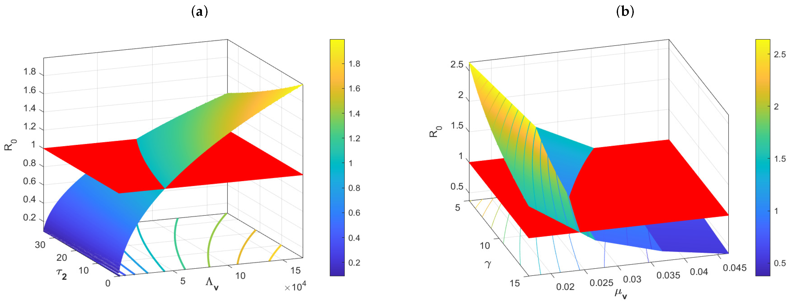
 Example 1. 

The impacts of the main parameters on the basic reproduction number ${\mathcal{R}}_0$.

The plots in Figure 2a imply that the incubation period ${\tau }_2$ of the pathogen in the vectors has an inhibitory effect on the spread of the disease, and that ignoring this delay overestimates ${\mathcal{R}}_0$ of the disease; whereas ${\mathcal{R}}_0$ is positively correlated with the recruitment rate ${\mathrm{\Lambda }}_v$ of the vector. In addition, Figure 2b also shows that ${\mathcal{R}}_0$ is negatively correlated with the death rate of hosts ${\mu }_v$ and the recovery rate $\gamma$ of hosts. This also implies that we can make ${\mathcal{R}}_0$ less than 1 by decreasing ${\mathrm{\Lambda }}_v$, increasing ${\mu }_v$ and $\gamma$. These numerical simulations overlap exactly with the expression for ${\mathcal{R}}_0$.

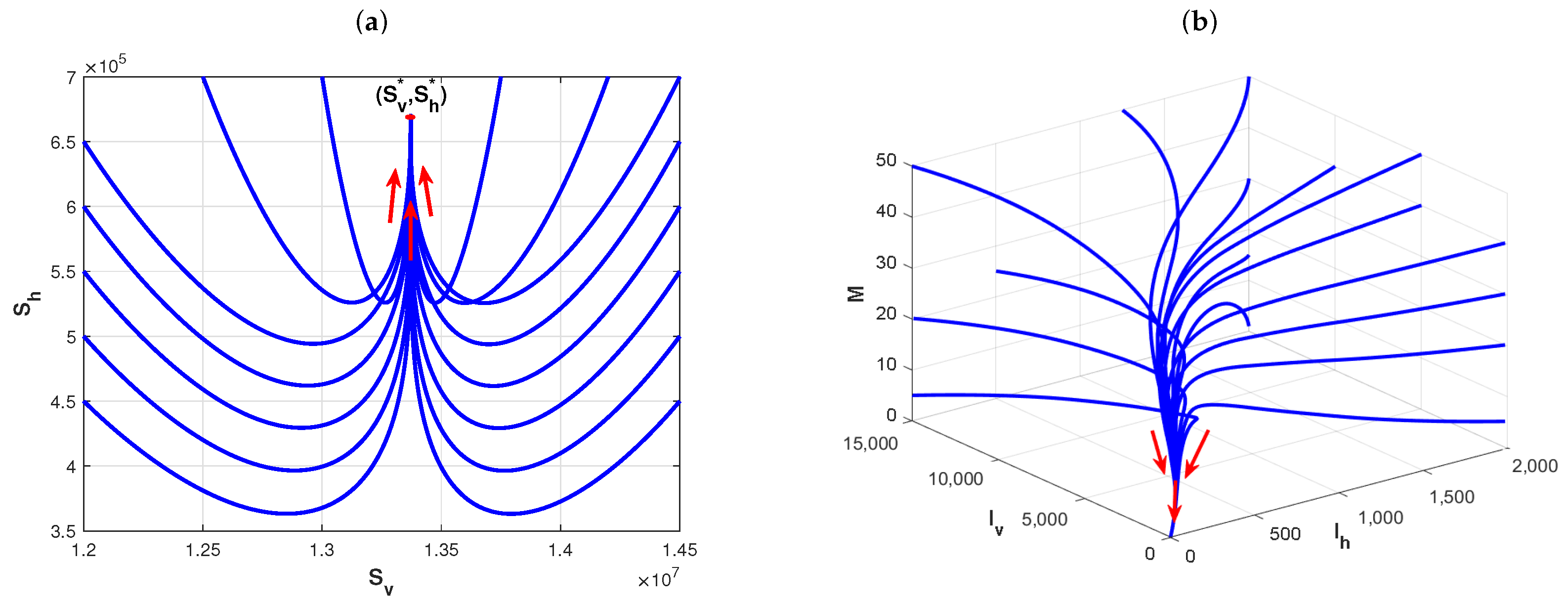
 Example 2. 

The existence and stability of disease-free and endemic equilibria of Model (1).

According to [7,14,19,20], the basic model parameters are fixed as follows: ${\mathrm{\Lambda }}_h=25.80$, ${\mu }_h=1/(71\times 365)$, ${\lambda }_v=6.686\times {10}^5$, $\eta =1/180$, $\gamma =1/10$. If we choose that ${\beta }_{vh}=1.75\times {10}^{-8}$, ${\beta }_{hv}=3.75\times {10}^{-8}$, ${\mu }_v=1/20$, $\kappa =0.001$, $\delta =0.0005$, ${\mu }_m=0.006$, ${\tau }_1=5$, and ${\tau }_2=10$. By direct calculation, the basic reproduction number is ${\mathcal{R}}_0\approx 0.8436<1$ in this case. 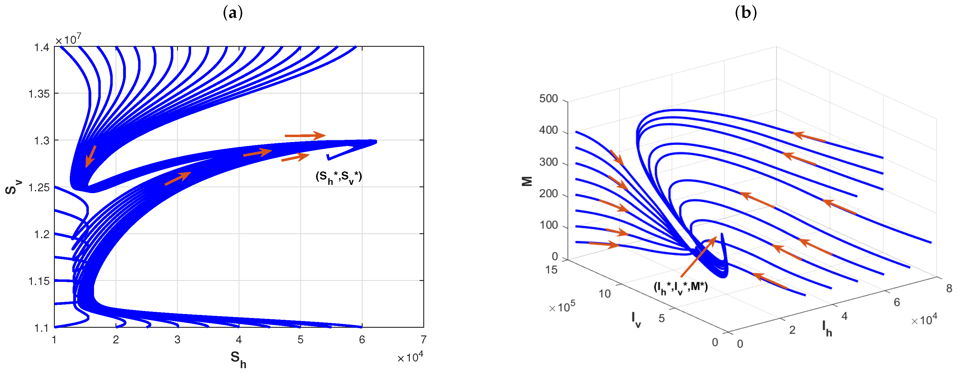Therefore, from Theorem 2, the disease-free equilibrium ${\mathcal{E}}_0=({\mathrm{\Lambda }}_h/{\mu }_h,0,0,0,{\mathrm{\Lambda }}_v/{\mu }_v,0)$ is asymptotically stable, which is shown in Figure 3a,b. This implies that the disease is ultimately eliminated. However, we’re just changing the values of ${\beta }_{hv}$ and ${\beta }_{vh}$ as ${\beta }_{vh}=6.75\times {10}^{-8}$ and ${\beta }_{hv}=1.75\times {10}^{-7}$, respectively, and other parameters are fixed as in Figure 3. By direct calculation, one has ${\mathcal{R}}_0\approx 3.5786>1$ in this case. The plots in Figure 4a,b show that the endemic equilibrium ${\mathcal{E}}^{*}=(S_h^{*},I_h^{*},R_h^{*},P_h^{*},S_v^{*},I_v^{*})$ of Model (1) is asymptotically stable.

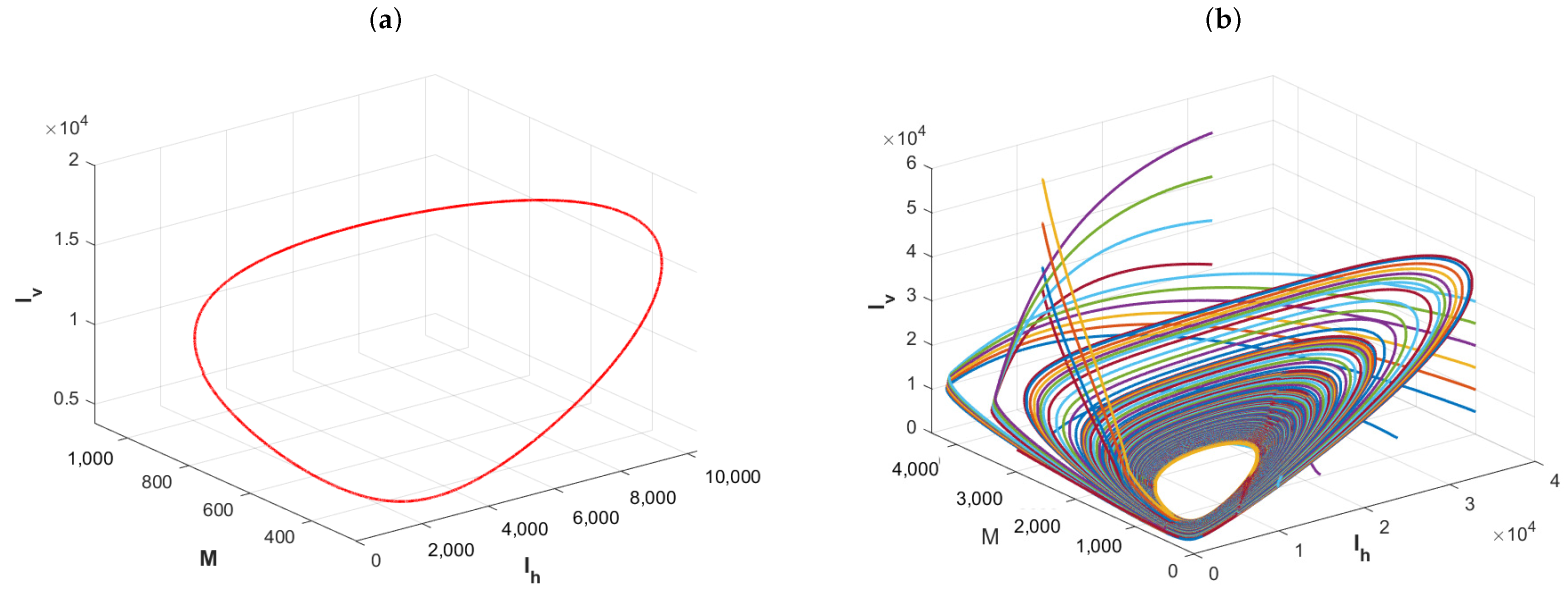
 Example 3. 

The effects of the delay for the distribution of infectious disease.

We fix the basic parameters of the model as follows: ${\mathrm{\Lambda }}_h=5.7882$, ${\mu }_h=1/(71\times 365)$, ${\mathrm{\Lambda }}_v=2.70\times {10}^4$ and ${\mu }_v=0.06$, which determine the sizes of the hosts and vector population. We choose, firstly, ${\beta }_{vh}={\beta }_{hv}=3.75\times {10}^{-6}$, $\alpha =0.4$, $\kappa =0.008$, $\eta =0.3$, $\gamma =0.09$, $\delta =0.006$, ${\mu }_m=0.05$, ${\tau }_1=45$ and ${\tau }_2=0$. In this case, ${\mathcal{R}}_0\approx 3.4363$ by the expression of the basic reproduction number. The plot in Figure 5a shows that Model (1) has a periodic solution, which is verified to be asymptotically stable by the plots of Figure 5b. Although it yields from the expression for the basic reproduction number ${\mathcal{R}}_0$ that delay ${\tau }_1$ is independent of ${\mathcal{R}}_0$, it can cause the disease to exhibit a cyclic oscillation phenomenon. Further, one changes, ${\beta }_{vh}=3.97\times {10}^{-7}$, ${\beta }_{hv}=3.91\times {10}^{-6}$, , $\alpha =0.02$, $\kappa =0.00038$, $\eta =0.12$, $\gamma =0.016$, $\delta =0.00015$, ${\mu }_m=0.08$, ${\tau }_1=0$, and ${\tau }_2=11$. By the direct calculation, it is clear that ${\mathcal{R}}_0\approx 7.5017>1$ in this case. The plot in Figure 6a shows that Model (1) admits a periodic solution and the plots in Figure 6b imply that the periodic solution is asymptotically stable. Numerical simulations imply that the delay ${\tau }_1$ in media coverage and the incubation period ${\tau }_2$ of pathogens in vectors are important factors, and ignoring them underestimates the complexity of vector-borne disease transmission.

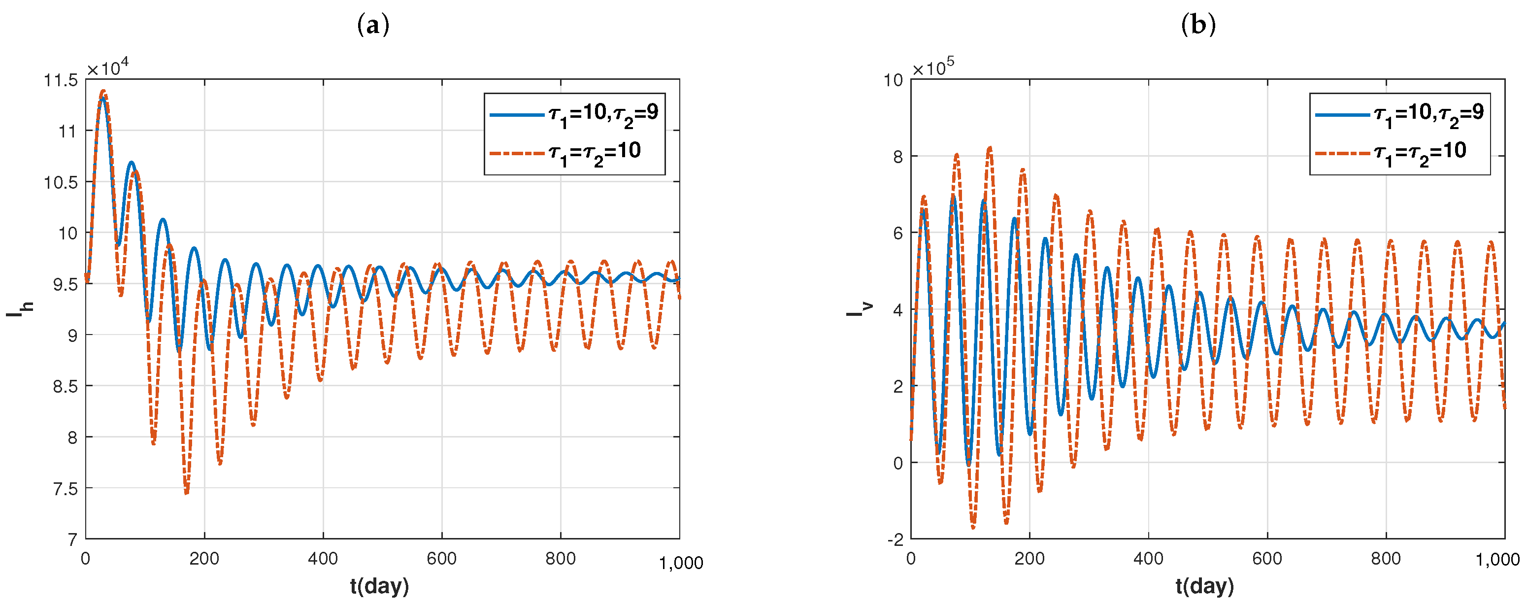
Now, we discuss the distribution of disease under the combined effects of the two delays ${\tau }_1$ and ${\tau }_2$. To this end, we choose two sets of delay parameters: $\left(i\right)$${\tau }_1=10$ and ${\tau }_2=9$; $\left(ii\right)$${\tau }_1={\tau }_2=10$, and other parameters are fixed as in Figure 6. By direct calculation, we find that the basic reproduction number ${\mathcal{R}}_0$ is approximately equal to 7.661706 in both cases. However, the trajectories of $I_h$ and $I_v$, that is, infected individuals, are shown by the blue solid lines and red dotted lines in Figure 7a,b, respectively. It is easy to see that the distributions of infected individuals have a very significant change under both sets of delay parameters. In other words, a small change in the delay will lead to a drastic fluctuation in the number of infected individuals. This is just like the old Chinese saying: every inch of the difference is a thousand miles away. Therefore, it is unreasonable to ignore the delay in the modeling of vector-borne diseases, and the accurate measurement of the incubation period of pathogens in vectors has an important impact on the prevention and control of diseases.

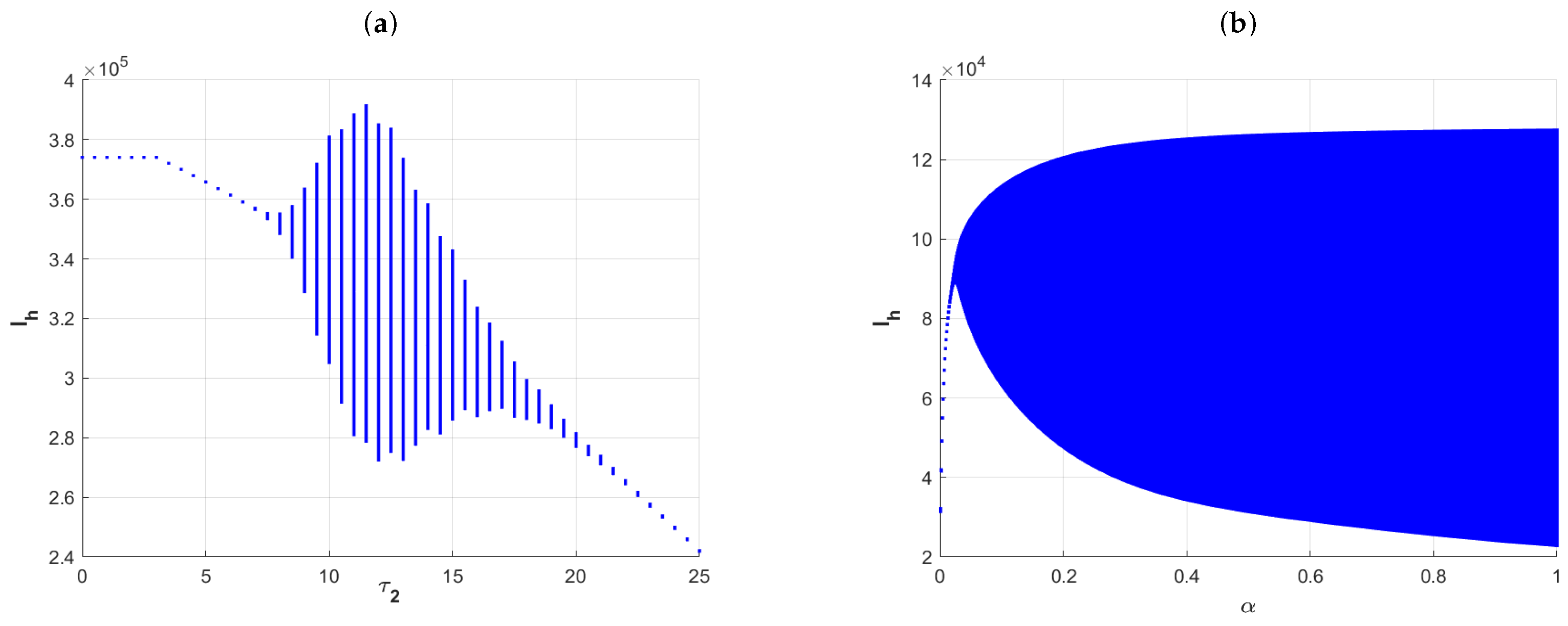
Finally, we consider the effects of the incubation delay of the pathogen $\left({\tau }_2\right)$ in the vectors and the duration of personal protection awareness (that is, $1/\alpha$, $\alpha$ is the rate of conscious susceptible transfers to unconscious susceptible)on the distribution of infected individuals. Here, the parameter ${\tau }_2$ is increased from 0 to 25, the parameter $\alpha$ is increased from 0 to 1, and the other parameters are fixed as in Figure 7. The plots in Figure 8a show that Model (1) has an endemic equilibrium while ${\tau }_2\in [0,7.25]$, whereas when ${\tau }_2\in (7.25,22.5)$, the number of infected individuals shows oscillations. This also implies that there is a periodic solution to the model in this case. And when ${\tau }_2\in (22.5,25)$, the model again has an endemic equilibrium. The plots in Figure 8b show the effect of $\alpha$ on the distribution of infected individuals, which implies that $\alpha$ has some significant effects on the size of the infected population. Specifically, the model has an endemic equilibrium state when a is very small, i.e., when the duration of personal protection awareness is maintained for a longer period of time, and the size of infected individuals is relatively low. And when $\alpha$ is relatively large, the model has a positive periodic solution, and the amplitude increases with $\alpha$. Numerical simulations show that rapid media response and a strong personal protection awareness can be effective in curbing the size of disease transmission.

7. Conclusions

As we all know, the incubation period of pathogens in vivo cannot be ignored in the spread of infectious diseases. It is directly related to the size and duration of disease outbreaks. In addition, the degree of harm of infectious diseases is also inextricably linked to the host’s race, living habits, behavioral habits, and knowledge structure. Thanks to the rapid development of the Internet, all kinds of media can more effectively provide people with information on public health and medical science, and disseminate to the public various policies and regulations on health prevention and disease control, so as to improve public health awareness, self-protection awareness and the ability to prevent and control infectious diseases, and curb the spread of diseases. Therefore, quantitatively portraying the incubation period of pathogens and the response speed of the media on disease transmission is one of the current hot issues in the prevention and control of infectious diseases. From the viewpoint of mathematical modeling, we propose a novelty model with multi-delays to discuss the effects of the above factors. In particular, our model also portrays the impact of news media on the personal behavior of susceptible individuals by introducing a compartment of susceptible individuals with personal protection (that is, $P_h$, perfect sense of personal protection, which can be found in [39,40,41]), and explores the role of the memory loss for presence awareness in disease prevention and control. This makes our model more consistent with the current characteristics of infectious disease transmission, which is one of the highlights of this article.

The exact expression of the basic reproduction number ${\mathcal{R}}_0$ is obtained, which can be used to determine the existence and stability of disease-free and endemic equilibria. Specifically, when the ${\mathcal{R}}_0$ is less than 1, the model exists only in the disease-free equilibrium, which is locally asymptotically stable, while when ${\mathcal{R}}_0$ is greater than 1, the model exists an unique endemic equilibrium in addition to the disease-free equilibrium. Additionally, we also obtain sufficient conditions for the local asymptotic stability of the endemic equilibrium. It should be especially emphasized here that, with delays as the bifurcation parameter, we also discussed the existence of the Hopf bifurcation, especially the direction and stability of the Hopf bifurcation applying the bifurcation theory. This is the other highlight of this paper.

Some numerical examples are carried out to explain the main theoretical results and investigate the sensitivity of the main parameters to the basic reproduction number. Our numerical simulations also show that the delay ${\tau }_1$ in media coverage has no effect on disease elimination and prevalence, which is consistent with our theoretical results. That is, the basic reproduction number is independent of ${\tau }_1$. But numerical simulations also show that ${\tau }_1$ affects the size of disease outbreaks (see Figure 5). In addition, numerical simulations also show that the sizes of the infected vectors and infected hosts fluctuate dramatically even when the basic reproduction number is almost equal under the combined effect of ${\tau }_1$ and ${\tau }_2$ (see Figure 7). This implies that ignoring or misestimating the magnitude of the delay can affect the accurate prevention and control of vector-borne diseases to varying degrees.

It should be noted that our initial intention is, in this paper, to portray the impact of a timely media response with perfect protection on the distribution of infectious diseases. In particular, in our model, we take into account the effect of forgetting mechanisms on the awareness of personal protection. Modeling vector-borne infections with imperfect protection and the effects of media delays is also an element of our future research. In addition, some factors are also ignored in the mathematical modeling process in order to perform the necessary theoretical analysis. For example, the effect of climate change and uncertainty on vector population size and behavior, the effect of vaccination on disease control, and the effect of spatial heterogeneity and frequent dispersal of host populations in space on the spatiotemporal distribution of disease, to name a few. These are also all worthy of further discussion.

References

1. World Health Organization. Weekly Epidemiological Update on COVID-19. Available online: https://www.who.int/publications/m/item/weekly-epidemiological-update-on-covid-19---19-january-2023 (accessed on 19 January 2023).
2. Ross, R. The Prevention of Malaria, 2nd ed.; Murray: London, UK, 1911. [Google Scholar]
3. MacDonald, G. The analysis of equilibrium in malaria. Trop. Dis. Bull. 1952, 49, 818–828. [Google Scholar]
4. Abdelrazec, A.; Lenhart, S.; Zhu, H. Transmission dynamics of West Nile virus in mosquitoes and corvids and non-corvids. J. Math. Biol. 2014, 68, 1553–1582. [Google Scholar] [CrossRef] [PubMed]
5. Garba, S.M.; Gumel, A.B.; Bakar, M.R.A. Backward bifurcations in dengue transmission dynamics. Math. Biosci. 2008, 215, 11–25. [Google Scholar] [CrossRef]
6. Simoy, M.I.; Aparicio, J.P. Vector-borne disease models with active and inactive vectors: A simple way to consider biting behavior. Bull. Math. Biol. 2022, 84, 22. [Google Scholar] [CrossRef]
7. Li, X.; Zou, X.; Cai, L.; Chen, Y. Global dynamics of a vector-borne disease model with direct transmission and differential susceptibility. J. Appl. Math. Comput. 2023, 69, 381–402. [Google Scholar] [CrossRef]
8. Rehman, A.; Ram, S.; Jagdev, S. Mathematical analysis of multi-compartmental malaria transmission model with reinfection. Chaos Soliton Fract. 2022, 163, 112527. [Google Scholar] [CrossRef]
9. Watts, H.; Mishra, A.; Nguyen, D.H. Dynamics of a vector-host model under switching environments. Discrete Cont. Dyn. B 2021, 26, 6463–6481. [Google Scholar] [CrossRef]
10. Jeffery, D.; Suzanne, L.; Sharon, B.; William, F. Implicit versus explicit vector management strategies in models for vector-borne disease epidemiology. J. Math. Biol. 2022, 84, 48. [Google Scholar]
11. Soufiane, B.; Salih, D.; Tarik, M.T.; Anwar, Z.; Abdon, A. Bifurcation analysis for a double age dependence epidemic model with two delays. Nonlinear Dynam. 2022, 108, 1821–1835. [Google Scholar]
12. Tarik, M.T.; Soufiane, B. Global analysis of an infection age model with a class of nonlinear incidence rates. J. Math. Anal. Appl. 2016, 434, 1211–1239. [Google Scholar] [CrossRef]
13. Abdelheq, M.; Salih, D.; Soufiane, B.; Kheireddine, B. Bifurcation analysis of a diffusive predator-prey model with prey social behavior and predator harvesting. Math. Methods Appl. Sci. 2022, 45, 718–731. [Google Scholar]
14. Wei, H.; Li, X.; Martcheva, M. An epidemic model of a vector-borne disease with direct transmission and time delay. J. Math. Anal. Appl. 2008, 342, 895–908. [Google Scholar] [CrossRef]
15. Bai, Z.; Zhou, Y. Global dynamics of an SEIRS epidemic model with periodic vaccination and seasonal contact rate. Nonlinear Anal.-Real. 2012, 13, 1060–1068. [Google Scholar] [CrossRef]
16. Zi, Z.; Kundu, S.; Tripathi, J.P.; Bugalia, S. Stability and Hopf bifurcation analysis of an SVEIR epidemic model with vaccination and multiple time delays. Chaos Soliton Fract. 2020, 131, 109483. [Google Scholar]
17. Xu, J.; Zhou, Y. Hopf bifurcation and its stability for a vector-borne disease model with delay and reinfection. Appl. Math. Model. 2016, 40, 1685–1702. [Google Scholar] [CrossRef]
18. Tanuja, D.; Prashant, K. Hopf bifurcation and stability switches in an infectious disease model with incubation delay, information, and saturated treatment. J. Appl. Math. Comput. 2022, 68, 4135–4159. [Google Scholar]
19. Cai, L.; Li, X.; Fang, B.; Run, S. Global properties of vector-host disease models with time delays. J. Math. Biol. 2017, 74, 1397–1423. [Google Scholar] [CrossRef]
20. Ding, C.; Tao, N.; Sun, Y.; Zhu, Y. The effect of time delays on transmission dynamics of schistosomiasis. Chaos Soliton Fract. 2016, 91, 360–371. [Google Scholar] [CrossRef]
21. Tian, D.; Song, H. Global dynamics of a Vector-Borne disease model with two delays and nonlinear transmission rate. Math. Methods Appl. Sci. 2017, 40, 6411–6423. [Google Scholar] [CrossRef]
22. Zhang, T.; Li, Z.; Ma, L.; Song, X. Threshold dynamics in a clonorchiasis model with time delays. Appl. Math. Model. 2022, 102, 351–370. [Google Scholar] [CrossRef]
23. Zhang, Y.; Huo, H.; Xiang, H. Dynamics of tuberculosis with fast and slow progression and media coverage. Math. Biosci. Eng. 2019, 16, 1150–1170. [Google Scholar] [CrossRef] [PubMed]
24. Shi, X.; Gao, X.; Zhou, X.; Li, Y. Analysis of an SQEIAR epidemic model with media coverage and asymptomatic infection. AIMS Math. 2021, 6, 12298–12320. [Google Scholar] [CrossRef]
25. Huo, H.; Yang, P.; Xiang, H. Stability and bifurcation for an SEIS epidemic model with the impact of media. Phys. A 2018, 490, 702–720. [Google Scholar] [CrossRef]
26. Liu, X.; Lv, Z.; Ding, Y. Mathematical modeling and stability analysis of the time-delayed SAIM model for COVID-19 vaccination and media coverage. Math. Biosci. Eng. 2022, 19, 6296–6316. [Google Scholar] [CrossRef]
27. Sharma, A.; Misra, A.K. Modeling the impact of awareness created by media campaigns on vaccination coverage in a variable population. J. Biol. Syst. 2014, 22, 249–270. [Google Scholar] [CrossRef]
28. Tchuenche, J.M.; Dube, N.; Bhunu, C.P.; Smith, R.J.; Bauch, C.T. The impact of media coverage on the transmission dynamics of human influenza. BMC Public Health 2011, 11, S5. [Google Scholar] [CrossRef]
29. Misra, A.K.; Sharma, A.; Singh, V. Effect of awareness programs in controlling the prevalence of an epidemic with time delay. J. Biol. Syst. 2011, 19, 389–402. [Google Scholar] [CrossRef]
30. Pawelek, K.A.; Oeldorf-Hirsch, A.; Rong, L. Modeling the impact of twitter on influenza epidemics. Math. Biosci. Eng. 2014, 11, 1337–1356. [Google Scholar] [CrossRef]
31. Song, P.; Xiao, Y. Analysis of an epidemic system with two response delays in media impact function. Bull. Math. Biol. 2019, 81, 1582–1612. [Google Scholar] [CrossRef]
32. Hu, L.; Nie, L. Dynamic modeling and analysis of COVID-19 in different transmission process and control strategies. Math. Methods Appl. Sci. 2021, 44, 1409–1422. [Google Scholar] [CrossRef]
33. Xue, L.; Ren, X.; Magpantay, F.; Sun, W.; Zhu, H. Optimal control of mitigation strategies for Dengue virus transmission. Bull. Math. Biol. 2021, 83, 8. [Google Scholar] [CrossRef] [PubMed]
34. Hale, J. Theory of Function Differential Equations; Springer: Heidelberg, Germany, 1977. [Google Scholar]
35. Astillo-Chávez, C.; Thieme, H.R. Asymptotically Autonomous Epidemic Models. In Mathematical Population Dynamics: Analysis of Heterogeneity, Vol. 1: Theory of Epidemics; Arino, O., Axelrod, D., Kimmel, M., Langlais, M., Eds.; Wuerz: Winnipeg, MB, Canada, 1995; pp. 33–50. [Google Scholar]
36. Busenberg, S.; Cooke, K.L. Vertically Transmitted Disease: Models and Dynamics; Springer: New York, NY, USA, 1993. [Google Scholar]
37. Freedman, H.I.; Sree Hari Rao, V. The trade-off between mutual interference and time lags in predator-prey systems. Bull. Math. Biol. 1983, 45, 991–1004. [Google Scholar] [CrossRef]
38. Hassard, B.D.; Kazariniff, N.D.; Wan, Y. Theory and Application of Hopf Bifurcation; London Mathematical Society Lecture Note Series; Cambridge University Press: London, UK, 1981; Volume 41. [Google Scholar]
39. Misra, A.K.; Shukla, J.B. Stability analysis and optimal control of an epidemic model with awareness programs by media. BioSystems 2015, 138, 53–62. [Google Scholar] [CrossRef] [PubMed]
40. Chukwu, C.W.; Nyabadza, F.; Fatmawati, F. Modelling the potential role of media campaigns on the control of Listeriosis. Math. Biosci. Eng. 2021, 18, 7580–7601. [Google Scholar] [CrossRef]
41. Rai, R.K.; Khajanchi, S.; Tiwari, P.K.; Venturino, E.; Misra, A.K. Impact of social media advertisements on the transmission dynamics of COVID-19 pandemic in India. J. Appl. Math. Comput. 2022, 68, 19–44. [Google Scholar] [CrossRef]
Figure 1. Flowchart of the transmission of pathogens between hosts and vectors.
Fractalfract 07 00831 g001
Figure 2. The impacts of the main parameters on the basic reproduction number R 0 : (a) The sensitivity of Λ v (the recruitment rate of vector) and τ 2 (the incubation delay of pathogen in the vectors) on R 0 ; (b) The sensitivity of μ v (the natural death rate of vectors) and γ (the recover rate of infected hosts) on R 0 .
Fractalfract 07 00831 g002
Figure 3. The asymptotic stability of the disease-free equilibrium E 0 of Model (1) with R 0 0.6360 : (a) The trajectories of ( S h , S v ) with differential initial values; (b) The trajectories of ( M , I h , I v ) with differential initial values.
Fractalfract 07 00831 g003
Figure 4. The asymptotic stability of the endemic equilibrium E * of Model (1) with R 0 3.5786 : (a) The trajectories of ( S h , S v ) with differential initial values; (b) The trajectories of ( I h , I v , M ) with differential values.
Fractalfract 07 00831 g004
Figure 5. The existence and stability of the periodic solution for model (1), where R 0 3.4363 , τ 1 = 45 , τ 2 = 0 : (a) The existence of periodic solution; (b) The stability of periodic solution.
Fractalfract 07 00831 g005
Figure 6. The existence and stability of the periodic solution for Model (1), where R 0 7.5017 , τ 1 = 0 , τ 2 = 11 : (a) The existence of periodic solution; (b) The stability of periodic solution.
Fractalfract 07 00831 g006
Figure 7. The combined effects of the two delays τ 1 and τ 2 on the distributions of infected individuals of Model (1), where the blue solid lines correspond to τ 1 = 10 and τ 2 = 9 ; the red dotted lines correspond to τ 1 = τ 2 = 10 : (a) The effects of τ 1 and τ 2 on the I h ; (b) The effects of τ 1 and τ 2 on the I v .
Fractalfract 07 00831 g007
Figure 8. The impacts of the main parameters on the distribution of infected hosts for model (1): (a) The effect of incubation delay τ 2 ; (b) The effect of rate of conscious susceptible transfers to unconscious susceptible α .
Fractalfract 07 00831 g008
Disclaimer/Publisher’s Note: The statements, opinions and data contained in all publications are solely those of the individual author(s) and contributor(s) and not of MDPI and/or the editor(s). MDPI and/or the editor(s) disclaim responsibility for any injury to people or property resulting from any ideas, methods, instructions or products referred to in the content.